Ab initio Full Cell GW+DMFT for Correlated Materials

Abstract

The quantitative prediction of electronic properties in correlated materials requires simulations without empirical truncations and parameters. We present a method to achieve this goal through a new ab initio formulation of dynamical mean-field theory (DMFT). Instead of using small impurities defined in a low-energy subspace, which require complicated downfolded interactions which are often approximated, we describe a full cell GW+DMFT approach, where the impurities comprise all atoms in a unit cell or supercell of the crystal. Our formulation results in large impurity problems, which we treat here with efficient quantum chemistry impurity solvers that work on the real-frequency axis, combined with a one-shot G₀W₀ treatment of long-range interactions. We apply our full cell approach to bulk Si, two antiferromagnetic correlated insulators NiO and $\alpha$-Fe₂O₃, and the paramagnetic correlated metal SrMoO₃, with impurities containing up to 10 atoms and 124 orbitals. We find that spectral properties, magnetic moments, and two-particle spin correlation functions are obtained in good agreement with experiment. In addition, in the metal oxide insulators, the balanced treatment of correlations involving all orbitals in the cell leads to new insights into the orbital character around the insulating gap.

I Introduction

Computing the properties of correlated electron materials with quantitative accuracy remains a fundamental challenge in ab initio simulations Kent and Kotliar (2018). This is because strong electron interactions, for example in materials with open $d$ or $f$ shells, can lead to emergent phases such as high-temperature superconductivity, which cannot be described by the mean-field and low-order perturbation approximations commonly employed by ab initio methods.

Quantum embedding methods Georges and Kotliar (1992); Georges et al. (1996); Knizia and Chan (2012); Sun and Chan (2016) in principle provide a promising route to access the phase diagrams of correlated materials, because they simultaneously treat strong local electron interactions and the thermodynamic limit. Among the different variants of quantum embedding used for this purpose, the combination of dynamical mean-field theory (DMFT) (and its cluster extensions Kotliar et al. (2001); Hettler et al. (2000)) and density functional theory (DFT) Kohn and Sham (1965), known as DFT+DMFT, is very popular Held et al. (2006); Kotliar et al. (2006); Held (2007). In this combination, one views DFT as a low-level theory that accounts for band structure and the long-range interactions, while the high-level solution of the DMFT impurity problem, defined on a small set of correlated orbitals, introduces diagrams arising from the strong local interactions. Yet despite many successes, DFT+DMFT does not provide a truly parameter-free and quantitative ab initio theory of correlated materials, due to two closely related issues. First, the local Coulomb interaction in the DMFT impurity problem is typically treated as an adjustable Hubbard-like parameter Nilsson and Aryasetiawan (2018), or is else estimated within another approximation Aryasetiawan et al. (2004). Second, a double-counting correction Wang et al. (2012); Haule (2015) is required to remove the DFT contribution to the local interactions, but no consistently accurate double-counting correction is known Karolak et al. (2010). Beyond these two primary concerns arising from the local interactions, density functionals also do not always reliably account for the long-range interaction effects Perdew et al. (2017).

To obtain a truly quantitative, ab initio formulation of DMFT, one must work within a diagrammatically clean formalism. In this context, it is natural to replace DFT with the GW approximation Hedin (1965) as the low-level theory. The GW approximation (often employed in its one-shot form (G₀W₀)) Hybertsen and Louie (1986); Shishkin and Kresse (2006) has been shown to fix many of the problems with semilocal density functionals (such as the underestimation of band gaps of weakly-correlated semiconductors) and thus appears a practical way to include the most important low-order long-range interaction diagrams. The combination with DMFT can then be formulated without double-counting by exactly subtracting the local GW contributions. The idea of self-consistently embedding the impurity self-energy and contributions to the polarization propagator arising from long-range interactions was proposed almost 18 years ago as the GW+(E)DMFT approximation Sun and Kotliar (2002); Biermann et al. (2003), but only very recently have self-consistent implementations appeared Boehnke et al. (2016); Nilsson et al. (2017). However, while these developments are promising, applications have remained more limited than those with DFT+DMFT and have retained some problematic issues of that approach Tomczak et al. (2012); Taranto et al. (2013); Tomczak et al. (2017); Choi et al. (2016, 2019); Petocchi et al. (2020). In particular, all current GW+(E)DMFT methods still require strongly downfolded interactions, because the impurity is restricted to the truncated low-energy subspace of a few correlated $d$ or $f$ orbitals (Fig. 1(b)). Downfolding to a small number of strongly coupled orbitals is numerically challenging, and yields retarded interactions that either limit the applicable impurity solvers or which must be truncated or otherwise approximated. If one ignores the embedding of the polarization propagator to work purely with the bare interactions, one obtains the self-energy embedding theory (SEET) Lan et al. (2017). However, applications of this simpler approach in realistic solids have only appeared very recently Iskakov et al. (2020). Aside from these technical issues, in some more complex correlated materials, the local orbitals can be intertwined with other itinerant bands Lu et al. (2008); Weber et al. (2010). In such cases, even defining a set of local correlated orbitals can be difficult, and the quality of the calculation then depends sensitively on this choice Amadon et al. (2008).

A common origin of many of the above challenges is the definition of the impurity problem in terms of a small low-energy subspace. This is done only to obtain as simple an impurity problem as possible, as motivated by model Hamiltonians, but it is not a requirement of the more general DMFT formalism. Consequently, in this work, we present a new formulation, which we term ab initio full cell GW+DMFT. In this approach we define the impurity to be the full unit cell - or even multiple unit cells of atoms - where each atom is described by a large localized set of atomic orbitals, covering the core, valence and high-energy virtual orbitals (Fig. 1(a)). Since no low-energy subspace is identified, there is no downfolding and its associated uncertainties, and we can simply use the full set of bare Coulomb interactions between the impurity orbitals, avoiding theoretical and numerical ambiguities. (A related full cell idea has been used to enable GW-in-DFT Green’s function embedding Chibani et al. (2016)). In addition, important medium range (non-local) interaction effects, weaker than the strongest local correlations, but stronger than the interactions captured by GW, can now enter the theory. (Such interactions, which are neglected in standard GW+DMFT treatments, are known to yield significant errors in a variety of settings, for example in the treatment of metallic sodium Nilsson et al. (2017)). While conceptually simple, our full cell approach engenders two new technical complexities. The first is the need to set up the large impurity problem (for example to efficiently generate all the matrix elements) but this is enabled by technical advances we have made in the PySCF simulation platform Sun et al. (2018) and our recently developed general ab initio quantum embedding framework Cui et al. (2020); Zhu et al. (2020). The second is the need to solve the resulting impurity problem with a large number of orbitals. Here, the key insight is that many orbitals in the full cell impurity are only weakly correlated, and impurity solvers which take advantage of this, such as those used in molecular quantum chemistry Zgid and Chan (2011); Zgid et al. (2012) can then work very efficiently. In this work, we will use two such kinds of solvers: a coupled-cluster singles and doubles (CCSD) Green’s function solver Zhu et al. (2019); Shee and Zgid (2019) as well as a selected configuration interaction (selected CI) solver Holmes et al. (2016), carrying out self-consistency along the real-frequency axis. The accuracy of such solvers in impurity problems has been benchmarked elsewhere Zgid et al. (2012); Lu et al. (2014); Go and Millis (2017); Zhu et al. (2019): thus we emphasize that a specific choice of the solver is not the message of this work. Rather, our focus is on establishing a generic full cell embedding framework that avoids downfolding and introduces new non-local physics at two levels of approximation at medium and large distances, and whose mathematical formulation allows a natural combination with a wide variety of quantum chemistry impurity solvers, including the two used here. We apply the full cell GW+DMFT method to compute the spectral properties of Si, the spectra, magnetic moments and spin correlation functions of two correlated insulators, NiO and $\alpha$-Fe₂O₃, in their antiferromagnetic (AFM) phases, as well as the spectra of a paramagnetic correlated metal SrMoO₃. Our largest calculation in hematite uses an impurity of four Fe and six O atoms, giving rise to an unprecedentedly large ab initio DMFT impurity problem with 124 impurity orbitals.

II Theory and implementation

In the full cell GW+DMFT formulation, because the impurity cell contains all atoms in a crystal cell (or, more usually, a supercell), the effects of what would normally be thought of as long-range interactions on the polarization and self-energy from within the supercell are all included. Also, because the supercell is treated at a level beyond GW, we include the medium-range interactions that are neglected in standard GW+DMFT treatments. However, we will treat contributions from long-range interactions beyond the supercell only at the level of the self-energy matrix of the crystal, computed at the one-shot G₀W₀ level. Because of this, certain contributions to the polarization propagator involving interactions far from the supercell, that would require the bosonic self-consistency of EDMFT Nilsson et al. (2017), are omitted. In practice, this means that rather than partitioning into the strictly strongest interactions (for example in a $d$- or $f$-shell), coupled to a low-level treatment of everything else as in standard GW+DMFT, our formulation prioritizes a higher-level treatment of interactions within a significant distance of the most correlated orbitals. The magnitude of the neglected effects from the lack of bosonic self-consistency, while ameliorated by the explicit treatment of large cells, can only be established through numerical experiments, as performed below. (An example of a case where the lack of bosonic self-consistency could be qualitatively important is in systems where there is an overlap of plasmon satellites and Hubbard bands Boehnke et al. (2016)).

Given a periodic crystal, we start by performing a one-shot G₀W₀ calculation on top of a mean-field reference (DFT or HF), using crystalline Gaussian atomic orbitals and Gaussian density fitting (GDF) integrals Sun et al. (2017). Because the G₀W₀ approximation is reference dependent, we will denote the approximation G₀W₀@reference. The full G₀W₀ self-energy matrix is computed in the mean-field molecular orbital (MO) basis along the imaginary-frequency axis Ren et al. (2012); Wilhelm et al. (2016):

$$\begin{split}{\mathbf{\Sigma}}_{nn^{\prime}}^{{\textit{GW}}}({\mathbf{k}},i\omega)=&-\frac{1}{2\pi}\sum_{m{\mathbf{k}}_{m}}\int_{-\infty}^{\infty}d\omega^{\prime}[{\mathbf{G}}_{0}({\mathbf{k}}_{m},i\omega-i\omega^{\prime})]_{mm}\\ &\times\sum_{PQ{\mathbf{k}}_{P}}v_{P}^{nm}[{\mathbf{I}}-{\mathbf{\Pi}}({\mathbf{k}}_{P},i\omega^{\prime})]_{PQ}^{-1}v_{Q}^{mn^{\prime}},\end{split}$$ (1)

where $v_{P}^{nm}$ represents the 3-index electron repulsion integral (ERI) ${\left(P{\mathbf{k}}_{P}\middle|n{\mathbf{k}}_{n}m{\mathbf{k}}_{m}\right)}$, $P$ is the Gaussian auxiliary basis, and $n$ and $m$ represent mean-field molecular orbitals (bands). ${\mathbf{k}}_{P}$, ${\mathbf{k}}_{n}$ and ${\mathbf{k}}_{m}$ satisfy crystal momentum conservation: ${\mathbf{k}}_{P}={\mathbf{k}}_{n}-{\mathbf{k}}_{m}+n\mathbf{b}$, where $\mathbf{b}$ is a lattice vector, and ${\mathbf{G}}_{0}({\mathbf{k}}_{m},i\omega-i\omega^{\prime})$ is the mean-field Green’s function. The integration in Eq. 1 is carried out efficiently using a modified Gauss-Legendre grid Ren et al. (2012) (100 grid points were used in this study). The polarization kernel ${\mathbf{\Pi}}({\mathbf{k}}_{P},i\omega^{\prime})$ is

$$\begin{split}{\mathbf{\Pi}}_{PQ}({\mathbf{k}}_{P},i\omega^{\prime})=2\sum_{i{\mathbf{k}}_{i}}^{{\mathrm{occ}}}\sum_{a{\mathbf{k}}_{a}}^{{\mathrm{vir}}}v_{P}^{ia}\frac{\epsilon_{i{\mathbf{k}}_{i}}-\epsilon_{a{\mathbf{k}}_{a}}}{\omega^{\prime 2}+(\epsilon_{i{\mathbf{k}}_{i}}-\epsilon_{a{\mathbf{k}}_{a}})^{2}}v_{Q}^{ai},\end{split}$$ (2)

where $\epsilon_{i{\mathbf{k}}_{i}}$ and $\epsilon_{a{\mathbf{k}}_{a}}$ are occupied and virtual orbital energies respectively. Note that in a Gaussian basis formulation, the number of bands and size of auxiliary basis are significantly smaller than in plane-wave GW formulations Booth et al. (2016), and because of this, the summations in Eqs. 1-2 run over all bands. To obtain the real-frequency G₀W₀ self-energy, we perform analytic continuation. Here, we fit the self-energy matrix elements to $N$-point Padé approximants ($N=18$ in this work) using Thiele’s reciprocal difference method Vidberg and Serene (1977). For the detailed G₀W₀ algorithm, we refer readers to Ref. Zhu and Chan (2020). Our G₀W₀ scheme thus allows us to use continuation to obtain the retarded self-energy on the real axis at arbitrary broadenings, although as an alternative, a contour deformation scheme Godby et al. (1988) may also be used to directly compute the real-frequency time-ordered self-energy without the need for analytic continuation. This latter strategy may be attractive to explore in the future to completely avoid possibly unstable analytic continuations.

To define the impurity problem, we first construct an orthogonal atom-centered local orbital (LO) basis. As in our previous work on ab initio HF+DMFT and density matrix embedding theory (DMET), we employ crystalline intrinsic atomic orbitals (IAOs) and projected atomic orbitals (PAOs) as the local orthogonal basis Knizia (2013); Cui et al. (2020); Zhu et al. (2020). IAOs are a set of valence atomic-like orbitals that exactly span the occupied space of the mean-field calculations, whose construction only requires projecting the DFT/HF orbitals onto predefined valence (minimal) AOs. PAOs, on the other hand, provide the remaining high-energy virtual atomic-like orbitals that complete the atomic basis and capture the correlation and screening effects.

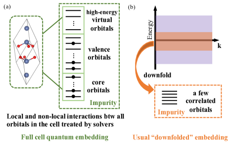
Figure 1: Illustration of (a) ab initio full cell GW+DMFT and (b) usual GW+DMFT schemes. In full cell embedding, all orbitals in the full unit cell (four Fe and six O atoms) are taken as the impurity in the $\alpha$-Fe₂O₃ calculation. In contrast, other GW+DMFT formulations define the impurity problem to contain a few correlated orbitals within a low-energy subspace which interact via downfolded, retarded, interactions.

The impurity consists of all LOs (i.e. all IAOs and PAOs) within the impurity cell (crystal cell or supercell) with IAOs representing the core and valence orbitals and PAOs representing the high-energy virtual orbitals. This is illustrated in Fig. 1(a). The most expensive step in forming the impurity Hamiltonian is computing the bare Coulomb interaction matrix ${\left(ij\middle|kl\right)}$ for all orbitals within the impurity cell. However, using Gaussian density fitting, we can do this at relatively low cost (scaling asymptotically as $\mathcal{O}(N_{{\mathbf{k}}}^{2}N_{L}N_{{\rm AO}}^{3})$, where $N_{{\mathbf{k}}}$, $N_{L}$ and $N_{{\rm AO}}$ are the numbers of ${\mathbf{k}}$ points and auxiliary Gaussian and atomic orbitals within the impurity cell). We refer readers to Ref. Zhu et al. (2020) for a detailed algorithm. The impurity Hamiltonian (without bath orbitals) is therefore

$$\hat{H}_{\mathrm{imp}}=\sum_{ij\in\mathrm{imp}}{\tilde{F}}_{ij}{a}^{\dagger}_{i}{a}_{j}\\ +\frac{1}{2}\sum_{ijkl\in\mathrm{imp}}{\left(ij\middle|kl\right)}{a}^{\dagger}_{i}{a}^{\dagger}_{k}{a}_{l}{a}_{j},$$ (3)

with the one-particle interaction $\tilde{F}_{ij}$ defined as the Hartree-Fock effective Hamiltonian with the double-counting term subtracted

$$\tilde{F}_{ij}=(F_{\mathrm{imp}})_{ij}-\sum_{kl\in\mathrm{imp}}(\gamma_{\mathrm{imp}})_{kl}[{\left(ij\middle|lk\right)}-\frac{1}{2}{\left(ik\middle|lj\right)}],$$ (4)

and with $\gamma_{\mathrm{imp}}$ as the impurity block of the mean-field density matrix.

We then start the DMFT cycle with an initial guess of the impurity self-energy as the G₀W₀ local self-energy: ${\mathbf{\Sigma}}_{\mathrm{imp}}(\omega)={\mathbf{\Sigma}}_{{\rm DC}}^{\textit{GW}}(\omega)$. The G₀W₀ local self-energy is computed in the LO basis within the impurity cell:

$$\begin{split}[{\mathbf{\Sigma}}_{{\rm DC}}^{{\textit{GW}}}(i\omega)]_{ij}=&-\frac{1}{2\pi}\sum_{kl}\int_{-\infty}^{\infty}d\omega^{\prime}[{\mathbf{G}}_{0}^{\mathrm{imp}}(i\omega-i\omega^{\prime})]_{kl}\\ &\times\sum_{RS}L_{R}^{ik}[{\mathbf{I}}-{\mathbf{\Pi}}(i\omega^{\prime})]_{RS}^{-1}L_{S}^{lj},\end{split}$$ (5)

and analytically continued to the real axis. Here, all local orbital indices ($i,j,k,l$) are within the impurity cell. The 3-index tensor $L_{R}^{ij}$ is computed from a Cholesky decomposition of the impurity ERI: ${\left(ij\middle|kl\right)}=\sum_{R}L_{R}^{ij}L_{R}^{kl}$. Note that the polarization propagator is computed in the impurity orbital space, first in the imaginary time domain Liu et al. (2016); Wilhelm et al. (2018):

$${\mathbf{\Pi}}_{RS}(\tau)=\sum_{ijkl\in\mathrm{imp}}L_{P}^{ij}[{\mathbf{G}}_{0}^{\mathrm{imp}}(\tau)]_{ki}L_{Q}^{kl}[{\mathbf{G}}_{0}^{\mathrm{imp}}(-\tau)]_{lj},$$ (6)

and then cosine transformed into imaginary frequency space.

The hybridization self-energy is then computed:

$${\mathbf{\Delta}}(\omega)=(\omega+\mu){\mathbf{I}}-\tilde{{\mathbf{F}}}-{\mathbf{\Sigma}}_{\mathrm{imp}}(\omega)-{\mathbf{G}}^{-1}(\mathbf{R}=\mathbf{0},\omega),$$ (7)

with the lattice Green’s function defined as

$${\mathbf{G}}(\mathbf{R}=\mathbf{0},\omega)=\frac{1}{N_{{\mathbf{k}}}}\sum_{{\mathbf{k}}}[(\omega+\mu){\mathbf{I}}-{\mathbf{h}}({\mathbf{k}})-{\mathbf{\Sigma}}({\mathbf{k}},\omega)]^{-1},$$ (8)

and the full GW+DMFT self-energy defined as

$${\mathbf{\Sigma}}({\mathbf{k}},\omega)={\mathbf{\Sigma}}^{\textit{GW}}({\mathbf{k}},\omega)+{\mathbf{\Sigma}}_{\mathrm{imp}}(\omega)-{\mathbf{\Sigma}}_{\rm DC}^{\textit{GW}}(\omega).$$ (9)

Here, $\mu$ is the chemical potential, which is adjusted during the DMFT self-consistency to ensure that the electron count of the impurity is correct. ${\mathbf{h}}({\mathbf{k}})$ is the bare one-particle Hamiltonian for the whole solid. We subtract the local G₀W₀ self-energy in Eq. 9, and the DFT exchange-correlation potential is excluded from both the impurity and lattice self-energies, consequently our method exactly avoids double-counting. When the one-shot G₀W₀ is used, it is not guaranteed that the GW+DMFT self-energy in Eq. 9 is strictly causal, and a fully self-consistent GW+DMFT is formally required Lee and Haule (2017). However, in our test cases, we have not observed non-causal negative spectral functions at low-energies. Because multiple orbitals and atoms are now chosen as the impurity, the final GW+DMFT self-energy does not strictly preserve all the symmetries of the solid, similar to other cellular DMFT methods Kotliar et al. (2001). Possible ways to alleviate this problem include incorporating more cells as the impurity, or deriving a translational and crystal symmetry invariant impurity Hamiltonian, as done in the dynamical cluster approximation (DCA) Hettler et al. (2000).

In order to use a wavefunction (Hamiltonian-)based impurity solver, we discretize ${\mathbf{\Delta}}(\omega)$. We discretize along the real-frequency axis de Vega et al. (2015) so that dynamical quantities (e.g., spectral functions) are obtained more accurately. To obtain the discretization, we start with an initial guess by direct discretization on a numerical grid and optimize bath couplings $\{V_{ip}^{(n)}\}$ and energies $\{\epsilon_{n}\}$ to minimize a cost function over a range of real-frequency points (see Supplemental Material):

$$D=\sum_{\omega_{l}}\sum_{ij}\Big{(}\Delta_{ij}(\omega_{l}+i\eta)-\sum_{n=1}^{N_{\epsilon}}\sum_{p=1}^{N_{p}}\frac{V_{ip}^{(n)}V_{jp}^{(n)}}{\omega_{l}+i\eta-\epsilon_{n}}\Big{)}^{2},$$ (10)

where $N_{\epsilon}$ is the number of bath energies and $N_{p}$ is the number of bath orbitals per bath energy, and we use a broadening factor $\eta=0.1$ a.u. unless specified. This optimization scheme is necessary to reduce the number of bath orbitals and avoid non-causal behavior in the GW+DMFT self-energies. The bath degrees of freedom are truncated by only coupling bath orbitals to the valence IAOs, further reducing computational and optimization costs. The full embedding problem with both impurity and bath orbitals is thus defined from the Hamiltonian

$$\hat{H}_{\mathrm{emb}}=\hat{H}_{\mathrm{imp}}+\sum_{n=1}^{N_{\epsilon}}\sum_{p=1}^{N_{p}}\Big{(}\sum_{i}V_{ip}^{(n)}(a_{i}^{\dagger}a_{np}+a_{np}^{\dagger}a_{i})+\epsilon_{n}a_{np}^{\dagger}a_{np}\Big{)}.$$ (11)

We solve for the ground-state and Green’s functions of the impurity Hamiltonian using two quantum chemistry impurity solvers. For completeness, we give some general background on the solvers. The first is a CCSD Green’s function solver at zero temperature. Our implementation of the CCSD Green’s function solver is able to treat around 200 (impurity + bath) orbitals. At the singles and doubles level, CC may be viewed as generating ring, ladder, and coupled ring-ladder diagrams, and is exact for (arbitrary products of) two-electron problems regardless of interaction strength. CCSD is based on time-ordered diagrams, and the corresponding CCSD Green’s function does not include contributions from all time-orderings of the ring diagrams that come from the GW self-energy, but contains a large number of vertex corrections to the self-energy and polarization propogator Lange and Berkelbach (2018). It has been shown to be accurate in a variety of settings, including simple metallic and ordered magnetic states in ab initio calculations McClain et al. (2016); Gao et al. (2020); Williams et al. (2020), across weak to strong couplings when employed with small cluster DMFT impurities in Hubbard-like models Zhu et al. (2019), and in electron gases up to moderately dilute densities, e.g. that of metallic sodium McClain et al. (2016). Standard implementations of CCSD are capable of treating general Coulomb interactions and hybridizations, and recent work has demonstrated ab initio calculations in materials at finite temperatures White and Chan (2018); White and Kin-Lic Chan (2020). Similar to other quantum chemistry based approaches, the efficiency of the CCSD method stems from taking advantage of the fact that many orbitals (e.g., far from the Fermi surface) are nearly full or empty. However, it is less suited to spin-fluctuations, and because CCSD truncates the coupled-cluster excitations at low order, it will break down when large spin fluctuations connecting many electrons simultaneously appear. In practice, a key indicator for the breakdown of CCSD is the magnitude of its excitation amplitudes, with large amplitudes suggesting inaccurate results.

In cases where CCSD breaks down, one can use higher excitation levels in CC McClain et al. (2016), or other impurity solvers can be employed. Other interesting quantum chemistry solvers in this context include quantum chemistry DMRG (QC-DMRG) Chan and Sharma (2011) and selected configuration interaction (selected CI) Holmes et al. (2016); Huron et al. (1973); Mejuto-Zaera et al. (2019); Zgid et al. (2012) methods. For example, QC-DMRG offers a robust way to obtain correlated ground-states in complex systems Li et al. (2019) and ab initio Green’s functions with up to 50 or more strongly correlated orbitals Ronca et al. (2017). Selected CI methods are based on an excitation picture, and thus are very efficient with large numbers of nearly filled and empty orbitals ($\sim$200), although they are limited to smaller numbers of strongly correlated orbitals than DMRG ($\sim$20). These two solvers are systematically improvable towards numerical exactness, by decreasing the selection threshold (selected CI) or increasing the bond dimension (DMRG). To illustrate the generality of our embedding framework as well as to benchmark the accuracy of the CCSD solver, we show results also from a selected CI impurity solver (based on the semistochastic heat-bath configuration interaction (SHCI) method Holmes et al. (2016); Sharma et al. (2017); Li et al. (2018); Yao et al. ) within our GW+DMFT approach and apply it to the correlated metal SrMoO₃.

From the impurity Green’s functions computed by the CCSD or SHCI solvers, we obtain an updated impurity self-energy ${\mathbf{\Sigma}}_{\mathrm{imp}}(\omega)$, and from this the DMFT cycle (Eqs. 7-11) is iterated until convergence between the impurity and lattice Green’s functions:

$${\mathbf{G}}_{\mathrm{imp}}(\omega)={\mathbf{G}}(\mathbf{R}=\mathbf{0},\omega).$$ (12)

III Results

We first apply our method to crystalline silicon. Although Si is considered a weakly-correlated semiconductor, it is still a challenging system for many DFT functionals (such as LDA and GGA) which do not yield accurate band gaps Heyd et al. (2005). One-shot G₀W₀ on top of LDA or GGA is known to significantly improve the band structure, although this relies somewhat on the cancellation of errors Shishkin et al. (2007). Such a small band-gap system also poses challenges to quantum embedding methods that start from a local correlation picture, such as DMFT Zein et al. (2006), due to the long-range nature of its statically screened Coulomb interaction, which must be included in the treatment.

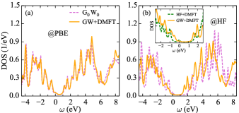
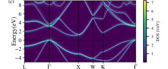
Figure 2: Full cell GW+DMFT results for silicon. (a)(b) Local spectral function from GW+DMFT (PBE reference) and GW+DMFT (HF reference). Inset of (b): GW+DMFT compared to HF+DMFT ($4\times 4\times 4$ ${\mathbf{k}}$-mesh and GTH-DZVP basis) DOS taken from Ref. Zhu et al. (2020). (c) Band structure starting from PBE orbitals. The heat map represents the GW+DMFT@PBE result and the dashed line gives the G₀W₀ bands. A broadening factor of 0.1 eV is used.

The full cell GW+DMFT results for Si are presented in Fig. 2. We used the GTH-PADE pseudopotential Hartwigsen et al. (1998) and GTH-TZVP basis Vandevondele et al. (2005), and a $6\times 6\times 6$ $\Gamma$-centered ${\mathbf{k}}$-point sampling. The impurity was defined as the unit cell of 2 Si atoms with 34 local orbitals ($3s3p3d4s4p5s5p$ for Si), and 128 bath orbitals were used. As known from other G₀W₀ calculations Fuchs et al. (2007) and as seen in Figs. 2(a) and 2(b), the mean-field starting point strongly affects the quality of the G₀W₀ results; G₀W₀@PBE gives an accurate band gap of 1.09 eV when compared to the experimental value of 1.17 eV O’Donnell and Chen (1991), while G₀W₀@HF overestimates the band gap, giving 2.04 eV. GW+DMFT predicts the band gap of Si to be 1.01 eV (@PBE) and 1.39 eV (@HF), largely removing the reference dependence of G₀W₀, due to the more complete inclusion of diagrams from interactions within the unit cell. The spectral function is also greatly improved in GW+DMFT compared to G₀W₀@HF. In earlier HF+DMFT calculations Zhu et al. (2020) (see inset of Fig. 2(b)), we found the band gap to be too large by 0.5 eV, and this quantifies the effect of the long-range correlations in G₀W₀ on the band gap of Si. From Fig. 2(c), we note that GW+DMFT@PBE maintains the accurate band structure of G₀W₀@PBE, in contrast to self-consistent GW, which is known to lead to worse results than G₀W₀ itself Shishkin and Kresse (2007); Kutepov (2017).

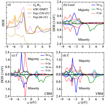
Figure 3: Full cell GW+DMFT results for NiO (AFM phase) based on the PBE reference. (a) Local DOS. The experimental spectra are taken from Ref. Sawatzky and Allen (1984). (b) Orbital-resolved local DOS. (c)(d) Orbital-resolved and momentum-resolved DOS at the $\Gamma$ point (CBM) and $\mathrm{Z}=(0.5,0.5,0.5)$ point (VBM). A broadening factor of 0.4 eV is used.

We next show the results of full cell GW+DMFT in Fig. 3 for a strongly-correlated insulator, NiO, in the antiferromagnetic phase. The GTH-PADE pseudopotential and GTH-DZVP-MOLOPT-SR basis set VandeVondele and Hutter (2007) were used with a $6\times 6\times 6$ $\Gamma$-centered ${\mathbf{k}}$-point sampling defined with respect to the antiferromagnetic cell (2 NiO units). (As an estimate of the remaining finite size error, the difference between the G₀W₀@PBE gaps for $4\times 4\times 4$ and $6\times 6\times 6$ ${\mathbf{k}}$-meshes is only 0.1 eV). We used the antiferromagnetic cell of 2 NiO units along the [111] direction as the impurity, corresponding to 78 impurity orbitals ($3s3p3d4s4p4d4f5s$ for Ni and $2s2p3s3p3d$ for O) and 72 bath orbitals in the DMFT impurity problem. As seen in Fig. 3(a), G₀W₀@PBE severely underestimates the band gap at 1.9 eV, even when using a spin symmetry broken PBE reference. We note that the quality of GW in this material is strongly dependent on the initial choice of Hamiltonian, and in practice improves through self-consistency, as has been seen in self-consistent quasiparticle GW calculations Kotani et al. (2007). Meanwhile, the valence spectrum of G₀W₀@PBE does not agree well with the experimental photoemission spectrum measured at a photon energy of 120 eV Sawatzky and Allen (1984). We note that the experimental spectra do not report photoemission intensity in absolute units, so we rescale the spectra to make the main valence peaks of the experimental and GW+DMFT spectra approximately the same height, to facilitate comparison. GW+DMFT, on the other hand, predicts a band gap of 4.0 eV and a magnetic moment of 1.69 $\mu_{B}$, both in very good agreement with the experimental values of 4.3 eV Sawatzky and Allen (1984) and 1.77-1.90 $\mu_{B}$ Fender et al. (1968); Cheetham and Hope (1983). More interestingly, our GW+DMFT DOS captures the experimental two-peak structure of the valence spectrum around $-2$ and $-3$ eV. A detailed analysis of the spin-orbital-resolved local DOS in Fig. 3(b) reveals that this two-peak structure results from the splitting of the majority and minority spin components of the Ni-$t_{2g}$ orbitals, and is a signature of the AFM phase, as it does not arise within the paramagnetic phase Kang and Choi (2019). Compared to the experimental valence spectrum measured at a lower photon energy (66 eV) that mainly probes O-$2p$ states, we find that our GW+DMFT DOS agrees very well with the experimental peak at -5 eV, suggesting we have achieved a quantitative description of both local and non-local states in NiO. Our GW+DMFT method also predicts a satellite peak around -8 eV, consistent with the photoemission spectrum in Ref. Van Elp et al. (1992). We find this valence peak has a significant contribution from O-$2p$ orbitals, and a less substantial Ni-$3d$ weight. From the local DOS, we can also conclude that NiO is an insulator with mixed charge-transfer and Mott character, with a valence band with contributions from Ni-$t_{2g}$, Ni-$e_{g}$ and O-$2p$, and a conduction band that is mainly of Ni-$e_{g}$ character.

In Figs. 3(c) and 3(d), we further analyze the character of the conduction band minimum (CBM) and valence band maximum (VBM) in the Brillouin zone using the momentum-resolved DOS. We find that the lowest conduction band has strong Ni-$4s$ and O-$2s$ character at the $\Gamma$ point (CBM), which was not discussed in many earlier DMFT calculations Kuneš et al. (2007); Leonov et al. (2016); Choi et al. (2016) which focused on the Ni-$3d$ and O-$2p$ orbitals and thus did not include Ni-$4s$ (or O-$2s$) orbitals in the impurity (although see Ref. Zhang et al. (2019) for a notable exception), unlike our full cell GW+DMFT treatment. At the Z point (VBM), we find that the highest valence band has significant O-$2p$ and Ni-$e_{g}$ contributions, with very little Ni-$t_{2g}$ character. This is very different from the local DOS, where the Ni-$t_{2g}$ has dominant weight in the valence bands. We confirm this by plotting the spatially-resolved DOS of NiO in the (001) plane in Fig. 4. We see that at the first valence peak and around the Ni atoms, the local spatial DOS has a Ni-$t_{2g}$ ($d_{xy}$) orbital shape, while the momentum-resolved spatial DOS (at the Z point) has a Ni-$e_{g}$ ($d_{x^{2}-y^{2}}$) orbital shape. Further, the weight of the DOS around the O atoms in Fig. 4(b) is considerably larger than in Fig. 4(a).

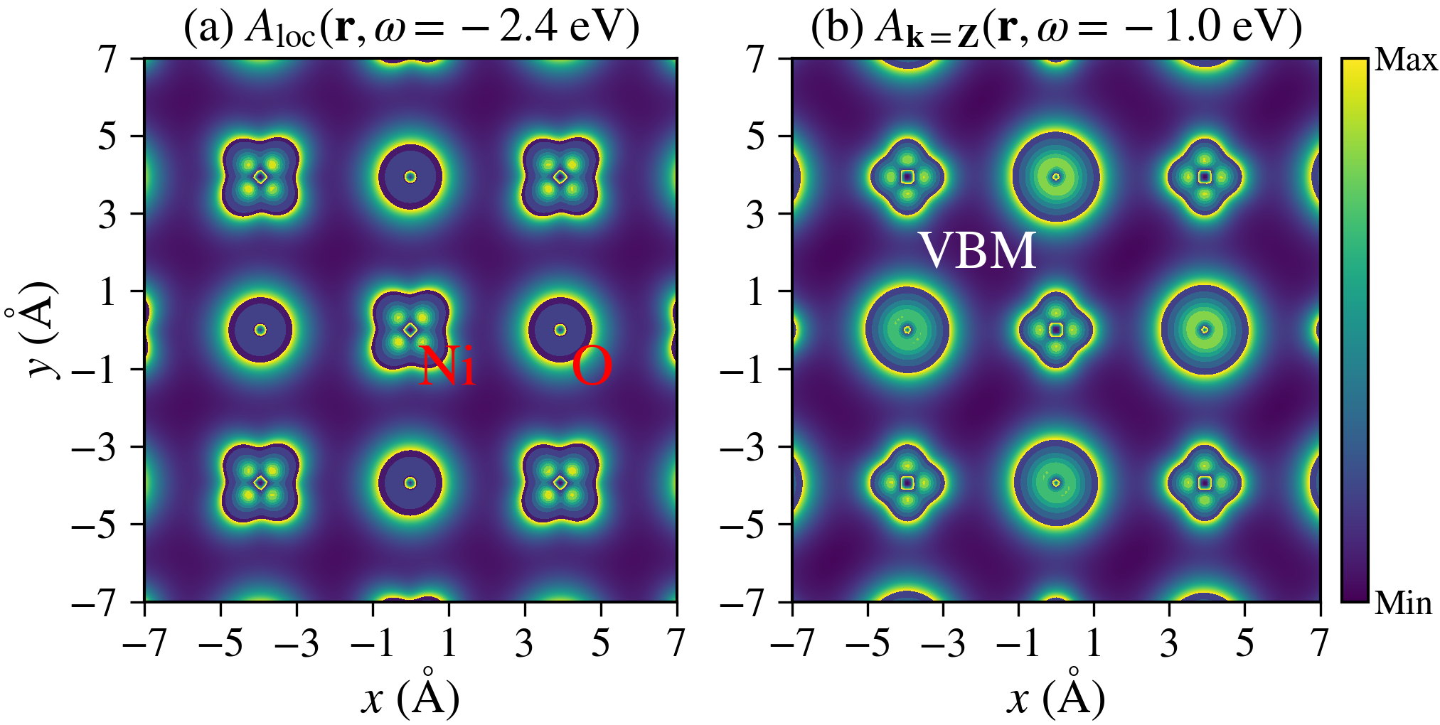
Figure 4: Spatially-resolved DOS from GW+DMFT (PBE reference) for NiO in the (001) plane. (a) Local DOS at $\omega=-2.4$ eV. (b) Momentum-resolved DOS at VBM energy $\omega=-1.0$ eV and $\mathrm{Z}=(0.5,0.5,0.5)$ point.

Since our impurity includes two NiO units, we can also look at correlations across the cells. We computed the spin-spin correlation function for the Ni atoms within the impurity problem:

$$\sum_{{i\in\mathrm{Ni}_{1},j\in\mathrm{Ni}_{2}}}\langle\mathbf{S}_{i}\cdot\mathbf{S}_{j}\rangle=\sum_{{i\in\mathrm{Ni}_{1},j\in\mathrm{Ni}_{2}}}\sum_{a=x,y,z}\langle S_{i}^{a}S_{j}^{a}\rangle.$$ (13)

We found $\langle\mathbf{S}_{i}\cdot\mathbf{S}_{j}\rangle$ between two Ni atoms to be -0.707. Both $\langle S_{i}^{x}S_{j}^{x}\rangle$ and $\langle S_{i}^{y}S_{j}^{y}\rangle$ contribute almost zero spin correlation, and the uncorrelated value $\langle S_{i}^{z}\rangle\langle S_{j}^{z}\rangle$ is -0.710, suggesting that quantum spin correlations are weak and NiO is close to a classical Ising magnet. This is consistent with experimental measurements of the critical behavior of the magnetic phase transition in NiO Chatterji et al. (2009) and our previous ab initio DMET study Cui et al. (2020).

We next turn to study a second strongly-correlated insulator, hematite ($\alpha$-Fe₂O₃), in the AFM phase. We take the impurity to be the complete AFM unit cell, including 2 Fe₂O₃ units (Fig. 1), with a “$+-+-$” type AFM ordering of the Fe spins. Because of the large impurity size, we used a DZV-quality basis (GTH-DZV-MOLOPT-SR, $3s3p3d4s4p4d5s$ for Fe, $2s2p3s3p$ for O), leading to an impurity problem with 124 impurity and 48 bath orbitals. The small number of bath orbitals is due to the current numerical limitations of our CCSD solver. However, since our bath orbitals are only coupled to the valence impurity orbitals, and we aim to reproduce the hybridization only in a window near the Fermi level ($\pm 0.4$ a.u.), the bath discretization error is not too severe. Numerical tests (Supplemental Material) suggest that the finite bath discretization introduces an error of 0.05 $\mu_{B}$ in the Fe magnetic moment, while the band gap uncertainty is within 0.4 eV. The $3s3p$ orbitals of Fe were treated as frozen core orbitals (i.e., uncorrelated) in the CCSD solver. The GTH-PBE pseudopotential and $4\times 4\times 4$ $\Gamma$-centered ${\mathbf{k}}$-point sampling were employed. As presented in Fig. 5(a), G₀W₀@PBE severely underestimates the band gap at 0.5 eV, compared to the experimental value of 2.6 eV Zimmermann et al. (1999). G₀W₀ with the hybrid functional PBE0 slightly overestimates the gap (3.4 eV), but the spectrum does not agree well with experiment, and in particular, the features of the G₀W₀@PBE0 DOS are too sharp around -7 and 3.5 eV (Fig. 5(b)).

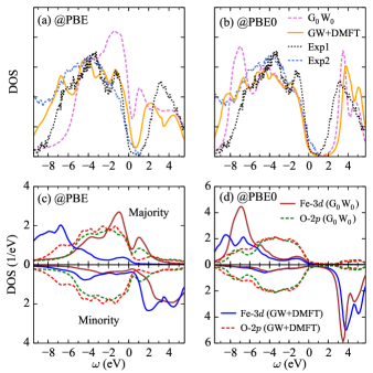
Figure 5: Full cell GW+DMFT results for $\alpha$-Fe₂O₃ (AFM phase). (a)(b) Local DOS based on PBE and PBE0 references. The experimental spectra are taken from Ref. Zimmermann et al. (1999) (exp1) and Ref. Fujimori et al. (1986) (exp2). (c)(d) Orbital-resolved DOS corresponding to (a)(b). A broadening factor of 0.3 eV is used.

GW+DMFT improves the G₀W₀@PBE spectrum significantly, especially in the valence region, although the band gap (1.5 eV) is still too small. From the orbital-resolved DOS in Fig. 5(c), we find that the main improvement comes from the spectral positions of the majority spin component of the Fe-$3d$ orbitals and O-$2p$ orbitals. G₀W₀@PBE mistakenly predicts the Fe-$3d$ valence spectrum to lie close to the Fermi level and that Fe₂O₃ has considerable Mott insulating character. However, GW+DMFT shifts the majority-spin Fe-$3d$ DOS to lower energies, consistent with previous DFT+DMFT calculations Kuneš et al. (2009); Greenberg et al. (2018). Because of this correction, GW+DMFT obtains a more accurate Fe magnetic moment than PBE (4.23 $\mu_{B}$ compared to 3.71 $\mu_{B}$ with the experimental moment being 4.64 $\mu_{B}$ Coey and Sawatzky (1971)). While the GW+DMFT DOS does not agree well with the “exp1” spectrum Zimmermann et al. (1999) below -7 eV, we observe a much better agreement between GW+DMFT and the “exp2” spectrum Fujimori et al. (1986), likely due to different experimental settings. We find that the valence band spectrum is dominated by O-$2p$ near the Fermi level, indicating that Fe₂O₃ is in fact a pure charge-transfer insulator, with almost no Mott insulating character. This is in contrast to DFT+DMFT calculations Kuneš et al. (2009); Greenberg et al. (2018) that find a sizable Fe-$3d$ contribution to the valence band maximum. We attribute this disagreement to the full cell GW+DMFT treatment where both O-$2p$ orbitals and Fe-$3d$ are treated on an equal footing at the impurity level, which thus allows for a more accurate balancing of their relative contributions to the spectral weight.

Starting from a PBE0 reference, GW+DMFT finds a slightly larger band gap (3.9 eV) and magnetic moment (4.37 $\mu_{B}$) than G₀W₀ (3.4 eV and 4.20 $\mu_{B}$). The overly sharp peaks of the G₀W₀@PBE0 spectrum around $-7$ and 3.5 eV are corrected by GW+DMFT, which broadens the Fe-$3d$ peaks as shown in Fig. 5(d). Comparing results between the PBE and PBE0 references, the severe reference dependence of spectral functions (especially Fe-$3d$ states) is largely reduced by GW+DMFT. In summary, it appears we achieve a good description of the photoemission spectrum for Fe₂O₃ within the full cell GW+DMFT, although a fully quantitative prediction of the band gap is not attained. Given that G₀W₀ only provides a minor correction to the underlying DFT band gap in this system, the likely culprit is the insufficiency of the G₀W₀ approximation in describing the long-range interactions in Fe₂O₃.

We finally investigate a perovskite-type paramagnetic correlated metal SrMoO₃ with two electrons ($4d^{2}$) occupying the Mo-$t_{2g}$ bands. We simulated the cubic structure of SrMoO₃ using the GTH-PADE pseudopotential and GTH-DZVP-MOLOPT-SR basis set, with a $\Gamma$-centered $6\times 6\times 6$ ${\mathbf{k}}$-mesh. To facilitate comparison with previous numerical studies, we used LDA as the underlying DFT functional. The SrMoO₃ unit cell was taken as the DMFT impurity, corresponding to 71 impurity orbitals ($4d4f5s5p5d6s$ for Mo, $2s2p3s3p3d$ for O, $4d5s5p6s$ for Sr) and 117 bath orbitals. For paramagnetic metals, the quasiparticle peaks are expected to be sharp near the Fermi level, so we used a much smaller broadening ($\eta=0.02$ a.u.) when discretizing the hybridization on the real axis. We found this small broadening is crucial for avoiding non-causal behavior in the computed self-energies.

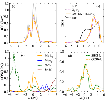
Figure 6: Full cell GW+DMFT results for paramagnetic SrMoO₃ based on the LDA reference. (a) Local DOS of Mo-$t_{2g}$ bands computed with a broadening of 0.15 eV. (b) Comparison of G₀W₀ and GW+DMFT with photoemission experimental data Wadati et al. (2014). A Fermi function of 298 K and a Gaussian filter of 0.2 eV are applied to the calculated DOS to match the experimental resolution. (c) Orbital-resolved DOS computed by GW+DMFT (CCSD). (d) Comparison of GW+DMFT DOS (Mo-$t_{2g}$ bands) using CCSD and SHCI solvers in a frozen-core correlated space.

As the electronic structure of SrMoO₃ near the Fermi level is dominated by Mo-$t_{2g}$ bands, we mainly discuss spectral functions of Mo-$t_{2g}$ bands in Fig. 6, although the orbital-resolved DOS is also included in Fig. 6(c). As shown in Fig. 6(a), G₀W₀@LDA shows a small band narrowing compared to LDA, where the bandwidth is reduced from 3.9 eV (LDA) to 3.2 eV (G₀W₀). GW+DMFT with the CCSD solver predicts a slightly larger bandwidth of 3.5 eV than G₀W₀ and similar quasiparticle bands near the Fermi level, which are clearly renormalized compared to LDA. In Ref. Wadati et al. (2014), an obvious narrowing of the quasiparticle bands compared to the LDA band structure calculation was not observed in the photoemission spectrum, which is incompatible with the measured enhancement of specific heat. This phenomenon was attributed to Hund’s rule coupling, which induces strong quasiparticle renormalization even when the Hubbard interaction values are smaller than the overall bandwidth. Our G₀W₀ and GW+DMFT results are consistent with this observation.

We further found a lower and upper sideband in the G₀W₀@LDA spectrum, located around -3 and 4.5 eV. GW+DMFT gives similar sidebands as G₀W₀, but the position of the upper sideband is shifted to a lower value of 3.5 eV. As shown in Fig. 6(b), the experimental photoemission spectrum shows a substantial hump around -2.5 eV, which was not captured by the LDA+DMFT calculations. The authors in Ref. Wadati et al. (2014) thus concluded this hump is likely a plasmon satellite, and proper treatment of long-range correlations is required to capture this effect. To compare with the photoemission spectrum, we applied a Fermi function of 298 K and a Gaussian filter of 0.2 eV on our calculated spectral functions to match the experimental resolution. We found that the quasiparticle bands near the Fermi level agree well with experiment in both G₀W₀ and GW+DMFT. However, although our G₀W₀ and GW+DMFT results predict sizable sidebands around -3 eV, the relative spectral weight of the sideband is too weak compared to experiment. This experimental hump is also unlikely to originate from other states in SrMoO₃, as the GW+DMFT O-$2p$ spectrum intensity is weak in the region of -3 to -2 eV as seen in Fig. 6(c). On one hand, this could indicate that larger impurity cells may be necessary in the full cell GW+DMFT approach to properly capture the strong plasmon intensity. However, we note that our results are in agreement with other GW+DMFT calculations Nilsson et al. (2017); Petocchi et al. (2020), which may also suggest that the satellite intensity is overestimated in the experiment due to insufficiently high photon energies, or oxygen defects.

To demonstrate the use of a different quantum chemistry solver, and to benchmark the accuracy of our CCSD results for SrMoO₃ we also carried out calculations using the SHCI solver Holmes et al. (2016); Sharma et al. (2017); Li et al. (2018), within the full cell GW+DMFT, as shown in Fig. 6(d). Because SHCI is much more computationally demanding than CCSD, we only performed a one-shot SHCI calculation on the impurity problem derived from the self-consistent GW+DMFT solution using the CCSD solver, and used a variational threshold of $\epsilon=6\times 10^{-4}$ Hartrees to select determinants. A modified version of the Arrow code Yao et al. was then used to compute the SHCI Green’s function. To allow for a fair comparison, we restricted the number of correlated electrons and orbitals in SHCI and CCSD to be identical (30 electrons in 131 orbitals), obtained by freezing the lowest 57 occupied orbitals in the HF solution of the impurity problem. Comparing the resulting GW+DMFT Mo-$t_{2g}$ DOS, we find that the CCSD and SHCI spectrum agrees very well in SrMoO₃, although SHCI predicts a slightly smaller bandwidth and stronger sideband intensity than CCSD.

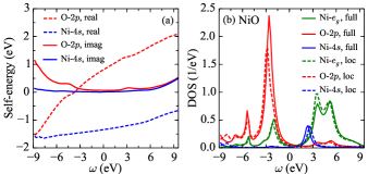
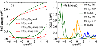
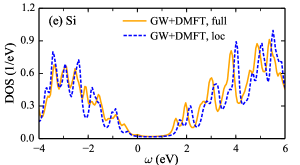
Figure 7: Effects of non-$d$-orbital vertex corrections to the self-energy (${\mathbf{\Sigma}}^{\mathrm{CC}}-{\mathbf{\Sigma}}^{\textit{GW}}$) on the full cell GW+DMFT results. (a) DMFT self-energy corrections to the O-$2p$ and Ni-$4s$ orbitals in NiO. (b) GW+DMFT ${\mathbf{k}}$-resolved DOS of NiO at the $\Gamma$ point, obtained by adding the self-energy correction to all impurity orbitals (“full”) or only the Ni-3d orbitals (“loc”). (c) DMFT self-energy corrections to O-$2p$ orbitals in SrMoO₃. (d) GW+DMFT local DOS of SrMoO₃, obtained by adding the self-energy correction to all impurity orbitals (“full”) or only the Mo-$4d$ orbitals (“loc”). (e) GW+DMFT local DOS of Si (HF reference), obtained by adding the self-energy correction to all impurity orbitals (“full”) or only the $3s3p$ orbitals within each Si atom (“loc”).

Lastly, in Fig. 7, we perform an analysis to understand the role of intermediate range interactions and vertex corrections that are now captured within our full cell GW+DMFT method but omitted in the usual downfolding based GW+DMFT treatments. In the systems studied here, one way in which this shows up is in quantitative corrections to the physics of the non-$d$ orbitals of metal and non-metal atoms, which are normally only treated at the DFT or GW level. As shown in Fig. 7(a) and (c), there are significant vertex corrections to the self-energies of the O-$2p$ and Ni-$4s$ orbitals in NiO and O-$2p$ orbitals in SrMoO₃ when using the full cell GW+DMFT method. Such vertex corrections lead to non-trivial effects on the spectral functions of the non-$d$ orbitals. For example, the peak position and intensity of O-$2p$ DOS is clearly changed in both NiO and SrMoO₃, when comparing the full and local (i.e., only Ni-$3d$ or Mo-$4d$) self-energy corrections (${\mathbf{\Sigma}}^{\mathrm{CC}}-{\mathbf{\Sigma}}^{\textit{GW}}$). Furthermore, because some non-$d$ orbitals are strongly hybridized with the $d$ orbitals, correcting the non-$d$ orbitals also modifies the $d$-orbital DOS in NiO and SrMoO₃. Meanwhile, in Fig. 7(e), we show that vertex corrections to the self-energies across two Si atoms within the impurity cell also lead to quantitative changes in the GW+DMFT DOS of Si (based on the HF reference). In summary, our full cell GW+DMFT provides vertex corrections to all orbitals, which is known to be necessary to achieve quantitative accuracy in many kinds of ab initio simulations Nilsson et al. (2017).

IV Conclusions

In this work, we introduced a full cell GW+DMFT formulation for the ab initio simulation of correlated materials. The primary strength of this approach is that it entirely avoids the problem of selecting a low-energy subspace, and consequently the uncontrolled errors introduced either by downfolding the effective interactions within the subspace, or via DFT double counting. The resulting method is then fully diagrammatically controlled and can easily treat all interactions, and provides a framework to apply advanced quantum chemistry methods to study correlated solids. We showed that full cell GW+DMFT can be applied to systems using impurity cells of up to 10 atoms in calculations of the spectral properties of Si, NiO, $\alpha$-Fe₂O₃ and SrMoO₃, obtaining for most quantities, results of good quantitative accuracy. By defining the impurity to comprise all orbitals in the AFM supercells of NiO and $\alpha$-Fe₂O₃, we also showed how the full cell approach can cleanly differentiate between different amounts of charge-transfer and Mott insulating character and the orbital character around the gap, as both metal and non-metal orbitals enter into the impurity problem on an equal footing. Overall, our calculations demonstrate the potential of the full cell GW+DMFT approach for studies of more complicated materials, en route towards a fully predictive theory of correlated materials.