Abstract

The research described herewith investigates detecting change points of means and of variances in a sequence of observations. The number of change points can be divergent at certain rate as the sample size goes to infinity. We define a MOSUM-based objective function for this purpose. Unlike all existing MOSUM-based methods, the novel objective function exhibits an useful “PULSE” pattern near change points in the sense: at the population level, the value at any change point plus 2 times of the segment length of the moving average attains a local minimum tending to zero following by a local maximum going to infinity. This feature provides an efficient way to simultaneously identify all change points at the sample level. In theory, the number of change points can be consistently estimated and the locations can also be consistently estimated in a certain sense. Further, because of its visualization nature, in practice, the locations can be relatively more easily identified by plots than existing methods in the literature. The method can also handle the case in which the signals of some change points are very weak in the sense that those changes go to zero. Further, the computational cost is very inexpensive. The numerical studies we conduct validate its good performance.

KEY WORDS: Double average ratios; MOSUM; multiple change-points detection; pulse pattern; visualization.

1. Introduction

Change points detection has attracted significant attention in a variety of research fields in decades (see, e.g. Page, (1954)). There are a number of methods available in the literature to detect sudden structure changes at certain points, that is, change points. For example Wu and Zhao, (2007) detected changes of mean in time series data for financial modeling, and Muggeo and Adelfio, (2011) identified genes associated with some diseases by applying a method of change points detection for means.

Methods designed for detecting change points in mean or variance with unknown number have been proposed in the literature. Almost all existing approaches for multiple change points could be roughly divided into two prevalent categories: model selection-based and hypothesis testing-based. For model selection-based approaches, as an example, Yao, (1988) firstly suggested a BIC type criterion for this purpose. More recently, regularization-based optimization approaches have been proposed. Yao and Au, (1989) proposed a penalized least squares-based approach for mean changes. A weighted least squares function-based method was suggested by Gao et al., (2018). Harchaoui and Levy-Leduc, (2010) proposed a LASSO-based approach. These approaches have been used in the cases with the fixed number of change points to obtain consistent estimators. For hypothesis testing-based methods, when detecting changes in means or variances, to facilitate the testing procedure by bisection algorithm a cumulative sum-based approach (CUSUM) that was firstly proposed by Page, (1954) has become a cornerstone in the later developments in such methodologies. Vostrikova, (1981) designed some tests for multiple changes through binary segmentation methods. To alleviate this difficulty caused by short spacings between change points or small jump magnitudes, Fryzlewicz, (2014) introduced an additional randomization step in the algorithm. Moving sum (MOSUM) or scan statistics are also popularly used to construct tests such as Bauer and Hackl, (1980) and Chu et al., (1995). In addition, Preuss et al, (2015) applied this methodology to handle multivariate time series data. Recently, Wu and Zhao, (2007) and Cao and Wu, (2015) discussed the limiting distributions of the maxima of MOSUM. The corresponding tests can well control their sizes, under the null hypothesis, close to the significance level.

Both classes of methodologies are usually efficient in estimation. As for their limitations, regularization-based estimations involving optimization algorithms have the problem of computational complexity, there are no results about the cases with divergent number of change points as the sample size goes to infinity. While hypothesis testing-based estimations have to benefit from bisection procedures to define test statistics for sequential testing, the resulting estimators are not consistent. The cases with divergent number of change points have not yet been discussed either. Using such procedures is partly because these methods do not have an implementable objective function to define a criterion to simultaneously detect all change points.

In this paper, we propose a novel approach for this purpose. Motivated by the idea of MOSUM, we define an objective function via a sequence of ridge ratios of moving averages. Note that to well identify change points, the key is how to make the values at the true change points(or nearby in certain sense) stand out. Unlike existing MOSUM-based methods and loss-function-based methods as well, the most distinguishing feature of the new criterion we will propose is that the defined objective function is discontinuous with an useful “PULSE” pattern near all change points: at the population level any change point plus 2 times of the segment length of moving average attains a local minimum tending to zero following by a local maximum going to infinity. Thus, this feature can very much make change points stand out and thus provide an efficient way to identify them. We will give a toy example to show this pattern in Section 2 when we describe the criterion construction. It is worthwhile to mention that because of the visualization nature, the plot of objective function can make all change points visualized and thus in practice it is very easy to implement with the help from plot. It is also computationally inexpensive without involving any optimality algorithm. We call this method a PULSE criterion. To show its usefulness, We will check how sensitive the criterion is to “weak changes” in the sense that some changes in the sequence of local means converge to, at a certain rate, a sequence without mean changes. As a generic methodology, it could be extended to handle other change points detection problems such as distributional changes (e.g. Pollak, (1987)), changes in regression models (e.g. Qu and Perron, (2007)) and change points of functional data (e.g. Berkes et al., (2009)). The research is ongoing. We also understand that it has the limitation to handle the problems with short spacings between two change points. This is because, to guarantee the estimation consistency, the segment length of the moving averages needs to be sufficiently large, which would contain more than one change point. We will have a brief discussion in Section 6.

The paper is organized as follows. In Section 2, we introduce the criterion construction, and investigate the estimation consistency. Section 3 contains the investigation on weak signals case where the magnitudes of the changes converge to zero at a certain rate. As an extension, Section 4 includes the detection of changes over variances. Some numerical studies are put in Section 5. Section 6 contains an illustrative application to the detection of mean changes. Section 7 includes some discussions for the merits and limitations of the method and some further research topics. All the technical proofs are presented in Appendix.

2. Methodological Development

2.1 Notations

Let $X_{1},...,X_{n}$ be independent one-dimensional random variables as

$X_{i}=\mu_{i}+\varepsilon_{i},1\leq i\leq n$,

where $\mu_{i}=E(X_{i})$ are the means. Assume that the sequence of all means follows a piecewise constant structure with $K+1$ segments. In other words, there are $K$ change points $1<z_{1}<z_{2}<...<z_{K}<n$ such that $\mu_{z_{k-1}+j}=\mu^{(k)}$, for $k=1,\cdots,K+1$ and $0\leq j\leq z_{k}-z_{k-1}-1$ where $z_{0}=0$ and $z_{K+1}=n$. For $k=1,...,K$, write $\beta_{k}=|\mu^{(k+1)}-\mu^{(k)}|$ for the (non-zero) difference in means between consecutive segments. The number $K$ can go to infinity as the sample size goes to infinity.

The goal of this research is to suggest a detection method for the locations of change points $\{z_{1},...,z_{K}\}$ in the data stream and the number $K$. To well estimate these consistently in a certain sense, we give some assumptions on the magnitudes of the mean changes $\{\beta_{k}:1\leq k\leq K\}$ and the lengths $z_{k+1}-z_{k}$ of segments. For notational convenience, write the minimum length of segments satisfies as $\alpha^{*}$:

$$\alpha^{*}:=\min_{0\leq k\leq K}\{z_{k+1}-z_{k}\}$$ (2.1)

and the minimum magnitudes of mean changes as $\nu$:

$$\nu:=\min_{1\leq k\leq K}\beta_{k}.$$ (2.2)

Write $1<\hat{z}_{1}\leq\hat{z}_{2}\leq...\leq\hat{z}_{K}<n-1$ as the estimated locations.

2.2 Criterion Construction

To achieve the goal discussed above, an objective function is constructed by the following steps. Consider the mean changes detection problem.

Difference of Moving Averages: To character the mean information, let $S(i)$ be the moving sum with length of $\alpha_{n}$ for every location $i$ as:

$$S(i)=\sum_{j=i}^{i+\alpha_{n}-1}\mu_{j}$$ (2.3)

where $\alpha_{n}$ is called the moving window. As the difference between two successive moving sums at the population level can show the mean change at its location $z_{k}$, we define $D(i)$ as: for $1\leq i\leq n-2\alpha_{n},$ if $2\alpha_{n}<\alpha^{*}$,

$$D(i) := {1\over\alpha_{n}}(S(i)-S(i+\alpha_{n}))$$ (2.4)

$$= {1\over\alpha_{n}}(\sum_{j=i}^{i+\alpha_{n}-1}\mu_{j}-\sum_{j=i+\alpha_{n}}^{i+2\alpha_{n}-1}\mu_{j})$$

For any fixed $k$, we have:

$$D(i)=\left\{\begin{array}[]{ll}{i-(z_{k}-\alpha_{n})\over\alpha_{n}}(\mu_{k+1}-\mu_{k}),&z_{k}-\alpha_{n}\leq i<z_{k},\\ {z_{k}+\alpha_{n}-i\over\alpha_{n}}(\mu_{k+1}-\mu_{k}),&z_{k}\leq i\leq z_{k}+\alpha_{n}\\ 0,&z_{k-1}+\alpha_{n}\leq i\leq z_{k}-\alpha_{n}.\end{array}\right.$$ (2.8)

This is because, when $z_{k-1}+\alpha_{n}\leq i\leq z_{k}-\alpha_{n}$, $S(i)=S(i+\alpha_{n})$. $D(i)$ attains a local maximum/minimum at $i=z_{k}$ for any $k$ with $1\leq k\leq K$ within the interval of length of $2\alpha_{n}$. Figure 1 presents the plot for visualizing the pattern. This is not a new idea while just the idea of MOSUM. However, as the local maximum/minimum values cannot be quantified to form an useful objective function, and more seriously, at the sample level, we can expect too many local maxima/minima due to the randomness oscillation, only identifying them makes no sense for the change points detection. Thus, we consider further construction to define an implementable objective function. Our idea is to construct a sequence of ridge ratios as an objective function that is of a pulse pattern within the space between a local maximum of $|D(i)|$ tending to infinity and a local minimum going to $0$ is $\alpha_{n}$ at the population level. However, it is easy to understand that as $D(i)$ and then the objective function at the sample level is relatively oscillating, it may cause difficulty to accurately determine the number of change points and locations. To make an objective function more smoothly at the sample level, we consider smoother averages than $D(i)$’s by doubly averaging below.

Doubly Averaging: The second round of averaging is to repeatedly use datum points in every average. To further make the values near the true change points stood out and more importantly, to establish a criterion for implementation, we use an idea of ridge ratio to construct an objective function. Denote $\tilde{D}(i)$ by the averages of $D(i)$ within the segments of length $\alpha_{n}$:

$$\tilde{D}(i)={1\over\alpha_{n}}\sum_{j=i}^{i+\alpha_{n}-1}D(j).$$ (2.9)

As the result, we have the following properties:

$$|\tilde{D}(i)|=\left\{\begin{array}[]{lll}0,&z_{k-1}+\alpha_{n}\leq i\leq z_{k}-2\alpha_{n};\\ {(i-z_{k}+2\alpha_{n}+1)\cdot(i-z_{k}+2\alpha_{n})\over\alpha_{n}^{2}}\beta_{k},&z_{k}-2\alpha_{n}<i\leq z_{k}-\alpha_{n};\\ {-i^{2}-\alpha_{n}i+2iz_{k}-i+z_{k}-z_{k}^{2}+\alpha_{n}z_{k}+{1\over 2}(\alpha_{n}^{2}-\alpha_{n})\over\alpha_{n}^{2}}\beta_{k},&z_{k}-\alpha_{n}<i<z_{k}-{\alpha_{n}\over 2}-{\sqrt{\alpha}_{n}};\\ ({3\over 4}-{\sqrt{\alpha}_{n}-1\over\alpha_{n}})\beta_{k},&i=z_{k}-{\alpha_{n}\over 2}-{\sqrt{\alpha}_{n}};\\ {-i^{2}-\alpha_{n}i+2iz_{k}-i+z_{k}-z_{k}^{2}+\alpha_{n}z_{k}+{1\over 2}(\alpha_{n}^{2}-\alpha_{n})\over\alpha_{n}^{2}}\beta_{k},&z_{k}-{\alpha_{n}\over 2}-{\sqrt{\alpha}_{n}}<i<z_{k}-{\alpha_{n}\over 2};\\ {3\over 4}\beta_{k},&i=z_{k}-{1\over 2}\alpha_{n};\\ {i^{2}+\alpha_{n}i-2iz_{k}+i-z_{k}+z_{k}^{2}-\alpha_{n}z_{k}-{1\over 2}(\alpha_{n}^{2}-\alpha_{n})\over\alpha_{n}^{2}}\beta_{k},&z_{k}-{\alpha_{n}\over 2}<i<z_{k}-{\alpha_{n}\over 2}+{\sqrt{\alpha}_{n}};\\ ({3\over 4}-{\sqrt{\alpha}_{n}-1\over\alpha_{n}})\beta_{k},&i=z_{k}-{\alpha_{n}\over 2}+{\sqrt{\alpha}_{n}};\\ {i^{2}+\alpha_{n}i-2iz_{k}+i-z_{k}+z_{k}^{2}-\alpha_{n}z_{k}-{1\over 2}(\alpha_{n}^{2}-\alpha_{n})\over\alpha_{n}^{2}}\beta_{k},&z_{k}-{\alpha_{n}\over 2}+{\sqrt{\alpha}_{n}}<i\leq z_{k};\\ {(-i+z_{k}+\alpha_{n}+2)(-i+1+\alpha_{n}+z_{k})\over\alpha_{n}^{2}}\beta_{k},&z_{k}<i\leq z_{k}+\alpha_{n};\\ 0,&z_{k}+\alpha_{n}<i\leq z_{k+1}-2\alpha_{n}.\end{array}\right.$$

where $\beta_{k}=|\mu_{k+1}-\mu_{k}|$. Thus,

$$\tilde{D}(i)\left\{\begin{array}[]{ll}>0,&z_{k}-3\alpha_{n}\leq i\leq z_{k},\\ =0,&otherwise.\end{array}\right.$$

Clearly, $\tilde{D}(i)$ attains local maxima at $z_{k}-{1\over 2}\alpha_{n}$ for each $k$ with $1\leq k\leq K$. The local maximizers of $\tilde{D}(i)$ plus ${1\over 2}\alpha_{n}$ are the locations of change points. Similarly as $D(i)$, the sequence $\tilde{D}(i)$ cannot be directly used to be an objective function either. Now we construct a sequence of ridge ratios as an objective function that is of a “pulse” pattern such that change points can be well identified.

Objective Function.   Consider the ratios between $\tilde{D}(i)$ and $\tilde{D}(i+{3\over 2}\alpha_{n})$. Define the ridge ratios $T(i)$ at the population level as

$$T(i)={{|\tilde{D}_{(}i)|+c_{n}}\over{|\tilde{D}(i+{3\over 2}\alpha_{n})|}+c_{n}},$$ (2.12)

where $c_{n}\to 0$ is a small value, to be selected later, to avoid the unstable terms $0/0$. In addition, for $i\in(z_{k-1}+\alpha_{n},z_{k}-2\alpha_{n})$, $|\tilde{D}(i)|=0$ and $|\tilde{D}(i+{3\over 2}\alpha_{n})|$ monotonically increases. For $i\in(z_{k}-2\alpha_{n},z_{k}-{1\over 2}\alpha_{n})$, $|\tilde{D}(i))|$ monotonically increases, and $|\tilde{D}(i+{3\over 2}\alpha_{n})|$ monotonically decreases. For $i\in(z_{k}-{\alpha_{n}\over 2},z_{k}+\alpha_{n})$, $|\tilde{D}(i+{3\over 2}\alpha_{n})|=0$ and $|\tilde{D}(i)|$ monotonically decreases. Then $c_{n}$ could also play a role of making $T(i)$ monotonic, to avoid the scenario where there are too many points tending to $0$. In summary, the following property could be easily justified: letting $\searrow$ and $\nearrow$ mean decreasing and increasing with respect to the index $i$; $\to 0$ and $\to\infty$ mean going to zero and infinity as the sample size $n\to\infty$,

$$T(i)=\left\{\begin{array}[]{ll}1,&z_{k-1}+\alpha_{n}\leq i\leq z_{k}-{7\over 2}\alpha_{n},\\ {c_{n}\over{|\tilde{D}(i+{3\over 2}\alpha_{n})|+c_{n}}}\searrow,&z_{k}-{7\over 2}\alpha_{n}<i<z_{k}-2\alpha_{n},\\ {c_{n}\over{|\tilde{D}(i+{3\over 2}\alpha_{n})|+c_{n}}}\to 0,&i=z_{k}-2\alpha_{n},\\ {|\tilde{D}(i)|+c_{n}\over|\tilde{D}(i+{3\over 2}\alpha_{n})|+c_{n}}\nearrow,&z_{k}-2\alpha_{n}<i<z_{k}-{\alpha_{n}\over 2},\\ {{|\tilde{D}(i)|+c_{n}}\over c_{n}}\to\infty,&i=z_{k}-{\alpha_{n}\over 2},\\ {|\tilde{D}(i)|+c_{n}\over c_{n}}\searrow,&z_{k}-{\alpha_{n}\over 2}<i<z_{k}+\alpha_{n},\\ 1,&z_{k}+\alpha_{n}\leq i<z_{k+1}-{7\over 2}\alpha_{n}.\end{array}\right.$$

Any true change point is just the index of a local minimum plus $2\alpha_{n}$. Based on this objective function, using the local minimizers to identify change points is convenient to implement. The toy example in Figure 1 shows the curve patterns of $D(i)$, $|\tilde{D}(i+\alpha_{n}/2)|$ and $T(i+2\alpha_{n})$ such that we have a better idea to understand why the pulse pattern of the objective function $T(i)$, rather than that of $D(i)$ or of $|\tilde{D}(i)|$, can be used to construct an useful criterion. Based on these properties, we can define its empirical version.

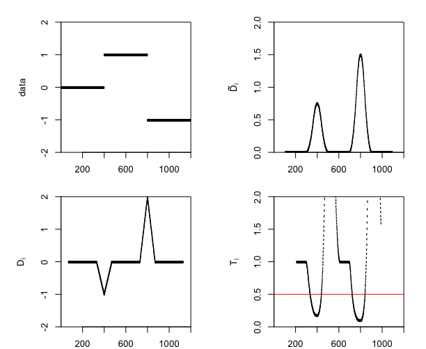
Figure 1: The plots at the population level

Sample Version. To define the objective function at the sample level, we can use the sample averages to estimate $D(i)$ and $\tilde{D}(i)$. Denote $\hat{S}(i)=\sum_{j=i}^{i+\alpha_{n}-1}X_{j}$ as the estimator of $S(i)$, $D_{n}(i)={1\over\alpha_{n}}(\hat{S}(i)-\hat{S}(i+\alpha_{n}))$ and $\tilde{D}_{n}(i)={1\over\alpha_{n}}\sum_{j=i}^{i+\alpha_{n}-1}D_{n}(j)$. The sample version of the objective function is then defined as: for $i=1,..,n-{7\over 2}\alpha_{n}$,

$$T_{n}(i)={{|\tilde{D}_{n}(i)|+c_{n}}\over{|\tilde{D}_{n}(i+{3\over 2}\alpha_{n})|}+c_{n}},$$ (2.14)

and the ridge value $c_{n}$ tends to $0$ at a certain rate specified later. We can see that $E\tilde{D}_{n}(i)=\tilde{D}(i)$.

Criterion: It is understandable that at the sample level, the objective function should be highly oscillating and there would be too many local minima. Thus, a natural idea is to restrict the search such that within each chosen interval, there is only one minimum of $T_{n}(i)$. We do this through a threshold $\tau$ with $0<\tau<1$. That is:

$\{i,1\leq i\leq n-{7\over 2}\alpha_{n}:T_{n}(i)<\tau\}$.

To make the search easily, we simply recommend $\tau=0.5$ as a compromised value as for large $\tau$ close to $1$, there would exist more local minima and for small $\tau$ close to $0$, there would exist less even no local minima. From the properties of $T_{n}(i)$ that can also be seen from the plot of Figure 1 heuristically, we can see that all these indices can be separated into several disjoint subsets each containing only one change point asymptotically. Therefore, we can separately within the disjoint subsets search for local minima. From the definition of $T(i)$ at the population level, we can see that the gap between two local minimizers must be larger than $2\alpha_{n}$. Due to the consistency of the involved estimators, we can see that there are $\hat{K}$ pairs $(m_{k},M_{k})$ where $m_{k}$ and $M_{k}$ are determined by $T_{n}(i)<0.5$ and $m_{k}$ satisfies that $T_{n}(m_{k}-1)\geq 0.5$ and $T_{n}(m_{k})<0.5$, and $T_{n}(M_{k})<0.5$ and $T_{n}(M_{k}+1)\geq 0.5$. Write $\hat{z}_{k}-2\alpha_{n}$ as the minimizer in each interval.

Theorem 2.1.

Assume that $X_{i}-EX_{i}$ are independent identically distributed random variables and ${\alpha^{*}\over{n^{1/2}(\log n)^{2}}}\rightarrow\infty$, where $\alpha^{*}$ is the minimum number of samples between any two change points. The tuning parameter $c_{n}$ and the segment length $\alpha_{n}$ satisfies that ${c_{n}\over{\sqrt{\log n\over\alpha_{n}}}}\rightarrow\infty$, ${n^{1/4}\log n\over{\sqrt{\alpha}_{n}}}\rightarrow 0$, and ${\alpha^{*}\over\alpha_{n}}\rightarrow\infty$.

(1) When $K$ is known, then the estimators $\{\hat{z}_{1},...,\hat{z}_{K}\}$ have: $\lim_{n\rightarrow\infty}\Pr\{\max_{1\leq k\leq K}{|{\hat{z}_{k}-z_{k}\over\alpha_{n}}|}<\epsilon\}\rightarrow 1$, for every $\epsilon>0$.

(2) When $K$ is fixed but unknown, then $\hat{K}=K$ with a probability going to one and the estimators $\{\hat{z}_{1},...,\hat{z}_{\hat{K}}\}$ have: $\lim_{n\rightarrow\infty}\Pr\{\max_{1\leq k\leq K}{|\hat{z}_{k}-z_{k}|\over\alpha_{n}}<\epsilon\}\rightarrow 1$, for every $\epsilon>0$.

(3) When $K$ is divergent at the rate satisfying ${n\over\alpha^{*}K}\rightarrow\infty$ and unknown, the results are the same as those in (2).

Remark 1.

These conditions are based on the following observations. First, we will prove that $\tilde{D}_{n}(i)-\tilde{D}(i)$ converges to $0$ at a rate of order $\sqrt{\log n\over\alpha_{n}}$. Then the ridge $c_{n}$ should be a dominating term in every $T_{n}(i)$, which converges to $0$ at a rate slower than that of $\tilde{D}_{n}(i)-\tilde{D}(i)$. Such a ridge can help $T_{n}(i)$ keep the property of $T(i)$ asymptotically. We will show this in the proofs of the theorems in Appendix.

In the estimation, the ridge $c_{n}$ needs to be selected. We will recommend a choice for practical use in the numerical studies. To guarantee the estimation consistency, the bandwidth $\alpha_{n}$ should not be too small such that the averages can be close to the corresponding means. Thus, for the paradigms with very short spacing, our method, similarly as any MOSUM-based methods, may not perform well. This deserves a further study.

Remark 2.

In the third part of this theorem, we allow the number of change points divergent. To the best of our knowledge, there are not many proposals in the literature to discuss this problem. Zou et al., (2019) developed a cross-validation estimation scheme, the estimation consistencies of the number and locations of change points were not provided. In contrast, the proposed criterion is of visualization nature and without resampling approximation, the determination is rather convenient and computationally inexpensive.

3. Weak signals case

In this section, we extend the criterion to handle weak signal scenarios. The term “weak signals” in this section means that the magnitudes of some changes converge to $0$ at a certain rate as the sample size goes to infinity. We also call such models as local models. Consider the sequence of models as, for $1\leq k\leq K$:

$$X_{i}=\mu+\beta_{z_{k}}\mathbb{I}\{i\geq z_{k}\}+\epsilon,$$ (3.1)

where $z_{k}$ are the locations of change points. $\beta_{z_{k}}$ are the change magnitudes, which would converge to $0$ as $n$ goes to infinity. Denote $\beta_{z}=\min_{1\leq k\leq K}\beta_{k}$. We have the following results.

Theorem 3.1.

Assume that $X_{i}-EX_{i}$ are independent identically distributed random variables and ${\alpha^{*}\over{n^{1/2}(\log n)^{2}}}\rightarrow\infty$. The tuning parameter $c_{n}$ and $\alpha_{n}$ satisfies that ${c_{n}\over{\sqrt{\log n\over\alpha_{n}}}}\rightarrow\infty$, ${n^{1/4}\log n\over{\sqrt{\alpha}_{n}}}\rightarrow 0$, and ${\alpha^{*}\over\alpha_{n}}\rightarrow\infty$. For the sequence of local models in (3.1), under the conditions in Theorem 2.1, if ${\log\alpha_{n}}^{1/5}\beta_{z}\to\infty$, we have $\lim_{n\rightarrow\infty}\Pr\{\hat{K}=K\}=1$ and $\lim_{n\rightarrow\infty}\Pr\{\max_{1\leq k\leq K}{|\hat{z}_{k}-z_{k}|\over\alpha_{n}}<\epsilon\}=1$, for every $\epsilon>0$.

4. Extension

In this section, we extend the criterion to handle detecting change points in variances. Consider second moments of $X_{i}$’s that are generated from the following model:

$$X_{i}=\mu+\varepsilon_{i},1\leq i\leq n,$$ (4.1)

where $\mu$ is an unknown mean and $E(\varepsilon)=0$, $Var(\varepsilon)=\sigma^{2}_{(i)}$. Similarly, we assume that the variances follow a piecewise constant structure with $K+1$ segments. In other words, there are $K$ change points $1<z_{1}<z_{2}<...<z_{K}<n-1$ such that, for any $k$ with $0\leq k\leq K$,

$$Var(\varepsilon_{z_{k}+1})=...=Var(\varepsilon_{z_{k+1}})=\sigma^{2}_{k}.$$ (4.2)

As before, define $z_{0}=0$ and $z_{K+1}=n$. At population level, we can similar define $D(i)$ and $\tilde{D}(i)$ as follows.

$$D(i)=\sigma_{(i)}-\sigma_{(i+\alpha_{n})}$$

and

$$\tilde{D}(i)={1\over\alpha_{n}}\sum_{j=i}^{i+\alpha_{n}-1}D(j).$$

Similarly, at the sample level, as the mean is unknown but all the same, we can estimate $\mu$ by sample mean.

Let

$$\hat{\sigma}^{2}_{(i)}={1\over\alpha_{n}}\sum_{t=i}^{t=i+\alpha_{n}-1}(X_{t}-{1\over n}\sum_{j=1}^{j=n}X_{j})^{2}.$$ (4.3)

and define similarly $D_{n}(i)$ and $\tilde{D}_{n}(i)$ as the difference of moving averages and the average of $D_{n}(j)$’s:

$$D_{n}(i)=\sqrt{\hat{\sigma}^{2}_{(i)}}-\sqrt{\hat{\sigma}^{2}_{(i+\alpha_{n})}},$$ (4.4)

$$\tilde{D}_{n}(i)={1\over\delta_{n}}\sum_{j=i}^{i+\delta_{n}}D_{n}(j).$$ (4.5)

Finally, we take ratios of $\tilde{D}(i)$ to acquire the statistics,$T(i)$ we will use to estimate change points. That is:

$$T_{n}(i)={{|\tilde{D}_{n}(i)|}+c_{n}\over{|\tilde{D}_{n}(i+{3\over 2}\alpha_{n})|}+c_{n}}.$$ (4.6)

Theorem 4.1.

Assume that $X_{i}-\mu$ are independent distributed random variables and $\alpha^{*}$, $c_{n}$ and $\alpha_{n}$ satisfy the same conditions as in Theorem 2.1.

(1) When $K$ is given, then the estimators $\{\hat{z}_{1},...,\hat{z}_{K}\}$ have: $\lim_{n\rightarrow\infty}\Pr\{\max_{1\leq k\leq K}{|{\hat{z}_{k}-z_{k}\over\alpha_{n}}|}<\epsilon\}\rightarrow 1$, for every $\epsilon>0$.

(2) When $K$ is unknown but fixed, then $\hat{K}=K$ with a probability going to one and the estimators $\{\hat{z}_{1},...,\hat{z}_{\hat{K}}\}$ have: $\lim_{n\rightarrow\infty}\Pr\{\max_{1\leq k\leq K}{|\hat{z}_{k}-z_{k}|\over\alpha_{n}}<\epsilon\}\rightarrow 1$, for every $\epsilon>0$.

(3) When $K$ is divergent at the rate satisfying ${n\over\alpha^{*}K}\rightarrow\infty$ and unknown, the results are identical to those in (2).

Remark 3.

This theorem told us that our method could be extended to scenarios for detecting change point in variance. The only difference between mena change scenario and variance scenario is that the former is based on first monment while the later is based on second monment. The proof of this result is very similar to that for mean. Some conditions on forth monment of the sample will also be considered.

5. Simulation

To evaluate the performance of our proposed Thresholding Double Average Ratio procedure which utilizes the property of average and ratio for identifying the locations and the number of change points, we mainly run the simulations with the other competing procedures that have also been considered in Fryzlewicz, (2014), where we use the suggested sSIC-method for wild binary segmentation. Precisely, the methods are CumSeg as described in Muggeo and Adelfio, (2011) , SMUCE as described in Frick et al., (2014), as well as WBS as considered in Fryzlewicz, (2014). For both standard change point scenario and local alternatives situation, the implementation of detection requires the choice of paramters, $\alpha_{n}$, $\tau$ and $c_{n}$. In order to avoid getting trouble in choosing parameter, we are to propose a data-driven algorithm for automatically selecting some parameters based on data. The specific algorithm have been given in Algorithm 1. Another important thing in practice is to choose an appropriate thresholding. Threshold value will not be decided by data as we can give a expanation in theory. Theoretically, threshold should be $0$ becasue our statistics drop from 1 to $0$ at change point. However, in our simulation and real data, there is always some error that we can’t avoid. Thus, we will relax the strict requirement and take it as a larger value. Here we use 0.5 as our choice. We have used normal distribution with mean changing from 1 to 4. As could be seen from Picture 3, the statistics drop below 0.5 clearly and thus the change points is the index attaching the minimum points.

Input: $X\in\mathcal{R}^{n\times 1}$

1 Take $\alpha_{n}=n^{0.6}/3$, $\tau=0.5$, $c_{n}=\sqrt{\log n\over\alpha_{n}}$and then perform the Double Average Ratio steps directly to acquire a preliminary estimation $\hat{z}_{i},$ for $i=1,...,k.$;

2

3Calculate the variance for each segementation $\hat{\sigma}_{i},i=1,...,k,$ and average them, $\bar{\sigma}={{1\over k}\sum_{i=1}^{k}\sigma_{i}}.$;

4 Take $c_{n}=\sqrt{\log\over\alpha_{n}}*{1\over\bar{\sigma}}$, and perform TMAR construction steps again. ;

5 Estimate $\hat{z}_{i}$ based on parameters we select in step 3.;

Output: $\hat{z}_{i}$

Algorithm 1 How to estimate change points

For each example, 1000 replications is used to approximate the distribution of $\hat{K}-K$, where $\hat{K}_{n}$ is the estimated number of change points.

5.1 Mean

Part 1: CP model

CP Model: Both the number and locations of change points are fixed. We adopt the blocks setting which is wildly used in the literature (Fryzlewicz, (2014)). Specifically, $K_{n}=11$ and change points at 161, 323, 485, 638, 801, 967, 1132, 1299, 1465, 1632, 1794, and the values between 1, 3, 2, -1, 1, 3, 2, 5, 1, -2, 3, 0.

Detecting mean shift in a univariate observations has been widely discussed in the literature. In this section, two different change point model will be both considered. Four scenarios of error distribution will also be taken into account:

• (i) $\varepsilon_{i}\backsim^{iid}N(0,1)$,

• (ii)$\varepsilon_{i}\backsim^{iid}N(0,3)$,

• (iii) $\varepsilon_{i}\backsim^{iid}7*Uniform(-1,1)$,

• (iv)$\varepsilon_{i}\backsim^{iid}3*t_{3}$,

where $t_{v}$is the Student’s t-distribution with degree of freedom $v$. The model we simulate could be represented as the following form:

$$X_{i}=\mu_{i}+\varepsilon_{i}.$$ (5.1)

There are two models we will take into consideration. The first one is standard change point model which is usually used in the literature. While the second one is CP alternative model, which considers the weak magnitude signal for the change.

In this part, standard change point model which is used in the literature is considered, which means both the number and locations of change point are fixed, where we set $n=2048$. The signal function $\mu_{i}$s are chosen as a piecewise constant function with $K=11$. Table 1 compares the performance of TMAR and other competing procedures under different error settings. All the algorithms were run on the same data matrices and the the distribution of $\hat{K}-K$ is reported.

It can be seen from table 1 that TMAR has a competitive performance for the change point estimation task. When $\sigma=1$, the other methods would perfoamce better than us. However, when $\sigma^{2}=3$, all the other methods would underestimate the number of change points. Though our method would also perform not so good, it is better than the others. When error type change from normal to some other distribution, our method perform obviously better than the others. When the error follows a uniform distribution, other methods would also underestimate change points number, but TMAR perform more stable compared with them. For $t$-distribution, cumSeg seriously underestimated change points while WBS and SMUCE would overestimate. They all doesn’t work at all. Our method in some extent over estimate, but perform more stable than the others. Actually it is easy to understand. As in our setting the magnitude between change points are small, all the methods might perform not as good as we image. However, our method would still perform more stable than the others.

Part 2: CP local alternative model

CP Alternative Model: In this model, we take magnitude smaller. Specifically, $K=11$ and change points at 161, 323, 485, 638, 801, 967, 1132, 1299, 1465, 1632, 1794, and the values between 0, 0.7, 0, -0.7, 0.7, 0 , 2, 2.7, 0, -2.7, -2, 0. In this section, we are considering the following four types of error distribution.

• (i) $\varepsilon_{i}\backsim^{iid}N(0,1)$,

• (ii)$\varepsilon_{i}\backsim^{iid}N(0,3)$,

• (iii) $\varepsilon_{i}\backsim^{iid}7*Uniform(-1,1)$,

• (iv)$\varepsilon_{i}\backsim^{iid}t_{3}$,

We are interested in the performance of our method and the others when facing the scenario of weak signal. In this situation, we have also presented the result of multiple change point detection. The distribution of $\hat{K}-K$ have been reported in Table 2, displaying the error between the truth and the estimated location.

From table 2, we can observe that our method perform obviously better than the other methods. Under the local alternative model, cumSeg, WBS and SMUCE could not estimate accurately, and even they couldn’t detect the existence of change point. However, our approach can still work very well in terms of the number of change point. When the error type is normal distribution with $\sigma^{2}=3$, TMAR perform not as good as we image, but still more accurate than the other competitiors. It can be seen that our procedure is more robust than the other procedures from an overall view. Actually this result is easy to understand. all the other approaces have not considered the local alternatives. They all assumed that the signal is strong enough. It is not always that case. When the signal is weak, they could not work at all.

We now suggest an iterative algorithm to detect change points, which could be used in the short spacing scenarios. Note that in our method, the segment length must be larger than $3\alpha_{n}$ where $\alpha_{n}=O(n^{0.6})$. When the spacings between two change points is short, the length may be larger than the spacing and the change point within the segment cannot be found out. To attenuate the severity of this difficulty, the iterative algorithm is as follows.

1

Input: $X\in\mathcal{R}^{n\times 1}$

2

3Start with the original data as the initial segement.;

4

5Perform Algorithm 1 on the segementations and get an estimation of change points for each segementation.;

6

7For each segementation in the last step perform Algorithm 1 untill there is no point of $T_{n}(i)$ found lower than $0.5$.;

8

Output: All $\hat{z}_{i}$

Algorithm 2 How to estimate change points for short spacing

5.2 Variance

The idea of detecting changes in mean can be easily extended to the variance change point problem. Similarly, four scenarios of error distribution will also be taken into account in this part:

• (i) $\varepsilon_{i}\backsim^{iid}N(0,1)$,

• (ii)$\varepsilon_{i}\backsim^{iid}N(0,3)$,

• (iii) $\varepsilon_{i}\backsim^{iid}7*Uniform(-1,1)$,

• (iv)$\varepsilon_{i}\backsim^{iid}3*t_{3}$,

where $t_{v}$is the Student’s t-distribution with degree of freedom $v$. However, the model we simulate is different from the mean, which could be represented as the following form:

We will take the model:

$$X_{i}=\sigma_{i}\varepsilon_{i}.$$ (5.2)

Similar to the last part, we will compare the performance of number of change points of four methods including SUMCE, BS which was introduced in last part and PELT which was considered in Killick et al., (2012). In this part, standard change point model which is used in the literature is considered, which means both the number and locations of change point are fixed, where we set $n=2048$. The signal function $\mu_{i}$s are chosen as a piecewise constant function with $K=11$. Table 3 compares the performance of TMAR and other competing procedures under different error settings. All the algorithms were run on the same data matrices. We report the distribution of $\hat{K}-K$.

Table 3 gives the results of different error settings. Again we find that the performance of TMAR is very encouraging on all performance measures. For all situations, SMUCE and BS doesn’t work at all for variance change point situation. Under normal distribution with $\sigma=1$, PELT is more accurate than our procedures however, when $\sigma^{2}=3$ our approach is more precise than PELT. When the error typr change to uniform distribution and t-distribution, our method performs more robust than PELT. All in all, our approach could deal with variance change point problem more precisely and robust.

6. Real Data Examples

Consider an Array CGH data set, which shows aberrations in genomic DNA. The observations are normalized glioblastoma profiles from the data set of Bredel et al., (2005). We now detect regions on which the observations jump from $0$. Compute $T_{n}(i)$ about the array CGH profile of chromosome 13 in GBM31. The threshold $\tau=0.5$ and ridge $c_{n}$ are selected as before. In Figure 2, we plot the original data, $D_{n}(i)$, $\tilde{D}_{n}(i)$ and $T_{n}(i)$. From $D_{n}(i)$, we may see that the magnitudes of changes are small except for a point between $500$ and $600$, which is also smaller than $0.5$. $\tilde{D}_{n}(i)$ also shows this pattern, but the point is more stood out although the magnitude is still small about $0.4$. The plot of $T_{n}(i)$ presents a curve to clearly indicate that this point can be regarded as a change point. $T_{n}(i)$ also suggests the location of the change point is the number $579$. From all four plots, the determination of this location would be reliable.

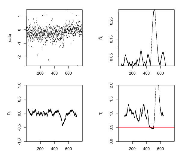
Figure 2: The plots for the Array CGH data

7. Discussion

This paper has developed a new method to estimate the change point location. We have propoesed several setps procedure to eatimate the location and the number of change point at the same time. Our approach is easy to implement and more direct. In addition, our approach could be extended to a more general case besides mean and variance case which was considered in this paper. For example, our approach might be used to detect change point in distribution by the information of the difference between empirical distribution function. But it is difficult to deal with a sequence of the functions. Besides, our approach might also be applied to multivariate data which was considered in Matteson and James, (2014). However a reasonable measurement is not easy to find. Wang and Samworth, (2018) clarify a high dimensional change point detection method. Under some conditions, our method might also be used to deal with change point detection problem in high dimensional data. But when coping with high dimensional data it is difficult to solve with caculation problem. More general, when coping with change point problem in functional data mentioned in Berkes et al., (2009), our approach might also work but perhaps, some other conditions need to be added.

As we commented before, this method has the limitation to handle the short spacing issue. As an attempt, we once considered an iterative algorithm to partly alleviate this determination difficulty. The basic idea is that after performing the algorithm, the locations of some change points have been identified and estimated, we then perform the algorithm again with the samples between any two consecutive locations to see whether there are other change points. In such a procedure, the sample sizes could be very much reduced, the segment lengths could then be much shorter. A small numerical study showed that some more locations are regarded as change points. However, as the length is shorter, the corresponding objective function became oscillating such that the algorithm could produce an over-estimation. The numerical study showed that this phenomenon became more obvious with larger variance. Therefore, how to combine this method with existing methods that can handle short spacing issue is an interesting topic in a further study.

8. Appendix

In this section, we present the proofs of the theoretical results.

8.1 Appendix A: Two lemmas

We give two lemmas first.

Lemma 1.

Assume that $X_{i}-EX_{i}$ are independent identically distributed random variables and ${n^{1/4}\log n\over{\sqrt{\alpha}_{n}}}\rightarrow 0$,

$$\Pr\{\max_{1\leq i\leq n}\Big{|}|\tilde{D}_{n}(i)|-|D(i)|\Big{|}>\tau_{n}\}=o(1)$$ (A.1)

where $\tau_{n}=O(\sqrt{\log n\over\alpha_{n}})$.

Proof of Lemma 1 We first rewrite $\tilde{D}_{n}(i)$ as a sum of independent variables:

$$\tilde{D}_{n}(i) = {1\over\alpha_{n}^{2}}\bigg{\{}\sum_{j=i}^{i+\alpha_{n}-1}(j-i+1)X_{j}+\sum_{i+\alpha_{n}}^{i+2\alpha_{n}-1}(3\alpha_{n}-2j+2i-2)X_{j}$$ (A.2)

$$+\sum_{i+2\alpha_{n}}^{i+3\alpha_{n}-1}(3\alpha_{n}-j+i-1)X_{j}\bigg{\}}.$$

Then the variance of $\tilde{D}_{n}(i)$ equals, for a constant $C>0$:

$$Var\bigg{\{}{1\over\alpha_{n}^{2}}(\sum_{j=i}^{i+\alpha_{n}-1}(j-i+1)X_{j}+\sum_{j=i+\alpha_{n}}^{i+2\alpha_{n}-2}(2i+3\alpha_{n}-2j-2)X_{j}$$ (A.3)

$$+\sum_{i+2\alpha_{n}-1}^{i+3\alpha_{n}-2}(i+3\alpha_{n}-j-1)X_{j})\bigg{\}}$$

$$= {Var(X_{1})\over\alpha_{n}^{4}}(\sum_{i=1}^{\alpha_{n}}2*i^{2}+\sum_{h=1}^{\alpha_{n}}(3\alpha_{n}-2h)^{2}):={C^{2}\over\alpha_{n}}=\sigma_{n}^{2}.$$

It is obvious that the variance of $\tilde{D}(i)$ is then free of the index $i$ with $\sigma_{n}=C/\sqrt{\alpha}_{n}$. In addition, as $\tilde{D}_{n}(i)$ is a weighted sum of $\{X_{i}\}_{i=1}^{n}$, we then further rewrite it. Define a weight function $w_{n}(t,j)$ as denoting $[nt]$ as the largest integer that is smaller or equal to $[nt]$,

$$w_{n}(t,j) =\operatorname{I}\{[nt]\leq j\leq[nt]+\alpha_{n}-1\}{(j-[nt]+1)\over\alpha_{n}^{2}}$$

$$\quad+\operatorname{I}\{[nt]+\alpha_{n}\leq j\leq[nt]+2\alpha_{n}-1\}{(3\alpha_{n}-2j+2[nt]-2)\over\alpha_{n}^{2}}$$

$$\quad+\operatorname{I}\{[nt]+2\alpha_{n}\leq j\leq[nt]+3\alpha_{n}-1\}{(3\alpha_{n}-j+[nt]-1)\over\alpha_{n}^{2}},$$

where $\operatorname{I}\{B\}$ denotes indicator function of set $B$. As for evert $i$ there exists $t_{i}\in(0,1)$ such that $i=[nt_{i}]$, we have

$$w_{n}(t_{i},j) =\operatorname{I}\{[nt_{i}]\leq j\leq[nt_{i}]+\alpha_{n}-1\}{(j-i+1)\over\alpha_{n}^{2}}$$ (A.4)

$$\quad+\operatorname{I}\{[nt_{i}]+\alpha_{n}\leq j\leq[nt_{i}]+2\alpha_{n}-1\}{(3\alpha_{n}-2j+2[nt_{i}]-2)\over\alpha_{n}^{2}}$$

$$\quad+\operatorname{I}\{[nt_{i}]+2\alpha_{n}\leq j\leq[nt_{i}]+3\alpha_{n}-1\}{(3\alpha_{n}-j+[nt_{i}]-1)\over\alpha_{n}^{2}}.$$

$\tilde{D}_{n}(i)$ can then be rewritten as $\tilde{D}_{n}(i)=\sum_{j=1}^{n}w_{n}(t_{i},j)X_{j}$. Then $\tilde{D}_{n}(i)-\tilde{D}(i)=\sum_{j=1}^{n}w_{n}(t_{i},j)(X_{j}-E(X_{j}))$. Thus we have

$$\frac{\tilde{D}_{n}(i)-\tilde{D}(i)}{\sigma_{n}}=\sum_{j=1}^{n}{w_{n}(t_{i},j)\over\sigma_{n}}(X_{j}-E(X_{j}))$$

Let $\tilde{w}_{n}(t_{i},j)={w_{n}(t_{i},j)\over\sigma_{n}}$, $Y_{n}(t_{i})={\tilde{D}_{n}(i)-\tilde{D}(i)/\sigma_{n}}$ and $e_{j}=X_{j}-E(X_{j})$. Then we have that

$$Y_{n}(t_{i})=\sum_{j=1}^{n}\tilde{w}_{n}(t_{i},j)e_{j},$$ (A.5)

where $\tilde{w}_{n}(t_{i},j)$ can be seen as a special case of Equation (18) in Wu and Zhao, (2007). In addition, define $\Omega_{n}(t_{i})=|\tilde{w}_{n}(t_{i},1)|+\sum_{j=2}^{n}|\tilde{w}_{n}(t_{i},j)-\tilde{w}_{n}(t_{i},j-1)|$ and $\Omega_{n}=\max_{1\leq i\leq n}\{\Omega_{n}(t_{i})\}$. Some elementary calculations lead to

$$\Omega_{n}(t_{i})={4\alpha_{n}+3\over\alpha_{n}^{2}\sigma_{n}}.$$ (A.6)

As $\Omega_{n}(t_{i})$ is free of $i$ and then $\Omega_{n}={4\alpha_{n}+3\over\alpha_{n}^{2}\sigma_{n}}$. The application of Theorem 3 in Wu, (2007) and Equation (6) in Wu and Zhao, (2007) yield that there exists a Gaussian process below with the standard Brownian motion $\mathbb{B}(\cdot)$,

$$Y_{n}^{*}(t_{i})=\sum_{j=1}^{n}\tilde{w}_{n}(t_{i},j)\sqrt{Var(X_{1})}\{\mathbb{B}(j)-\mathbb{B}(j-1)\}$$ (A.7)

such that almost surely for all $i$

$$|Y_{n}(t_{i})-Y_{n}^{*}(t_{i})|\leq o({\Omega_{n}(t_{i})n^{1/4}\log n}),$$ (A.8)

and then

$$\max_{1\leq i\leq n}|Y_{n}(t_{i})-Y_{n}^{*}(t_{i})|=o({\Omega_{n}n^{1/4}\log n}).$$ (A.9)

This yields that almost surely

$$\max_{1\leq i\leq n}|Y_{n}(t_{i})| =\max_{1\leq i\leq n}|Y_{n}(t_{i})-Y_{n}^{*}(t_{i})+Y_{n}^{*}(t_{i})|$$ (A.10)

$$\leq\max_{1\leq i\leq n}|Y_{n}^{*}(t_{i})|+\max_{1\leq i\leq n}|Y_{n}(t_{i})-Y_{n}^{*}(t_{i})|$$

$$\leq\max_{1\leq i\leq n}|Y_{n}^{*}(t_{i})|+o(\Omega_{n}n^{1/4}\log n),$$

and

$$\max_{1\leq i\leq n}\Big{|}|\tilde{D}_{n}(i)|-|\tilde{D}(i)|\Big{|}/\sigma_{n} \leq\max_{1\leq i\leq n}\Big{|}\tilde{D}_{n}(i)-\tilde{D}(i)\Big{|}/\sigma_{n}$$ (A.11)

$$=\max_{1\leq i\leq n}\Big{|}Y_{n}(t_{i})\Big{|}$$

$$\leq\max_{1\leq i\leq n}|Y_{n}^{*}(t_{i})|+o(\Omega_{n}n^{1/4}\log n).$$

Due to the fact $\sigma_{n}=O(1/\sqrt{\alpha}_{n})$ and the result in (A.6), we can see that $\Omega_{n}={4\alpha_{n}+3\over\alpha_{n}^{2}\sigma_{n}}=O(1/\sqrt{\alpha}_{n})$. By the condition ${n^{1/4}\log n\over\sqrt{\alpha}_{n}}\rightarrow 0$, we have for any $\tau_{n}$

$$\Pr\{\max_{1\leq i\leq n}\Big{|}|\tilde{D}_{n}(i)|-|\tilde{D}(i)|\Big{|}>\tau_{n}\} =\Pr\{\max_{1\leq i\leq n}\Big{|}|\tilde{D}_{n}(i)|-|\tilde{D}(i)|\Big{|}/\sigma_{n}>\tau_{n}/\sigma_{n}\}$$ (A.12)

$$\leq\Pr\{\max_{1\leq i\leq n}\Big{|}Y_{n}^{*}(t_{i})\Big{|}+o({n^{1/4}\log n\over\sqrt{\alpha}_{n}})>\tau_{n}/\sigma_{n}\}$$

$$\leq\Pr\{\max_{1\leq i\leq n}\Big{|}Y_{n}^{*}(t_{i})\Big{|}+1>\tau_{n}/\sigma_{n}\}.$$

From (A.7), we have

$$\operatorname{Var}(Y_{n}^{*}(i))={Var(X_{1})\over\sigma_{n}^{2}\alpha_{n}^{4}}(\sum_{i=1}^{\alpha_{n}}2*i^{2}+\sum_{h=1}^{\alpha_{n}}(3\alpha_{n}-2h)^{2})=1$$ (A.13)

In other words, $Y_{n}^{*}(t_{i})$ follows the standard normal distribution, and thus with an application of Proposition 2.1.2 in Roman, (2017), we have, for large $\tau_{n}/\sigma_{n}$,

$$\Pr\{\max_{1\leq i\leq n}\Big{|}Y_{n}^{*}(t_{i})\Big{|}+1>\tau_{n}/\sigma_{n}\}\leq n\max_{1\leq i\leq n}\Pr\{\Big{|}Y_{n}^{*}(t_{i})\Big{|}+1>\tau_{n}/\sigma_{n}\}$$ (A.14)

$$=n\Pr\{\Big{|}Y_{n}^{*}(t_{1})\Big{|}>\tau_{n}/\sigma_{n}-1\}$$

$$\leq n/({\tau_{n}\over\sigma_{n}}-1)\exp\{-{1\over 2}({\tau_{n}\over\sigma_{n}}-1)^{2}\}.$$

Taking $\tau_{n}/\sigma_{n}={\sqrt{2\log n}}+1$, we have as $n\rightarrow\infty$

$$n/({\tau_{n}\over\sigma_{n}}-1)\exp\left\{-{1\over 2}({\tau_{n}\over\sigma_{n}}-1)^{2}\right\} =\exp\left\{\log n-\log{\sqrt{2\log n}}-\log n\right\}$$

$$=\sqrt{1\over 2\log n}\rightarrow 0.$$

That is when $\tau_{n}=\sigma_{n}({\sqrt{2\log n}}+1)=O(\sqrt{\log\alpha_{n}}/\sqrt{\alpha_{n}})$ and $n\rightarrow\infty$, we have

$$\Pr\{\max_{1\leq i\leq n}\Big{|}|\tilde{D}_{n}(i)|-|\tilde{D}(i)|\Big{|}>\tau_{n}\}\leq\sqrt{1\over 2\log n}\rightarrow 0.$$ (A.15)

This means that $\max_{1\leq i\leq n}\Big{|}|\tilde{D}_{n}(i)|-|\tilde{D}(i)|\Big{|}=O_{p}(\sqrt{\log n\over\alpha_{n}}).$ We complete the proof of Lemma 1.

For the consistency of the estimated change points defined in the criterion, we first give the detailed computation of $\tilde{D}(i)$. It is easy to see that

$$|\tilde{D}(i)|=\left\{\begin{array}[]{lll}0,&z_{k-1}+\alpha_{n}\leq i\leq z_{k}-2\alpha_{n};\\ {1+\cdots+(i-(z_{k}-2\alpha_{n}))\over\alpha_{n}^{2}}\beta_{k},&z_{k}-2\alpha_{n}<i\leq z_{k}-\alpha_{n};\\ {{[(i-(z_{k}-\alpha_{n}-1))+\cdots+\alpha_{n}]}+{[(\alpha_{n}-1)+\cdots+(\alpha_{n}-(i-(z_{k}-\alpha_{n})))]}\over\alpha_{n}^{2}}\beta_{k},&z_{k}-\alpha_{n}<i\leq z_{k}-{\alpha_{n}\over 2};\\ {{[(z_{k}-i+2)+\cdots+\alpha_{n}]}+{[(\alpha_{n}-1)+\cdots+(\alpha_{n}-(z_{k}-i+1))]}\over\alpha_{n}^{2}}\beta_{k},&z_{k}-{\alpha_{n}\over 2}<i\leq z_{k};\\ {1+\cdots+((z_{k}+\alpha_{n})-i+1)\over\alpha_{n}^{2}}\beta_{k},&z_{k}<i\leq z_{k}+\alpha_{n};\\ 0,&z_{k}+\alpha_{n}<i\leq z_{k+1}-2\alpha_{n}.\par\end{array}\right.$$

From this formula, we have a more detailed calculation that will be used in the proof of Lemma 2 and Theorem 2.1:

$$|\tilde{D}(i)|=\left\{\begin{array}[]{llll}0,&z_{k-1}+\alpha_{n}\leq i\leq z_{k}-2\alpha_{n};\\ {(i-z_{k}+2\alpha_{n}+1)\cdot(i-z_{k}+2\alpha_{n})\over\alpha_{n}^{2}}\beta_{k},&z_{k}-2\alpha_{n}<i\leq z_{k}-\alpha_{n};\\ {-i^{2}-\alpha_{n}i+2iz_{k}-i+z_{k}-z_{k}^{2}+\alpha_{n}z_{k}+{1\over 2}(\alpha_{n}^{2}-\alpha_{n})\over\alpha_{n}^{2}}\beta_{k},&z_{k}-\alpha_{n}<i<z_{k}-{\alpha_{n}\over 2}-{B_{n}};\\ ({3\over 4}-{B_{n}^{2}\over\alpha_{n}^{2}}+{B_{n}\over\alpha_{n}^{2}})\beta_{k},&i=z_{k}-{\alpha_{n}\over 2}-{B_{n}};\\ {-i^{2}-\alpha_{n}i+2iz_{k}-i+z_{k}-z_{k}^{2}+\alpha_{n}z_{k}+{1\over 2}(\alpha_{n}^{2}-\alpha_{n})\over\alpha_{n}^{2}}\beta_{k},&z_{k}-{\alpha_{n}\over 2}-{B_{n}}<i<z_{k}-{\alpha_{n}\over 2};\\ {3\over 4}\beta_{k},&i=z_{k}-{1\over 2}\alpha_{n};\\ {i^{2}+\alpha_{n}i-2iz_{k}+i-z_{k}+z_{k}^{2}-\alpha_{n}z_{k}-{1\over 2}(\alpha_{n}^{2}-\alpha_{n})\over\alpha_{n}^{2}}\beta_{k},&z_{k}-{\alpha_{n}\over 2}<i<z_{k}-{\alpha_{n}\over 2}+{B_{n}};\\ ({3\over 4}-{B_{n}^{2}\over\alpha_{n}^{2}}+{B_{n}\over\alpha_{n}^{2}})\beta_{k},&i=z_{k}-{\alpha_{n}\over 2}+{B_{n}};\\ {i^{2}+\alpha_{n}i-2iz_{k}+i-z_{k}+z_{k}^{2}-\alpha_{n}z_{k}-{1\over 2}(\alpha_{n}^{2}-\alpha_{n})\over\alpha_{n}^{2}}\beta_{k},&z_{k}-{\alpha_{n}\over 2}+{B_{n}}<i\leq z_{k};\\ {(-i+z_{k}+\alpha_{n}+2)(-i+1+\alpha_{n}+z_{k})\over\alpha_{n}^{2}}\beta_{k},&z_{k}<i\leq z_{k}+\alpha_{n};\\ 0,&z_{k}+\alpha_{n}<i\leq z_{k+1}-2\alpha_{n}.\end{array}\right.$$ (A.28)

We can then know that when $z_{k-1}-2\alpha_{n}\leq i\leq z_{k}-{\alpha_{n}\over 2}$, $|\tilde{D}(i)|$ monotonically increases with $i$ while when $z_{k}-{\alpha_{n}\over 2}\leq i\leq z_{k}+\alpha_{n}$, $|\tilde{D}(i)|$ monotonically decreases.

Similarly, we can derive $T(i)=$ ${|\tilde{D}(i)|+c_{n}}\over{|\tilde{D}(i+{3\alpha_{n}\over 2})|+c_{n}}$ as:

$$T(i)=\left\{\begin{array}[]{llll}{0+c_{n}\over 0+c_{n}}=1,&z_{k-1}+\alpha_{n}\leq i\leq z_{k}-{7\over 2}\alpha_{n},\\ {0+c_{n}\over{(i-z_{k}+2\alpha_{n}+1)\cdot(i-z_{k}+2\alpha_{n})\over\alpha_{n}^{2}}\beta_{k}+c_{n}},&z_{k}-{7\over 2}\alpha_{n}<i\leq z_{k}-{5\over 2}\alpha_{n},\\ {0+c_{n}\over{{-i^{2}-\alpha_{n}i+2iz_{k}-i+z_{k}-z_{k}^{2}+\alpha_{n}z_{k}+{1\over 2}(\alpha_{n}^{2}-\alpha_{n})\over\alpha_{n}^{2}}\beta_{k}+c_{n}}},&z_{k}-{5\over 2}\alpha_{n}<i<z_{k}-{2\alpha_{n}}-B_{n},\\ {0+c_{n}\over{({3\over 4}-{B_{n}^{2}\over\alpha_{n}^{2}}+{B_{n}\over\alpha_{n}^{2}})\beta_{k}+c_{n}}},&i=z_{k}-{2\alpha_{n}}-B_{n},\\ {0+c_{n}\over{{-i^{2}-\alpha_{n}i+2iz_{k}-i+z_{k}-z_{k}^{2}+\alpha_{n}z_{k}+{1\over 2}(\alpha_{n}^{2}-\alpha_{n})\over\alpha_{n}^{2}}\beta_{k}+c_{n}}},&z_{k}-{2\alpha_{n}}-B_{n}<i<z_{k}-{2\alpha_{n}},\\ {0+c_{n}\over{{3\over 4}\beta_{k}+c_{n}}},&i=z_{k}-{2\alpha_{n}},\\ {{(i-z_{k}+{2}\alpha_{n}+1)\cdot(i-z_{k}+{2}\alpha_{n})\over\alpha_{n}^{2}}\beta_{k}+c_{n}\over{i^{2}+\alpha_{n}i-2iz_{k}+i-z_{k}-z_{k}^{2}+z_{k}^{2}-\alpha_{n}z_{k}-{1\over 2}(\alpha_{n}^{2}-\alpha_{n})\over\alpha_{n}^{2}}\beta_{k}+c_{n}},&z_{k}-{2\alpha_{n}}<i\leq z_{k}-{2}\alpha_{n}+B_{n},\\ {{B_{n}(B_{n}+1)\over\alpha_{n}^{2}}+c_{n}\over{({3\over 4}-{B_{n}^{2}\over\alpha_{n}^{2}}+{B_{n}\over\alpha_{n}^{2}})\beta_{k}+c_{n}}},&i=z_{k}-{{2}\alpha_{n}}+B_{n},\\ {{(i-z_{k}+{1\over 2}\alpha_{n}+1)\cdot(i-z_{k}+{1\over 2}\alpha_{n})\over\alpha_{n}^{2}}\beta_{k}+c_{n}\over{i^{2}+\alpha_{n}i-2iz_{k}+i-z_{k}+z_{k}^{2}-\alpha_{n}z_{k}-{1\over 2}(\alpha_{n}^{2}-\alpha_{n})\over\alpha_{n}^{2}}\beta_{k}+c_{n}},&z_{k}-{{2}\alpha_{n}}+B_{n}<i\leq z_{k}-{3\over 2}\alpha_{n},\\ {{(i-z_{k}+{1\over 2}\alpha_{n}+1)\cdot(i-z_{k}+{1\over 2}\alpha_{n})\over\alpha_{n}^{2}}\beta_{k}+c_{n}\over{(-i+z_{k}+\alpha_{n}+1)\cdot(-i+z_{k}+\alpha_{n}+2)\over\alpha_{n}^{2}}\beta_{k}+c_{n}},&z_{k}-{3\over 2}\alpha_{n}<i\leq z_{k}-{\alpha_{n}},\\ {{i^{2}+\alpha_{n}i-2iz_{k}+i-z_{j}-\alpha_{n}z_{k}-{1\over 2}(\alpha_{n}^{2}-\alpha_{n})\over\alpha_{n}^{2}}\beta_{k}+c_{n}\over{((z_{k}+\alpha_{n})-i+1)((z_{k}+\alpha_{n})-i+2)\beta_{k}\over\alpha_{n}^{2}}+c_{n}},&z_{k}-{\alpha_{n}}<i\leq z_{k}-{1\over 2}{\alpha_{n}},\\ {{i^{2}+\alpha_{n}i-2iz_{k}+i-z_{j}-\alpha_{n}z_{k}-{1\over 2}(\alpha_{n}^{2}-\alpha_{n})\over\alpha_{n}^{2}}\beta_{k}+c_{n}\over 0+c_{n}},&z_{k}-{1\over 2}\alpha_{n}<i\leq z_{k},\\ {{((z_{k}+{3\over 2}\alpha_{n})-i+1)((z_{k}+{3\over 2}\alpha_{n})-i+2)\over\alpha_{n}^{2}}+c_{n}\over 0+c_{n}},&z_{k}<i\leq z_{k}+\alpha_{n},\\ {0+c_{n}\over 0+c_{n}}=1,&z_{k}+\alpha_{n}<i\leq z_{k+1}-{7\over 2}\alpha_{n}.\par\end{array}\right.$$ (A.43)

We now give another lemma and its proof.

Lemma 2.

Assume that $X_{i}-EX_{i}$ are independent identically distributed random variables, we could define $A^{d}=\{i:T(i)<d\}$ and $A_{n}^{d}=\{i:T_{n}(i)\leq d\}$ for any $0<d<1$. We have for any $d_{1},\,d_{2}$ and $d_{3}$ with $0<d_{3}<d_{1}<d_{2}<1$.

$$\Pr\{A_{n}^{d_{1}}\subseteq A^{d_{2}}\}\rightarrow 1\quad\Pr\{A^{d_{3}}\subseteq A_{n}^{d_{1}}\}\rightarrow 1.$$ (A.44)

Further, for any $k=1,\ldots,K$ the intervals $(m_{k},M_{k})$ are disjoint and each contains only one local minimizer $z_{k}-3\alpha_{n}/2$ of $T(i)$. Further, for any $d$ with $0<d<1$,

$$\max_{i\in A_{n}^{d}}|T_{n}(i)-T(i)|=o_{p}(1).$$ (A.45)

Proof of Lemma 2 To prove this lemma, we first analyse the properties of $T_{n}(i)={\tilde{D}_{n}(i)+c_{n}\over\tilde{D}_{n}(i+{3\over 2}\alpha_{n})+c_{n}}$ around the point $z_{k}-2\alpha_{n}$ where $z_{k}$ is the change point. Write it as

$$T_{n}(i) ={|\tilde{D}_{n}(i)|+c_{n}\over|\tilde{D}_{n}(i+{3\over 2}\alpha_{n})|+c_{n}}$$ (A.46)

$$={|\tilde{D}_{n}(i)|-|\tilde{D}(i)|+|\tilde{D}(i)|+c_{n}\over|\tilde{D}_{n}(i)|-|\tilde{D}(i+{3\over 2}\alpha_{n})|+|\tilde{D}(i+{3\over 2}\alpha_{n})|+c_{n}}$$

$$={O_{p}({\sqrt{\log n}\over\sqrt{\alpha_{n}}})+|\tilde{D}(i)|+c_{n}\over O_{p}({\sqrt{\log n}\over\sqrt{\alpha_{n}}})+|\tilde{D}(i+{3\over 2}\alpha_{n})|+c_{n}}$$

For the flat parts in the sequence with $|\tilde{D}(i)|=0$ for all $i$, we have

$$T_{n}(i)={O_{p}({\sqrt{\log n}\over\sqrt{\alpha_{n}}})+0+c_{n}\over O_{p}({\sqrt{\log n}\over\sqrt{\alpha_{n}}})+0+c_{n}}=o_{p}(1).$$ (A.47)

When a change point appears, we have that, from (A.28) and the discussion right below it, for $\forall i\in[z_{k}-{7\over 2}\alpha_{n},z_{k}-2\alpha_{n}]$, $|\tilde{D}(i)|=0$, $|\tilde{D}(i+{3\over 2}\alpha_{n})|$ monotonically increases and at $i=z_{k}-2\alpha_{n}$, we have

$$T_{n}(z_{k}-{2}\alpha_{n})={|\tilde{D}_{n}(z_{k}-2\alpha_{n})|+c_{n}\over|\tilde{D}_{n}(z_{k}-{1\over 2}\alpha_{n})|+c_{n}}={O_{p}({\sqrt{\log n}\over\sqrt{\alpha_{n}}})+0+c_{n}\over O_{p}({\sqrt{\log n}\over\sqrt{\alpha_{n}}})+{3\over 4}\beta_{k}+c_{n}}=o_{p}(1).$$ (A.48)

As we discussed before, for any $i\in[z_{k}-2\alpha_{n},z_{k}-{1\over 2}\alpha_{n}]$, $|\tilde{D}(i)|$ monotonically increases, and $|\tilde{D}(i+{3\over 2}\alpha_{n})|$ monotonically decreases, then $T_{n}(i)$ uniformly converges to the monotonically increasing $T(i)$ and

$$T_{n}(z_{k}-{1\over 2}\alpha_{n})={|\tilde{D}_{n}(z_{k}-{1\over 2}\alpha_{n})|+c_{n}\over|\tilde{D}_{n}(z_{k}+\alpha_{n})|+c_{n}}={O_{p}({\sqrt{\log n}\over\sqrt{\alpha_{n}}})+{3\over 4}\beta_{k}+c_{n}\over{O_{p}({\sqrt{\log n}\over\sqrt{\alpha_{n}}})+0+c_{n}}}\xrightarrow{P}\infty.$$ (A.49)

Step 1 To prove the subset equations in (A.44) and the uniform convergence in (A.45). Define $A^{d_{2}}=\{i:T(i)<d_{2}\}$ and $A_{n}^{d_{1}}=\{i:T_{n}(i)<d_{1}\}$ where $d_{1}<d_{2}$. Recall the decomposition of (A.46). By the definition of $A_{n}^{d_{1}}$, we have for all $i\in A_{n}^{d_{1}}$, we have $T_{n}(i)\leq d_{1}$. Then,

$$o_{p}(c_{n})+|\tilde{D}(i)|+c_{n}\leq d_{1}(o_{p}(c_{n})+|\tilde{D}(i+{3\over 2}\alpha_{n})|+c_{n}).$$

That is,

$$|\tilde{D}(i)|+c_{n} \leq d_{1}(|\tilde{D}(i+{3\over 2}\alpha_{n})|+c_{n})+o_{p}(c_{n}).$$

We can get, uniformly over all $i$, in probability, for large $n$

$$T(i) ={|\tilde{D}(i)|+c_{n}\over|\tilde{D}(i+{3\over 2}\alpha_{n})|+c_{n}}$$ (A.50)

$$\leq d_{1}+o(1)<d_{2}.$$

In other words, with a probability going to one, $A_{n}^{d_{1}}\subseteq A^{d_{2}}=\{i:T(i)<d_{2}\}$. We can similarly prove that with a probability tending to one, $A^{d_{3}}\subseteq A_{n}^{d_{1}}$ for $d_{3}$ with $d_{3}<d_{1}<1$.

Step 2. To prove that for any $k=1,\ldots,K$ the intervals $(m_{k},M_{k})$ are disjoint and each contains only one local minimizer $z_{k}-2\alpha_{n}$ of $T(i)$. Consider a value $d$ with $d>0.5$. Let $\tilde{m}_{k}$ and $\tilde{M}_{k}$ satisfy the following conditions:

$$T(\tilde{m}_{k}-1)\geq d,\quad T(\tilde{m}_{k})<d,$$

$$T(\tilde{M}_{k})<d,\quad T(\tilde{M}_{k}+1)\geq d.$$

Denote the interval $(\tilde{m}_{k},\tilde{M}_{k})$. From the previous proof, we can easily derive that in probability, $(m_{k},M_{k})\subseteq(\tilde{m}_{k},\tilde{M}_{k}).$ Further, from the properties, we also know that all $(\tilde{m}_{k},\tilde{M}_{k})$ are contained in $A^{d}$ and disjoint, also each interval contains only one local minimizer $z_{k}-{2}\alpha_{n}$ of $T(i)$. When we choose a value $d$ with $0<d<0.5$ we can derive that in probability, $(\tilde{m}_{k},\tilde{M}_{k})\subseteq(m_{k},M_{k}).$ Similarly, we also know that all $(\tilde{m}_{k},\tilde{M}_{k})$ are contained in $A^{d}$ and disjoint, also each interval contains only one local minimizer $z_{k}-{2}\alpha_{n}$ of $T(i)$. These two properties imply that in probability $(m_{k},M_{k})$ are contained in $A_{n}^{0.5}$ and disjoint, also each interval contains only one local minimizer $z_{k}-{2}\alpha_{n}$ of $T(i)$.

Step 3. To prove the uniform convergence of $T_{n}(i)$ to $T(i)$ over the set $A_{n}^{d_{1}}$. As in probability $A_{n}^{d_{1}}\subseteq A^{d_{2}}$ such that $T(i)\leq d_{2}<1$, we consider a large set to derive the uniform convergence. For any $i\in A^{d_{2}}$, we have, uniformly,

$$T_{n}(i)-T(i) ={|\tilde{D}_{n}(i)|+c_{n}\over|\tilde{D}_{n}(i+{3\over 2}\alpha_{n})|+c_{n}}-{|\tilde{D}(i)|+c_{n}\over|\tilde{D}(i+{3\over 2}\alpha_{n})|+c_{n}}$$

$$={|(D_{n}(i)|+c_{n})(|\tilde{D}(i+{3\over 2}\alpha_{n})|+c_{n})-(|\tilde{D}(i)|+c_{n})(|\tilde{D}_{n}(i+{3\over 2}\alpha_{n})|+c_{n})\over(|\tilde{D}_{n}(i+{3\over 2}\alpha_{n})|+c_{n})(|\tilde{D}(i+{3\over 2}\alpha_{n})|+c_{n})}$$

$$=\{{[(|\tilde{D}_{n}(i)|-|\tilde{D}(i))||(\tilde{D}(i+{3\over 2}\alpha_{n})|+c_{n})]\over(|\tilde{D}_{n}(i+{3\over 2}\alpha_{n})|+c_{n})(|\tilde{D}(i+{3\over 2}\alpha_{n})|+c_{n})}$$

$$-{[(|\tilde{D}_{n}(i+{3\over 2}\alpha_{n})|-|\tilde{D}(i+{3\over 2}\alpha_{n})|)(|\tilde{D}(i)|+c_{n})]\over(|\tilde{D}_{n}(i+{3\over 2}\alpha_{n})|+c_{n})(|\tilde{D}(i+{3\over 2}\alpha_{n})|+c_{n})}\}$$

$$=\{{[o_{p}(c_{n})(|\tilde{D}(i+{3\over 2}\alpha_{n})|+c_{n})]-[o_{p}(c_{n})(|\tilde{D}(i)|+c_{n})]\over(|\tilde{D}_{n}(i+{3\over 2}\alpha_{n})|+c_{n})(|\tilde{D}(i+{3\over 2}\alpha_{n})|+c_{n})}\}$$

$$={o_{p}(c_{n})\over o_{p}(c_{n})+(|\tilde{D}(i+\frac{3\alpha_{n}}{2})|+c_{n})}-o_{p}(c_{n})T(i)$$

$$={o_{p}(c_{n})\over c_{n}}-o_{p}(c_{n})=o_{p}(1).$$

Thus $\max_{i\in A^{d_{2}}}|T_{n}(i)-T(i)|=o_{p}(1)$. The proof is finished.

8.2 Appendix B: Proof of Theorem 2.1

We consider the first part in the theorem. By Lemma 2, in probability $z_{k}-2\alpha_{n}\in(\tilde{m}_{k},\tilde{M}_{k})\subseteq A^{d}$ implies that $z_{k}-2\alpha_{n}\in(m_{k},M_{k})\subseteq A_{n}^{0.5}\subseteq A^{d}$. Thus uniformly over $1\leq k\leq K$ in probability, we have

$$\tilde{m}_{k}\leq z_{k}-2\alpha_{n}\leq\tilde{M}_{k}.$$ (A.51)

At the population level with $T(i)$’s, by the uniqueness of $z_{k}-2\alpha_{n}$ in the interval $(m_{k},M_{k})$, searching for $z_{k}-2\alpha_{n}$ in $(m_{k},M_{k})$ is equivalent to searching for $z_{k}-2\alpha_{n}$ in the non-random $(\tilde{m}_{k},\tilde{M}_{k})$ in probability.

Write $\hat{z}_{k}-2\alpha_{n}$ as the local minimizer of $T_{n}(i)$’s in the interval $(m_{k},M_{k})\subseteq(\tilde{m}_{k},\tilde{M}_{k})\subseteq A^{d}$. Recall that by Lemma 2 $\max_{i\in A^{d_{2}}}|T_{n}(i)-T(i)|=o_{p}(1).$ We can then work on each interval $(m_{k},M_{k})$. For any $k$ with $1\leq k\leq K$, from (A.43), $T(z_{k}-2\alpha_{n})$ is the only local minimum and by the definition of $\hat{z}_{k}-2\alpha_{n}$, $T_{n}(i)\geq T_{n}(\hat{z}_{k}-2\alpha_{n})$ in the interval in probability. From (A.48) and (A.49), we have that, as $|\tilde{D}(z_{k}-2\alpha_{n})|=0$,

$$|\tilde{D}_{n}(z_{k}-2\alpha_{n})|=O_{p}(\sqrt{\log n}/\sqrt{\alpha_{n}})=o_{p}(c_{n})$$ (A.52)

and, as $|\tilde{D}(z_{k}-{1\over 2}\alpha_{n})|\big{|}=3\beta_{k}/4$,

$$|\tilde{D}_{n}(z_{k}-{1\over 2}\alpha_{n})|-3\beta_{k}/4=O_{p}(\sqrt{\log n}/\sqrt{\alpha_{n}})=o_{p}(c_{n}).$$ (A.53)

Further, from the calculation of $T(i)$ before, we can see that letting $B_{n}=\alpha_{n}(\log\alpha_{n})^{-1/5}$, for any $j=O(B_{n})$

$$|\tilde{D}(z_{k}-2\alpha_{n}\pm j)|=O(c_{n}).$$ (A.54)

To prove that $\hat{z}_{k}/z_{k}-1=o_{p}(1)$, we only need to prove that $|\hat{z}_{k}-z_{k}|=O_{p}(B_{n}).$ To this end, applying the strictly decreasing and increasing monotonicity of $T(i)$ on the two sides of $z_{k}-2\alpha_{n}$ respectively, and the uniform convergence of $T_{n}(i)$ to $T(i)$ in probability in the set $A_{n}^{0.5}$, we only need to show that $T_{n}(z_{k}-2\alpha_{n}\pm B_{n})-T_{n}(z_{k}-2\alpha_{n})>0$ in probability. Consider $T_{n}(z_{k}-2\alpha_{n}-B_{n})$ first. Note that

$$T_{n}(z_{k}-2\alpha_{n}-B_{n})={0+c_{n}+o_{p}(c_{n})\over{({3\over 4}-{B_{n}^{2}\over\alpha_{n}^{2}}+{B_{n}\over\alpha_{n}^{2}})\beta_{k}+c_{n}+o_{p}(c_{n})}}.$$ (A.55)

Let $b_{n1}=({B_{n}^{2}\over\alpha_{n}^{2}}-{B_{n}\over\alpha_{n}^{2}})\beta_{k}$. To simplify the notations, in the following all derivations are in probability. We can derive that

$$T_{n}(z_{k}-2\alpha_{n}-B_{n})-T_{n}(z_{k}-2\alpha_{n})$$ (A.56)

$$={c_{n}+O({{\sqrt{\log n}}\over\sqrt{\alpha}_{n}})\over O({1\over\sqrt{\alpha}_{n}})+c_{n}+{3\over 4}\beta_{k}-b_{n}}-{c_{n}+O({{\sqrt{\log n}}\over\sqrt{\alpha}_{n}})\over O({1\over\sqrt{\alpha}_{n}})+c_{n}+{3\over 4}\beta_{k}}$$

$$:={c_{n}+a_{n2}\over\beta_{n2}-b_{n1}}-{c_{n}+a_{n1}\over\beta_{n1}}$$

$$={(a_{n2}+c_{n})\beta_{n1}-(a_{n1}+c_{n})(\beta_{n2}-b_{n1})\over\beta_{n1}(\beta_{n2}-b_{n1})}$$

$$={(a_{n1}+c_{n})(\beta_{n1}-\beta_{n2})+(a_{n2}-a_{n1})\beta_{n1}+(a_{n1}+c_{n})b_{n1}\over\beta_{n1}(\beta_{n2}-b_{n1})}$$

$$={(a_{n1}+c_{n})O({{\sqrt{\log n}}\over\sqrt{\alpha}_{n}})+O({{\sqrt{\log n}}\over\sqrt{\alpha}_{n}})\beta_{n1}+(a_{n1}+c_{n})b_{n1}\over\beta_{n1}(\beta_{n2}-b_{n1})}$$

$$={((a_{n1}+c_{n})b_{n1})[O({{\sqrt{\log n}}\over{b_{n1}\sqrt{\alpha}_{n}}})+O({{\sqrt{\log n}}\over{(a_{n1}+c_{n})b_{n1}\sqrt{\alpha}_{n}}})\beta_{n1}+1]\over\beta_{n1}(\beta_{n2}-b_{n1})}.$$

When $(a_{n1}+c_{n})b_{n1}\sqrt{\alpha}_{n}/{\sqrt{\log n}}\to\infty$, and ${{b_{n1}\sqrt{\alpha}_{n}}}/{\sqrt{\log n}}\to\infty$, we then have for large $n$, the value in the brackets is larger than a positive constant and then the numerator is positive as $c_{n}\sqrt{\alpha}_{n}/{\sqrt{\log n}}\rightarrow\infty$ and $c_{n}>0$ such that $a_{n1}+c_{n}=c_{n}(1+{a_{n1}\over c_{n}})=c_{n}(1+O({{\sqrt{\log n}}\over\sqrt{\alpha}_{n}c_{n}}))>0$ and $(a_{n1}+c_{n})b_{n1}>0$. We then have $T_{n}(z_{k}-2\alpha_{n}-B_{n})-T_{n}(z_{k}-2\alpha_{n})>0$ when $b_{n1}\cdot c_{n}\cdot{\sqrt{\alpha}_{n}}={B_{n}^{2}\over\alpha_{n}^{2}}\cdot c_{n}\cdot\sqrt{\alpha}_{n}/{\sqrt{\log n}}>{B_{n}^{2}\over\alpha_{n}^{2}}\cdot\sqrt{\log\alpha_{n}}\rightarrow\infty$.

For $i=z_{k}-2\alpha_{n}+B_{n}$, we have

$$T_{n}(z_{k}-2\alpha_{n}+B_{n})={{B_{n}(B_{n}+1)\over\alpha_{n}^{2}}\beta_{k}+c_{n}+o_{p}(c_{n})\over{({3\over 4}-{B_{n}^{2}\over\alpha_{n}^{2}}+{B_{n}\over\alpha_{n}^{2}})\beta_{k}+c_{n}+o_{p}(c_{n})}}.$$ (A.57)

Let $b_{n2}={B_{n}(B_{n}+1)\over\alpha_{n}^{2}}\beta_{k}$. We similarly have, in probability,

$$T_{n}(z_{k}-2\alpha_{n}+B_{n})-T_{n}(z_{k}-2\alpha_{n})$$ (A.58)

$$={c_{n}+O({{\sqrt{\log n}}\over\sqrt{\alpha}_{n}})+b_{n2}\over c_{n}+O({{\sqrt{\log n}}\over\sqrt{\alpha}_{n}})+{3\over 4}\beta_{k}-b_{n1}}-{c_{n}+O({{\sqrt{\log n}}\over\sqrt{\alpha}_{n}})\over O({{\sqrt{\log n}}\over\sqrt{\alpha}_{n}})+c_{n}+{3\over 4}\beta_{k}}$$

$$=:{c_{n}+a_{n3}+b_{n2}\over\beta_{n3}-b_{n1}}-{c_{n}+a_{n1}\over\beta_{n1}}$$

$$={(c_{n}+a_{n3}+b_{n2})\beta_{n1}-(a_{n1}+c_{n})\beta_{n3}+(a_{n1}+c_{n})b_{n1}\over\beta_{n1}(\beta_{n3}-b_{n1})}$$

$$={(a_{n3}-a_{n1})\beta_{n1}+(a_{n1}+c_{n})(\beta_{n1}-\beta_{n3})+(a_{n1}+c_{n})b_{n1}+b_{n2}\beta_{n1}\over\beta_{n1}(\beta_{n3}-b_{n1})}$$

$$\geq{O({{\sqrt{\log n}}\over\sqrt{\alpha}_{n}})\beta_{n1}+(a_{n1}+c_{n})O({{\sqrt{\log n}}\over\sqrt{\alpha}_{n}})+b_{n2}\beta_{n1}\over\beta_{n1}(\beta_{n3}-b_{n1})}$$

$$={b_{n2}[O({{\sqrt{\log n}}\over\sqrt{\alpha}_{n}b_{n2}})\beta_{n1}+(a_{n1}+c_{n})O({{\sqrt{\log n}}\over\sqrt{\alpha}_{n}b_{n2}})+\beta_{n1}]\over\beta_{n1}(\beta_{n3}-b_{n1})}$$

The inequality is due to $(a_{n1}+c_{n})b_{n1}>0$. Thus as long as $b_{n2}\cdot\sqrt{\alpha}_{n}/{\sqrt{\log n}}>B_{n}^{2}\alpha_{n}^{-3/2}/{\sqrt{\log n}}\rightarrow\infty$, the first term in the brackets converges to zero. Note that $a_{n1}$ and $c_{n}$ both tend to zero. The second term converges to zero. As $\beta_{n1}=O({{\sqrt{\log n}}\over\sqrt{\alpha}_{n}})+c_{n}+{3\over 4}\beta_{k}$, in which $O({{\sqrt{\log n}}\over\sqrt{\alpha}_{n}})$ and $c_{n}$ go to zero, $\beta_{n1}$ then tends to $\beta_{k}$ and thus $\beta_{n1}$ is larger than zero for large $n$. Therefore, $(O({{\sqrt{\log n}}\over\sqrt{\alpha}_{n}b_{n2}})\beta_{n1}+(a_{n1}+c_{n})O({{\sqrt{\log n}}\over\sqrt{\alpha}_{n}b_{n2}})+\beta_{n1})$ is greater than zero. The whole numerator and then the difference is larger than zero such that $T_{n}(z_{k}-2\alpha_{n}+B_{n})-T_{n}(z_{k}-2\alpha_{n})>0$. Altogether, when $B_{n}^{2}\cdot c_{n}\cdot\alpha_{n}^{-{3\over 2}}/{\sqrt{\log n}}\rightarrow\infty$, then

$$T_{n}(z_{k}-2\alpha_{n}\pm B_{n})-T_{n}(z_{k}-2\alpha_{n})>0.$$ (A.59)

As we argued before, $\hat{z}_{k}$ cannot be larger than $z_{k}\pm B_{n}$ in probability. Also, based on the definition in Lemma 2, we can get that $(z_{k}-2\alpha_{n}-B_{n},z_{k}-2\alpha_{n}+B_{n})\subset A_{n}^{d_{1}}$. That is

$$-B_{n}+z_{k}-2\alpha_{n}\leq\hat{z}_{k}-2\alpha_{n}\leq B_{n}+z_{k}-2\alpha_{n}.$$

As ${B_{n}\over\alpha_{n}}\rightarrow 0$

$$|{\hat{z}_{k}-z_{k}\over\alpha_{n}}|\leq{B_{n}\over\alpha_{n}}\rightarrow 0$$

in probablity. In other words, for any $\epsilon>0$, we have the uniform convergence over all $k\leq K$: as $n\to\infty$

$$P(\max_{1\leq k\leq K}|{\hat{z}_{k}-z_{k}\over\alpha_{n}}|<\epsilon)\to 1$$ (A.60)

This proves that uniformly over all $k\leq K$, $\hat{z}_{k}$ is a consistent estimator of $z_{k}$ in the above sense. The proof of the first part of 2.1 is finished.

We now prove the second Part of Theorem 2.1. From the proof of the first part, we can see that we can consistently estimate all $z_{k}$ for $1\leq k\leq K$. Thus, clearly $\hat{K}=K$ with a probability going to one.

Now we prove the third part of Theorem 2.1. In the case with divergent $K$, along with the steps in the proof of Lemma 2 and of the first part of the theorem, we still have that $\max_{k}T_{n}(z_{k}-{2}\alpha_{n})\to 0$ in probability. That is, the local minima of $T_{n}(z_{k}-{2}\alpha_{n})$ can also converge to zero. The consistency can be proved almost the same as that for given $K$. Also $\hat{K}=K$ with a probability going to one in the divergent case. We then omit the details and finish the proof.

8.3 Appendix C: Proof of Theorem 3.1

Denote the minimum change magnitude as $\beta_{z}=\min_{1\leq k\leq K_{n}}\beta_{k}$. $\beta_{z}$ converges to $0$ at the rate of $O((\log\alpha_{n})^{-1/5})$ by the assumption.

From the proof of Lemma 2 and (A.43), we have that, letting $B_{n}=\alpha_{n}(\log\alpha_{n})^{-1/10}$, for any $j=O(B_{n})$,

$$|\tilde{D}(z_{k}-2\alpha_{n}\pm j)|=O(c_{n}).$$ (A.61)

To this end, applying the strict monotonicity of $T(i)$, respectively, on the two sides of $z-2\alpha_{n}$, and the uniform convergence of $T_{n}(i)$ to $T(i)$ in probability in the set $A_{n}^{0.5}$, we only need to show that $T_{n}(z_{k}-2\alpha_{n}\pm B_{n})-T_{n}(z_{k}-2\alpha_{n})>0$ in probability. In other words, we only need to check, similarly as those in (A.56) and (A.58),

$$b_{n1}\cdot c_{n}\cdot{\sqrt{\alpha}_{n}}/{\sqrt{\log n}}\rightarrow\infty$$ (A.62)

where $b_{n1}=({B_{n}^{2}\over\alpha^{2}_{n}}-{B_{n}\over\alpha_{n}^{2}})\beta_{z}$. As $\beta_{z}=O((\log\alpha_{n})^{-1/5})$ and $B_{n}=\alpha_{n}(\log\alpha_{n})^{-1/10}$, we have the above convergence. Then

$$T_{n}(z_{k}-2\alpha_{n}\pm B_{n})-T_{n}(z-2\alpha_{n})>0.$$ (A.63)

Thus $z_{k}-B_{n}\leq\hat{z}_{k}\leq z_{k}+B_{n}$ in probability. As ${B_{n}\over\alpha_{n}}\rightarrow 0$, we have uniformly over all $k\leq K$ in probability

$$|{\hat{z}_{k}-z_{k}\over\alpha_{n}}|\leq{B_{n}\over\alpha_{n}}\rightarrow 0.$$

The proof is finished.

8.4 Appendix D: Proof of Theorem 4.1

We now prove the consistency of the estimators of the variance change points. From the criterion construction, the proof is very much similar to that for Theorem 2.1 as long as we pay attention to the rate of uniform convergence of $D_{n}(i)$ that is in this case the variance difference. Rather than only considering the first and second moment, we should take both second and forth moment into account. For both of the mean and variance scenario, the number of variables that $D_{n}(i)$ involves is the same. We then finish the proof without repeating the details that are used to prove Theorem 2.1.

REFERENCES

11980Bauer and Hackl, Bauer and Hackl, (1980)ref21 Bauer, P. and Hackl, P. (1980) “An extension of the MOSUM technique for quality control” Technometrics, 22, 1-7 22009Berkes et al., Berkes et al., (2009)functional Berkes, I., Gabrys, R. Horvath, L. and Kokoszka, P. (2009) “Detecting changes in the mean of functional observations” Journal of the Royal Statistical Society: Series B, 71, 927-946 32005Bredel et al., Bredel et al., (2005)ref_real Bredel, M., Bredel, C., Juric, D., Harsh, G., Vogel, H., Recht, L. and Sikic, B. (2005) “High-resolution genome-wide mapping of genetic alterations in human glial brain tumors” Cancer Research, 65, 4088-4096 42015Cao and Wu, Cao and Wu, (2015)ref1 Cao, H. and Wu, W. B. (2015) “Changepoint estimation: another look at multiple testing problem” Biometrika, 102, 974-980 51995Chu et al., Chu et al., (1995)ref22 Chu,C., Hornik, K. and Kuan, C.(1995) “MOSUM tests for parameter constancy” Biometrika, 82, 603-617 62014Frick et al., Frick et al., (2014)ref6 Frick, K., Munk, A. and Sieling, H. (2014) “Multiscale change point inference” Journal of the Royal Statistical Society: Series B, 73, 495-580 72014Fryzlewicz, Fryzlewicz, (2014)ref4 Fryzlewicz, P. (2014) “Wild binary segmentation for multiple change-point detection” Annals of Statistics, 42, 2243-2281 82018Gao et al., Gao et al., (2018)ref7 Gao, Z., Shang, Z., Du, P. and Robertson, J. L. (2018) “Variance change point detection under a smootly-changing mean trend with application to liver procureent” Journal of American Statistical Association, 114, 1-9. 92010Harchaoui and Levy-Leduc, Harchaoui and Levy-Leduc, (2010)ref18 Harchaoui, Z. and Levy-Leduc, C.(2010).“Multiple change-point estimation with a total variation penalty” Journal of American Statistical Association, 105, 1480-1493 102012Killick et al., Killick et al., (2012)ref25 Killick, R., Fearnhead, P. and Eckley, I.A. (2012) “Optimal detection of changepoints with a linear computational cost” Journal of American Statistical Association, 107, 1590-1598 112014Matteson and James, Matteson and James, (2014)ref5 Matteson, D. S. and James, N. A. (2014) “A Nonparametric Approach for Multiple Change Point Analysis of Multivariate Data” Journal of American Statistical Association, 109, 334-345 122011Muggeo and Adelfio, Muggeo and Adelfio, (2011)ref10 Muggeo, V. M. and Adelfio, G. (2011) “Sufficient Change Point Detection for Genomic Sequences of Continuous Measurements” Bioinformatics, 27, 161-166 131954Page, Page, (1954)ref19 Page, E. S. (1954) “Continuous inspection schemes” Biometrika, 41, 110-115 142015Preuss et al, Preuss et al, (2015)mocum Preuss, P., Puchstein, R. and Dette, H. (2015) “Detection of multiple structural breaks in multivariate time series” Journal of American Statistical Association, 110, 654–668 151987Pollak, Pollak, (1987)pollak Pollak, M. (1987) “Average run lengths of optimal methods of detecting a change in distribution” Annals of Statistics, 15, 749-779 162007Qu and Perron, Qu and Perron, (2007)refred72 Qu, Z. and Perron. P. (2007) “ Estimating and testing structural changes in multivariate regressions” Econometrica, 75, 459-502 172017Roman, Roman, (2017)roman2017 Roman, V. (2007) “ High dimensional probability: an introduction with applications in data science” University of Michigen 181981Vostrikova, Vostrikova, (1981)ref20 Vostrikova, L. J. (1981) “Detecting disorder in multidimensional random processes” Soviet Mathematics Doklady, 24, 55-59 192018Wang and Samworth, Wang and Samworth, (2018)ref3 Wang, T. and Samworth, R.J. (2018) “High dimensional change point estimation via sparse projection” Journal of the Royal Statistical Society: Series B, 80, 57-83 202007Wu, Wu, (2007)wuaop Wu, W. B. (2007) “Strong invariance principles for dependent random varibles” The Annals of Probability, 35, 2294-2320 212007Wu and Zhao, Wu and Zhao, (2007)ref2 Wu, W. B. and Zhao, Z. (2007) “Inference of trends in time series” Journal of the Royal Statistical Society: Series B, 69, 391-410 222015Xia et al., Xia et al., (2015)ref30 Xia, Q., Xu, W. and Zhu, L. (2015) “ Consistently determining the number of factors in multivariate volatility modelling” Statistica Sinica, 25, 1025-1044 231988Yao, Yao, (1988)ref16 Yao, Y, C.(1988) “Estimating the number of change points via Schwarz’ criterion” Statistics and Probability Letters, 6, 181-189 241989Yao and Au, Yao and Au, (1989)ref17 Yao, Y, C. and Au, S.T. (1989) “Least-squares estimation of a step function.” Sankhya Series A, 51, 370-381 252019Zou et al., Zou et al., (2019)zounum Zou, C. Wang, G. and Li, R. (2019) “Consistent selection of the number of change-points via sample-splitting.” Annals of Statistics To appear 262016Zhu et al., Zhu et al., (2016)ref28 Zhu, X., Guo, X., Wang, T. and Zhu, L. (2016) “Dimensionality determination: a thresholding double ridge ratio criterion.” http://cn.arxiv.org/pdf/1608.04457

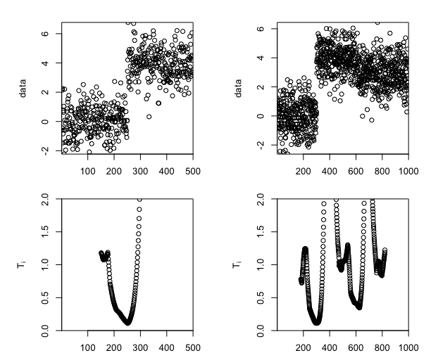
Figure 3: The upper two plots are for scatter points and the lower two plots are for the criterion functions $T_{n}(\cdot)$ for mean changes of normal distributions at the change points.

Table 1: Distribution of $\hat{K}-K$ with $K=11$ for various detection algorithms under CP model.

$\hat{K}-K$ Scenarios Procedures $\leq-3$ $-2$ -1 0 1 2 $\geq 3$ (i)$\sigma=1$ cumSeg 0 0 2 873 119 6 0 WBS 0 0 0 982 16 2 0 SMUCE 0 0 0 995 5 0 0 TMAR 0 0 0 998 2 0 0 (ii)$\sigma^{2}=3$ cumSeg 736 234 27 3 0 0 0 WBS 255 598 135 12 0 0 0 SMUCE 485 487 28 0 0 0 0 TMAR 0 2 46 645 264 39 4 (iii) cumSeg 21 707 236 30 6 0 0 WBS 0 422 457 119 2 0 0 SMUCE 0 342 488 170 0 0 0 TMAR 0 0 18 859 121 2 0 (iv) cumSeg 1000 0 0 0 0 0 0 WBS 0 0 0 0 1 5 993 SMUCE 0 0 0 0 0 0 1000 TMAR 1 8 66 331 384 164 46

Table 2: Distribution of $\hat{K}-K$ for various detection algorithms under CP alternative model.

$\hat{K}-K$ Scenarios Procedures $\leq-3$ $-2$ -1 0 1 2 $\geq 3$ (i)$\sigma=1$ cumSeg 237 262 251 150 94 6 0 WBS 7 49 215 599 128 2 0 SMUCE 18 128 535 318 1 0 0 TMAR 0 0 32 899 68 1 0 (ii)$\sigma^{2}=3$ cumSeg 1000 0 0 0 0 0 0 WBS 1000 0 0 0 0 0 0 SMUCE 1000 0 0 0 0 0 0 TMAR 2 15 92 262 314 210 105 (iii) cumSeg 999 1 0 0 0 0 0 WBS 997 3 0 0 0 0 0 SMUCE 1000 0 0 0 0 0 0 TMAR 1 8 90 466 320 95 20 (iv) cumSeg 997 3 0 0 0 0 0 WBS 0 0 0 1 1 6 992 SMUCE 0 0 0 0 0 0 1000 TMAR 0 8 72 553 297 66 4

Table 3: Distribution of $\hat{K}-K$ using various detection algorithms under CP model for variance change.

$\hat{K}-K$ Scenarios Procedures $\leq-3$ $-2$ -1 0 1 2 $\geq 3$ (i)$\sigma=1$ SMUCE 1000 0 0 0 0 0 0 BS 1000 0 0 0 0 0 0 PELT 17 2 0 981 0 0 0 TMAR 0 1 919 80 0 0 (ii)$\sigma^{2}=3$ SMUCE 1000 0 0 0 0 0 0 BS 1000 0 0 0 0 0 0 PELT 6 0 303 691 0 0 0 TMAR 0 0 96 903 1 0 0 (iii) SUMCE 1000 0 0 0 0 0 0 BS 1000 0 0 0 0 0 0 PELT 1000 0 0 0 0 0 0 TMAR 0 0 0 229 619 142 10 (iv) SMUCE 1000 0 0 0 0 0 0 BS 1000 0 0 0 0 0 0 PELT 2 5 2 79 69 173 670 TMAR 0 1 36 613 293 55 2