Iterate Averaging in the Quest for Best Test Error

Abstract

We analyse and explain the increased generalisation performance of iterate averaging using a Gaussian process perturbation model between the true and batch risk surface on the high dimensional quadratic. We derive three phenomena from our theoretical results: (1) The importance of combining iterate averaging (IA) with large learning rates and regularisation for improved regularisation. (2) Justification for less frequent averaging. (3) That we expect adaptive gradient methods to work equally well, or better, with iterate averaging than their non-adaptive counterparts. Inspired by these results, together with empirical investigations of the importance of appropriate regularisation for the solution diversity of the iterates, we propose two adaptive algorithms with iterate averaging. These give significantly better results compared to stochastic gradient descent (SGD), require less tuning and do not require early stopping or validation set monitoring. We showcase the efficacy of our approach on the CIFAR-10/100, ImageNet and Penn Treebank datasets on a variety of modern and classical network architectures.

Keywords: Iterate Averaging, Generalisation, Deep Learning Theory, Deep Learning Limit, Adaptive Gradient Methods

1 Introduction

Deep Neural Network (DNN) models achieve state of the art performance in a plethora of problems, such as speech recognition, visual object image recognition, object detection, drug discovery and genomics (LeCun et al., 2015). Of key interest is the ability of DNNs to “generalise” to unseen data, even when the parameter number greatly exceeds the dataset size (Zhang et al., 2016). DNNs are typically trained using stochastic gradient descent (SGD), in which model parameters at each optimisation step, ${\bm{w}}_{k+1}$, are updated using the gradient of the minibatch loss at the previous step, $L({\bm{w}}_{k})$:

$${\bm{w}}_{k+1}={\bm{w}}_{k}-\alpha_{k}\nabla L({\bm{w}}_{k}),$$ (1)

where $\alpha_{k}$ denotes the learning rate at iteration $k$. Whilst careful monitoring of the validation metrics, along with weight decay (Krogh and Hertz, 1992), layer-wise normalisation (Ioffe and Szegedy, 2015) and data-augmentation (Shorten and Khoshgoftaar, 2019; Zhang et al., 2017) help protect against over-fitting to the training data, the initial value of $\alpha_{k}$ and its schedule throughout training has a large impact on generalisation (Jastrzebski et al., 2017; Li et al., 2019), making it a key hyperparameter to set correctly. Theoretical results for optimal asymptotic training set convergence prescribe a learning rate proportional to the inverse square root of the number of iterations (Nesterov, 2013) or a decay at this rate (Duchi, 2018). However, such schedules often result in poor test set performance for DNNs. Curiously, Merity et al. (2017) and Izmailov et al. (2018) demonstrate that combining tail iterate averaging (i.e. taking an average of the last iterates in training) with large learning rate SGD increases DNN generalisation at the expense of training accuracy. However, quite why and how this works is still something of a mystery, limiting its widespread adoption.

One proposal in the literature to limit sensitivity to the learning rate and its schedule has been the development of adaptive gradient optimisers, which invoke a per-parameter learning rate based on the history of gradients. Popular examples include Adam (Kingma and Ba, 2014), AdaDelta (Zeiler, 2012) and RMSprop (Tieleman and Hinton, 2012). Ignoring momentum and explicit regularisation, the $k^{\mathrm{th}}$ iteration of a general adaptive optimiser is given by:

$${\bm{w}}_{k+1}\leftarrow{\bm{w}}_{k}-\alpha_{k}{\bm{B}}^{-1}\nabla L_{k}({\bm{w}}_{k}),$$ (2)

where the preconditioning matrix ${\bm{B}}$ typically approximates curvature information. Crucially, however, the generalisation of solutions found using adaptive methods, as measured in terms of test and validation error, significantly underperforms SGD (Wilson et al., 2017). Due to this, state-of-the-art convolutional neural networks, especially for image classification datasets such as CIFAR (Yun et al., 2019) and ImageNet (Xie et al., 2019; Cubuk et al., 2019) are still trained using SGD with momentum (Nesterov, 2013). Furthermore, despite Iterate Averaging (IA) being mentioned as a potential amendment in the original Adam paper (Kingma and Ba, 2014) and being required in the convergence proof (Reddi et al., 2019), it is not widely used for computer vision or other complex problems.

2 Contributions

The key contribution of this paper are:

• We investigate the impact of IA on generalisation by considering high-dimensional SGD on the quadratic model of the true risk perturbed by i.i.d. Gaussian noise, showing that the iterate average attains the global minimum, whereas the final point, despite multiple learning rate drops, or increases in batch size during training, does not.

• We extend the framework to a Gaussian process perturbation model between the true and batch gradients. We find that as long as certain technical conditions (well met in practice) are satisfied, the simplified result holds. Crucially, distance in weight space or relative weight space (depending on kernel choice) are pivotal to the effect, justifying in practice the need for large learning rates in conjunction with iterate averaging.

• We show that adaptive gradient methods have identical properties under the iterate average, but we expect them to converge faster than their non-adaptive counterparts.

• Motivated by these results, we consider why adaptive methods are not typically used in conjunction with iterate averaging? We find that ineffective regularisation, which limits the effective distance and prediction diversity between the iterates, is the main culprit and propose a simple, yet effective solution. We propose two Adam-based algorithms: Gadam and GadamX. Both outperform baselines tested for all networks and datasets we consider. GadamX achieves a Top-$1$ error of $22.69\%$ on ImageNet using ResNet-$50$, outperforming a well-tuned SGD baseline of $23.85\%$ (Chintala et al., 2017). To put this into perspective, the gain attributed to widely-adopted cosine schedules increases accuracy by $0.3\%$ (Bello et al., 2021).

• Showing that adaptive methods can outperform SGD and SGD with IA provides a practical framework that can be used, even for large-scale problems.

Related Work & Motivation:

To the best of our knowledge there has been no explicit theoretical work analysing the generalisation benefit of iterate averaging. Whilst Izmailov et al. (2018) propose that iterate averaging leads to “flatter minima which generalise better”, flatness metrics are known to have limitations as a proxy for generalisation (Dinh et al., 2017), in addition to which we show in the appendix Section E.1 that adaptive methods can find very sharp minima with good generalisation properties. Martens (2014) show that the IA convergence rate for both SGD and second-order methods are identical, but argue that second-order methods have an optimal pre-asymptotic convergence rate on a quadratic loss surface. Here, pre-asymptotic means before taking the number of iterations $t\rightarrow\infty$ and quadratic means that the Hessian is constant at all points in weight-space. The analysis does not extend to generalisation and no connection is made to adaptive gradient methods, nor to the importance of the high parameter-space dimensionality of the problem, two major contributions of our work. Amendments to improve the generalisation of adaptive methods include switching between Adam and SGD (Keskar and Socher, 2017) and decoupled weight decay (Loshchilov and Hutter, 2019), limiting the extent of adaptivity (Chen and Gu, 2018; Zhuang et al., 2020). We incorporate these insights into our algorithms but significantly outperform them experimentally. The closest algorithmic contribution to our work is Lookahead (Zhang et al., 2019b), which combines adaptive methods with an exponentially moving average scheme. We analyse this algorithm both theoretically (see appendix Section B) and experimentally.

3 Iterate Averaging: A New Theory for Generalisation

The iterate average (Polyak and Juditsky, 1992) is the arithmetic mean of the model parameters over the optimisation trajectory ${\bm{w}}_{\mathrm{avg}}=\frac{1}{n}\sum_{i}^{n}{\bm{w}}_{i}$. It is a classical variance reducing technique in optimisation and offers optimal asymptotic convergence rates and greater robustness to the choice of learning rate (Kushner and Yin, 2003). Indeed, popular regret bounds that form the basis of gradient-based convergence proofs (Duchi et al., 2011; Reddi et al., 2019) often consider convergence for the iterate average (Duchi, 2018). Further, theoretical extensions have shown that the rate of convergence can be improved by a factor of $\log T$ (where $T$ is the iteration number) by suffix averaging (Rakhlin et al., 2011), which considers a fraction of the last iterates, polynomial decay averaging (Shamir and Zhang, 2013) which decays the influence of the previous iterates, or weighted averaging (Lacoste-Julien et al., 2012) which weights the iterate by its iteration number. That the final iterate of SGD is sub-optimal in terms of its convergence rate, by this logarithmic factor, has been proved by Harvey et al. (2019). However, under an alternative decay schedule it can be shown to be equal to that of averaged schemes (Jain et al., 2019).

For networks with batch normalisation (Ioffe and Szegedy, 2015), a naïve application of IA (in which we simply average the batch normalisation statistics) is known to lead to poor results (Defazio and Bottou, 2019). However, by computing the batch normalisation statistics for the iterate average using a forward pass of the data at the IA point, Izmailov et al. (2018) show that the performance of small-scale image experiments such as CIFAR-10/100 and pretrained ImageNet can be significantly improved. Even for small experiments this computation is expensive, so they further approximate IA by taking the average at the end of each epoch instead of each iteration, referred to as stochastic weight averaging (SWA). We show experimentally in Section 10 that the two approaches produce almost identical results, with SWA slightly outperforming IA. Since SWA can be seen as IA with a lower averaging frequency, we retain the terminology IA - however, in our theoretical analysis we also include analysis for reduced frequency iterate averaging.

Notation:

• With some variable $n\rightarrow\infty$, and scalar-valued functions $f,g$, $f(n)=o(g(n))$ is shorthand for $f(n)/g(n)\rightarrow 0$ as $n\rightarrow\infty$. Similarly, $f(n)=\mathcal{O}(g(n))$ is shorthand for $f(n)/g(n)\rightarrow c$, for some constant $c>0$. In particular $\mathcal{O}(1)$ can be read as shorthand for any fixed non-zero constant, and $o(1)$ for any term which decays to $0$. For example $f(n)=3n+2+1/n$ can be abbreviated as $f(n)=\mathcal{O}(n)$, or $f(n)=3n+\mathcal{O}(1)$, or $f(n)=3n+2+o(1)$, depending on the the level of precision required. We will also employ the asymptotic equivalence notation $f(n)\sim g(n)$ to denote the special case $f(n)/g(n)\rightarrow 1$.

• For matrices $B$, $\|B\|_{F}=\sqrtsign{\sum_{ij}B_{ij}^{1/2}}$ denotes the Frobenius norm and $\|B\|=\sup_{\|q\|=1}\|B{\bm{q}}\|$ denotes the operator norm.

• For random vectors $X$, define $\|X\|_{\psi_{2}}=\inf\left\{t>0:\mathbb{E}\exp(X^{2}/t^{2})\leq 2\right\}$.

• For a set of $P$ positive eigenvalues $\lambda_{1},\ldots,\lambda_{P}$ and any rational function of $f$, $\langle f(\lambda)\rangle=\frac{1}{P}\sum_{i=1}^{P}f(\lambda_{i})$.

3.1 A High-Dimensional Geometry Perspective

We examine the variance reducing effect of IA in the context of a quadratic approximation to the true loss combined with additive perturbation models for the batch training loss.

The theory we present is high-dimensional (i.e. large number of parameters, $P$) and considers the small batch size (small $B$) regime, which we term the “deep learning limit”.

Intuitively, any given example from the training set $j\in\mathcal{D}$, will contain general features, which hold over the data generating distribution and instance specific features (which are relevant only to the training sample in question). For example, for a training image of a dog, we may have that:

$$\overbrace{\underbrace{\nabla L_{\text{sample}}({\bm{w}})}_{\textrm{training set example}}}^{\textrm{dog $j$}}=\overbrace{\underbrace{\nabla L_{\text{true}}({\bm{w}})}_{\textrm{general features}}}^{\textrm{$4$ legs, snout}}+\overbrace{\underbrace{{\bm{\epsilon}}({\bm{w}}).}_{\textrm{instance-specific features}}}^{\textrm{black pixel in top corner, green grass}}$$ (3)

Under a quadratic approximation to the true loss $L_{\text{true}}({\bm{w}})={\bm{w}}^{T}{\bm{H}}{\bm{w}}$, where ${\bm{H}}=\nabla^{2}L$ is the Hessian of the true loss with respect to the weights and we sample a mini-batch gradient of size $B$ at point ${\bm{w}}\in\mathbb{R}^{P\times 1}$. The observed gradient is perturbed by ${\bm{\epsilon}}({\bm{w}})$ from the true loss gradient (due to instance specific features). Under this model the component of the ${\bm{w}}_{t}$’th iterate along the $j$’th eigenvector ${\bm{\phi}}_{j}$ of the true loss when running SGD with learning rate $\alpha$ can be written:

$${\bm{w}}_{t}^{T}{\bm{\phi}}_{j}=(1-\alpha\lambda_{j})^{t}{\bm{w}}_{0}^{T}{\bm{\phi}}_{j}-\alpha(1-\alpha\lambda_{j})^{t-1}{\bm{\epsilon}}({\bm{w}}_{1})^{T}{\bm{\phi}}_{j}\cdots,$$ (4)

in which $\lambda_{j}$ are the eigenvalues of ${\bm{H}}$. The simplest tractable model for the gradient noise ${\bm{\epsilon}}({\bm{w}}_{t})$ is to assume samples from i.i.d. an isotropic, multivariate Normal. In particular, this assumption removes any dependence on ${\bm{w}}_{t}$ and precludes the existence of any distinguished directions in the gradient noise. Using this assumption, we obtain Theorem 2 below, which relies on an intermediate result, found in Vershynin (2018).

Lemma 1 (Vershynin (2018) Theorem 6.3.2)

Let $R$ be an $m\times n$ matrix, and let $X=(X_{1},\ldots,X_{n})\in\mathbb{R}^{n}$ be a random vector with independent mean-zero unit-variance sub-Gaussian coordinates. Then

$$\mathbb{P}\left(\left|\|RX\|_{2}-\|R\|_{F}\right|>t\right)\leq 2\exp\left(-\frac{ct^{2}}{K^{4}\|R\|^{2}}\right)$$

where $K=\max_{i}\|X_{i}\|_{\psi_{2}}$ and $c>0$ is a constant.

Theorem 2

Assume the aforementioned quadratic loss and i.i.d. Gaussian gradient noise model. Assume further that $\alpha\lambda_{i}\ll 1$ for all $i$ and $\lambda_{i}>0$ for all $i$. Then there exists a constant $c>0$ such that for all $t>0$, as $n\rightarrow\infty$

$$\mathbb{P}\left(\left|\sqrtsign{\sum_{i}^{P}\left(w_{n,i}-w_{0,i}\mathrm{e}^{-n\alpha\lambda_{i}}(1+o(1))\right)^{2}}-\sqrt{P\frac{\alpha\sigma^{2}}{B}\bigg{\langle}\frac{1}{\lambda(2-\alpha\lambda)}\bigg{\rangle}}\right|\geq t\right)\leq\nu(t),$$ (5)

$$\mathbb{P}\left(\left|\sqrtsign{\sum_{i}^{P}\left(w_{\mathrm{avg},i}-\frac{w_{0,i}}{\lambda_{i}n\alpha}(1+o(1))\right)^{2}}-\sqrt{\frac{P\sigma^{2}}{Bn}\bigg{\langle}\frac{1}{\lambda}\bigg{\rangle}}\right|\geq t\right)\leq\nu(t),$$

where $\nu(t)=2\exp(-ct^{2})$ and $B$ is the batch size.

Proof 

Let $Y=(Y_{1},\ldots,Y_{P})$ be a random sub-Gaussian vector with independent components. Let

$$X_{i}=\frac{Y_{i}-\mathbb{E}Y_{i}}{\sqrtsign{\mathrm{Var}Y_{i}}},~{}~{}R=\mathrm{diag}(\sqrtsign{\mathrm{Var}Y_{1}},\ldots,\sqrtsign{\mathrm{Var}Y_{P}}).$$

Lemma 1 then applies, to give

$$\mathbb{P}\left(\left|\|Y-\mathbb{E}Y\|_{2}-\sqrtsign{\sum_{i=1}^{P}\mathrm{Var}Y_{i}}\right|>t\right)\leq 2\exp\left(-\frac{ct^{2}}{K^{4}\|R\|^{2}}\right).$$

We have $K\leq C\max_{i}\mathrm{Var}Y_{i}$ for some constant $C>0$ (Vershynin (2018), exercise 2.5.8), and $\|R\|^{2}=(\max_{i}\sqrtsign{\mathrm{Var}Y_{i}})^{2}=\max_{i}\mathrm{Var}Y_{i}$. Hence we obtain

$$\mathbb{P}\left(\left|\|Y-\mathbb{E}Y\|_{2}-\sqrtsign{\sum_{i=1}^{P}\mathrm{Var}Y_{i}}\right|>t\right)\leq 2\exp\left(-\frac{ct^{2}}{(\max_{i}\mathrm{Var}Y_{i})^{2}}\right)$$ (6)

for some new constant $c>0$. The proof is then completed if we compute the means and variances of ${\bm{w}}_{n}$ and ${\bm{w}}_{\mathrm{avg}}$. To that end, with ${\bm{\Lambda}}=\text{diag}\left(\lambda_{1},\ldots,\lambda_{P}\right)$, we have

$${\bm{w}}_{n}=(1-\alpha{\bm{\Lambda}})^{n}{\bm{w}}_{0}+\alpha\sum_{i=0}^{n-1}(1-\alpha{\bm{\Lambda}})^{n-i-1}{\bm{\epsilon}}_{i}.$$ (7)

Summation then gives

$${\bm{w}}_{avg} =\frac{1-(1-\alpha{\bm{\Lambda}})^{n}}{\alpha n}{\bm{\Lambda}}^{-1}(1-\alpha{\bm{\Lambda}}){\bm{w}}_{0}+\sum_{i=0}^{n-1}\frac{1-(1-\alpha{\bm{\Lambda}})^{n-i}}{n}{\bm{\Lambda}}^{-1}{\bm{\epsilon}}_{i}.$$ (8)

With all the ${\bm{\epsilon}}_{i}$ being i.i.d. $\mathcal{N}(0,\sigma^{2}B^{-1}I)$, we need simply to compute the sums

$$\sum_{i=1}^{n-1}\alpha^{2}(1-\alpha{\bm{\Lambda}})^{2(n-i-1)} =\alpha^{2}(1-(1-\alpha{\bm{\Lambda}})^{2n})\left(1-(1-\alpha{\bm{\Lambda}})^{2}\right)^{-1}$$ (9)

and similarly

$$\sum_{i=0}^{n-1}\left(\frac{1-(1-\alpha{\bm{\Lambda}})^{n-i}}{n}{\bm{\Lambda}}^{-1}\right)^{2}$$ (10)

$$= \frac{{\bm{\Lambda}}^{-2}}{n^{2}}\left(n-\frac{2(1-(1-\alpha{\bm{\Lambda}})^{n})}{\alpha}{\bm{\Lambda}}^{-1}+\left(1-(1-\alpha{\bm{\Lambda}})^{2n}\right)\left(1-(1-\alpha{\bm{\Lambda}})^{2}\right)^{-1}\right).$$ (11)

Now assuming $\alpha\lambda_{i}\ll 1$ for all $i=1,2\ldots,P$, and taking $n\rightarrow\infty$, we find

$$\sum_{i=1}^{n-1}(1-\alpha{\bm{\Lambda}})^{2(n-i-1)}\sim\alpha^{2}\left(1-(1-\alpha{\bm{\Lambda}})^{2}\right)^{-1}=\alpha\left(2{\bm{\Lambda}}-\alpha{\bm{\Lambda}}^{2}\right)^{-1}$$ (12)

and similarly

$$\sum_{i=0}^{n-1}\left(\frac{1-(1-\alpha{\bm{\Lambda}})^{n-i}}{n}{\bm{\Lambda}}^{-1}\right)^{2}\sim\frac{1}{n}{\bm{\Lambda}}^{-2}.$$ (13)

Thus it follows that

$$\mathbb{E}w_{n,i}=(1-\alpha\lambda_{i})^{n}w_{0,i}\sim e^{-2\alpha\lambda_{i}}w_{0,i}, ~{}~{}\mathrm{Var}(w_{n,i})\sim\frac{\sigma^{2}}{B}\frac{\alpha}{2\lambda_{i}(1-\alpha\lambda_{i})}$$ (14)

and

$$\mathbb{E}w_{avg,i}\sim\frac{w_{0,i}}{\lambda_{i}\alpha n},~{}~{}~{}\mathrm{Var}(w_{avg,i})=\frac{\sigma^{2}}{B}\frac{1}{n\lambda_{i}^{2}}$$ (15)

where in both cases we have used $\alpha\lambda_{i}\ll 1$. The proof is now completed by applying (6) and noting that $\max_{i}\mathrm{Var}(w_{n,i})$ and $\max_{i}\mathrm{Var}(w_{\mathrm{avg}),i}$ are finite so long as $\alpha\lambda_{i}\ll 1$ for all $i$ and $\lambda_{i}>0$ for all $i$ (as we have already assumed).  
The final iterate attains exponential convergence in the mean of ${\bm{w}}_{n}$, but does not control the variance term. Whereas for ${\bm{w}}_{\mathrm{avg}}$, although the convergence in the mean is worse (linear), the variance vanishes asymptotically – this motivates tail averaging, to get the best of both worlds. Another key implication of Theorem 2 lies in its dependence on $P$. With $P$ being a rough gauge of the model complexity, the result implies that in more complex, over-parameterised models, we expect the benefit of IA over the final iterate to be larger due to the corresponding variance reduction. We show this explicitly in our experiments in Figure 4(c). Note the limited extra improvement possible by simply increasing the batch size, compared to IA asymptotically.

3.2 A dependent model for the perturbation

We proceed now to propose a relaxation of the gradient perturbation independence assumption. (3) can be written equivalently as

$$L_{\text{batch}}({\bm{w}})=L_{\text{true}}({\bm{w}})+\eta({\bm{w}})$$ (16)

where $\eta$ is a scalar field with $\nabla\eta={\bm{\epsilon}}$. Note that we have neglected an irrelevant arbitrary constant in Equation (16) and also that we have $L_{\text{batch}}$ rather than $L_{\text{sample}}$, but this amounts to scaling the per-sample noise variance $\sigma^{2}$ by the inverse batch size $B^{-1}$. We model $\eta$ as a Gaussian process $\mathcal{GP}(m,k)$, where $k$ is some kernel function $\mathbb{R}^{P}\times\mathbb{R}^{P}\rightarrow\mathbb{R}$ and $m$ is some mean function $\mathbb{R}^{P}\rightarrow\mathbb{R}$. As an example, taking $k({\bm{w}},{\bm{w}}^{\prime})\propto({\bm{w}}^{T}{\bm{w}}^{\prime})^{p}$ and restricting ${\bm{w}}$ to a hypersphere results in ${\bm{\epsilon}}$ taking the exact form of a spherical $p$-spin glass, studied previously for DNNs (Choromanska et al., 2015; Gardner and Derrida, 1988; Mezard et al., 1987; Ros et al., 2019; Mannelli et al., 2019; Baskerville et al., 2021a, b). We are not proposing to model the loss surface (batch or true) as a spin glass (or more generally, a Gaussian process), rather we are modelling the perturbation between the loss surfaces in this way. We emphasise that this model is a strict generalisation of the i.i.d. assumption above, and presents a rich, but tractable, model of isotropic Gaussian gradient perturbations in which the noise for different iterates is neither independent nor identically distributed.

Following from our Gaussian process definition, the covariance of gradient perturbations can be computed using a well-known result (see Adler and Taylor (2009) equation 5.5.4):

$$\mathrm{Cov}(\epsilon_{i}({\bm{w}}),\epsilon_{j}({\bm{w}}^{\prime}))=\partial_{w_{i}}\partial_{w^{\prime}_{j}}k({\bm{w}},{\bm{w}}^{\prime}).$$ (17)

Further assuming a stationary kernel $k({\bm{w}},{\bm{w}}^{\prime})=k\left(-\frac{1}{2}||{\bm{w}}-{\bm{w}}^{\prime}||_{2}^{2}\right)$

$$\mathrm{Cov}(\epsilon_{i}({\bm{w}}),\epsilon_{j}({\bm{w}}^{\prime}))=(w_{i}-w^{\prime}_{i})(w^{\prime}_{j}-w_{j})k^{\prime\prime}\left(-\frac{1}{2}||{\bm{w}}-{\bm{w}}^{\prime}||_{2}^{2}\right)+\delta_{ij}k^{\prime}\left(-\frac{1}{2}||{\bm{w}}-{\bm{w}}^{\prime}||_{2}^{2}\right).$$ (18)

Thus we have a non-trivial covariance between gradient perturbation at different points in weight-space. This covariance structure can be used to prove the upcoming variance reduction result. Its proof relies on some technical Lemmas (proved in the appendix, Section A.1) which we now state.

Lemma 3

Let ${\bm{X}}_{1},\ldots,{\bm{X}}_{n}$ be a sequence of multivariate Gaussian random variables in $\mathbb{R}^{P}$ with

$${\bm{X}}_{i}\mid\{{\bm{X}}_{j}\mid 0<j<i\}\sim\mathcal{N}(0,\sigma^{2}I)$$

for all $1\leq i\leq n$. Let ${\bm{X}}_{0}$ be any deterministic element of $\mathbb{R}^{P}.$ Define the events

$$A_{m}(\delta)=\{||{\bm{X}}_{i}-{\bm{X}}_{j}||_{2}>\delta\mid 0\leq i<j\leq n\}.$$

Consider $P\rightarrow\infty$ with $P\gg\log{n}$ and let $\delta>0$ be $o(P^{\frac{1}{2}})$ (note that $\delta$ and $n$ need not diverge with $P$, but they can). Then $\mathbb{P}(A_{n}(\delta))\rightarrow 1$ as $P\rightarrow\infty$.

Lemma 4

Assume the covariance structure (18). Take any $a_{i}\in\mathbb{R}$ and define $\bar{{\bm{\epsilon}}}=\sum_{i=1}^{n}a_{i}{\bm{\epsilon}}_{i}$. Then

$$\operatorname{Tr}~{}\mathrm{Cov}(\bar{{\bm{\epsilon}}}) =k^{\prime}(0)P\sum_{i=1}^{n}a_{i}^{2}+2P\sum_{1\leq i<j\leq n}a_{i}a_{j}\Bigg{[}k^{\prime}(-\frac{d_{ij}^{2}}{2})+P^{-1}k^{\prime\prime}(-\frac{d_{ij}^{2}}{2})d_{ij}^{2}\Bigg{]}$$ (19)

where we define $d_{ij}=||{\bm{w}}_{i}-{\bm{w}}_{j}||_{2}$.

Theorem 5

Let ${\bm{w}}_{n}$ and ${\bm{w}}_{avg}$ be defined as in Theorem 2 and let the gradient perturbation be given by the covariance structure in (17). Assume that the kernel function $k$ is such that $k^{\prime}(-x^{2})$ and $x^{2}k^{\prime\prime}(-x^{2})$ decay as $x\rightarrow\infty$, and define $\sigma^{2}B^{-1}=k^{\prime}(0)$. Assume further that $P\gg\log n$. Let $\delta=o(P^{1/2})$. Then ${\bm{w}}_{n}$ and ${\bm{w}}_{avg}$ are multivariate Gaussian random variables and, with probability which approaches unity as $P,n\rightarrow\infty$ the iterates ${\bm{w}}_{t}$ are all mutually at least $\delta$ apart and

$$\mathbb{E}w_{n,i}\sim e^{-\alpha\lambda_{i}n}w_{0,i}, \frac{1}{P}\operatorname{Tr}\mathrm{Cov}({\bm{w}}_{n})\sim\frac{\alpha\sigma^{2}}{B}\left\langle\frac{1}{\lambda(2-\alpha\lambda)}\right\rangle,$$ (20)

$$\mathbb{E}w_{avg,i}\sim\frac{1-\alpha\lambda_{i}}{\alpha\lambda_{i}n}w_{0,i}, \frac{1}{P}\operatorname{Tr}\mathrm{Cov}({\bm{w}}_{avg})\leq\frac{\sigma^{2}}{Bn}\left\langle\frac{1}{\lambda}\right\rangle+\mathcal{O}(1)\Bigg{(}k^{\prime}(-\frac{\delta^{2}}{2})+P^{-1}\delta^{2}k^{\prime\prime}(-\frac{\delta^{2}}{2})\Bigg{)}.$$ (21)

Proof  We will prove the result in the case $\lambda_{i}=\lambda~{}\forall i$ for the sake of clarity. The same reasoning can be repeated in the more general case; where one gets $P^{-1}f(\lambda)\operatorname{Tr}I$ below, one need only replace it with $\langle f(\lambda)\rangle$, exploiting linearity of the trace. We will also vacuously replace $\sigma^{2}B^{-1}$ with $\sigma^{2}$ to save on notation. For weight iterates ${\bm{w}}_{i}$, we have the recurrence

$${\bm{w}}_{i}=(1-\alpha\lambda){\bm{w}}_{i-1}+\alpha{\bm{\epsilon}}({\bm{w}}_{i-1})$$

which leads to

$${\bm{w}}_{n}=(1-\alpha\lambda)^{n}{\bm{w}}_{0}+\alpha\sum_{i=0}^{n-1}(1-\alpha\lambda_{i})^{n-i-1}{\bm{\epsilon}}({\bm{w}}_{i})$$ (22)

and then

$${\bm{w}}_{avg} =\frac{1-(1-\alpha\lambda)^{n}}{\alpha\lambda n}(1-\alpha\lambda){\bm{w}}_{0}+\sum_{i=0}^{n-1}{\bm{\epsilon}}({\bm{w}}_{i})\frac{1-(1-\alpha\lambda)^{n-i}}{\lambda n}.$$ (23)

Now define

$$a_{i}=\alpha(1-\alpha\lambda)^{n-1-i},~{}~{}~{}\bar{a}_{i}=\frac{1-(1-\alpha\lambda)^{n-i}}{\lambda n}.$$

Next we will apply Lemma 4 and utilise Lemma 3 to bound the variance of ${\bm{w}}_{avg}$ and ${\bm{w}}_{n}$. We first gather the following facts (which were also computed and used in the proof of Theorem $1$:

$$\sum_{i=1}^{n-1}a_{i}^{2} =\frac{\alpha^{2}(1-(1-\alpha\lambda)^{2n})}{1-(1-\alpha\lambda)^{2}}$$ (24)

$$\sum_{i<j}a_{i}a_{j} =\frac{\alpha}{\lambda}\left(\frac{1-(1-\alpha\lambda)^{n}}{\alpha\lambda}-\frac{1-(1-\alpha\lambda)^{2n}}{1-(1-\alpha\lambda)^{2}}\right).$$ (25)

The sum of squares for the $\bar{a}_{i}$ is simple to obtain similarly

$$\sum_{i=0}^{n-1}\bar{a}_{i}^{2}=\frac{1}{\lambda^{2}n^{2}}\left(n-\frac{2(1-(1-\alpha\lambda)^{n})}{\alpha\lambda}+\frac{1-(1-\alpha\lambda)^{2n}}{1-(1-\alpha\lambda)^{2}}\right).$$ (26)

We now use the assumption that $0<\alpha\lambda<1$ (required for the convergence of gradient descent) which gives, as $n\rightarrow\infty$,

$$\sum_{i=1}^{n-1}a_{i}^{2} \sim\frac{\alpha^{2}}{1-(1-\alpha\lambda)^{2}}$$ (27)

$$\sum_{i<j}a_{i}a_{j} \sim\frac{\alpha}{\lambda}\left(\frac{1}{\alpha\lambda}-\frac{1}{1-(1-\alpha\lambda)^{2}}\right)$$ (28)

$$\sum_{i=1}^{n-1}\bar{a}_{i}^{2} \sim\frac{1}{\lambda^{2}n}$$ (29)

Summing $\sum_{i<j}\bar{a}_{i}\bar{a}_{j}$ explicitly is possible but unhelpfully complicated. Instead, some elementary bounds give

$$\sum_{i<j}\bar{a}_{i}\bar{a}_{j} \leq\left(\sum_{i=0}^{n-1}\bar{a}_{i}\right)^{2}=\frac{1}{\lambda^{2}n^{2}}\left(n-\frac{1-(1-\alpha\lambda)^{n}}{\alpha\lambda}\right)^{2}\sim\frac{1}{\lambda^{2}}$$

and

$$\sum_{i<j}\bar{a}_{i}\bar{a}_{j} \geq\sum_{i<j}\left(\frac{1-(1-\alpha\lambda)^{n-1}}{\lambda n}\right)^{2}\sim\frac{1}{2\lambda^{2}}$$

so in particular $\sum_{i<j}\bar{a}_{i}\bar{a}_{j}=\mathcal{O}(1)$. Now define the events $A_{n}(\delta)$ as in Lemma 3 using ${\bm{\epsilon}}_{i}$ in place of ${\bm{X}}_{i}$. Further, choose $\delta$ large enough so that $k^{\prime}(-\frac{x^{2}}{2})$ and $x^{2}k^{\prime\prime}(-\frac{x^{2}}{2})$ are decreasing for $x>\delta$. Define $k^{\prime}(0)=\sigma^{2}$. Lemma 4 gives

$$\frac{1}{P}\operatorname{Tr}\mathrm{Cov}({\bm{w}}_{n})\mid A_{n}(\delta) \leq\sigma^{2}\sum_{i=1}^{n}a_{i}^{2}+2\sum_{i<j}a_{i}a_{j}\Bigg{(}k^{\prime}(-\frac{\delta^{2}}{2})+P^{-1}\delta^{2}k^{\prime\prime}(-\frac{\delta^{2}}{2})\Bigg{)}$$ (30)

where we note that we have only upper-bounded the second term in (30), so using (27) and (28) and taking $\delta$ large enough we obtain

$$\frac{1}{P}\operatorname{Tr}\mathrm{Cov}({\bm{w}}_{n})\mid A_{n}(\delta)=\frac{\sigma^{2}\alpha^{2}}{1-(1-\alpha\lambda)^{2}}+o(1).$$ (31)

Turning now to ${\bm{w}}_{avg}$ we similarly obtain

$$\frac{1}{P}\operatorname{Tr}\mathrm{Cov}({\bm{w}}_{avg})\mid A_{n}(\delta)\leq\frac{\sigma^{2}}{n}\frac{1}{\lambda^{2}}+\mathcal{O}(1)\Bigg{(}k^{\prime}(-\frac{\delta^{2}}{2})+P^{-1}\delta^{2}k^{\prime\prime}(-\frac{\delta^{2}}{2})\Bigg{)}$$ (32)

and, as before, taking $\delta$ large enough we can obtain

$$\frac{1}{P}\operatorname{Tr}\mathrm{Cov}({\bm{w}}_{avg})\mid A_{n}(\delta)=o(1).$$ (33)

Finally recalling (22) and (23) and writing $(1-\alpha\lambda)^{n}=\text{e}^{-\alpha\lambda n}+o(1)$ for large $n$, we obtain the result.  

Note that Theorem 5 is a generalisation of Theorem 2 to the context of our dependent perturbation model. Let us make some clarifying remarks about the theorem and its proof:

1. The bound (21) in the statement of the theorem relies on all iterates being separated by a distance at least $\delta$. Moreover, the bound is only useful if $\delta$ is large enough to ensure the $k^{\prime}$ and $k^{\prime\prime}$ terms are small.

2. Just as in the independent case of Theorem 2, the first term in the bound in (21) decays only in the case that the number of iterates $n\rightarrow\infty$.

3. The remaining conditions on $P,n,\delta$ are required for the high-dimensional probability argument which we use to ensure that all iterates are separated by at least $\delta$.

4. $P\gg\log{n}$ is a perfectly reasonable condition in the context of deep learning. E.g. for a ResNet-50 with $P\approx 25\times 10^{6}$, violation of this condition would require $n>10^{10^{7}}$. A typical ResNet schedule on ImageNet has $<10^{6}$ total steps.

Consequently, our result points to the importance of good separation between weight iterates in IA to retain the independence benefit and variance reduction in a non-independent noise setting, hence one would expect large learning rates to play a crucial role in successful IA. At the same time, our result is particularly adapted to the deep learning limit of very many model parameters ($P\rightarrow\infty$), since this is the only regime in which we can argue probabilistically for good separation of weight iterates (otherwise one may simply have to assume such separation). Furthermore, the importance of $P\gg\log n$ indicates that perhaps averaging less frequently than every iteration could be beneficial to generalisation. The following corollary makes this intuition precise.

Corollary 6

Let ${\bm{w}}_{avg}$ now be a strided iterate average with stride $\kappa$, i.e.

$${\bm{w}}_{avg}=\frac{\kappa}{n}\sum_{i=1}^{\lfloor n/\kappa\rfloor}{\bm{w}}_{i}.$$ (34)

Then, under the same conditions as Theorem 5

$$\mathbb{E}w_{avg,i}=\frac{\kappa(1-\alpha\lambda_{i})^{\kappa}}{n(1-(1-\alpha\lambda_{i})^{\kappa})}(1+o(1))w_{0,i},$$ (35)

$$\frac{1}{P}\operatorname{Tr}\mathrm{Cov}({\bm{w}}_{avg})\leq\frac{\sigma^{2}\alpha^{2}\kappa}{Bn}\left\langle\frac{1}{\left(1-(1-\alpha\lambda)^{\kappa}\right)^{2}}\frac{1-(1-\alpha\lambda)^{2\kappa}}{1-(1-\alpha\lambda)^{2}}\right\rangle+\mathcal{O}(1)\Bigg{(}k^{\prime}(-\frac{\delta^{2}}{2})+P^{-1}\delta^{2}k^{\prime\prime}(-\frac{\delta^{2}}{2})\Bigg{)}$$ (36)

where the constant $\mathcal{O}(1)$ coefficient of the second term in (36) is independent of $\kappa$.

Proof  Very similar to that of Theorem 5. See appendix Section A.2.  

Intuitively, the first term in the covariance in (21) is an “independence term”, i.e. it is common between Theorems 2 and 5 and represents the simple variance reducing effect of averaging. The second variance term in (21) comes from dependence between the iterate gradient perturbations. We see from the corollary that an independent model for gradient perturbation would predict an unambiguous inflationary effect of strided IA on variance (the first term in (36)). However introducing dependence in the manner that we have predicts a more nuanced picture, where increased distance between weight iterates can counteract the simple “independent term” inflationary effect of striding, leaving open the possibility for striding to improve on standard IA for the purposes of generalisation. We investigate and experimentally confirm this hypothesis in Section 9.

3.3 Validation of Theory:

To better understand the effect of the large learning learning rate on generalisation, we train a VGG-$16$ network (Simonyan and Zisserman, 2014) with no data augmentation/batch normalisation (to isolate the overfitting effect from reducing the learning rate) with a learning rate of $\alpha=0.05$. Replacing the learning rate drop (performed at epoch $60$ by a factor of $10$ with weight decay $\gamma=0.0005$) with IA at the same point, we find that the test error is reduced by a greater margin ($\approx 2\%$), shown in Figure 1(a). We note that IA improves over the SGD learning rate equivalent for all values of weight decay, with results for $10$ seeds shown in Fig 1(b) and hence this argument is independent of explicit regularisation as indicated by Theorem 5. For our Deep Neural Network experiments, we find that the best IA optimiser improvement over its base optimiser is proportional to the number of parameters $P$ as shown in Fig 4(c) and predicted by Theorem 2. This theorem and experimental validation thereof translates into the following advice for practitioners: In the deep learning limit (large $P$ and small relative $B$) one should keep the learning rate high and use iterate averaging instead of sharply dropping the learning rate!

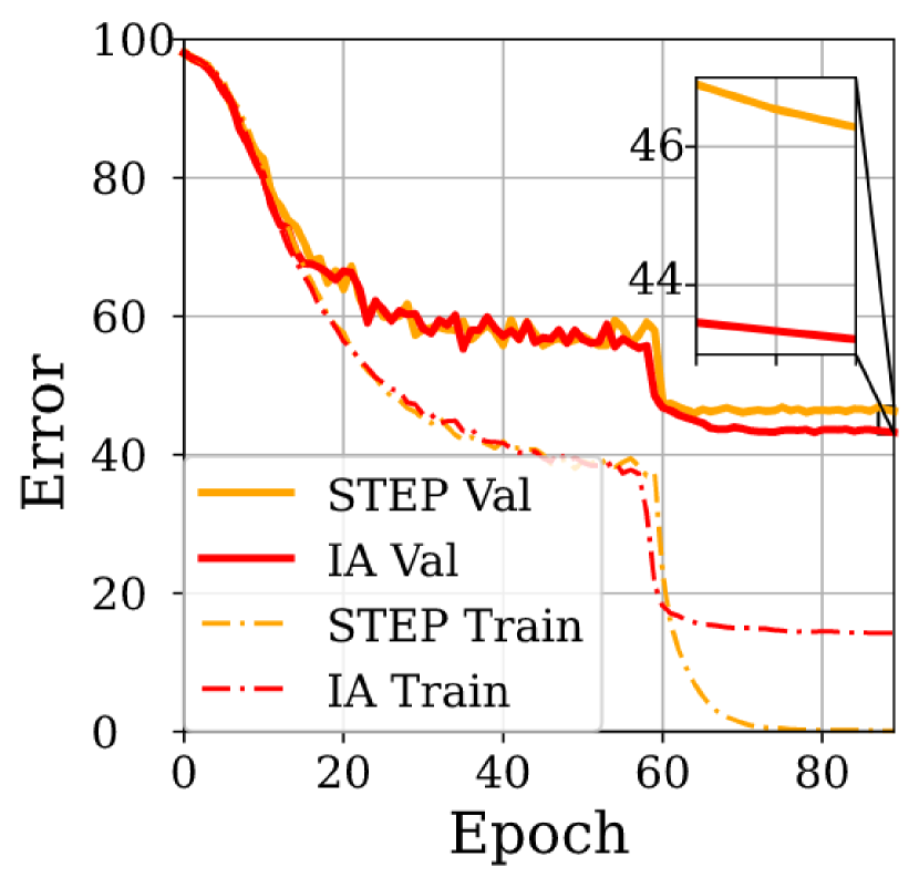
(a) IA vs STEP schedule

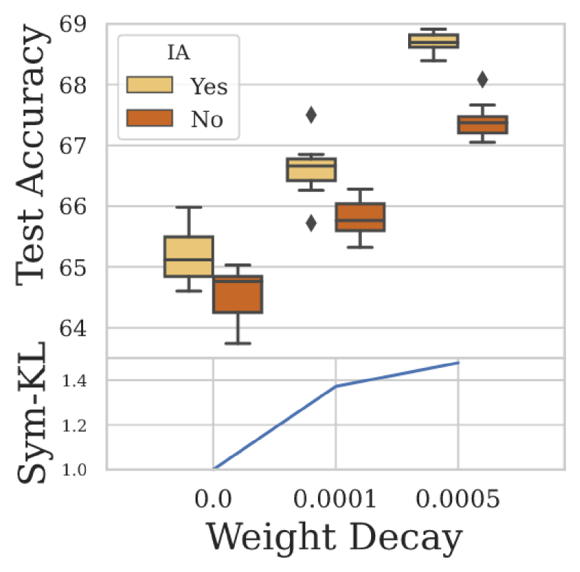
(b) Weight Decay Impact

Figure 1: (a) STEP (learning rate decay) and IA Train/Val error. Both approaches reduce Val error, but IA by a greater margin. (b) Effect of weight decay on held out test error for IA/sharp learning rate decay solutions. Greater weight decay increases the margin of IA improvement. The lower subplot shows the average symmetric KL-divergence between IA solutions.

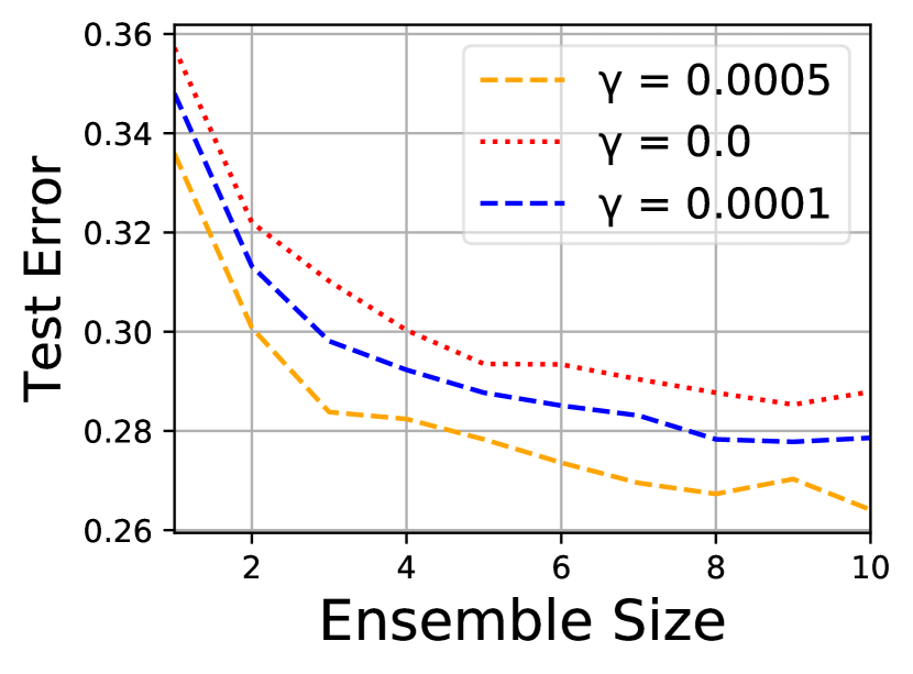
(a) Network Ensemble

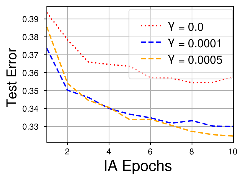
(b) Iterate Averaging

Figure 2: Test error improvement with differing degrees of regularisation $\gamma$ for (a) network ensembling and (b) IA.

3.4 A Closer Look at IA and the Importance of Regularisation

Izmailov et al. (2018) argue, under a linearisation assumption, that IA can be seen as approximate model ensembling. Since averaging only improves test performance for sufficiently uncorrelated models (through a reduction in variance of the ensemble), we must ensure sufficiently diverse models at each epoch through our training procedure. We note from Fig 2(b), that unlike model ensembling (shown in Fig 2(a)), the IA improvement is strongly dependent on the use of weight decay. We show the difference between IA and sharply decaying learning rate schedules (which mirror conventional setups) over $10$ seeds as a function of weight decay coefficient in Fig 1(b). The margin of improvement from IA, over sharply decaying schedules, steadily increases with regularisation - with $\gamma=0.0005$ (where $\gamma$ denotes the amount of weight decay or the coefficient of $L_{2}$ regularisation in the loss) delivering a greater final validation accuracy at the final IA point, despite starting from a lower accuracy compared to $\gamma=0.0001$. To explicitly show that such weight decay regularisation encourages greater diversity in the iterates we calculate the symmetrised KL-divergence, $\frac{1}{2}(\sum p(x)\log\frac{p(x)}{q(x)}+q(x)\log\frac{q(x)}{p(x)})$, over the entire test set between the softmax outputs of the IA iterates. We take an average for each weight decay value (normalising the $0$ weight decay value to $1$), as shown in the lower subfigure of Fig 1(b). As expected, greater weight decay gives greater solution diversity.

Distance in weight space or relative distance?

Theorem 5 relies on sufficiently large distances in weight-space between iterates to achieve variance reduction with IA. It is therefore natural to ask if weight decay encourages greater separation between iterates and if this separation in turn explains the efficacy of weight decay. For learning rate $\alpha$ and weight decay $\gamma$, we move a distance $\alpha\nabla L({\bm{w}})-\alpha\gamma{\bm{w}}$ in weight space. Intuitively, since random vectors in high dimensions are nearly orthogonal with high probability (Vershynin, 2018), we expect the distance in weight space to move a distance $\alpha\sqrt{(\nabla L({\bm{w}}))^{2}+\gamma^{2}{\bm{w}}^{2}}$, which is larger for $\gamma>0$. Conversely, we expect $||{\bm{w}}||^{2}$ to be smaller for smaller $\gamma$ and the gradients also to be smaller (Granziol, 2020). For the experiment (with equal learning rates) shown in Fig 1(b), the average distances between the IA epochs for weight decay values $\gamma=\{0,0.0001,0.0005\}$ are $17.7,14.9,13.9$, respectively. We note, however, that the relative distance, when normalised by the average weight norm, increases successively as $0.11,0.13,0.22$. This begs the question whether Theorem 5 can be extended to include a notion of relative distance.

Theorem 7

Let ${\bm{w}}_{n}$ and ${\bm{w}}_{avg}$ be defined as in Theorem 5 and let the gradient noise be given by the basic covariance structure in (17). Let the kernel function be of the form

$$k({\bm{w}},{\bm{w}}^{\prime})=k\left(-\frac{\|{\bm{w}}-{\bm{w}}^{\prime}\|_{2}^{2}}{\|{\bm{w}}\|_{2}\|{\bm{w}}^{\prime}\|_{2}}\right)$$

and assume that the kernel function $k$ is such that $k^{\prime}(-x^{2})$ and $x^{2}k^{\prime\prime}(-x^{2})$ decay as $x\rightarrow\infty$, and define $\sigma^{2}B^{-1}=k^{\prime}(0)$. Assume further that $P\gg\log n$. Then the result of Theorem 5 holds.

Proof  A minor modification of the proof of Theorem 5 and so is relegated to the appendix Section A.2.  

In Theorem 5 it is the absolute distance between iterates that determines the strength of dependence. In Theorem 7, the gradient noise covariance is sensitive instead to the the relative distance. This notion can be easily extended to products of weights in different layers, which is known to be invariant with the use of batch normalisation (Ioffe and Szegedy, 2015), used in many modern networks.

4 Adaptive Gradient Methods with Iterate Averaging

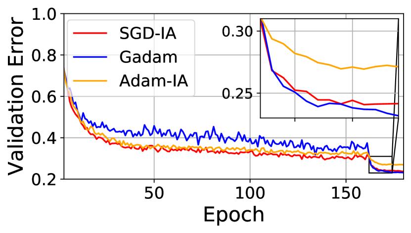
(a) Prn-$110$ Val. Error

Optim	SGD-IA	Adam-IA	Gadam
$\mathcal{D}(p||q)$	20.2	19.1	22.8
$||p-q||^{2}$	18.2	18.0	18.6
$\Delta E$	9.0	5.8	11.9
Values except $\Delta E$ in units of $1000$.

(b) Solution diversity

Figure 3: (a) Validation error for the PreResNet-$110$ on CIFAR-$100$ for various optimisers using IA and (b) the solution diversity given as the symmetrised KL $\mathcal{D}$ or total variation distance calculated on the test set and the change in validation error $\Delta E$ for the final IA point.

(a) Val Error

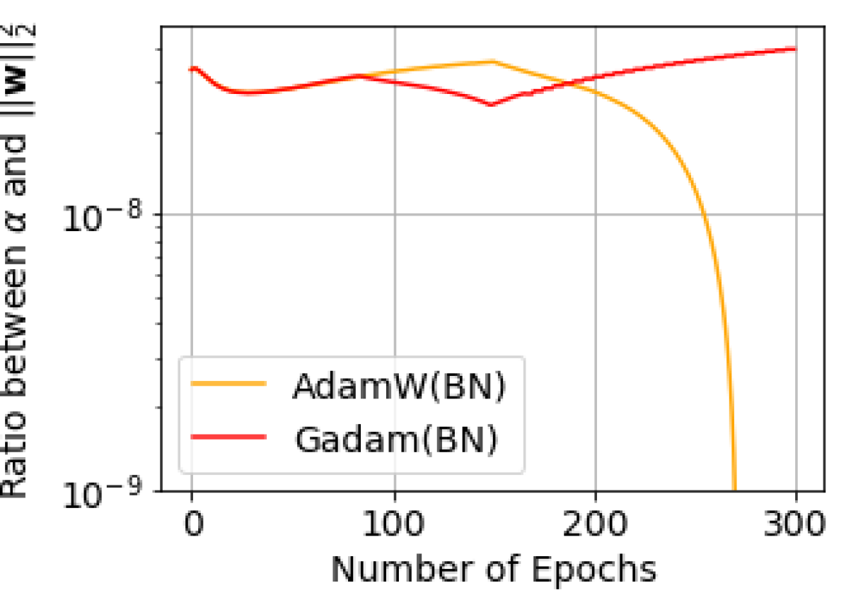
(b) ${\alpha}/{||{\bm{w}}||^{2}}$

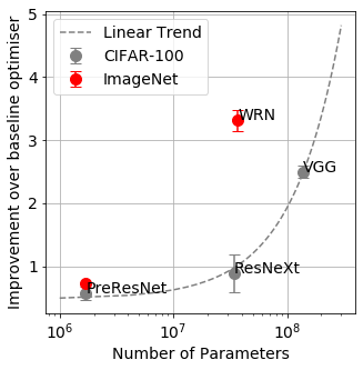
(c) Improvement vs. $P$

Figure 4: (a) Val. error and (b) effective learning rate $\frac{\alpha}{||{\bm{w}}||^{2}}$ of VGG-16 on CIFAR-100 with and without BN. (c) Improvement in using IA over the base optimiser for a variety of networks, closely following the linear trend.

Naïvely combining IA with Adam is not effective, as shown in Figure 3(a). Despite the same $L_{2}$ regularisation ($0.0001$), the error drop is significantly less than for SGD-IA. Following our intuition from Sec 3.4, we consider whether the problem could be that overly correlated solutions form the IA due to ineffective regularisation. As shown in Tab. (b) of Figure 3, both the symmetrised KL divergence $\mathcal{D}(p||q)$ and total variation distance $||p-q||^{2}$ (calculated between all epochs using IA at the end of training and then averaged) are lower for Adam-IA than for SGD-IA. For adaptive optimisers, $L_{2}$ regularisation is not equivalent to weight decay (Zhang et al., 2018; Loshchilov and Hutter, 2019), with weight decay generalising better - known as AdamW. For AdamW with a decoupled weight decay of $0.25$, the solution diversity increases beyond that of SGD-IA. This is accompanied by a greater drop in validation error, even outperforming SGD-IA. We term this combination of AdamW + IA Gadam to denote a variant of Adam that generalises. Previous work has shown that limiting the belief in the Adam curvature matrix improves generalisation (Zhuang et al., 2020; Chen and Gu, 2018), hence we also incorporate such a partially adaptive Adam into our framework and term the resulting Algorithm GadamX.

For convolutional neural networks using batch normalisation, the effective learning rate is proportional to $\alpha_{\mathrm{eff}}\propto\frac{\alpha}{||{\bm{w}}||^{2}}$ (Hoffer et al., 2018). With batch normalisation, the output is invariant to the channel weight norm, hence weight changes are only with respect to the direction of the vector. Since the effective weight decay depends on the (effective) learning rate, we expect this to lead to more regularised solutions and better validation error. To test this hypothesis, we train a VGG-16 network on CIFAR-100 with and without BN (see Figs 4(a),4(b)): for an identical setup, the margin of improvement of Gadam over AdamW is much larger with BN. We note that while Gadam keeps the effective learning rate $\frac{\alpha}{||{\bm{w}}||^{2}}$ high, in scheduled AdamW it quickly vanishes once we start learning rate decay. We were unable to compensate with learning rate scheduling, underscoring the importance of appropriate weight decay.

Here we present the full Gadam/GadamX algorithm. Note that for simplicity, in Algorithm 1, we present a Polyak-style averaging of every iteration. In practice we find both practical and theoretical results suggesting that averaging less frequently is almost equally good, if not better. We discuss this in Corollary 6 and conduct experiments on the averaging frequency in Section 9.

Algorithm 1 Gadam/GadamX

0:  initial weights $\theta_{0}$; learning rate scheduler $\alpha_{t}=\alpha(t)$; momentum parameters $\{\beta_{1},\beta_{2}\}$ (Default to $\{0.9,0.999\}$ respectively); partially adaptive parameter $p\in[0,0.5]$ Default to $\{0.125,0.5\}$ for {GadamX, Gadam}; decoupled weight decay $\gamma$; averaging starting point $T_{\mathrm{avg}}$; tolerance $\epsilon$ (default to $10^{-8}$)

0:  Optimised weights $\tilde{\theta}$

  Set ${\bm{m}}_{0}=0,{\bm{v}}_{0}=0,\hat{{\bm{v}}_{0}}=0,n_{\mathrm{models}}=0$.

  for t = 1, … T do

    $\alpha_{t}=\alpha(t)$

    ${\bm{g}}_{t}=\nabla f_{t}(\theta_{t})$

    ${\bm{m}}_{t}=\beta_{1}{\bm{m}}_{t-1}+(1-\beta_{1}){\bm{g}}_{t}/(1-\beta_{1}^{t})$

    ${\bm{v}}_{t}=\beta_{2}{\bm{v}}_{t-1}+(1-\beta_{2}){\bm{g}}_{t}^{2}/(1-\beta_{2}^{t})$

    $\hat{{\bm{v}}_{t}}=\max(\hat{{\bm{v}}}_{t-1},\hat{{\bm{v}}}_{t})$ (If using Amsgrad (Reddi et al., 2019))

    $\theta_{t}=(1-\alpha_{t}\gamma)\theta_{t-1}-\alpha_{t}\frac{\hat{{\bm{m}}}_{t}}{(\hat{{\bm{v}}}_{t}+\epsilon)^{p}}$

    if $T\geq T_{\mathrm{avg}}$ then

       $n_{\mathrm{models}}=n_{\mathrm{models}}+1$

       $\theta_{\mathrm{avg}}=\frac{\theta_{\mathrm{avg}}\cdot n_{\mathrm{models}}+\theta_{t}}{n_{\mathrm{models}}+1}$

    else

       $\theta_{\mathrm{avg}}=\theta_{t}$

    end if

  end for

  return $\tilde{\theta}=\theta_{\mathrm{avg}}$

5 Extension of theoretical framework to weight decay and adaptive methods

To make a closer connection with the new optimisation algorithms proposed in this work we consider decoupled weight decay (strength $\gamma$) and gradient preconditioning:

$${\bm{w}}_{t}=(1-\alpha\gamma){\bm{w}}_{t-1}-\alpha\tilde{{\bm{H}}}_{t}^{-1}\nabla L_{batch}({\bm{w}}_{t-1})$$ (37)

where $\tilde{{\bm{H}}}_{t}^{-1}$ is some approximation to the true loss Hessian used at iteration $t$. In the presence of weight decay, we move the true loss minimum away from the origin for the analysis, i.e. $L_{\mathrm{true}}({\bm{w}})=({\bm{w}}-{\bm{w}}^{*})^{T}{\bm{H}}({\bm{w}}-{\bm{w}}^{*})$. The update rule is then

$${\bm{w}}_{t}=\left(1-\alpha\gamma-\alpha\tilde{{\bm{H}}}_{t}^{-1}{\bm{H}}\right){\bm{w}}_{t-1}+\alpha{\bm{H}}{\bm{w}}^{*}-\alpha{\bm{\epsilon}}({\bm{w}}_{t-1}).$$ (38)

We take $\tilde{{\bm{H}}}_{t}^{-1}$ to be diagonal in the eigenbasis of ${\bm{H}}$, with eigenvalues $\tilde{\lambda}_{i}^{(t)}+\varepsilon$, where $\varepsilon$ is the standard tolerance parameter (Kingma and Ba, 2014). One could try to construct the $\tilde{{\bm{H}}}_{t}^{-1}$ from the Gaussian process loss model, so making them stochastic and covarying with the gradient noise, however we do not believe this is tractable. Instead, let us heuristically assume that, with high probability, $\tilde{\lambda}_{i}^{(t)}$ is close to $\lambda_{i}$, say within a distance $\zeta$, for large enough $t$ and all $i$. If we take a large enough $\zeta$ this is true even for SGD and we expect Adam to better approximate the local curvature matrix than SGD (Granziol et al., 2020a). This results in the following theorem.

Theorem 8

Fix some $\zeta>0$ and assume that $|\tilde{\lambda}_{i}^{(t)}-\lambda_{i}|<\zeta$ for all $t\geq n_{0}$, for some fixed $n_{0}(\zeta)$, with high probability. Use the update rule (38). Assume that the $\lambda_{i}$ are bounded away from zero and $\min_{i}\lambda_{i}>\zeta$. Further assume $c(\gamma+\varepsilon+\zeta)<1$, where $c$ is a constant independent of $\varepsilon,\zeta,\gamma$ and is defined in the proof. Let everything else be as in Theorem 5. Then there exist constants $c_{1},c_{2},c_{3},c_{4}>0$ such that, with high probability,

$$|\mathbb{E}w_{n,i}-w^{*}_{i}|\leq e^{-\alpha(1+\gamma-c(\varepsilon+\zeta))n}w_{0,i}+c_{1}(\varepsilon+\zeta+\gamma)$$ (39)

$$\left|\frac{1}{P}\operatorname{Tr}\mathrm{Cov}({\bm{w}}_{n})-\frac{\alpha\sigma^{2}}{B(2-\alpha)}\right|\leq c_{2}(\varepsilon+\zeta+\gamma)+o(1),$$ (40)

$$|\mathbb{E}w_{avg,i}-w^{*}_{i}|\leq\frac{1-\alpha(1+\gamma-c(\varepsilon+\zeta))}{\alpha(1+\gamma-c(\varepsilon+\zeta))n}(1+o(1))w_{0,i}+c_{3}(\varepsilon+\zeta+\gamma)$$ (41)

$$\left|\frac{1}{P}\operatorname{Tr}\mathrm{Cov}({\bm{w}}_{avg})-\frac{\sigma^{2}}{Bn}-\mathcal{O}(1)\Bigg{(}k^{\prime}(-\frac{\delta^{2}}{2})+P^{-1}\delta^{2}k^{\prime\prime}(-\frac{\delta^{2}}{2})\Bigg{)}\right|\leq c_{4}(\gamma,+\zeta+\epsilon).$$ (42)

Proof  We begin with the equivalent of (22) for update rule (38):

$${\bm{w}}_{n}=\prod_{i=0}^{n-1}\left(1-\alpha\gamma-\alpha\tilde{{\bm{H}}}_{i}^{-1}\Lambda\right){\bm{w}}_{0} +\sum_{i=}^{n-1}\alpha\tilde{{\bm{H}}}_{i}^{-1}\Lambda\prod_{j=i+1}^{n-1}\left(1-\alpha\gamma-\alpha\tilde{{\bm{H}}}_{j}^{-1}\Lambda\right){\bm{w}}^{*}$$

$$-\sum_{i=}^{n-1}\alpha\tilde{{\bm{H}}}_{i}^{-1}\Lambda\left[\prod_{j=i+1}^{n-1}\left(1-\alpha\gamma-\alpha\tilde{{\bm{H}}}_{j}^{-1}\Lambda\right)\right]{\bm{\epsilon}}({\bm{w}}_{i}).$$ (43)

To make progress, we need the following bounds valid for all $t\geq n_{0}$

$$\frac{\lambda_{i}}{\tilde{\lambda}_{i}^{(t)}+\varepsilon}=\frac{\lambda_{i}}{\lambda_{i}+\tilde{\lambda}_{i}^{(t)}-\lambda_{i}+\varepsilon}<\frac{\lambda_{i}}{\lambda_{i}+\varepsilon-\zeta}<1+|\varepsilon-\zeta|\lambda_{i}^{-1}$$

and

$$\frac{\lambda_{i}}{\tilde{\lambda}_{i}^{(t)}+\varepsilon}=\frac{\lambda_{i}}{\lambda_{i}+\tilde{\lambda}_{i}^{(t)}-\lambda_{i}+\varepsilon}>\frac{\lambda_{i}}{\lambda_{i}+\varepsilon+\zeta}>1-(\varepsilon+\zeta)\lambda_{i}^{-1}$$

where the final inequality in each case can be derived from Taylor’s theorem with Lagrange’s form of the remainder (Shirali and Vasudeva, 2014). Since the $\lambda_{i}$ are bounded away from zero, we have established

$$\left|\frac{\lambda_{i}}{\tilde{\lambda}_{i}^{(t)}+\varepsilon}-1\right|<c(\varepsilon+\zeta)$$ (44)

where the constant $c=1+(\min_{j}\{\lambda_{j}\})^{-1}$, say. From this bound we can in turn obtain

$$1-\alpha(\gamma+1+c(\varepsilon+\zeta))<1-\alpha(\gamma+\tilde{(\lambda}_{i}^{(t)}+\varepsilon)^{-1}\lambda_{i})<1-\alpha(\gamma+1-c(\varepsilon+\zeta))$$

$$\implies 1-\alpha(1+c(\varepsilon+\zeta+\gamma))<1-\alpha(\gamma+\tilde{(\lambda}_{i}^{(t)}+\varepsilon)^{-1}\lambda_{i})<1-\alpha(1-c(\varepsilon+\zeta+\gamma))$$ (45)

where the second line exploits the assumption $c(\gamma+\varepsilon+\zeta)<1$ and our choice $c>1$. Thus

$$\sum_{t=0}^{n-1}\alpha\frac{\lambda_{k}}{\tilde{\lambda}_{k}^{(t)}}\prod_{j=t+1}^{n-1}\left(1-\alpha\gamma-\alpha(\tilde{\lambda}_{k}^{(j)}+\varepsilon)\lambda_{k}\right) <\sum_{t=0}^{n-1}\alpha(1+c(\varepsilon+\zeta))\left(1-\alpha(\gamma+1-c(\varepsilon+\zeta))\right)^{n-1-t}$$

$$<1+c_{1}(\zeta+\varepsilon+\gamma)$$ (46)

where the second inequality follows, for large $n$, by summing the geometric series and again using Lagrange’s form of the remainder in Taylor’s theorem. $c_{1}$ is some constant, derived from $c$ that we need not determine explicitly. A complementary lower bound is obtained similarly (for large $n$). We have thus shown that

$$|\mathbb{E}w_{n,i}-w^{*}_{i}|<c_{1}(\varepsilon+\zeta+\gamma)+\prod_{t=0}^{n-1}\left(1-\alpha\gamma-\alpha(\tilde{\lambda}_{i}^{(t)}+\varepsilon)^{-1}\lambda_{i}\right)w_{0,i}.$$ (47)

Reusing the bound (44) then yields (39). The remaining results, (40)-(42) follow similarly using the same bounds and ideas as above, but applied to the corresponding steps from the proof of Theorem $2$.  

Theorem 8 demonstrates the same IA variance reduction as seen previously, but in the more general context of weight decay and adaptive optimisation. As expected, improved estimation of the true Hessian eigenvalues (i.e. smaller $\zeta$) reduces the error in recovery of ${\bm{w}}^{*}$. Moreover, increasing the weight decay strength $\gamma$ decreases the leading order error bounds in (39) and (41), but only up to a point, as the other error terms are valid and small only if $\gamma$ is not too large.

6 Image Classification on CIFAR and Down-sampled 32x32 ImageNet Datasets

Here we consider VGG-16, Preactivated ResNet (PRN) and ResNeXt (Simonyan and Zisserman, 2014; He et al., 2016b; Xie et al., 2017) on CIFAR datasets (Krizhevsky et al., 2009). We also considered the down-sampled ImageNet dataset (Russakovsky et al., 2015) on Wide Residual Networks.

Learning Rate Schedule

For all experiments without IA, we use the following learning rate schedule for the learning rate at the $t$-th epoch, similar to Izmailov et al. (2018), which we find to perform better than the conventionally employed step scheduling (refer to the experimental details in appendix Section D.4):

$$\alpha_{t}=\begin{cases}\alpha_{0},&\text{if}\ \frac{t}{T}\leq 0.5\\ \alpha_{0}[1-\frac{(1-r)(\frac{t}{T}-0.5)}{0.4}]&\text{if }0.5<\frac{t}{T}\leq 0.9\\ \alpha_{0}r,&\text{otherwise}\end{cases}$$ (48)

where $\alpha_{0}$ is the initial learning rate. In the motivating logistic regression experiments on MNIST, we used $T=50$. $T=300$ is the total number of epochs budgeted for all CIFAR experiments, whereas we used $T=200$ and $50$ respectively for PRN-110 and WideResNet (WRN) $28\times 10$ in ImageNet. We set $r=0.01$ for all experiments. For experiments with iterate averaging, we use the following learning rate schedule instead:

$$\alpha_{t}=\begin{cases}\alpha_{0},&\text{if}\ \frac{t}{T_{\mathrm{avg}}}\leq 0.5\\ \alpha_{0}[1-\frac{(1-\frac{\alpha_{\mathrm{avg}}}{\alpha_{0}})(\frac{t}{T}-0.5)}{0.4}]&\text{if }0.5<\frac{t}{T_{\mathrm{avg}}}\leq 0.9\\ \alpha_{\mathrm{avg}},&\text{otherwise}\end{cases}$$ (49)

where $\alpha_{\mathrm{avg}}$ refers to the (constant) learning rate after iterate averaging activation, and in this paper we set $\alpha_{\mathrm{avg}}=\frac{1}{2}\alpha_{0}$. $T_{\mathrm{avg}}$ is the epoch after which iterate averaging is activated, and the methods to determine $T_{\mathrm{avg}}$ was described in the main text. This schedule allows us to adjust learning rate smoothly in the epochs leading up to iterate averaging activation through a similar linear decay mechanism in the experiments without iterate averaging, as described above.

The only exception is the WRN experiments on ImageNet 32$\times$32, where we only run 50 epochs of training and start averaging from 30th epoch. We found that when using the schedule described above for the IA schedules (SWA/Gadam/GadamX), we start decay the learning rate too early and the final result is not satisfactory. Therefore, for this particular set of experiments, we use the same learning rate schedule for both averaged and normal optimisers. The only difference is that for IA experiments, we decay the learning rate until the 30th epoch and keep it fixed for the rest of the training.

Hyperparameter Tuning

In CIFAR experiments, we tune the base optimisers (i.e. SGD, Adam(W), Padam(W)) only, and assuming that the ideal hyperparameters in base optimisers apply to IA, and apply the same hyperparameter setting for the corresponding IA optimisers (i.e. SWA, Gadam, GadamX). For SGD, we use a base learning rate of 0.1 and use a grid searched initial learning rates in the range of $\{0.001,0.01,0.1\}$ and use the same learning rate for Padam, similar to the procedures suggested in Chen and Gu (2018). For Adam(W), we simply use the default initial learning rate of $0.001$ except in VGG-16, where we use initial learning rate of $0.0005$. After the best learning rate has been identified, we conduct a further search on the weight decay, which we find often leads to a trade-off between the convergence speed and final performance; again we search on the base optimisers only and use the same value for the IA optimisers. For CIFAR experiments, we search in the range of $[10^{-4},10^{-3}]$, from the suggestions of Loshchilov and Hutter (2019). For decoupled weight decay, we search the same range for the weight decay scaled by initial learning rate.

On ImageNet (Russakovsky et al., 2015) experiments, we conduct the following process. On WRN we use the settings recommended by Chrabaszcz et al. (2017), who conducted a thorough hyperparameter search: we set the learning rate at $0.03$ and weight decay at $0.0001$ for SGD/SWA and Padam, based on their searched optimal values. for AdamW/Gadam, we set decoupled weight decay at $0.01$ and initial learning rate to be $0.001$ (default Adam learning rate). For GadamX, we again use the same learning rate of $0.03$, but since the weight decay in GadamX is partially decoupled, we set the decoupled weight decay to $0.0003$. On PRN-110, we follow the recommendations of the authors of He et al. (2016b) to set the initial learning rate for SGD, Padam and GadamX to be $0.1$. For AdamW and Gadam, we again use the default learning rate of $0.001$. Following the observation by Loshchilov and Hutter (2019) that smaller weight decay should be used for longer training (in PRN-110 we train for 200 epochs), we set weight decay at $10^{-5}$ and decoupled weight decay at $0.0003$ (GadamX)/$0.001$ (others) respectively, where applicable.

Overall, we do not tune adaptive methods (Adam and Gadam) as much (most noticeably, we usually fix their learning rate to 0.001), and therefore in particular the AdamW results we obtain may or may not be at their optimal performance. Nonetheless, the rationale is that by design, one of the key advantage claimed is that adaptive optimisers should be less sensitive to hyperparameter choice, and in this paper, the key message is that Gadam performs well, even though its base optimiser’s parameters (AdamW) are rather crudely tuned.

In all experiments, the momentum parameter ($\beta=0.9$) for SGD and $\{\beta_{1},\beta_{2}\}=\{0.9,0.999\}$, $\epsilon=10^{-8}$ for Adam and its variants, are left at their respective default values. For all experiments, unless otherwise stated, we average once per epoch. We also apply standard data augmentation (e.g. flip, random crops) and use a batch size of 128 for all experiments conducted.

6.1 Results

We show the results for the ResNext on CIFAR-100 in Table 2, ImageNet-32 in Table 2 and further CIFAR-100/10 results in Table 4. We also show the training curves for CIFAR-100 and ImageNet-32 in Figure 5. As AdamW always outperforms Adam in our experiments, the curves for the latter are omitted in the main text; we detail these results in the supplementary. The results show that optimisers with IA (SWA, Gadam and GadamX) invariably improve over their counterparts without, and GadamX always delivers the strongest performance. Without compromising convergence speed, Gadam outperforms tuned SGD and Padam - suggesting that solutions found by adaptive optimisers do not necessarily generalise more poorly, as suggested in the literature (Wilson et al., 2017). Indeed, any generalisation gap seems to be closed by the using IA and an appropriately implemented weight decay. We emphasise that results here are achieved without tuning the point at which we start averaging $T_{\mathrm{avg}}$; if we allow crude tuning of $T_{\mathrm{avg}}$, on CIFAR-100 GadamX achieves 77.22% (VGG-16) and 79.41% (PRN-110) test accuracy respectively, which to our knowledge are the best reported performances on these architectures. We show results on ImageNet 32$\times$32 (Chrabaszcz et al., 2017) in Figure 5(c). While Gadam does not outperform our strong SGD baseline, it nevertheless improves upon AdamW greatly and posts a performance stronger than the SGD baseline in literature with identical (Chrabaszcz et al., 2017) and improved (McDonnell, 2018) setups. Finally, GadamX performs strongly, outperforming more than 3% compared to the baseline (Chrabaszcz et al., 2017) in Top-5 accuracy. We run each experiment three times with mean and standard deviation reported. In this section, all non-IA baselines are tuned rigorously with proper schedules for fair comparisons, and we also include the results reported in the previous works in Table 8 of appendix Section C.

Table 1: ResNeXt on CIFAR-$100$.

Architecture	Optimiser	Test Accuracy
ResNeXt-29	SGD	81.47$\pm 0.17$
	SWA	82.95$\pm 0.28$
	Adam(W)	80.16$\pm 0.16$
	Padam(W)	82.37$\pm 0.35$
	Gadam	82.13$\pm 0.20$
	GadamX	83.27$\pm 0.11$

Table 2: Test Accuracy on ImageNet 32$\times$32.

Architecture	Optimiser	Top-1	Top-5
WRN-28-10	SGD	61.33$\pm 0.11$	83.52$\pm 0.14$
	SWA	62.32$\pm 0.13$	84.23$\pm 0.05$
	AdamW	55.51$\pm 0.19$	79.09$\pm 0.33$
	Padam	59.65$\pm 0.17$	81.74$\pm 0.16$
	Gadam	60.50$\pm 0.19$	82.56$\pm 0.13$
	GadamX	63.04$\pm 0.06$	84.75$\pm 0.03$

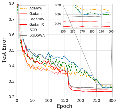
(a) VGG-16

(b) ResNeXt-29

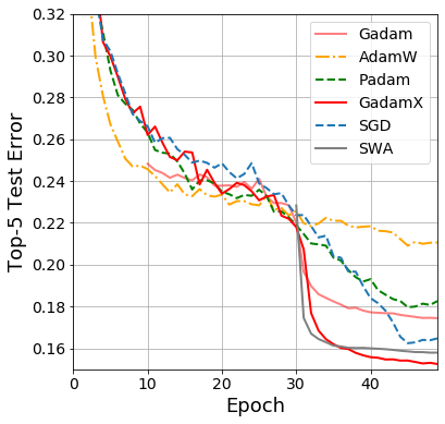
(c) WRN-28-10

Figure 5: (a-b) Top $1$ Test error on CIFAR-$100$, (c) Top-$5$ Test Error on ImageNet-$32$ and (d) IA test improvement over its base optimiser against number of parameters.

Table 3: ImageNet Results

Architecture	Optimiser	Top-1	Top-5
ResNet-50	SGD(step)	75.63	92.67
	SWA	76.32	93.15
	AdamW(lin)	74.04	91.57
	Ranger	75.64	92.53
	Gadam	76.79	93.21
	GadamX	77.31	93.47
ResNet-101	SGD (step)	77.37	93.78
	SWA	78.08	93.92
	AdamW(lin)	74.48	91.82
	Ranger	75.62	92.42
	Gadam	78.53	94.29
	GadamX	78.72	94.18

Table 4: CIFAR-$10$/$100$ Results

Architecture	Optimiser	C$10$ Test Acc	C$100$ Test Acc
VGG-16	SGD	94.14$\pm 0.37$	74.15$\pm 0.06$
	SWA	94.69$\pm 0.36$	74.57$\pm 0.27$
	Adam(W)	93.90 $\pm 0.11$	73.26$\pm 0.30$
	Padam(W)	94.13 $\pm 0.06$	74.56$\pm 0.19$
	Gadam	94.62$\pm 0.15$	75.73$\pm 0.29$
	GadamX	94.88$\pm 0.03$	76.85$\pm 0.08$
PRN-110	SGD	95.40$\pm 0.25$	77.22$\pm 0.05$
	SWA	95.55$\pm 0.12$	77.92$\pm 0.36$
	Adam(W)	94.69$\pm 0.14$	75.47$\pm 0.21$
	Padam(W)	95.28$\pm 0.13$	77.30 $\pm 0.11$
	Gadam	95.27$\pm 0.02$	77.37$\pm 0.09$
	GadamX	95.95$\pm 0.06$	77.90 $\pm 0.21$

7 ImageNet Experiments

We compare against step learning rate decay (factor of $10$ every $30$ epochs) and linear schedule for SGD and AdamW for $90$ epochs (He et al., 2016a), with respective initial learning rates $\alpha=0.1,0.001$ and weight decays $10^{-4},10^{-2}$ on ImageNet (Russakovsky et al., 2015). We combine LookAhead (Zhang et al., 2019b) with gradient centralisation (Yong et al., 2020) as a high performance adaptive baseline  Ranger (Wright, 2019), also using step decay. We search for the best performing initial learning rates for SGD, AdamW, SWA, GadamX and Ranger by factors of $3$ i.e $0.001,0.003$ in either direction (increase/decrease) until we find a local maximum in performance, otherwise leaving settings as in Section 6. We show the results in Table 4.

Experimenting with Partial Adaptivity for the Best Computer Vision Results:

Following Granziol et al. (2020a); Choi et al. (2019), we experiment with setting the numerical stability coefficient to $\delta=10^{-4}$ instead of $10^{-8}$ for GadamX and attempt an SGD like procedure for Gadam where we train with $\alpha=0.5,\delta=1,\gamma=10^{-4}$. Note that such a large numerical stability coefficient has a similar effect to reducing the effect of the preconditioning matrix as GadamX hence also allowing for a larger global learning rate. We find that whilst the generalisation benefit of using Gadam alone is significant (without decreasing partial adaptivity) it is not competitive with SGD on this dataset, wheras leaving the numerical stability coefficient unchanged for GadamX only results in a very minor decrease in performance. We detail both of these effects in experimental finding $3$.

Due to poor out of the box performance of SWA, we repeat the logarithmic grid search procedure on the IA learning rate for SWA. We report results in Table 4, where we see Gadam(X) strongly out-performing all baselines. We do not include the ResNet-$18$ as AdamW outperforms SGD with $69.92\%$ top-$1$ accuracy over $69.72\%$, hence not a useful test-case for analysing the adaptive generalisation gap, prevalent in deeper models. Gadam nonetheless improves on this attaining $70.11\%$. Whilst we find that step/linear scheduling is less effective for AdamW/SGD, attaining $73.68/75.52\%$ respectively on the ResNet-$50$. Since these are small difference we don’t consider scheduling to be a major factor in our outstanding results. We detail our major experimental findings from these experiments which could be of use to the community.

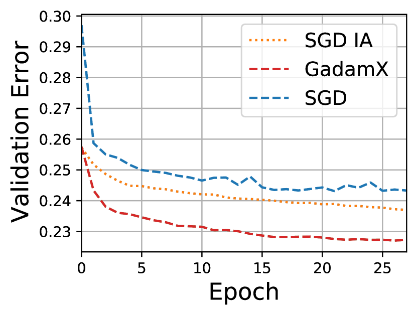
(a) ResNet-$50$

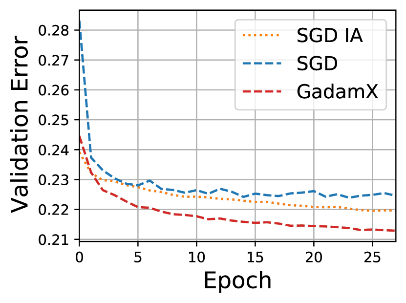
(b) ResNet-$101$

Figure 6: Final ImageNet epochs, showing the improvement of both SGD with Iterate Averaging (SGD IA) and our proposed GadamX optimiser over the SGD step-schedule in Top-$1$ validation error.

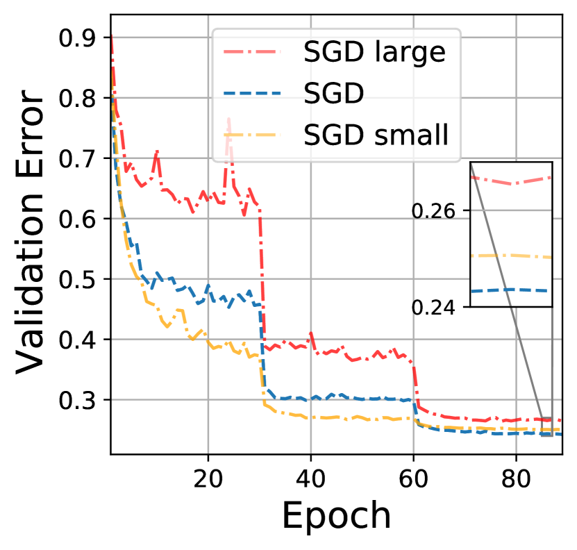
(a) SGD $\alpha=[0.03,0.1,0.3]$

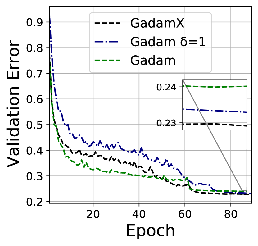
(b) Speed/Error Trade-off

Figure 7: (a) Unlike IA adaptive methods, SGD does not benefit from larger initial learning rates. (b) To attain the greatest generalisation with adaptive methods, the fast convergence is sacrificed. Gadam $\delta=1$, has a correspondingly large learning rate $0.5$

1. Adaptive IA makes use of huge initial learning rates:

unlike SGD and SWA, which have a strong performance degradation when large initial learning rates are used, shown in Fig 7(a), we find that large initial learning rates improve the generalisation performance of Gadam/GadamX, with the largest initial learning rates giving the best results.

2. Convergence speed comes at a cost:

Combining a large numerical stability coefficient and large learning rates allows Gadam to give significantly superior performance to SGD. However, the price paid is in convergence speed, shown in Fig 7(b). For these settings the convergence speed is often as slow or slower than GadamX. Using the same settings as in the small scale experiments (shown as Gadam in the graph) we achieve a top-$1$ accuracy of $75.52$ for ResNet-$50$. Whilst this significantly improves upon the base optimiser AdamW, these results are not as strong as those of SGD. Whilst increasing the base learning rate to $0.003$ increases the ResNet-$50$ Gadam generalisation performance to $76.53$, much of the convergence speed is already lost. We note that the effective weight decay is given by $(1-\alpha\gamma)$ so we expect higher regularisation from higher learning rates. We do not find that increasing the weight decay whilst keeping the same base learning rates produces as strong results in our experiments and hence this learning rate and weight decay interplay could form the basis for interesting future work.

3. Partially adaptive optimisation generalises best:

We find that for all experiments GadamX delivers the strongest performance. We do not find a strong dependence on the choice of the IA starting point (we try epoch $61,71,81$). We find that altering the numerical stability constant gives a small boost in Top-$1$ error, from $77.19$ to $77.31$ for the ResNet-$50$, but that results remain strong for the traditional setting.

Comparison to previous results:

We specifically report the final (as opposed to best) validation error for all our runs. We find the best SGD ResNet-$50$/$101$ results to be $75.75/77.62\%$, which are slightly worse/better than the official repository results. All of these results are still significantly lower than results achieved by Gadam/GadamX. We note that iterate averaged methods seem to continually decrease error in the final epochs of training, unlike SGD, which can sometimes overfit slightly in the final epochs of training.

8 Beyond Computer Vision: PTB LSTM

We run word-level language modelling using a 3-layer Long-short Term Memory (LSTM) model (Gers et al., 1999) on PTB dataset (Marcus et al., 1993) and the results are shown in Table 5 and Figure 8. Remarkably, Gadam achieves a test perplexity of 58.77 (58.61 if we tune $T_{\mathrm{avg}}$. See Table 6 in Section 10), better than the baseline NT-ASGD in Merity et al. (2017) that runs an additional 300 epochs on an identical network. Note that since, by default, the ASGD uses a constant learning rate, we do not schedule the learning rate except Padam which requires scheduling to converge. Also, for consistency, we use a manual trigger to start averaging at the 100th epoch for ASGD (which actually outperforms the NT-ASGD variant). We additionally conduct experiments with scheduling and NT-ASGD (appendix Section D) and Gadam still outperforms. It is worth mentioning that for state of the art results in language modelling Melis et al. (2017); Brown et al. (2020); Shoeybi et al. (2019), Adam is the typical optimiser of choice. Hence these results are both encouraging and significant for wider use in the community.

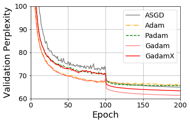
Figure 8: Validation perplexity of 3-layer LSTM on PTB word-level modelling

Data	Optimiser	Perplexity
		Validation	Test
PTB	ASGD	64.88$\pm 0.07$	61.98$\pm 0.19$
	Adam	65.96$\pm 0.08$	63.16$\pm 0.24$
	Gadam	61.35$\pm 0.05$	58.77$\pm 0.08$
	GadamX	63.49$\pm 0.19$	60.45$\pm 0.04$

Table 5: LSTM Penn Treebank Experimental results.

9 Effect of Frequency of Averaging

While we derive the theoretical bounds for both Polyak-style averaging on every iteration and strided averaging, in practice we use strided averaging to save on computation. We either average once per epoch similar to Izmailov et al. (2018), or select a rather arbitrary value such as averaging once per 100 iterations. The reason is both practical and theoretical: averaging much less leads to significant computational savings, and at the same time as we argued more independent iterates the benefit from averaging is better. In this case, averaging less causes the iterates to be further apart and more independent, and thus fewer number of iterates is required to achieve the similar level of performance if less independent iterates are used. We verify this both on the language and the vision experiments using the identical setup as the main text. With reference to Figure 9(a), not only is the final perplexity very insensitive to averaging frequency (note that the y-axis scale is very small), it is also interesting that averaging less actually leads to a slightly better validation perplexity compared to schemes that, say, average every iteration. We see a similar picture emerges in Figure 9(b), where the despite of following very close trajectories, averaging every iteration gives a slightly worse testing performance compared to once an epoch and is also significantly more expensive (with a NVIDIA GeForce RTX 2080 Ti GPU, each epoch of training takes around 10s if we average once per epoch but averaging every iteration takes around 20s).

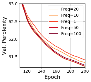
(a) LSTM on PTB

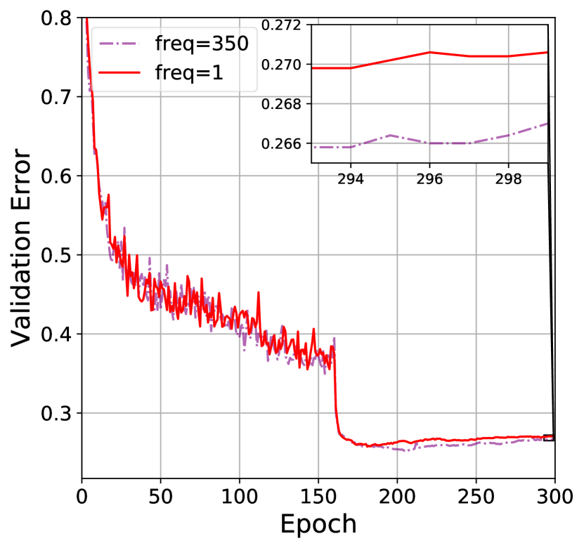
(b) VGG-16 on CIFAR-100

Figure 9: Effect of different averaging frequencies on validation perplexity of Gadam on representative (a) Language and (b) Image classification tasks. Freq=$n$ suggests averaging once per $n$ iterations. freq=350 in (b) is equivalently averaging once per epoch.

10 Effect of Average Starting Point and GadamAuto

In Gadam(X), we need to determine when to start averaging ($T_{\mathrm{avg}}$ in Algorithm 1), and here we investigate the sensitivity of Gadam(X) to this hyperparameter. We use a range of $T_{\mathrm{avg}}$ for a number of different tasks and architectures (Figure 10 and Table 6), including extreme choices such as $T_{\mathrm{avg}}=0$ (start averaging at the beginning). We observe that for any reasonable $T_{\mathrm{avg}}$, Gadam(X) always outperform their base optimisers with standard learning rate decay, and tuning $T_{\mathrm{avg}}$ yields even more improvements over the heuristics employed in the main text, even if selecting any sensible $T_{\mathrm{avg}}$ already can lead to a promising performance over standard learning rate decay.

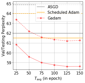
(a) LSTM. dashed/solid lines denote val/test perp.

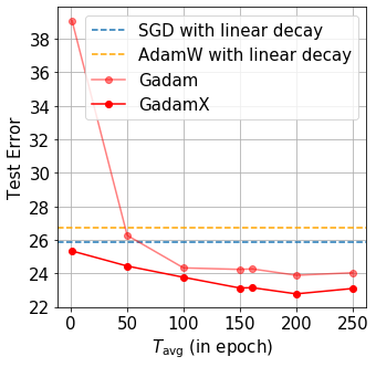
(b) VGG-16 on CIFAR-100

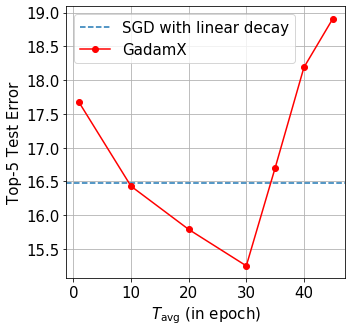
(c) WRN-28-10 on ImageNet 32$\times$32

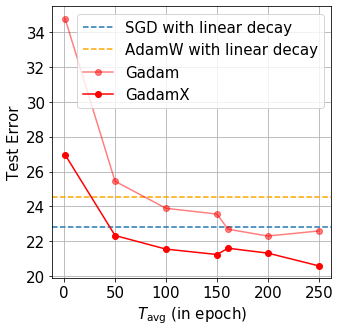
(d) PRN-110 on CIFAR-100

Figure 10: Effect of different $T_{\mathrm{avg}}$ on the performance of various tasks and architectures.

Table 6: Best results obtained from tuning $T_{\mathrm{avg}}$

Architecture	Optimiser	Test Acc./Perp.
CIFAR-100
VGG-16	Gadam	76.11
	GadamX	77.22
PRN-110	Gadam	77.41
	GadamX	79.41
ImageNet 32$\times$32
WRN-28-10	GadamX	84.75
PTB
LSTM	Gadam	58.61

Here we also conduct preliminary experiments on GadamAuto, a variant of Gadam that uses a constant learning rate schedule and automatically determines the starting point of averaging and training termination - this is possible given the insensitivity of the end-results towards $T_{\mathrm{avg}}$ as shown above, and is desirable as the optimiser both has fewer hyperparameters to tune and trains faster. We use VGG-16 network on CIFAR-100. For all experiments, we simply use a flat learning rate schedule. The results are shown in Table 7. We use a patience of 10 for both the determination of the averaging activation and early termination. We also include SWA experiments with SGD iterates.

Table 7: GadamAuto Test Performance at Termination.

Optimiser	Data-set	Test Accuracy
Gadam-Auto	CIFAR-100	75.39
SWA-Auto	CIFAR-100	73.93

It can be seen that, while automatic determination for averaging trigger and early termination work well for Gadam (GadamAuto posts a performance only marginally worse than the manually tuned Gadam), they lead to a rather significant deterioration in test in SWA (SWA-Auto performs worse than tuned SWA, and even worse than tuned SGD). This highlights the benefit of using adaptive optimiser as the base optimiser in IA, as the poor performance in SWA-Auto is likely attributed to the fact that SGD is much more hyperparameter-sensitive (to initial learning rate and learning rate schedule, for example. SWA-Auto uses a constant schedule, which is sub-optimal for SGD), and that validation performance often fluctuates more during training for SGD: SWA-Auto determines averaging point based on the number of epochs of validation accuracy stagnation. For a noisy training curve, averaging might be triggered too early; while this can be ameliorated by setting a higher patience, doing so will eventually defeat the purpose of using an automatic trigger. Both issues highlighted here are less serious in adaptive optimisation, which likely leads to the better performance of GadamAuto.

Nonetheless, the fact that scheduled Gadam still outperforms GadamAuto suggests that there is still ample room of improvement to develop a truly automatic optimiser that performs as strong as or even stronger than tuned ones. One desirable alternative we propose for the future work is the integration of Rectified Adam Liu et al. (2019), which is shown to be much more insensitive to choice of hyperparameter even compared to Adam.

11 Conclusion

We propose a Gaussian Process perturbation between the batch and true risk surfaces and derive the phenomenon of improved generalisation for large learning rates and larger weight decay when combined with iterate averaging observed in practice. We extend this formalism to include adaptive methods and show that we expect further improvement when using adaptive algorithms. Based on this theory we develop two adaptive algorithms, Gadam and GadamX, variants of Adam with iterate averaging. We extensively validate Gadam and GadamX on computer vision tasks and a natural language experiment, showing strong performance against baseline and state of the art. Another interesting consequence of our work is that in all our experiments the last iterate is the best. Unlike SGD, where the epoch of best test/validation error is typically not the last and techniques such as early stopping are often employed, we find consistent near-monotonic improvements in test/validation error using our algorithms. We also find from preliminary analysis that our algorithms require less hyper-parameter tuning than SGD and variants thereof. This may be of interest for practitioners that want to get good results fast, as opposed to state of the art slowly.

A Proofs

In this section we give any proofs that were omitted from the main text.

A.1 Proof of Theorem 5

The proof of Theorem 5 was given in the main text but depends on several intermediate results which we now state and prove.

Lemma 9

Take any ${\bm{x}}_{0},\ldots,{\bm{x}}_{n-1}\in\mathbb{R}^{P}$ let ${\bm{X}}\sim\mathcal{N}(0,\sigma^{2}I)$. Consider $P\rightarrow\infty$ with $P\gg\log{n}$ and let $\delta>0$ be $o(P^{\frac{1}{2}})$ (note that $\delta$ and $n$ need not diverge with $P$, but they can). Define

$$B_{i}=\{{\bm{x}}\in\mathbb{R}^{P}\mid||{\bm{x}}-{\bm{x}}_{i}||<\delta\},$$

then as $P\rightarrow\infty$

$$\mathbb{P}\left({\bm{X}}\in\bigcup_{i}B_{i}\right)\rightarrow 0$$ (50)

and moreover as $P,n\rightarrow\infty$

$$n\mathbb{P}\left({\bm{X}}\in\bigcup_{i}B_{i}\right)\rightarrow 0.$$ (51)

Proof  With the Euclidean volume measure, we have

$$Vol\left(\bigcup_{i}B_{i}\right)\leq nV_{P}\delta^{P}=V_{P}(\delta n^{1/P})^{P}$$

where $V_{P}$ is the volume of the unit sphere in $P$ dimensions. Therefore

$$\mathbb{P}\left({\bm{X}}\in\bigcup_{i}B_{i}\right) \leq\frac{1}{(2\pi\sigma^{2})^{\frac{P}{2}}}\frac{2\pi^{\frac{P}{2}}}{\Gamma(\frac{P}{2})}\int_{0}^{\delta n^{\frac{1}{P}}}dr~{}e^{-\frac{r^{2}}{2\sigma^{2}}}r^{P-1}$$

$$=\frac{2}{\Gamma(\frac{P}{2})}\int_{0}^{\frac{\delta n^{\frac{1}{P}}}{\sqrt{2}\sigma}}dr~{}e^{-r^{2}}r^{P-1}$$

$$=\frac{1}{\Gamma(\frac{P}{2})}\int_{0}^{\frac{\delta n^{\frac{2}{P}}}{2\sigma^{2}}}dr~{}e^{-r}r^{\frac{P}{2}-1}$$

$$=\frac{1}{\Gamma(\frac{P}{2})}\gamma\left(\frac{P}{2};\frac{n^{\frac{2}{P}}\delta^{2}}{2\sigma^{2}}\right)$$ (52)

where $\gamma$ is the lower incomplete gamma function. Since $P\gg\log{n}$ and $\delta=o(P^{\frac{1}{2}})$, it follows that

$$\frac{n^{\frac{2}{P}}\delta^{2}}{2\sigma^{2}}=o(P)$$

and so Lemma 10 can be applied to yield the result, recalling that $n\ll e^{P}$.  

Lemma 10

Define the function

$$r(a;x)=\frac{\gamma(a;x)}{\Gamma(a)},$$ (53)

where $\gamma$ is the lower incomplete gamma function. Assume that $a\ll x$, where $x$ may or may not diverge with $a$, then as $a\rightarrow\infty$, $r(a;x)\rightarrow 0$, and more precisely

$$r(a;x)\sim\frac{1}{\sqrtsign{2\pi}}\exp\left(-x+a\log{x}-a-a\log{a}-\frac{1}{2}\log{a}\right).$$ (54)

Proof  We have $\gamma(a;x)=a^{-1}x^{a}\,_{1}F_{1}(a;1+a;-x)$, where $\,{}_{1}F_{1}$ is the confluent hypergeometric function of the first kind (Andrews et al., 1999). Then

$$r(a;x) =\frac{a^{-1}x^{a}\,_{1}F_{1}(a;1+a;-x)}{\Gamma(a)}=\frac{a^{-1}x^{a}\Gamma(a+1)}{\Gamma(a)^{2}}\int_{0}^{1}e^{xt}t^{a-1}dt$$ (55)

where we have used a result of Abramowitz et al. (1988). The integral in (55) can be evaluated asymptotically in the limit $x\rightarrow\infty$ with $x\ll a$. Writing the integrand as $e^{xt+(a-1)\log{t}}$ it is plainly seen to have no saddle points in $[0,1]$ given the condition $x\ll a$. The leading order term therefore originates at the right edge $t=1$. A simple application of Laplace’s method leads to

$$r(a;x) \sim\frac{a^{-1}x^{a}\Gamma(a+1)e^{-x}}{\Gamma(a)^{2}(a-1-x)}$$

$$\sim\frac{x^{a}e^{-x}}{a\Gamma(a)}$$

$$\sim\frac{x^{a}e^{-x}}{a\sqrtsign{2\pi a^{-1}}(ae^{-1})^{a}}$$

$$=\frac{1}{\sqrtsign{2\pi}}\exp\left(-x+a\log{x}-a-a\log{a}-\frac{1}{2}\log{a}\right)$$

where the penultimate line makes uses of Stirling’s approximation (Andrews et al., 1999). Since $a\gg x$,

$$-x+a\log{x}-a-a\log{a}-\frac{1}{2}\log{a}\sim-a\log{a}\rightarrow-\infty$$

which completes the proof.  

The following two lemmas were stated in the main text. Their proofs, which we now give, depend on the preceding lemmas.

Proof of Lemma 3  Let us use the definitions of $B_{i}$ from Lemma 9 (with ${\bm{X}}_{i}$ replacing ${\bm{x}}_{i}$ and ${\bm{X}}$ in the obvious way). Since $A_{i}(\delta)\subset A_{i-1}(\delta)$, the chain rule of probability gives

$$\mathbb{P}(A_{n}(\delta)) =\mathbb{P}\left(\bigcap_{i\leq n}A_{i}(\delta)\right)=\mathbb{P}(A_{1}(\delta))\prod_{i=1}^{n-1}\mathbb{P}(A_{i}\mid A_{i-1})$$

but

$$\mathbb{P}(A_{i}(\delta)\mid A_{i-1}(\delta))=1-\mathbb{P}\left({\bm{X}}_{i}\in\bigcup_{j<i}B_{j}\right)$$

and so (51) gives the result.  

Proof of Lemma 4  Each of the ${\bm{\epsilon}}_{i}$ is Gaussian distributed with covariance matrix $\mathrm{Cov}({\bm{\epsilon}}_{i})$ given by Equation $6$ and the covariance between different gradients $\mathrm{Cov}({\bm{\epsilon}}_{i},{\bm{\epsilon}}_{j})$ is similarly given by Equation $6$. By standard multivariate Gaussian properties

$$\mathrm{Cov}(\bar{{\bm{\epsilon}}}) =\sum_{i=1}^{n}a_{i}^{2}~{}\mathrm{Cov}({\bm{\epsilon}}_{i})+\sum_{i\neq j}a_{i}a_{j}\mathrm{Cov}({\bm{\epsilon}}_{i},{\bm{\epsilon}}_{j}),$$ (56)

then taking the trace

$$\operatorname{Tr}~{}\mathrm{Cov}(\bar{{\bm{\epsilon}}}) =\sum_{i=1}^{n}a_{i}^{2}\operatorname{Tr}(\mathrm{Cov}({\bm{\epsilon}}_{i}))+2\sum_{1\leq i<j\leq n}a_{i}a_{j}\operatorname{Tr}(\mathrm{Cov}({\bm{\epsilon}}_{i},{\bm{\epsilon}}_{j})).$$ (57)

Using the covariance structure from (18) in the main text gives

$$\operatorname{Tr}~{}\mathrm{Cov}(\bar{{\bm{\epsilon}}})=k^{\prime}(0)\sum_{i=1}^{n}a_{i}^{2}\operatorname{Tr}{I}+2\sum_{1\leq i<j\leq n}a_{i}a_{j}\Bigg{[} k^{\prime}(-\frac{d_{ij}^{2}}{2})\operatorname{Tr}{I}$$

$$+k^{\prime\prime}(-\frac{d_{ij}^{2}}{2})\operatorname{Tr}({\bm{w}}_{i}-{\bm{w}}_{j})({\bm{w}}_{j}-{\bm{w}}_{i})^{T}\Bigg{]}$$ (58)

from which the result follows.  

A.2 Proofs of Theorem 7 and Corollary 6

Both of the proofs given here are quite similar to the proof of Theorem 5 in the main text and so we here present only the differences.

Proof of Theorem 7  The proof is much the same as that of Theorem 5, except a slightly modified version of Lemma 4 is required. The expression analogous to the result in that lemma is different in the following two ways:

1. All terms are divided by positive powers of $\|{\bm{w}}\|_{2}$.

2. There are extra terms arising from derivatives applied to $||{\bm{w}}||_{2}^{-1}$, which give rise to factors of the form ${\bm{w}}_{i}^{T}({\bm{w}}_{j}-{\bm{w}}_{j})$.

Extending the proof of Theorem 5 to this case requires the following two observations. Firstly, terms of the form ${\bm{w}}_{i}^{T}({\bm{w}}_{j}-{\bm{w}}_{j})$ can be easily bounded as $|{\bm{w}}_{i}^{T}({\bm{w}}_{j}-{\bm{w}}_{j})|\leq||{\bm{w}}||_{2}d_{ij}$. Secondly the terms of the form $||{\bm{w}}||_{2}^{-r}$ for $r\geq 1$ will cause no problems so long as they can be uniformly bounded away from $0$ as $P,n\rightarrow\infty$. This can be established with high probability as a trivial extension of Lemma 3 by introducing an extra point ${\bm{X}}_{0}$, say, at the origin.  

Proof of Corollary 6  The proof is just as in Theorem $2$ (or Theorems $3$ or $4$), differing only in the values of the $\bar{a}_{i}$. Indeed, a little thought reveals that the generalisation of $\bar{a}_{i}$ to the case $\kappa>1$ is

$$\bar{a}_{i}=\frac{\alpha\kappa}{n}(1-\alpha\lambda)^{\kappa\left(1+\lfloor\frac{i}{\kappa}\rfloor\right)-1-i}\frac{1-(1-\alpha\lambda)^{\kappa\left(\lfloor\frac{n}{\kappa}\rfloor-\lfloor\frac{i}{\kappa}\rfloor\right)}}{1-(1-\alpha\lambda)^{\kappa}}.$$ (59)

Note that $\kappa\left\lfloor\frac{i}{\kappa}\right\rfloor-i$ is just the (negative) remainder after division of $i$ by $\kappa$. Then for large $n$

$$\sum_{i}\bar{a}_{i}^{2} \sim\frac{\alpha^{2}\kappa^{2}}{n^{2}}\frac{(1-\alpha\lambda)^{2(\kappa-1)}}{\left(1-(1-\alpha\lambda)^{\kappa}\right)^{2}}\left\lfloor\frac{n}{\kappa}\right\rfloor\sum_{i=0}^{\kappa-1}(1-\alpha\lambda)^{-2i}$$

$$\leq\frac{\alpha^{2}\kappa}{n}\frac{(1-\alpha\lambda)^{2(\kappa-1)}}{\left(1-(1-\alpha\lambda)^{\kappa}\right)^{2}}\sum_{i=0}^{\kappa-1}(1-\alpha\lambda)^{-2i}$$

$$=\frac{\alpha^{2}\kappa}{n}\frac{(1-\alpha\lambda)^{2(\kappa-1)}}{\left(1-(1-\alpha\lambda)^{\kappa}\right)^{2}}\frac{1-(1-\alpha\lambda)^{-2\kappa}}{1-(1-\alpha\lambda)^{-2}}$$

$$=\frac{\alpha^{2}\kappa}{n}\frac{1}{\left(1-(1-\alpha\lambda)^{\kappa}\right)^{2}}\frac{1-(1-\alpha\lambda)^{2\kappa}}{1-(1-\alpha\lambda)^{2}}.$$

and similarly

$$\sum_{i<j}\bar{a}_{i}\bar{a}_{j} \sim\frac{\alpha^{2}\kappa^{2}}{n^{2}}\frac{(1-\alpha\lambda)^{2(\kappa-1)}}{(1-(1-\alpha\lambda)^{\kappa})^{2}}\sum_{i<j}(1-\alpha\lambda)^{\kappa\lfloor i/\kappa\rfloor-i+\kappa\lfloor j/\kappa\rfloor-j}$$ (60)

$$\sim\frac{\alpha^{2}\kappa^{2}}{n^{2}}\frac{(1-\alpha\lambda)^{2(\kappa-1)}}{(1-(1-\alpha\lambda)^{\kappa})^{2}}\sum_{j}(1-\alpha\lambda)^{\kappa\lfloor j/\kappa\rfloor-j}\left\lfloor\frac{j}{\kappa}\right\rfloor\frac{1-(1-\alpha\lambda)^{-\kappa}}{1-(1-\alpha\lambda)^{-1}}$$ (61)

$$\sim\frac{\alpha^{2}\kappa^{2}}{n^{2}}\frac{(1-\alpha\lambda)^{2(\kappa-1)}}{(1-(1-\alpha\lambda)^{\kappa})^{2}}\left(\frac{1-(1-\alpha\lambda)^{-\kappa}}{1-(1-\alpha\lambda)^{-1}}\right)^{2}\sum_{j=0}^{\lfloor n/\kappa\rfloor}j$$ (62)

$$\sim\frac{\alpha^{2}}{2}\frac{(1-\alpha\lambda)^{2(\kappa-1)}}{(1-(1-\alpha\lambda)^{\kappa})^{2}}\left(\frac{1-(1-\alpha\lambda)^{-\kappa}}{1-(1-\alpha\lambda)^{-1}}\right)^{2}$$ (63)

$$=\frac{\alpha^{2}}{2}\frac{(1-\alpha\lambda)^{-2}}{(1-(1-\alpha\lambda)^{-1})^{2}}.$$ (64)

 

B Gadam and Lookahead

As discussed, most related works improve generalisation of adaptive methods by combining them with SGD in some form. As an example representing the recent works claiming promising performances, Chen and Gu (2018) introduce an additional hyperparameter $p$, to control the extent of adaptivity: for $p=\{\frac{1}{2},0\}$, we have fully adaptive Adam(W) or pure first-order SGD respectively and usually a $p$ falling between the extremes is taken. In addition to empirical comparisons, since our approach is orthogonal to these approaches, as an singular example, we propose GadamX that combines Gadam with Padam, where for simplicity we follow Chen and Gu (2018) to fix $p=\frac{1}{8}$ for the current work. We note that $p<1$ is regularly considered a heuristic to be used for an inaccurate curvature matrix Martens (2014), although the specific choice of $p=1/2$ has a principled derivation in terms of a regret bound Duchi et al. (2011). Previous works also use EMA in weight space to achieve optimisation and/or generalisation improvements: Izmailov et al. (2018) entertain EMA in SWA, although they conclude simple averaging is more competitive. Recently, Zhang et al. (2019b) proposes Lookahead (LH), a plug-in optimiser that uses EMA on the slow weights to improve convergence and generalisation. Nonetheless, having argued the dominance of noise in the high-dimensional deep learning regime, we argue that simple averaging is more theoretically desirable for generalisation. Following the identical analysis to the noisy quadratic with i.i.d noise, we consider the $1D$ case without loss of generality and denote $\rho\in[0,1]$ as the coefficient of decay, asymptotically the EMA point ${\bm{w}}_{\mathrm{ema}}$ is governed by:

$$\mathcal{N}\bigg{(}\frac{(1-\rho)w_{0}(1-\alpha\lambda)^{n+1}[1-(\frac{\rho}{1-\alpha\lambda})^{n-1}]}{1-\alpha\lambda-\rho},\frac{1-\rho}{1+\rho}\frac{\alpha\sigma^{2}\kappa}{\lambda}\bigg{)}$$ (65)

Where $\kappa=(1-(1-\alpha\lambda)^{n-2})$). An alternative analysis of EMA arriving at similar result was done in Zhang et al. (2019a), but their emphasis of comparison is between the EMA and iterates instead of EMA and the IA point in our case. From (65), while the convergence in mean is less strongly affected, the noise is reduced by a factor of $\frac{1-\rho}{1+\rho}$. So whilst we reduce the noise possibly by a very large factor, it does not vanish asymptotically. Hence viewing EMA or IA as noise reduction schemes, we consider IA to be far more aggressive. Secondly, EMA implicitly assumes that more recent iterates are better, or otherwise more important, than the previous iterates. While justified initially (partially explaining LH’s efficacy in accelerating optimisation), it is less so in the late stage of training. We nonetheless believe LH could be of great value. Like our proposed methods, LH features weight-space average to achieve optimisation and generalisation benefits, however LH maintains different update rules for the fast and slow weights, and uses exponentially moving average to update the parameters. In this section, we both comment on the key theoretical differences between Gadam and Lookahead and make some preliminary practical comparisons. We also offer an attempt to bring together the optimisation benefit of Lookahead and the generalisation benefit of Gadam, with promising preliminary results.

B.1 Major Differences between Gadam and Lookahead

Averaging Method

Lookahead opts for a more complicated averaging scheme: they determine the ‘fast’- and ‘slow’- varying weights during optimisation, and maintains an EMA to average the weight. On the other hand, Gadam uses a more straightforward simple average. As we discussed in the main text, EMA is more theoretically justified during the initial rather than later stage of training. This can also be argued from a Bayesian viewpoint following Maddox et al. (2019), who argued that iterates are simply the draws from the posterior predictive distribution of the neural network, where as averaging leads to a rough estimation of its posterior mean. It is apparent that if the draws from this distribution are equally good (which is likely to be the case if we start averaging only if validation metrics stop improving), assigning the iterates with an exponential weight just based on when they are drawn constitutes a rather arbitrary prior in Bayesian sense.

Averaging Frequency

Lookahead averages every iteration whereas in Gadam, while possible to do so as well, by default averages much less frequently. We detail our rationale for this in Section 9.

Starting Point of Averaging

While Lookahead starts averaging at the beginning of the training, Gadam starts averaging either from a pre-set starting point or an automatic trigger (for GadamAuto). While authors of Lookahead Zhang et al. (2019b) argue that starting averaging eliminates the hyperparameter on when to start averaging, it is worth noting that Lookahead also introduces two additional hyperparameters $\alpha$ and $k$, which are non-trivially determined from grid search (although the authors argue that the final result is not very sensitive to them).

We believe the difference here is caused by the different design philosophies of Gadam and Lookahead: by using EMA and starting averaging from the beginning, Lookahead benefits from faster convergence and some generalisation improvement whereas in Gadam, since the averages of iterates are not used during training to promote independece between iterates, Gadam does not additionally accelerate optimisation but, by our theory, should generalise better. As we will see in the next section, this theoretical insight is validated by the experiments and leads to combinable benefits.

Empirical Comparison

We make some empirical evaluations on CIFAR-100 data-set with different network architectures, and we use different base optimiser for Lookahead. For all experiments, we use the author-recommended default values of $k=5$ (number of lookahead steps) and $\alpha=0.5$. We focus on the combination of Lookahead and adaptive optimisers, as this is the key focus of this paper, although we do include results with Lookahead with SGD as the base optimiser.

We first test AdamW and SGD with and without Lookahead and the results are in Figure 11. Whilst SGD + LH outperforms SGD in final test accuracy by a rather significant margin in both architectures, Lookahead does not always lead to better final test accuracy in AdamW (although it does improve the convergence speed and reduce fluctuations in test error during training, which is unsurprising as EMA shares similar characteristics with IA in reducing sensitivity to gradient noise). On the other hand, it is clear that Gadam delivers both more significant and more consistent improvements over AdamW, both here and in the rest of the paper.

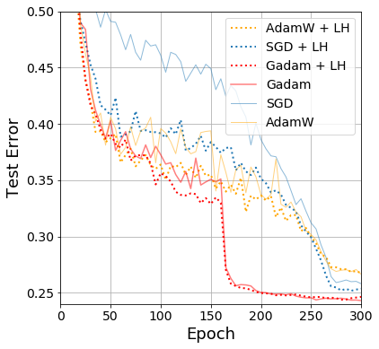
(a) VGG-16

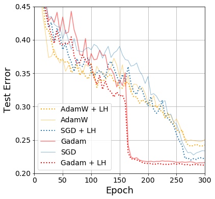
(b) PRN-110

Figure 11: Test accuracy of Lookahead in CIFAR-100 against number of epochs.

Nonetheless, we believe that Lookahead, being an easy-to-use plug-in optimiser that clearly improves convergence speed, offers significant combinable potential with Gadam, which focuses on generalisation. Indeed, by using Lookahead before the 161st epoch where we start IA, and switching to IA after the starting point, we successfully combine Gadam and LH into a new optimiser which we term Gadam + LH. With reference to Figure 11, in VGG-16, Gadam + LH both converges at the fastest speed in all the optimisers tested and achieves a final test accuracy only marginally worse than Gadam (but still stronger than all others). On the other hand, in PRN-110, perhaps due to the specific architecture choice, the initial difference in convergence speed of all optimisers is minimal, but Gadam + LH clearly performs very promisingly in the end: it is not only stronger than our result without Lookahead in Figure 11(b), but also, by visual inspection, significantly stronger than the SGD + LH results on the same data-set and using the same architecture reported in the original Lookahead paper Zhang et al. (2019b).

Due to the fact that Lookahead is a very recent creation and our constraint on computational resources, we have not been able to fully test Gadam + LH on a wider range of problems. Nonetheless, we believe that the results obtained here are encouraging, and should merit more in-depth investigations in the future works.

C Experiment Setup

Unless otherwise stated, all experiments are run with PyTorch 1.1 on Python 3.7 Anaconda environment with GPU acceleration. We use one of the three possible GPUs for our experiment: NVIDIA GeForce GTX 1080 Ti, GeForce RTX 2080 Ti or Tesla V100. We always use a single GPU for any single run of experiment.

C.1 Validating Experiments

VGG-16 on CIFAR-100

In this expository experiment, we use the original VGG-16 without batch normalisation (batch normalisation has non-trivial impact on conventional measures of sharpness and flatness. See Li et al. (2018)). We conduct all experiments with initial learning rate $0.05$. For fair comparison to previous literature, we use the linear decay schedules advocated in Izmailov et al. (2018), for both SGD and IA. For IA we run the set of terminal learning rates during averaging $\{0.03,0.01,0.003\}$, whereas for SGD we decay it linearly to $0.0005$

Table 8: Baseline Results from Previous Works

Network	Optimiser	Accuracy/Perplexity	Reference
CIFAR-100
VGG-16	SGD	73.80	Huang and Wang (2018)
VGG-16	FGE	74.26	Izmailov et al. (2018)
PRN-164	SGD	75.67	He et al. (2016b)
PRN-110	SGD	76.35	online repository**
ResNet-164	FGE	79.84	Izmailov et al. (2018)
ResNeXt-29	SGD	82.20	Xie et al. (2017)
ResNeXt-29	SGD	81.47	Bansal et al. (2018)
CIFAR-10
VGG-19	SGD	93.34	online repository**
VGG-16	SGD	93.90	Huang and Wang (2018)
PRN-110	SGD	93.63	He et al. (2016b)
PRN-110	SGD	95.06	online repository**
ImageNet 32$\times$32
WRN-28-10	SGD	59.04/81.13*	Chrabaszcz et al. (2017)
Modified WRN	SGD	60.04/82.11*	McDonnell (2018)
PTB
LSTM 3-layer	NT-ASGD	61.2/58.8***	Merity et al. (2017)
Notes:
* Top-1/Top-5 Accuracy
** Link: https://github.com/bearpaw/pytorch-classification
*** Validation/Test Perplexity

C.2 Language Modelling Experiments

In language modelling experiments, we use the codebase provided by https://github.com/salesforce/awd-lstm-lm. For ASGD, we use the hyperparameters recommended by Merity et al. (2017) and set the initial learning rate to be 30. Note that in language experiments, consistent with other findings decoupled weight decay seems to be not as effective $L_{2}$, possibly due to LSTM could be more well-regularised already, and that batch normalisation, which we argue to be central to the efficacy of decoupled weight decay, is not used in LSTM. Thus, for this set of experiments we simply use Adam and Padam as the iterates for Gadam and GadamX. For Adam/Gadam, we tune the learning rate by searching initial learning rate in the range of $\{0.0003,0.001,0.003,0.01\}$ and for Padam and GadamX, we set the initial learning rate to be $1$ and partially adaptive parameter $p=0.2$, as recommended by the authors Chen and Gu (2018). We further set the weight decay to be their recommended value of $1.2\times 10^{-6}$. For the learning rate schedule, we again follow Merity et al. (2017) for a piece-wise constant schedule, and decay the learning rate by a factor of $10$ at the $\{100,150\}$-th epochs for all experiments without using iterate averaging. For experiments with iterate averaging, instead of decaying the learning rate by half before averaging starts, we keep the learning rate constant throughout to make our experiment comparable with the ASGD schedule. We run all experiments for $200$ (instead of $500$ in Merity et al. (2017)) epochs.

Learning Rate Schedule

As discussed in the main text, the experiments shown in Table 10 and Figure 8 are run with constant schedules (except for Padam). Padam runs with a step decay of factor of 10 at $\{100,150\}$-th epochs. However, often even the adaptive methods such as Adam are scheduled with learning rate decay for enhanced performance. Therefore, we also conduct additional scheduled experiments with Adam, where we follow the same schedule of Padam. The results are shown in appendix Section D.2.

C.3 Experiment Baselines

To validate the results we obtain and to make sure that any baseline algorithms we use are properly and fairly tuned, we also survey the previous literature for baseline results where the authors use same (or similar) network architectures on the same image classification/language tasks, and the comparison of our results against theirs is presented in Table 8. It is clear that for most of the settings, our baseline results achieve similar or better performance compared to the previous work for comparable methods; this validates the rigour of our tuning process.

D Additional Experimental Results

D.1 Testing Performance of CIFAR-10

We report the testing performance of VGG-16 and PRN-110 on CIFAR-10 in Figure 12 and Table 9. Perhaps due to the fact that CIFAR-10 poses a simpler problem compared to CIFAR-100 and ImageNet in the main text, the convergence speeds of the optimisers differ rather minimally. Nonetheless, we find that GadamX still outperforms all other optimisers by a non-trivial margin in terms of final test accuracy.

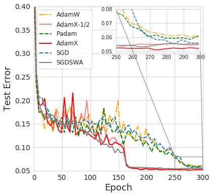
(a) VGG-16

(b) PRN-110

Figure 12: Test Error on CIFAR-10

Table 9: Top-1 Test Accuracy on CIFAR-10 Data-set

Architecture	optimiser	Test Accuracy
VGG-16	SGD	94.14$\pm 0.37$
	SWA	94.69$\pm 0.36$
	Adam(W)	93.90 $\pm 0.11$
	Padam(W)	94.13 $\pm 0.06$
	Gadam	94.62$\pm 0.15$
	GadamX	94.88$\pm 0.03$
PRN-110	SGD	95.40$\pm 0.25$
	SWA	95.55$\pm 0.12$
	Adam(W)	94.69$\pm 0.14$
	Padam(W)	95.28$\pm 0.13$
	Gadam	95.27$\pm 0.02$
	GadamX	95.95$\pm 0.06$

D.2 Word Level Language Modelling with Learning Rate Schedules and Non-monotonic Trigger

Word-level Language Modelling on PTB

Table 10: Validation and Test Perplexity on Word-level Language Modelling.

Data-set	optimiser	Perplexity
		Validation	Test
PTB	ASGD	64.88$\pm 0.07$	61.98$\pm 0.19$
	Adam	65.96$\pm 0.08$	63.16$\pm 0.24$
	Padam	65.69$\pm 0.07$	62.15$\pm 0.12$
	Gadam	61.35$\pm 0.05$	58.77$\pm 0.08$
	GadamX	63.49$\pm 0.19$	60.45$\pm 0.04$

Here we include additional results on word-level language modelling using scheduled Adam and NT-ASGD, where the point to start averaging is learned non-monotonically and automatically. Where scheduling further improves the Adam performance marginally, the automatically triggered ASGD actually does not perform as well as the manually triggered ASGD that starts averaging from 100th epoch onwards, as we discussed in the main text - this could be because that ASGD converges rather slowly, the 200-epoch budget is not sufficient, or the patience (we use patience = 10) requires further tuning. Otherwise, our proposed Gadam and GadamX without IA schedules still outperform the variants tested here without careful learning rate scheduling. The results are summarised in Figure 13 and Table 11.

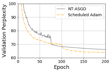
Figure 13: Validation Perplexity of NT-ASGD and Scheduled Adam on 3-layer LSTM PTB Word-level Modelling.

Table 11: Validation and Test Perplexity on Word-level Language Modelling. The Gadam(X) results are lifted from Table 10.

Data-set	optimiser	Perplexity
		Validation	Test
PTB	NT-ASGD	66.01	64.73
	Scheduled Adam	63.99	61.51
	Gadam (Ours)	61.35	58.77
	GadamX (Ours)	63.49	60.45

D.3 Relation between Improvement from Averaging and Number of Parameters in Previous Work

In this section we demonstrate that our claim that there should be a dependence on number of parameters $P$ on the margin of improvement from averaging is also present in previous works that use IA or a related ensemble method. Here we use the results from Table 1 of Izmailov et al. (2018). Since the different network architectures are trained with different budget of epochs which make the direct comparison of SWA results difficult, we instead consider their FGE (Garipov et al., 2018) results which the author argue to have the similar properties to and that is actually approximated by SWA. We plot their result along with us in Figure 14. While we do not obtain a perfect linear relationship possibly due to a wide range of possible interfering factors such as difference in architecture, use of batch normalisation, choice of optimiser and hyperparameter tuning, again we nevertheless observe that there exists a roughly positive relationship between $P$ and the margin of test improvement.

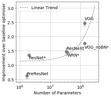
Figure 14: Number of parameters $P$ against improvement margin for both results obtained by us and in Izmailov et al. (2018) (annotated with asterisks) on CIFAR-100

D.4 Linear vs Step Scheduling

In this work, for the baseline methods in image classification tasks we use linear instead of the more conventionally employed step scheduling because we find linear scheduling to generally perform better in the experiments we conduct. In this section, we detail the results of these experiments, and in this section, ‘linear’ refers to the schedule introduced in appendix Section LABEL:sec:imagedetails and ‘step’ refers to the schedule that reduces the learning rate by a factor of 10 in $\{150,250\}$ epochs for 300-epoch experiments (CIFAR datasets), or in $\{25,40\}$ epochs for 50-epoch experiments (ImageNet dataset). The results are shown in Table 12.

Table 12: Testing performance of linear and step learning rate schedules on baseline methods.

Architecture	Optimiser	Step	Linear
CIFAR-100
VGG-16	SGD	73.28	74.15
	AdamW	73.20	73.26
	Padam	74.46	74.56
PRN-110	SGD	77.23	77.22
	AdamW	75.27	75.47
	Padam	73.95	77.30

E Importance of Iterate Averaging for Convergence

We argue that despite of the universal practical use of the final iterate of optimisation, it is heuristically motivated and in most proofs of convergence, some form of iterative averaging is required and used implicitly to derive the theoretical bounds. For $\beta$-Lipschitz, convex empirical risks, denoted the (overall) loss $L$. The difference between the $t+1$’th iterate and the optimal solution $L_{{\bm{w}}}^{*}$ can be bounded. The sum of differences along the trajectory (known as the regret) telescopes, hence resulting in a convergence rate for the average regret which is an upper bound for the loss of the average point Nesterov (2013); Duchi (2018):

$$\delta L=L_{{\bm{w}}_{t+1}}-L_{{\bm{w}}^{*}}\leq\nabla L_{{\bm{w}}_{t}}({\bm{w}}_{t+1}-{\bm{w}}^{*})+\frac{\beta}{2}||{\bm{w}}_{t+1}-{\bm{w}}_{t}||^{2}$$ (66)

$$\mathbb{E}(\delta L)\leq\hat{\nabla}L_{{\bm{w}}_{t}}({\bm{w}}_{t}-{\bm{w}}^{*})-(\alpha-\frac{\beta\alpha^{2}}{2})||\hat{\nabla}L_{{\bm{w}}_{t}}||^{2}+\alpha\sigma^{2}_{t}$$

where $\hat{\nabla}L_{{\bm{w}}_{t}}$ is the noisy gradient at ${\bm{w}}_{t}$ and $\sigma^{2}_{t}$ is its variance: $\text{Var}(\hat{\nabla}L_{{\bm{w}}_{t}})$. Noting that ${\bm{w}}_{t+1}={\bm{w}}_{t}-\alpha\hat{\nabla}L_{{\bm{w}}_{t}}$:

$$\frac{R}{T} =\mathbb{E}\Big{[}\frac{1}{T}\sum_{t=1}^{T-1}L_{{\bm{w}}_{t+1}}-L_{{\bm{w}}^{*}}\Big{]}$$ (67)

Using Jensen’s inequality, we have:

$$\frac{R}{T} \leq\frac{1}{T}\sum_{t=0}^{T-1}\frac{||{\bm{w}}_{t}-{\bm{w}}^{*}||^{2}-||{\bm{w}}_{t+1}-{\bm{w}}^{*}||^{2}}{2\alpha}+\alpha\sigma^{2}_{t}$$ (68)

$$\mathbb{E}[L_{\frac{1}{T}\sum_{t=1}^{T-1}{\bm{w}}_{t+1}}-L_{{\bm{w}}^{*}}]\leq\frac{R}{T}\leq\frac{||{\bm{w}}_{0}-{\bm{w}}^{*}||^{2}}{2\alpha T}+\alpha\sigma^{2}_{m}$$

where $\sigma^{2}_{m}=\operatorname*{arg\,max}_{{\bm{w}}_{t}}\mathbb{E}||\hat{\nabla}L_{{\bm{w}}_{t}}-\nabla L_{{\bm{w}}_{t}}||^{2}$, and $R$ is the regret. Setting $\alpha=(\beta+\sigma\frac{\sqrt{T}}{D})^{-1}$ in equation 67 gives us the optimal convergence rate. Similar convergence results can be given for a decreasing step size $\alpha_{t}\propto t^{-1/2}\alpha_{0}$. For adaptive optimisers, the noisy gradient is preconditioned by some non-identity matrix $\bar{\bm{B}}^{-1}$:

$${\bm{w}}_{k+1}\leftarrow{\bm{w}}_{k}-\alpha\bar{\bm{B}}^{-1}\nabla L_{k}({\bm{w}})$$ (69)

Methods of proof Reddi et al. (2019); Tran et al. (2019) rely on bounding the regret $\mathcal{O}(\sqrt{T})$ and showing that the average regret $\frac{R}{T}\rightarrow 0$ and Equation 67 explicitly demonstrates that the average regret is an upper bound on the expected loss for the average point in the trajectory. Hence existing convergence results in the literature prove convergence for the iterate average, but not the final iterate.

E.0.1 Optimal Learning Rates

Setting $\alpha=(\beta+\sigma\frac{\sqrt{T}}{D})^{-1}$ gives us the optimal convergence rate of $\frac{\beta R^{2}}{T}+\frac{\sigma D}{\sqrt{T}}$. Similar convergence results can be given for a decreasing step size $\alpha_{t}\propto t^{-1/2}\alpha_{0}$ Duchi (2018) when the number of iterations $T$ is not known in advance. Given the use of both iterate averaging and learning rate schedule in the proofs, it is difficult to understand the relative importance of the two and how this compares with the typical heuristic of using the final point.

E.1 Relevance of Local Geometry Arguments

One argument as to why IA improves generalisation Izmailov et al. (2018) is about the local geometry of the solution found: Izmailov et al. (2018) discuss the better generalisation of SWA to the “flatter” minimum it finds. The same argument is used to explain the apparent worse generalisation of adaptive method: Wu et al. (2018) showed empirically that adaptive methods are not drawn to flat minima unlike SGD. From both Bayesian and minimum description length arguments Hochreiter and Schmidhuber (1997), flatter minima generalise better, as they capture more probability mass. He et al. (2019) formalise the intuition under the assumption of a shift between the training and testing loss surface and investigate the presence of “flat valleys” in loss landscape. They argue that averaging leads to a biased solution to the “flatter” valley, which has worse training but better generalisation performance due to the shift. This suggests IA has an inherent regularising effect, which contrasts with our previous claim that IA should improve both.

However, one issue in the aforementioned analysis, is that they train their SGD baseline and averaged schemes on different learning rate schedules. While this is practically justified, and even desirable, exactly because IA performs better with high learning rate as argued, for theoretical analysis on the relevance of the landscape geometry to solution quality, it introduces interfering factors. It is known that the learning rate schedule can have a significant impact on both performance and curvature Jastrzebski et al. (2020). We address this by considering IA and the iterates, for the same learning rate to specifically alleviate this issue. We use the VGG-16 without BN using both AdamW/Gadam and SGD/SWA. In addition to the test and training statistics, we also examine the spectral norm, Frobenius norm and trace which serve as different measures on the “sharpness” of the solutions using the spectral tool by Granziol et al. (2019); we show the results in Table 13.

Table 13: Performance and Hessian-based sharpness metrics on CIFAR-100 using VGG-16. The numerical results for iterates are in brackets.

Optimiser	Terminal LR	Train acc.	Test acc.	Spectral Norm	Frobenius Norm	Trace
AdamW	$3E{-6}$	99.93	69.43	62	$9.3E{-4}$	$4.7E{-5}$
Gadam	$3E{-5}$	99.97 (94.12)	69.67 (67.16)	120 (2500)	$1.4E{-3}$(0.86)	$6.4E{-5}$($2.2E{-3}$)
Gadam	$3E{-4}$	98.62 (89.34)	71.55 (64.68)	43 (280)	$1.1E{-3}$ (0.023)	$1.1E{-4}$ ($5.1E{-4}$)
SGD	$3E{-4}$	99.75	71.64	4.40	$1.2E{-5}$	$4.7E{-6}$
SWA	$3E{-3}$	99.98 (98.87)	71.32 (69.88)	1.85 (14.6)	$4.4E{-6}$ ($1.3E{-4}$)	$1.1E{-6}$ ($8.6E{-5}$)
SWA	$3E{-2}$	91.58 (77.29)	73.40 (63.42)	1.35 (12.0)	$8.4E{-6}$ ($7.0E{-5}$)	$1.8E{-5}$ ($9.8E{-5}$)

We find a rather mixed result with respect to the local geometry argument. While averaging indeed leads to solutions with lower curvature, we find no clear correlation between flatness and generalisation. One example is that compared to SGD, the best performing Gadam run has $14\times$ larger spectral norm, $92\times$ larger Frobenius norm and $23\times$ larger Hessian trace, yet the test accuracy is only $0.09\%$ worse. Either our metrics do not sufficiently represent sharpness, which is unlikely since we included multiple metrics commonly used, or that it is not the most relevant explanation for the generalisation gain. We hypothesise the reason here is that the critical assumption, upon which the geometry argument builds, that there exist only shifts between test and train surfaces is unsound despite a sound analysis given that. For example, recent work has shown under certain assumptions that the true risk surface is everywhere flatter than the empirical counterpart Granziol et al. (2020b). Furthermore, for any arbitrary learning rate, as predicted IA helps both optimisation and generalisation compared to iterates of the same learning rate; any trade-offs between optimisation and generalisation seem to stem from the choice of learning rates only.

References

- Abramowitz et al. (1988) Milton Abramowitz, Irene A Stegun, and Robert H Romer. Handbook of mathematical functions with formulas, graphs, and mathematical tables, 1988.
- Adler and Taylor (2009) Robert J Adler and Jonathan E Taylor. Random fields and geometry. Springer Science & Business Media, 2009.
- Andrews et al. (1999) George E. Andrews, Richard Askey, and Ranjan Roy. Special Functions. Encyclopedia of Mathematics and its Applications. Cambridge University Press, 1999. doi: 10.1017/CBO9781107325937.
- Bansal et al. (2018) Nitin Bansal, Xiaohan Chen, and Zhangyang Wang. Can we gain more from orthogonality regularizations in training deep networks? In Advances in Neural Information Processing Systems, pages 4261–4271, 2018.
- Baskerville et al. (2021a) Nicholas P Baskerville, Jonathan P Keating, Francesco Mezzadri, and Joseph Najnudel. The loss surfaces of neural networks with general activation functions. Journal of Statistical Mechanics: Theory and Experiment, 2021(6):064001, 2021a.
- Baskerville et al. (2021b) Nicholas P Baskerville, Jonathan P Keating, Francesco Mezzadri, and Joseph Najnudel. A spin-glass model for the loss surfaces of generative adversarial networks. arXiv preprint arXiv:2101.02524, 2021b.
- Bello et al. (2021) Irwan Bello, William Fedus, Xianzhi Du, Ekin D Cubuk, Aravind Srinivas, Tsung-Yi Lin, Jonathon Shlens, and Barret Zoph. Revisiting resnets: Improved training and scaling strategies. arXiv preprint arXiv:2103.07579, 2021.
- Brown et al. (2020) Tom B Brown, Benjamin Mann, Nick Ryder, Melanie Subbiah, Jared Kaplan, Prafulla Dhariwal, Arvind Neelakantan, Pranav Shyam, Girish Sastry, Amanda Askell, et al. Language models are few-shot learners. arXiv preprint arXiv:2005.14165, 2020.
- Chen and Gu (2018) Jinghui Chen and Quanquan Gu. Closing the generalization gap of adaptive gradient methods in training deep neural networks. arXiv preprint arXiv:1806.06763, 2018.
- Chintala et al. (2017) Soumith Chintala et al. Pytorch imagenet baseline, 2017. URL https://github.com/pytorch/examples/blob/master/imagenet/main.py. "2016 (accessed September, 2020)".
- Choi et al. (2019) Dami Choi, Christopher J Shallue, Zachary Nado, Jaehoon Lee, Chris J Maddison, and George E Dahl. On empirical comparisons of optimizers for deep learning. arXiv preprint arXiv:1910.05446, 2019.
- Choromanska et al. (2015) Anna Choromanska, Mikael Henaff, Michael Mathieu, Gérard Ben Arous, and Yann LeCun. The loss surfaces of multilayer networks. In Artificial Intelligence and Statistics, pages 192–204, 2015.
- Chrabaszcz et al. (2017) Patryk Chrabaszcz, Ilya Loshchilov, and Frank Hutter. A downsampled variant of ImageNet as an alternative to the CIFAR datasets. arXiv preprint arXiv:1707.08819, 2017.
- Cubuk et al. (2019) Ekin D Cubuk, Barret Zoph, Jonathon Shlens, and Quoc V Le. Randaugment: Practical data augmentation with no separate search. arXiv preprint arXiv:1909.13719, 2019.
- Defazio and Bottou (2019) Aaron Defazio and Léon Bottou. On the ineffectiveness of variance reduced optimization for deep learning. In Advances in Neural Information Processing Systems, pages 1753–1763, 2019.
- Dinh et al. (2017) Laurent Dinh, Razvan Pascanu, Samy Bengio, and Yoshua Bengio. Sharp minima can generalize for deep nets. In Proceedings of the 34th International Conference on Machine Learning-Volume 70, pages "1019–1028". "JMLR. org", 2017.
- Duchi et al. (2011) John Duchi, Elad Hazan, and Yoram Singer. Adaptive subgradient methods for online learning and stochastic optimization. Journal of machine learning research, 12(Jul):2121–2159, 2011.
- Duchi (2018) John C Duchi. Introductory lectures on stochastic optimization. The Mathematics of Data, 25:99, 2018.
- Gardner and Derrida (1988) Elizabeth Gardner and Bernard Derrida. Optimal storage properties of neural network models. Journal of Physics A: Mathematical and general, 21(1):271, 1988.
- Garipov et al. (2018) Timur Garipov, Pavel Izmailov, Dmitrii Podoprikhin, Dmitry P Vetrov, and Andrew G Wilson. Loss surfaces, mode connectivity, and fast ensembling of dnns. In Advances in Neural Information Processing Systems, pages 8789–8798, 2018.
- Gers et al. (1999) Felix A Gers, Jürgen Schmidhuber, and Fred Cummins. Learning to forget: Continual prediction with LSTM. 1999.
- Granziol (2020) Diego Granziol. Flatness is a false friend. arXiv preprint arXiv:2006.09091, 2020.
- Granziol et al. (2019) Diego Granziol, Xingchen Wan, and Timur Garipov. MLRG deep curvature. arXiv preprint arXiv:1912.09656, 2019.
- Granziol et al. (2020a) Diego Granziol, Samuel Albanie, Xingen Wan, and Stephen Roberts. Explaining the adaptive generalisation gap. arXiv preprint arXiv, 2020a.
- Granziol et al. (2020b) Diego Granziol, Timur Garipov, Dmitry Vetrov, Stefan Zohren, Stephen Roberts, and Andrew Gordon Wilson. Towards understanding the true loss surface of deep neural networks using random matrix theory and iterative spectral methods, 2020b. URL https://openreview.net/forum?id=H1gza2NtwH.
- Harvey et al. (2019) Nicholas JA Harvey, Christopher Liaw, Yaniv Plan, and Sikander Randhawa. Tight analyses for non-smooth stochastic gradient descent. In Conference on Learning Theory, pages 1579–1613. PMLR, 2019.
- He et al. (2019) Haowei He, Gao Huang, and Yang Yuan. Asymmetric valleys: Beyond sharp and flat local minima. arXiv preprint arXiv:1902.00744, 2019.
- He et al. (2016a) Kaiming He, Xiangyu Zhang, Shaoqing Ren, and Jian Sun. Deep residual learning for image recognition. In Proceedings of the IEEE conference on computer vision and pattern recognition, pages 770–778, 2016a.
- He et al. (2016b) Kaiming He, Xiangyu Zhang, Shaoqing Ren, and Jian Sun. Identity mappings in deep residual networks. In European conference on computer vision, pages 630–645. Springer, 2016b.
- Hochreiter and Schmidhuber (1997) Sepp Hochreiter and Jürgen Schmidhuber. Flat minima. Neural Computation, 9(1):1–42, 1997.
- Hoffer et al. (2018) Elad Hoffer, Ron Banner, Itay Golan, and Daniel Soudry. Norm matters: efficient and accurate normalization schemes in deep networks. In Advances in Neural Information Processing Systems, pages 2160–2170, 2018.
- Huang and Wang (2018) Zehao Huang and Naiyan Wang. Data-driven sparse structure selection for deep neural networks. In Proceedings of the European Conference on Computer Vision (ECCV), pages 304–320, 2018.
- Ioffe and Szegedy (2015) Sergey Ioffe and Christian Szegedy. Batch normalization: Accelerating deep network training by reducing internal covariate shift. arXiv preprint arXiv:1502.03167, 2015.
- Izmailov et al. (2018) Pavel Izmailov, Dmitrii Podoprikhin, Timur Garipov, Dmitry Vetrov, and Andrew Gordon Wilson. Averaging weights leads to wider optima and better generalization. arXiv preprint arXiv:1803.05407, 2018.
- Jain et al. (2019) Prateek Jain, Dheeraj Nagaraj, and Praneeth Netrapalli. Making the last iterate of sgd information theoretically optimal. In Conference on Learning Theory, pages 1752–1755. PMLR, 2019.
- Jastrzebski et al. (2017) Stanislaw Jastrzebski, Zachary Kenton, Devansh Arpit, Nicolas Ballas, Asja Fischer, Yoshua Bengio, and Amos Storkey. Three factors influencing minima in sgd. arXiv preprint arXiv:1711.04623, 2017.
- Jastrzebski et al. (2020) Stanislaw Jastrzebski, Maciej Szymczak, Stanislav Fort, Devansh Arpit, Jacek Tabor, Kyunghyun Cho, and Krzysztof Geras. The break-even point on the optimization trajectories of deep neural networks. In International Conference on Learning Representations, 2020. URL https://openreview.net/forum?id=r1g87C4KwB.
- Keskar and Socher (2017) Nitish Shirish Keskar and Richard Socher. Improving generalization performance by switching from Adam to SGD. arXiv preprint arXiv:1712.07628, 2017.
- Kingma and Ba (2014) Diederik P Kingma and Jimmy Ba. Adam: A method for stochastic optimization. arXiv preprint arXiv:1412.6980, 2014.
- Krizhevsky et al. (2009) Alex Krizhevsky, Geoffrey Hinton, et al. Learning multiple layers of features from tiny images. 2009.
- Krogh and Hertz (1992) Anders Krogh and John A Hertz. A simple weight decay can improve generalization. In Advances in neural information processing systems, pages 950–957, 1992.
- Kushner and Yin (2003) Harold Kushner and G George Yin. Stochastic approximation and recursive algorithms and applications, volume 35. Springer Science & Business Media, 2003.
- Lacoste-Julien et al. (2012) Simon Lacoste-Julien, Mark Schmidt, and Francis Bach. A simpler approach to obtaining an o (1/t) convergence rate for the projected stochastic subgradient method. arXiv preprint arXiv:1212.2002, 2012.
- LeCun et al. (2015) Yann LeCun, Yoshua Bengio, and Geoffrey Hinton. Deep learning. nature, 521(7553):436–444, 2015.
- Li et al. (2018) Hao Li, Zheng Xu, Gavin Taylor, Christoph Studer, and Tom Goldstein. Visualizing the loss landscape of neural nets. In Advances in Neural Information Processing Systems, pages 6389–6399, 2018.
- Li et al. (2019) Yuanzhi Li, Colin Wei, and Tengyu Ma. Towards explaining the regularization effect of initial large learning rate in training neural networks. In Advances in Neural Information Processing Systems, pages 11674–11685, 2019.
- Liu et al. (2019) Liyuan Liu, Haoming Jiang, Pengcheng He, Weizhu Chen, Xiaodong Liu, Jianfeng Gao, and Jiawei Han. On the variance of the adaptive learning rate and beyond. arXiv preprint arXiv:1908.03265, 2019.
- Loshchilov and Hutter (2019) Ilya Loshchilov and Frank Hutter. Decoupled weight decay regularization. 2019.
- Maddox et al. (2019) Wesley J Maddox, Pavel Izmailov, Timur Garipov, Dmitry P Vetrov, and Andrew Gordon Wilson. A simple baseline for Bayesian uncertainty in deep learning. In Advances in Neural Information Processing Systems, pages 13132–13143, 2019.
- Mannelli et al. (2019) Stefano Sarao Mannelli, Florent Krzakala, Pierfrancesco Urbani, and Lenka Zdeborova. Passed & spurious: Descent algorithms and local minima in spiked matrix-tensor models. arXiv preprint arXiv:1902.00139, 2019.
- Marcus et al. (1993) Mitchell Marcus, Beatrice Santorini, and Mary Ann Marcinkiewicz. Building a large annotated corpus of English: The penn treebank. 1993.
- Martens (2014) James Martens. New insights and perspectives on the natural gradient method. arXiv preprint arXiv:1412.1193, 2014.
- McDonnell (2018) Mark D McDonnell. Training wide residual networks for deployment using a single bit for each weight. arXiv preprint arXiv:1802.08530, 2018.
- Melis et al. (2017) Gábor Melis, Chris Dyer, and Phil Blunsom. On the state of the art of evaluation in neural language models. arXiv preprint arXiv:1707.05589, 2017.
- Merity et al. (2017) Stephen Merity, Nitish Shirish Keskar, and Richard Socher. Regularizing and optimizing LSTM language models. arXiv preprint arXiv:1708.02182, 2017.
- Mezard et al. (1987) Marc Mezard, Giorgio Parisi, and Miguel Virasoro. Spin glass theory and beyond: An Introduction to the Replica Method and Its Applications, volume 9. World Scientific Publishing Company, 1987.
- Nesterov (2013) Yurii Nesterov. Introductory lectures on convex optimization: A basic course, volume 87. Springer Science & Business Media, 2013.
- Polyak and Juditsky (1992) Boris T Polyak and Anatoli B Juditsky. Acceleration of stochastic approximation by averaging. SIAM journal on control and optimization, 30(4):838–855, 1992.
- Rakhlin et al. (2011) Alexander Rakhlin, Ohad Shamir, and Karthik Sridharan. Making gradient descent optimal for strongly convex stochastic optimization. arXiv preprint arXiv:1109.5647, 2011.
- Reddi et al. (2019) Sashank J Reddi, Satyen Kale, and Sanjiv Kumar. On the convergence of adam and beyond. arXiv preprint arXiv:1904.09237, 2019.
- Ros et al. (2019) Valentina Ros, Gerard Ben Arous, Giulio Biroli, and Chiara Cammarota. Complex energy landscapes in spiked-tensor and simple glassy models: Ruggedness, arrangements of local minima, and phase transitions. Physical Review X, 9(1):011003, 2019.
- Russakovsky et al. (2015) Olga Russakovsky, Jia Deng, Hao Su, Jonathan Krause, Sanjeev Satheesh, Sean Ma, Zhiheng Huang, Andrej Karpathy, Aditya Khosla, Michael Bernstein, et al. Imagenet large scale visual recognition challenge. International journal of computer vision, 115(3):211–252, 2015.
- Shamir and Zhang (2013) Ohad Shamir and Tong Zhang. Stochastic gradient descent for non-smooth optimization: Convergence results and optimal averaging schemes. In International conference on machine learning, pages 71–79. PMLR, 2013.
- Shirali and Vasudeva (2014) Satish Shirali and Harkrishan L Vasudeva. An Introduction to Mathematical Analysis. Alpha Science International, Limited, 2014.
- Shoeybi et al. (2019) Mohammad Shoeybi, Mostofa Patwary, Raul Puri, Patrick LeGresley, Jared Casper, and Bryan Catanzaro. Megatron-lm: Training multi-billion parameter language models using model parallelism. arXiv preprint arXiv:1909.08053, 2019.
- Shorten and Khoshgoftaar (2019) Connor Shorten and Taghi M Khoshgoftaar. A survey on image data augmentation for deep learning. Journal of Big Data, 6(1):60, 2019.
- Simonyan and Zisserman (2014) Karen Simonyan and Andrew Zisserman. Very deep convolutional networks for large-scale image recognition. arXiv preprint arXiv:1409.1556, 2014.
- Tieleman and Hinton (2012) Tijmen Tieleman and Geoffrey Hinton. Lecture 6.5-RMSProp: Divide the gradient by a running average of its recent magnitude. COURSERA: Neural networks for machine learning, 4(2):26–31, 2012.
- Tran et al. (2019) Phuong Thi Tran et al. On the convergence proof of AMSGrad and a new version. IEEE Access, 7:61706–61716, 2019.
- Vershynin (2018) Roman Vershynin. High-dimensional probability: An introduction with applications in data science, volume 47. Cambridge university press, 2018.
- Wilson et al. (2017) Ashia C Wilson, Rebecca Roelofs, Mitchell Stern, Nati Srebro, and Benjamin Recht. The marginal value of adaptive gradient methods in machine learning. In Advances in Neural Information Processing Systems, pages 4148–4158, 2017.
- Wright (2019) Less Wright. Ranger - a synergistic optimizer. https://github.com/lessw2020/Ranger-Deep-Learning-Optimizer, 2019.
- Wu et al. (2018) Lei Wu, Chao Ma, and E Weinan. How sgd selects the global minima in over-parameterized learning: A dynamical stability perspective. In Advances in Neural Information Processing Systems, pages 8279–8288, 2018.
- Xie et al. (2019) Qizhe Xie, Eduard Hovy, Minh-Thang Luong, and Quoc V. Le. Self-training with noisy student improves ImageNet classification, 2019.
- Xie et al. (2017) Saining Xie, Ross Girshick, Piotr Dollár, Zhuowen Tu, and Kaiming He. Aggregated residual transformations for deep neural networks. In Proceedings of the IEEE conference on computer vision and pattern recognition, pages 1492–1500, 2017.
- Yong et al. (2020) Hongwei Yong, Jianqiang Huang, Xiansheng Hua, and Lei Zhang. Gradient centralization: A new optimization technique for deep neural networks. arXiv preprint arXiv:2004.01461, 2020.
- Yun et al. (2019) Sangdoo Yun, Dongyoon Han, Seong Joon Oh, Sanghyuk Chun, Junsuk Choe, and Youngjoon Yoo. Cutmix: Regularization strategy to train strong classifiers with localizable features. arXiv preprint arXiv:1905.04899, 2019.
- Zeiler (2012) Matthew D Zeiler. Adadelta: an adaptive learning rate method. arXiv preprint arXiv:1212.5701, 2012.
- Zhang et al. (2016) Chiyuan Zhang, Samy Bengio, Moritz Hardt, Benjamin Recht, and Oriol Vinyals. Understanding deep learning requires rethinking generalization. arXiv preprint arXiv:1611.03530, 2016.
- Zhang et al. (2018) Guodong Zhang, Chaoqi Wang, Bowen Xu, and Roger Grosse. Three mechanisms of weight decay regularization. arXiv preprint arXiv:1810.12281, 2018.
- Zhang et al. (2019a) Guodong Zhang, Lala Li, Zachary Nado, James Martens, Sushant Sachdeva, George Dahl, Chris Shallue, and Roger B Grosse. Which algorithmic choices matter at which batch sizes? insights from a noisy quadratic model. In Advances in Neural Information Processing Systems, pages 8194–8205, 2019a.
- Zhang et al. (2017) Hongyi Zhang, Moustapha Cisse, Yann N Dauphin, and David Lopez-Paz. mixup: Beyond empirical risk minimization. arXiv preprint arXiv:1710.09412, 2017.
- Zhang et al. (2019b) Michael Zhang, James Lucas, Jimmy Ba, and Geoffrey E Hinton. Lookahead optimizer: k steps forward, 1 step back. In Advances in Neural Information Processing Systems, pages 9593–9604, 2019b.
- Zhuang et al. (2020) Juntang Zhuang, Tommy Tang, Sekhar Tatikonda, Nicha Dvornek, Yifan Ding, Xenophon Papademetris, and James S Duncan. Adabelief optimizer: Adapting stepsizes by the belief in observed gradients. arXiv preprint arXiv:2010.07468, 2020.