Fast Predictive Uncertainty for
Classification with Bayesian Deep Networks
Abstract
In Bayesian Deep Learning, distributions over the output of classification neural networks are often approximated by first constructing a Gaussian distribution over the weights, then sampling from it to receive a distribution over the softmax outputs. This is costly. We reconsider old work (Laplace Bridge) to construct a Dirichlet approximation of this softmax output distribution, which yields an analytic map between Gaussian distributions in logit space and Dirichlet distributions (the conjugate prior to the Categorical distribution) in the output space. Importantly, the vanilla Laplace Bridge comes with certain limitations. We analyze those and suggest a simple solution that compares favorably to other commonly used estimates of the softmax-Gaussian integral. We demonstrate that the resulting Dirichlet distribution has multiple advantages, in particular, more efficient computation of the uncertainty estimate and scaling to large datasets and networks like ImageNet and DenseNet. We further demonstrate the usefulness of this Dirichlet approximation by using it to construct a lightweight uncertainty-aware output ranking for ImageNet.
1 Introduction
Quantifying the uncertainty of Neural Networks’ (NNs) predictions is important in safety-critical applications such as medical-diagnosis [Begoli et al., 2019] and self-driving vehicles [McAllister et al., 2017, Michelmore et al., 2018], but it is often limited by computational constraints. Architectures for classification tasks produce a probability distribution as their output, constructed by applying the softmax to the point-estimate output of the penultimate layer. However, it has been shown that this distribution is overconfident [Nguyen et al., 2015, Hein et al., 2019] and thus cannot be used for predictive uncertainty quantification.

Approximate Bayesian methods provide quantified uncertainty over the NN’s parameters in a tractable fashion. The commonly used Gaussian approximate posterior [MacKay, 1992a, Graves, 2011, Blundell et al., 2015, Ritter et al., 2018] approximately induces a Gaussian distribution over the logits of a NN [Mackay, 1995], but the associated predictive distribution is not analytic. It is typically approximated by Monte Carlo (MC) integration. This requires multiple samples, making prediction in Bayesian Neural Networks (BNNs) a comparably expensive operation.
Here we reconsider an old but largely overlooked idea originally proposed by David JC MacKay [1998] in a different setting (arguably the inverse of the Deep Learning setting), which transforms a Dirichlet distribution into a Gaussian. When Dirichlet distributions are transformed with the inverse-softmax function, its shape effectively approximates a Gaussian. The inverse of this approximation, which will be called the Laplace Bridge (LB) here [Hennig et al., 2012], can also in principle analytically map the parameters of a Gaussian distribution onto those of a Dirichlet distribution. Given a Gaussian distribution over the logits of a NN, one can thus efficiently obtain an approximate Dirichlet distribution over the softmax outputs. However, the bridge was previously used to map in the Gaussian to Dirichlet direction. The inverse direction of the vanilla LB has some limitations, arguably caused by the larger state-space of Gaussian relative to the Dirichlet exponential family.

Our contributions are a) We analyze these limits and suggest a solution that allows for the practical application of the LB. b) We show how the result can be used in the context of BNNs (see Figure 1 and 3). c) We empirically evaluate the quality of this approximation, its speed-up, and its performance for out-of-data distribution tasks. d) Finally, we show a use case on ImageNet, leveraging the analytic properties of Dirichlets to improve the popular top- metric through uncertainties.
2 The Laplace Bridge
Laplace approximations111For clarity: Laplace approximations are also one out of several possible ways to construct a Gaussian approximation to the weight posterior of a NN, by constructing a second-order Taylor approximation of the empirical risk at the trained weights. This is not the way they are used in this section. The LB is agnostic to how the input Gaussian distribution is constructed as it maps parameters. It could, e.g., also be constructed as a variational approximation, or the moments of Monte Carlo samples.[MacKay, 1992a, Daxberger et al., 2021] are a popular and lightweight method to approximate general probability distributions with a Gaussian when is twice differentiable and the Hessian at the mode is positive definite. They set to a mode of , and , the inverse Hessian of at that mode. This scheme can work well if the true distribution is unimodal and defined on the real vector space.
The Dirichlet distribution, which has the density function
| (1) |
is defined on the probability simplex and can be “multimodal” in the sense that the distribution diverges in the -corner of the simplex when . This precludes a Laplace approximation, at least in the naïve form described above. However, MacKay [1998] noted that both can be fixed elegantly by a change of variable (Figure 2). Details of the following argument can be found in Appendices B and C. Consider the -dimensional variable defined as the softmax of :
| (2) |
for all . We will call the logit of . When expressed as a function of , the density of the Dirichlet in has to be multiplied by the absolute value of the determinant of the Jacobian
| (3) |
thus removing the “” terms in the exponent:
| (4) |
This density of , the Dirichlet distribution in the softmax basis, can now be accurately approximated by a Gaussian through a Laplace approximation (see Figure 2), yielding an analytic map from the parameter to the parameters of the Gaussian ( and symmetric positive definite ), given by
| (5) | ||||
| (6) |
The corresponding derivations require care because the Gaussian parameter space is evidently larger than that of the Dirichlet and not fully identified by the transformation. A pseudo-inverse of this map was provided as a side result in Hennig et al. [2012]. It maps the Gaussian parameters to those of the Dirichlet as
| (7) |
(this equation ignores off-diagonal elements of , more discussion in Appendix C). Together, Eqs. (5), (6) and (7) will be called the Laplace Bridge. For Bayesian Deep Learning, we only use Equation (7) which maps from to . Even though the LB implies a reduction of the distribution’s expressiveness, we show in Section 3 that this map is still sufficiently accurate.
3 The Laplace Bridge for BNNs
The Laplace Bridge can be applied to any NN setup that maps from a Gaussian to probabilities by using the softmax. Throughout this paper, we use a last-layer Laplace approximation of the network as successfully used e.g. by Snoek et al. [2015], Kristiadi et al. [2020]. It is given by
| (8) |
where denotes the output of the first layers, is the maximum a posteriori (MAP) estimate for the weights of the last layer, and is the inverse of the negative loss Hessian w.r.t. , around the MAP estimate . Even though last-layer Laplace approximations only use uncertainty from the last linear layer, they empirically perform as well as full Laplace approximations [Kristiadi et al., 2020]. Furthermore, they allow for very fast inference, thus being a good match for the LB. We use diagonal and Kronecker approximations to the Hessian (see Appendix D).
Using the LB we can analytically approximate the density of the softmax-Gaussian random variable that is the output of the BNN as a Dirichlet rather than using many samples. As shown in Eq. (7), it requires computations to construct the parameters of the Dirichlet. In contrast, MC-integration has computational costs of , where is the number of samples and is the cost of sampling from (typically is of order after an initial operation for a matrix decomposition of the covariance). The MC approximation has the usual sampling error of , while the LB has a fixed but small error (empirical comparison in Section 6.4). This means that computing the LB is faster than drawing a single MC sample while yielding a full distribution.
Further benefits of this approximation arise from the convenient analytical properties of the Dirichlet exponential family. For example, a point estimate of the posterior predictive distribution is directly given by the Dirichlet’s mean,
| (9) |
This removes the necessity for MC integration and can be computed analytically. Additionally, Dirichlets have Dirichlet marginals: If , then
| (10) |
Thus marginal distributions of arbitrary subsets of outputs (including binary marginals) can be computed in closed-form.
An additional benefit of the LB for BNNs is that it is more flexible than an MC-integral. If we let be the distribution over , then the MC-integral can be seen as a “point-estimate” of this distribution since it approximates . In contrast, the Dirichlet distribution approximates the distribution . Thus, the LB enables tasks that can be done only with a distribution but not a point estimate. For instance, one could ask “what is the distribution of the softmax output of the first classes?” when one is dealing with -class () classification. Since the marginal distribution can be computed analytically with Eq. (10), the LB provides a convenient yet cheap way of answering this question.
4 Limitations of the Laplace Bridge


There are two limitations to applying the LB as presented in Equation (7). First, the LB assumes that the random variable of the Gaussian sums to zero due to the difference in degrees of freedom between Dirichlet and Gaussian (see Appendix C). Thus, we have to add a correction that projects from any arbitrary Gaussian to one that fulfills this constraint. The resulting Gaussian (see Appendix A) is
| (11) |
where is the one-vector of size .
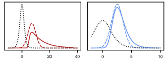
Second, the softmax-Dirichlet distribution is asymmetric for extremely sparse cases (see Figure 4). These arise in regions where the logistic transform (the 1D special case of the softmax) is nearly flat (as indicated by its derivative in Figure 4). Therefore, the LA is suboptimal in these high-variance cases.
This limitation can also be explained by looking at Equation (7). We observe that contributes linearly to with while contributes exponentially with . For settings where is small, this doesn’t have a large effect. However, when and grow the LB results differ from softmax Gaussian samples. In the LB, the resulting is dominated by the mean and the linear influence of the variance cannot correct sufficiently. For Monte Carlo sampling, on the other hand, the result is mostly determined by the large variance and then amplified through the softmax. Our proposed normalization to the LB reduces this effect (see Figure 3).
In BNNs, we often encounter such cases, especially far away from the data (see Figure 3 top). Therefore, we propose an additional correction for practical purposes:
| (12) | ||||
| (13) | ||||
| (14) |
where denotes the mean variance of , . The factor of is added because we found that higher dimensionalities require less correction. Since our correction is just a rescaling, the zero-sum constrained is still fulfilled. This normalization that can be understood as “pulling back” the distribution into a space where it is symmetric has higher approximation quality. This correction is applied after the zero-sum constraint correction.
We want to point out that our correction is motivated by experimentation and the theoretical insights detailed above. There is no theoretical derivation from first principles for the correction. We provide additional explanations and figures in Appendix A.
Throughout the paper, we will call this normalizing correction LB-norm and explicitly state when we use it. Otherwise, we will use the vanilla version with zero-sum correction.
5 Related Work
| Diag.-LA + MC | Diag.-LA + LB | Diag.-LA + LB-norm | Kron.-LA + MC | Kron.-LA + LB | Kron.-LA + LB-norm | ||||||||
| Train | Test | ECE | AUROC | ECE | AUROC | ECE | AUROC | ECE | AUROC | ECE | AUROC | ECE | AUROC |
| MNIST | FMNIST | 0.464 | 0.975 | 0.478 | 0.981 | 0.498 | 0.951 | 0.390 | 0.987 | 0.553 | 0.977 | 0.364 | 0.990 |
| MNIST | notMNIST | 0.396 | 0.965 | 0.600 | 0.930 | 0.360 | 0.955 | 0.366 | 0.974 | 0.634 | 0.912 | 0.294 | 0.986 |
| MNIST | KMNIST | 0.429 | 0.974 | 0.617 | 0.949 | 0.391 | 0.970 | 0.374 | 0.985 | 0.619 | 0.956 | 0.328 | 0.991 |
| CIFAR10 | CIFAR100 | 0.379 | 0.887 | 0.691 | 0.859 | 0.220 | 0.883 | 0.577 | 0.878 | 0.670 | 0.855 | 0.558 | 0.866 |
| CIFAR10 | SVHN | 0.309 | 0.948 | 0.652 | 0.928 | 0.155 | 0.948 | 0.447 | 0.955 | 0.635 | 0.924 | 0.327 | 0.965 |
| SVHN | CIFAR100 | 0.615 | 0.957 | 0.667 | 0.962 | 0.679 | 0.944 | 0.583 | 0.959 | 0.659 | 0.962 | 0.575 | 0.953 |
| SVHN | CIFAR10 | 0.600 | 0.958 | 0.659 | 0.960 | 0.662 | 0.947 | 0.567 | 0.960 | 0.651 | 0.959 | 0.556 | 0.955 |
| CIFAR100 | CIFAR10 | 0.474 | 0.788 | 0.239 | 0.791 | 0.834 | 0.757 | 0.479 | 0.787 | 0.202 | 0.790 | 0.855 | 0.749 |
| CIFAR100 | SVHN | 0.470 | 0.795 | 0.207 | 0.815 | 0.842 | 0.748 | 0.469 | 0.798 | 0.183 | 0.807 | 0.849 | 0.761 |
In BNNs, analytic approximations of posterior predictive distributions have attracted a great deal of research. In the binary classification case, for example, the probit approximation [Gibbs, 1997, Lu et al., 2020] has been proposed already in the 1990s [Spiegelhalter and Lauritzen, 1990, MacKay, 1992b]. However, while there exist some bounds [Titsias, 2016] and approximations of the expected log-sum-exponent function [Ahmed and Xing, 2007, Braun and McAuliffe, 2010], in the multi-class case, obtaining a good analytic approximation of the expected softmax function under a Gaussian measure is an open problem. Our LB can be used to produce a close analytical approximation of this integral. It thus furthers the trend of sampling-free solutions within Bayesian Deep Learning [Wu et al., 2018, Haussmann et al., 2019, etc.]. The crucial difference is that, unlike these methods, the LB approximates the full distribution over the softmax outputs of a deep network.
Previous approaches proposed to model the distribution of softmax outputs of a network directly. Similar to the LB, Malinin and Gales [2018, 2019], Sensoy et al. [2018] proposed to use the Dirichlet distribution to model the posterior predictive for non-Bayesian networks. They further proposed novel training techniques in order to directly learn the Dirichlet. Additionally, different work on Distillation [Malinin et al., 2019, Vadera et al., 2020] takes larger models and distills them into a smaller one. The result of some distillation methods is a Dirichlet similar to the LB. We compare against prior nets in the experiments.
In contrast, the LB tackles the problem of approximating the distribution over the softmax outputs of the ubiquitous Gaussian-approximated BNNs [Graves, 2011, Blundell et al., 2015, Louizos and Welling, 2016, Sun et al., 2017, etc] without any additional training procedure. Therefore the LB can, for example, be used with pre-trained weights on large datasets while prior networks and distillation usually require training from scratch.
6 Experiments
| Diag Probit | Diag LB norm | ||||||||||
| Train | Test | MMC | AUROC | NLL | ECE | Brier | MMC | AUROC | NLL | ECE | Brier |
| MNIST | MNIST | 0.967 | - | 0.050 | 0.024 | 0.002 | 0.944 | - | 0.078 | 0.045 | 0.003 |
| MNIST | FMNIST | 0.597 | 0.971 | 3.827 | 0.523 | 0.128 | 0.589 | 0.951 | 3.538 | 0.498 | 0.124 |
| MNIST | notMNIST | 0.616 | 0.958 | 3.839 | 0.488 | 0.123 | 0.492 | 0.955 | 3.070 | 0.360 | 0.111 |
| MNIST | KMNIST | 0.580 | 0.969 | 4.276 | 0.489 | 0.126 | 0.484 | 0.970 | 3.288 | 0.391 | 0.115 |
| CIFAR10 | CIFAR10 | 0.869 | - | 0.237 | 0.083 | 0.009 | 0.517 | - | 0.727 | 0.433 | 0.029 |
| CIFAR10 | CIFAR100 | 0.589 | 0.882 | 3.334 | 0.485 | 0.123 | 0.319 | 0.883 | 2.590 | 0.220 | 0.099 |
| CIFAR10 | SVHN | 0.510 | 0.946 | 3.097 | 0.394 | 0.114 | 0.273 | 0.948 | 2.457 | 0.155 | 0.094 |
| Diag.-LA + MC | Diag.-LA + LB | Diag.-LA + LB-norm | Kron.-LA + MC | Kron.-LA + LB | Kron.-LA + LB-norm | ||||||||
|---|---|---|---|---|---|---|---|---|---|---|---|---|---|
| Train | Test | ECE | AUROC | ECE | AUROC | ECE | AUROC | ECE | AUROC | ECE | AUROC | ECE | AUROC |
| MNIST | FMNIST | 0.464 | 0.975 | 0.478 | 0.981 | 0.498 | 0.951 | 0.390 | 0.987 | 0.553 | 0.977 | 0.364 | 0.990 |
| MNIST | notMNIST | 0.396 | 0.965 | 0.600 | 0.930 | 0.360 | 0.955 | 0.366 | 0.974 | 0.634 | 0.912 | 0.294 | 0.986 |
| MNIST | KMNIST | 0.429 | 0.974 | 0.617 | 0.949 | 0.391 | 0.970 | 0.374 | 0.985 | 0.619 | 0.956 | 0.328 | 0.991 |
| MNIST | FMNIST | 0.317 | 0.980 | 0.322 | 0.990 | 0.123 | 0.986 | 0.288 | 0.985 | 0.528 | 0.980 | 0.135 | 0.991 |
| MNIST | notMNIST | 0.280 | 0.960 | 0.566 | 0.924 | 0.126 | 0.952 | 0.282 | 0.958 | 0.629 | 0.915 | 0.171 | 0.973 |
| MNIST | KMNIST | 0.309 | 0.976 | 0.557 | 0.955 | 0.112 | 0.972 | 0.279 | 0.981 | 0.615 | 0.958 | 0.152 | 0.986 |
| Prior Network | Diag LB norm | ||||||||||
|---|---|---|---|---|---|---|---|---|---|---|---|
| Train | Test | MMC | AUROC | ECE | NLL | Brier | MMC | AUROC | ECE | NLL | Brier |
| MNIST | MNIST | 0.802 | - | 0.184 | 0.246 | 0.008 | 0.944 | - | 0.045 | 0.078 | 0.003 |
| MNIST | FMNIST | 0.273 | 0.995 | 0.212 | 2.659 | 0.098 | 0.589 | 0.951 | 0.498 | 3.538 | 0.124 |
| MNIST | notMNIST | 0.447 | 0.938 | 0.314 | 2.962 | 0.105 | 0.492 | 0.955 | 0.360 | 3.070 | 0.111 |
| MNIST | KMNIST | 0.372 | 0.976 | 0.261 | 3.142 | 0.104 | 0.484 | 0.970 | 0.391 | 3.288 | 0.115 |
We conduct multiple experiments. Firstly, we compare the LB to the MC-integral on a 2D toy example (Section 6.1). Secondly, we apply the same comparison to out-of-distribution (OOD) detection in many settings (Section 6.2). Thirdly, we compare the commonly used probit approximation to the LB in section 6.3 Fourthly, we compare their computational cost and contextualize the speed-up for the prediction process in Section 6.4. Finally, in Section 6.5, we present analysis on ImageNet [Russakovsky et al., 2014] to demonstrate the scalability of the LB and the advantage of having a full Dirichlet distribution over softmax outputs. We extended Laplace torch [Daxberger et al., 2021] for the experiments. Code can be found in the accompanying GitHub repository.222https://github.com/mariushobbhahn/LB_for_BNNs_official
For all experiments, a last-layer Laplace approximation has been applied. This scheme has been successfully used by Snoek et al. [2015], Kristiadi et al. [2020]. We use diagonal and Kronecker-factorized (KFAC)[Ritter et al., 2018, Martens and Grosse, 2015] approximations of the Hessian, since inverting the exact Hessian is too costly. A detailed mathematical explanation and setup of the experiments can be found in appendix D. While the LB could also be applied to different approximations of a Gaussian posterior predictive such as Variational Inference [Graves, 2011, Blundell et al., 2015], we used a Laplace approximation in our experiments to construct such an approximation. This is for two reasons: (i) it is one of the fastest ways to get a Gaussian posterior predictive and (ii) it can be applied to pre-trained networks which is especially useful for large problems such as ImageNet. Nevertheless, we want to emphasize again that the LB can be applied to any Gaussian over the outputs independent of the way it was generated.

6.1 2D Toy example
6.2 OOD detection
We compare the performance of the LB to the MC-integral (Diagonal and KFAC) on a standard OOD detection benchmark suite, to test whether the LB gives similar results to the MC sampling methods. Following prior literature, we use the standard expected calibration error (ECE) and area under the ROC-curve (AUROC) metrics [Hendrycks and Gimpel, 2016].
For the exact setup, we refer the reader to Appendix D. We use the mean of the Dirichlet to obtain a comparable approximation to the MC-integral. The results are presented in Table 1.
We find that the results of the LB or its normalized version are comparable throughout the entire benchmark suite. Since the LB is much faster it can be a good replacement for MC in time-sensitive applications.
Furthermore, we compare the LB to prior networks (PNs) in Table 4 since PNs also yield a Dirichlet distribution as an output on classification tasks. We find that PNs outperform the LB in most cases. However, we don’t think this is a major problem since they have different aims and use cases. The LB creates a Dirichlet distribution on top of an already existing Gaussian model while PNs describe a training procedure and have to be trained from scratch. Thus, the primary comparison for the LB should be against sampling and other integral approximations like in Table 2.
Lastly, we compare the LB for a full-layer vs. last-layer Laplace approximation of the network in Table 3. We find that, as expected, the full-layer setting yield slightly better results. However, since the primary advantage of the LB is its speed, we think the natural fit for it is a last-layer approximation.
| # samples in brackets | Forward pass | MC(1000) | MC(100) | MC(10) | Laplace Bridge |
|---|---|---|---|---|---|
| Time in seconds | 0.300 0.003 | 4.712 0.063 | 0.488 0.009 | 0.059 0.001 | 0.013 0.000 |
| Fraction of overall time | 0.06/0.38/0.83/0.96 | 0.94 | 0.62 | 0.17 | 0.04 |

6.3 Comparison to the probit approximation
The multi-class probit approximation [Gibbs, 1997, Lu et al., 2020] is a commonly used approximation for the softmax-Gaussian integral. We compare it to the diagonal normalized LB in Table 2. We find that the LB norm outperforms the probit approximation in most OOD tasks. When we use a KFAC approximation of the Hessian, this trend still holds (see Table 6 in Appendix D).
6.4 Time comparison
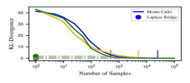
We compare the computational cost of the density-estimated distribution via sampling and the Dirichlet obtained from the LB for approximating the true over MC-sampling. Different numbers of samples are drawn from the Gaussian, the softmax is applied and the KL-divergence between the histogram of the samples with the true distribution is computed. We use KL-divergences and , respectively, to measure similarity between approximations and ground truth while the number of samples for is increased exponentially. The true distribution is constructed via MC with k samples. The experiment is conducted for three different Gaussian distributions over . Since the softmax applied to a Gaussian does not have an analytic form, the algebraic calculation of the approximation error is not possible and an empirical evaluation via sampling is the best option. The fact that there is no analytic solution is part of the justification for using the LB in the first place.
Figure 5 suggests that the number of samples required such that the distribution approximates the true distribution as good as the Dirichlet distribution obtained via the LB is large, i.e. somewhere between and k. This translates to a wall-clock time advantage of at least a factor of before sampling becomes competitive in quality with the LB.
To further demonstrate the low compute cost of the LB, we timed different parts of the process for our setup. On our hardware and setup, training a ResNet-18 on CIFAR10 over 130 epochs takes 71 minutes and 30 seconds. Computing a Hessian for the network from the training data can be done with BackPACK [Dangel et al., 2020] at the cost of one backward pass over the training data or around 29 seconds. This one additional backward pass is the only change to the training procedure compared to conventional training. Since the LB only applies to the last step of the prediction pipeline, it is important to compare it to a forward pass through the rest of the network. Re-using the ResNet-18 and CIFAR10 setup we measure the time in seconds for a forward pass, for the application of the LB, and for the sampling procedure with 10, 100, and 1000 samples. The resulting sum total time for the entire test set is given in Table 5. We find that sampling takes up between 94% (for 1000 samples) and 17% (for 10 samples) of the entire prediction while the LB is only 4%. Thus, the acceleration through the LB is a significant improvement for the prediction process as a whole, not only for a part of the pipeline.
6.5 Uncertainty-aware output ranking on ImageNet
Due to the cost of sampling-based inference, classification on large datasets with many classes, like ImageNet, is rarely done in a Bayesian fashion. Instead, models for such tasks are often compared along a top- metric (e.g. ).
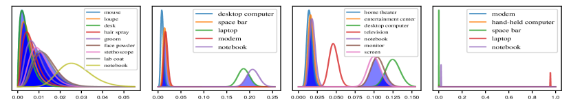
Although widely accepted, this metric has some pathologies: Depending on how close the point predictions are relative to their uncertainty, the total number of likely class labels should be allowed to vary from case to case. Figure 6 shows examples: In some cases (panel 2) the classifier is quite confident that the image in question belongs to one out of only two classes and all others are highly unlikely. In others (e.g. panel 1), a larger set of hypotheses are all nearly equally probable.
The Laplace Bridge, in conjunction with the last-layer Laplace approximations, can be used to address this issue. To this end, the analytic properties of its Dirichlet prediction are particularly useful: Recall that the marginal distribution over each component of a Dirichlet relative to all other components is .
We leverage this property to propose a simple uncertainty-aware top- decision rule inspired by statistical tests. Instead of keeping fixed, it uses the model’s confidence to adapt (pseudo-code in Algorithm 1).
We begin by sorting the class predictions in order of their expected probability . Then we compute the Beta marginal of the most likely class. Now, we compute the overlap of the next marginal and add that class to the list iff the overlap is more than some threshold (e.g. 0.05). Continuing in this fashion, the algorithm terminates with a finite value of “non-separated” top classes.
The intuition behind this rule is that, if any Beta density overlaps with the most likely one more than the threshold of, say, , the classifier cannot confidently predict one class over the other. Thus, all classes sufficiently overlapping with the top contender should be returned as the top estimates.


We evaluate this decision rule on the test set of ImageNet. The overlap is calculated through the inverse CDF333Also known as the quantile function or percent point function of the respective Beta marginals. The original top- accuracy of DenseNet on ImageNet is . In contrast, the uncertainty-aware top-k method yields accuracies of over while average list lengths stay below (see Figure 7). Furthermore, we find that most of the predictions given by the uncertainty-aware metric still yielded a top- prediction. This means that using uncertainty does not imply adding meaningless classes to the prediction. Furthermore, there are non-negligibly many cases where equals to , , or (all values larger than are in the bin).
Thus, using the uncertainty-aware prediction rule above, the classifier can use its uncertainty to adaptively return a longer or shorter list of predictions. This not only allows it to improve accuracy over a hard top-1 threshold. Arguably, the ability to vary the size of the predicted set of classes is a practically useful functionality in itself. As Figure 6 shows anecdotally, some of the labels (like “notebook” and “laptop”) are semantically so similar to each other that it would seem only natural for the classifier to use them synonymously.
7 Conclusion
We have adapted a previously developed approximation scheme for new use in Bayesian Deep Learning. Given a Gaussian approximation to the weight-space posterior of a NN (which can be constructed by various means, including another Laplace approximation), and an input, the Laplace Bridge analytically maps the marginal Gaussian prediction on the logits onto a Dirichlet distribution over the softmax vectors. The associated computational cost of for -class prediction compares favorably to that of MC sampling. The proposed method empirically preserves predictive uncertainty, offering an attractive, low-cost, high-quality alternative to Monte Carlo sampling. In conjunction with a low-cost, last-layer Bayesian approximation, it is useful in real-time applications wherever uncertainty is required—especially because it drastically reduces the cost of predicting a posterior distribution at test time for a minimal increase in cost at training time. The vanilla LB has some limitations, for which we proposed a simple correction that outperforms alternative softmax-integral approximations such as the commonly used multi-class probit. We demonstrate the utility of the scheme for large-scale Bayesian inference by using it to construct an uncertainty-aware top- ranking on ImageNet.
MH wrote the code, created the figures, and wrote most of the paper. AK gave guidance and supervision and assisted throughout the entire process and greatly helped with the rebuttal. PH had the original idea and provided supervision.
Acknowledgements.
The authors gratefully acknowledge financial support by the European Research Council through ERC StG Action 757275 / PANAMA; the DFG Cluster of Excellence “Machine Learning - New Perspectives for Science”, EXC 2064/1, project number 390727645; the German Federal Ministry of Education and Research (BMBF) through the Tübingen AI Center (FKZ: 01IS18039A); and funds from the Ministry of Science, Research and Arts of the State of Baden-Württemberg. MH & AK are grateful to Alexander Meinke for the pre-trained models and the International Max Planck Research School for Intelligent Systems (IMPRS-IS) for support. MH & AK would also like to thank all members of Methods of Machine Learning group for helpful feedback.References
- Ahmed and Xing [2007] Amr Ahmed and Eric Xing. On tight approximate inference of the logistic-Normal topic admixture model. In Proceedings of the 11th Tenth International Workshop on Artificial Intelligence and Statistics, 2007.
- Begoli et al. [2019] E. Begoli, T. Bhattacharya, and D. Kusnezov. The need for uncertainty quantification in machine-assisted medical decision making. Nat Mach Intell, 1:20–23, 2019.
- Blundell et al. [2015] Charles Blundell, Julien Cornebise, Koray Kavukcuoglu, and Daan Wierstra. Weight uncertainty in neural network. In ICML, pages 1613–1622. PMLR, 2015.
- Braun and McAuliffe [2010] Michael Braun and Jon McAuliffe. Variational inference for large-scale models of discrete choice. Journal of the American Statistical Association, 105(489):324–335, 2010.
- Brosse et al. [2020] Nicolas Brosse, Carlos Riquelme, Alice Martin, Sylvain Gelly, and Éric Moulines. On last-layer algorithms for classification: Decoupling representation from uncertainty estimation. arXiv preprint arXiv:2001.08049, 2020.
- Bulatov [2011] Yaroslav Bulatov. notMNIST dataset, 2011. URL http://yaroslavvb.blogspot.com/2011/09/notmnist-dataset.html.
- Clanuwat et al. [2018] Tarin Clanuwat, Mikel Bober-Irizar, Asanobu Kitamoto, Alex Lamb, Kazuaki Yamamoto, and David Ha. Deep learning for classical Japanese literature. arXiv, abs/1812.01718, 2018.
- Dangel et al. [2020] Felix Dangel, Frederik Kunstner, and Philipp Hennig. Backpack: Packing more into backprop. In International Conference on Learning Representations, 2020.
- Daxberger et al. [2021] Erik Daxberger, Agustinus Kristiadi, Alexander Immer, Runa Eschenhagen, Matthias Bauer, and Philipp Hennig. Laplace redux–effortless Bayesian deep learning. In NeurIPS, 2021.
- Gibbs [1997] Mark N. Gibbs. Bayesian Gaussian Processes for Regression and Classification. PhD thesis, University of Cambridge, September 1997.
- Graves [2011] Alex Graves. Practical Variational Inference for neural networks. In J. Shawe-Taylor, R. S. Zemel, P. L. Bartlett, F. Pereira, and K. Q. Weinberger, editors, Advances in Neural Information Processing Systems 24, pages 2348–2356. Curran Associates, Inc., 2011.
- Haussmann et al. [2019] Manuel Haussmann, Sebastian Gerwinn, and Melih Kandemir. Bayesian evidential deep learning with pac regularization, 2019.
- He et al. [2016] Kaiming He, Xiangyu Zhang, Shaoqing Ren, and Jian Sun. Deep residual learning for image recognition. In Proceedings of the IEEE conference on computer vision and pattern recognition, pages 770–778, 2016.
- Hein et al. [2019] Matthias Hein, Maksym Andriushchenko, and Julian Bitterwolf. Why relu networks yield high-confidence predictions far away from the training data and how to mitigate the problem. In The IEEE Conference on Computer Vision and Pattern Recognition (CVPR), June 2019.
- Hendrycks and Gimpel [2016] Dan Hendrycks and Kevin Gimpel. A baseline for detecting misclassified and out-of-distribution examples in neural networks. arXiv, abs/1610.02136, 2016.
- Hennig [2010] P. Hennig. Approximate Inference in Graphical Models. PhD thesis, University of Cambridge, November 2010.
- Hennig et al. [2012] P. Hennig, D. Stern, R. Herbrich, and T. Graepel. Kernel topic models. In Fifteenth International Conference on Artificial Intelligence and Statistics, volume 22 of JMLR Proceedings, pages 511–519. JMLR.org, 2012.
- Kristiadi et al. [2020] Agustinus Kristiadi, Matthias Hein, and Philipp Hennig. Being Bayesian, even just a bit, fixes overconfidence in relu networks. In ICML, pages 5436–5446. PMLR, 2020.
- Krizhevsky et al. [2014] Alex Krizhevsky, Vinod Nair, and Geoffrey Hinton. The CIFAR-10 dataset. online: http://www. cs. toronto. edu/kriz/cifar. html, 55, 2014.
- LeCun [1998] Y. LeCun. The MNIST database of handwritten digits. http://yann.lecun.com/exdb/mnist/, 1998.
- Louizos and Welling [2016] Christos Louizos and Max Welling. Structured and efficient Variational deep learning with matrix Gaussian posteriors. In ICML, 2016.
- Lu et al. [2020] Zhiyun Lu, Eugene Ie, and Fei Sha. Uncertainty estimation with infinitesimal jackknife, its distribution and mean-field approximation. CoRR, abs/2006.07584, 2020. URL https://arxiv.org/abs/2006.07584.
- MacKay [1992a] David J. C. MacKay. A practical Bayesian framework for backpropagation networks. Neural Comput., 4(3):448–472, May 1992a. ISSN 0899-7667.
- Mackay [1995] David J C Mackay. Probable networks and plausible predictions — a review of practical Bayesian methods for supervised neural networks. Network: Computation in Neural Systems, 6(3):469–505, 1995.
- MacKay [1992b] David JC MacKay. The evidence framework applied to classification networks. Neural computation, 4(5):720–736, 1992b.
- MacKay [1998] David J.C. MacKay. Choice of basis for laplace approximation. Machine Learning, 33(1):77–86, Oct 1998. ISSN 1573-0565.
- Malinin and Gales [2018] Andrey Malinin and Mark Gales. Predictive uncertainty estimation via prior networks. In Advances in Neural Information Processing Systems, pages 7047–7058, 2018.
- Malinin and Gales [2019] Andrey Malinin and Mark Gales. Reverse KL-divergence training of prior networks: Improved uncertainty and adversarial robustness. In Advances in Neural Information Processing Systems, pages 14520–14531, 2019.
- Malinin et al. [2019] Andrey Malinin, Bruno Mlodozeniec, and Mark Gales. Ensemble distribution distillation, 2019.
- Martens and Grosse [2015] James Martens and Roger Grosse. Optimizing neural networks with Kronecker-factored approximate curvature. In ICML, 2015.
- McAllister et al. [2017] Rowan McAllister, Yarin Gal, Alex Kendall, Mark van der Wilk, Amar Shah, Roberto Cipolla, and Adrian Weller. Concrete problems for autonomous vehicle safety: Advantages of Bayesian deep learning. In IJCAI, 2017.
- Michelmore et al. [2018] Rhiannon Michelmore, Marta Kwiatkowska, and Yarin Gal. Evaluating uncertainty quantification in end-to-end autonomous driving control. CoRR, abs/1811.06817, 2018.
- Netzer et al. [2011] Yuval Netzer, Tao Wang, Adam Coates, Alessandro Bissacco, Bo Wu, and Andrew Y. Ng. Reading digits in natural images with unsupervised feature learning. In NIPS Workshop on Deep Learning and Unsupervised Feature Learning 2011, 2011.
- Nguyen et al. [2015] Anh Nguyen, Jason Yosinski, and Jeff Clune. Deep neural networks are easily fooled: High confidence predictions for unrecognizable images. In CVPR, 2015.
- Pedregosa et al. [2011] F. Pedregosa, G. Varoquaux, A. Gramfort, V. Michel, B. Thirion, O. Grisel, M. Blondel, P. Prettenhofer, R. Weiss, V. Dubourg, J. Vanderplas, A. Passos, D. Cournapeau, M. Brucher, M. Perrot, and E. Duchesnay. Scikit-learn: Machine learning in Python. Journal of Machine Learning Research, 12:2825–2830, 2011.
- Ritter et al. [2018] Hippolyt Ritter, Aleksandar Botev, and David Barber. A scalable laplace approximation for neural networks. In International Conference on Learning Representations, 2018.
- Russakovsky et al. [2014] Olga Russakovsky, Jia Deng, Hao Su, Jonathan Krause, Sanjeev Satheesh, Sean Ma, Zhiheng Huang, Andrej Karpathy, Aditya Khosla, Michael S. Bernstein, Alexander C. Berg, and Fei-Fei Li. Imagenet large scale visual recognition challenge. CoRR, abs/1409.0575, 2014.
- Sensoy et al. [2018] Murat Sensoy, Lance Kaplan, and Melih Kandemir. Evidential deep learning to quantify classification uncertainty. In Advances in Neural Information Processing Systems, pages 3179–3189, 2018.
- Snoek et al. [2015] Jasper Snoek, Oren Rippel, Kevin Swersky, Ryan Kiros, Nadathur Satish, Narayanan Sundaram, Mostofa Patwary, Mr Prabhat, and Ryan Adams. Scalable Bayesian optimization using deep neural networks. In Francis Bach and David Blei, editors, Proceedings of the 32nd ICML, volume 37 of Proceedings of Machine Learning Research, pages 2171–2180, Lille, France, 07–09 Jul 2015. PMLR.
- Spiegelhalter and Lauritzen [1990] David J Spiegelhalter and Steffen L Lauritzen. Sequential updating of conditional probabilities on directed graphical structures. Networks, 20(5):579–605, 1990.
- Sun et al. [2017] Shengyang Sun, Changyou Chen, and Lawrence Carin. Learning structured weight uncertainty in Bayesian neural networks. In Artificial Intelligence and Statistics, pages 1283–1292, 2017.
- Titsias [2016] Michalis Titsias. One-vs-each approximation to softmax for scalable estimation of probabilities. In NIPS, 2016.
- Vadera et al. [2020] Meet P. Vadera, Brian Jalaian, and Benjamin M. Marlin. Generalized bayesian posterior expectation distillation for deep neural networks, 2020.
- Wilson et al. [2016] Andrew Gordon Wilson, Zhiting Hu, Ruslan Salakhutdinov, and Eric P. Xing. Deep kernel learning. In Arthur Gretton and Christian C. Robert, editors, Proceedings of the 19th International Conference on Artificial Intelligence and Statistics, volume 51 of Proceedings of Machine Learning Research, pages 370–378, Cadiz, Spain, 09–11 May 2016. PMLR.
- Wu et al. [2018] Anqi Wu, Sebastian Nowozin, Edward Meeds, Richard E. Turner, José Miguel Hernández-Lobato, and Alexander L. Gaunt. Fixing Variational Bayes: Deterministic Variational Inference for Bayesian neural networks. arXiv, abs/1810.03958, 2018.
- Xiao et al. [2017] Han Xiao, Kashif Rasul, and Roland Vollgraf. Fashion-MNIST: a novel image dataset for benchmarking machine learning algorithms. arXiv, abs/1708.07747, 2017.
Appendix A Appendix
Figures
The parameters of Figure 2 are from left to right .
Change of Variable for pdf
Let be an -dimensional continuous random variable with joint density function . If , where is a differentiable function, then has density :
| (15) |
where the differential is the Jacobian of the inverse of evaluated at . This procedure, also known as ‘change of basis’, is at the core of the Laplace bridge since it is used to transform the Dirichlet into the softmax basis.
Correction for sum(y)=0
We know that the product rule of Gaussians yields
| (16) | ||||
| (17) | ||||
In our particular setup we have
| (18) |
with constraint
| (19) |
Therefore we get
| (20) | ||||
| (21) |
Variance correction
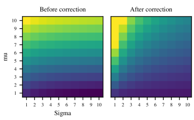
As described in the main text, the original Laplace Bridge scales worse with than sampling and applying the softmax. In Figure 8 you can see a contourplot that shows the scaling of mean and variance with and without correction. As suggested, the Variance has nearly no influence on the result before the correction but our correction fixes that.
Some reviewers wanted to understand how we derived the equations for our correction, so here is a short informal explanation. During the experimentation with the LB, we found that it doesn’t approximate the sample distribution well when gets large. We then understood why (as detailed in the limitations section) and proposed a fix for these scenarios without damaging its behavior in all other scenarios. We experimented with multiple fixes and the result you see in the paper is the one that fulfilled most of our criteria. Therefore, the correction doesn’t come from a principled theoretical derivation but is motivated by the theoretical findings.
Appendix B Appendix (Derivation of LB)
Assume we have a Dirichlet in the standard basis with parameter vector and probability density function:
| (22) |
We aim to transform the basis of this distribution via the softmax transform to be in the new base :
| (23) |
Usually, to transform the basis we would need the inverse transformation as described in the main paper. However, the softmax does not have an analytic inverse. Therefore David JC MacKay uses the following trick. Assume we know that the distribution in the transformed basis is:
| (24) |
then we can show that the original distribution is the result of the basis transform by the softmax.
The Dirichlet in the softmax basis: We show that the density over shown in Equation 24 transforms into the Dirichlet over . First, we consider the special case where is confined to an dimensional subspace satisfying . In this subspace we can represent by an dimensional vector such that
| (25) | ||||
| (26) |
and similarly we can represent by an dimensional vector :
| (27) | ||||
| (28) |
then we can find the density over (which is proportional to the required density over ) from the density over (which is proportional to the given density over ) by finding the determinant of the Jacobian given by
| (29) |
We define two additional dimensional helper vectors and , and use from linear algebra. It follows that
| (30) | ||||
Therefore, using Equation 24 we find that
| (31) |
This result is true for any constant since it can be put into the normalizing constant. Thereby we make sure that the integral of the distribution is 1 and we have a valid probability distribution.
Appendix C Appendix (Derivation of Inversion)
Through the figures of the 1D Dirichlet approximation in the main paper we have already established that the mode of the Dirichlet lies at the mean of the Gaussian distribution and therefore . Additionally, the elements of must sum to zero. These two constraints combined yield only one possible solution for .
| (32) |
Calculating the covariance matrix is more complicated but layed out in the following. The logarithm of the Dirichlet is, up to additive constants
| (33) |
Using as the softmax of as shown in Equation 23 we can find the elements of the Hessian
| (34) |
where and for the value of at the mode. Analytically inverting is done via a lengthy derivation using the fact that we can write and inverting it with the Schur-complement. You can find the derivation in [Hennig, 2010]. This process results in the inverse of the Hessian
| (35) |
We are mostly interested in the diagonal elements, since we desire a sparse encoding for computational reasons and we otherwise needed to map a covariance matrix to a Dirichlet parameter vector which would be a very overdetermined mapping. Note that is a scalar not a matrix. The diagonal elements of can be calculated as
| (36) |
To invert this mapping we transform Equation 32 to
| (37) |
by applying the logarithm and re-ordering some parts. Inserting this into Equation 36 and re-arranging yields
| (38) |
which can be re-inserted into Equation 37 to give
| (39) |
Appendix D Appendix (Experimental Details)
| KFAC Probit | KFAC LB norm | ||||||||
| Train | Test | MMC | AUROC | ECE | NLL | MMC | AUROC | ECE | NLL |
| MNIST | MNIST | 0.105 | 0.000 | 2.258 | 0.883 | 0.975 | 0.000 | 0.043 | 0.018 |
| MNIST | FMNIST | 0.102 | 0.955 | 2.302 | 0.032 | 0.444 | 0.990 | 2.871 | 0.364 |
| MNIST | notMNIST | 0.103 | 0.922 | 2.300 | 0.043 | 0.409 | 0.986 | 2.854 | 0.294 |
| MNIST | KMNIST | 0.102 | 0.962 | 2.304 | 0.012 | 0.414 | 0.991 | 3.162 | 0.328 |
| CIFAR10 | CIFAR10 | 0.548 | 0.000 | 0.661 | 0.404 | 0.941 | 0.000 | 0.195 | 0.017 |
| CIFAR10 | CIFAR100 | 0.358 | 0.896 | 2.652 | 0.253 | 0.662 | 0.866 | 3.871 | 0.558 |
| CIFAR10 | SVHN | 0.307 | 0.956 | 2.567 | 0.195 | 0.441 | 0.965 | 2.837 | 0.327 |
The exact experimental setups, i.e. network architectures, learning rates, random seeds, etc. can be found in the accompanying GitHub repository 444https://github.com/mariushobbhahn/LB_for_BNNs_official. This section is used to justify some of the decisions we made during the process in more detail, highlight some miscellaneous interesting things and showcase the additional experiments promised in the main paper.
Mathematical description of the setup
In principle, the Gaussian over the weights required by the Laplace Bridge for BNNs can be constructed by any Gaussian approximate Bayesian method such as variational Bayes [Graves, 2011, Blundell et al., 2015] and Laplace approximations for NNs [MacKay, 1992a, Ritter et al., 2018]. We will focus on the Laplace approximation, which uses the same principle as the Laplace Bridge. However, in the Laplace approximation for neural networks, the posterior distribution over the weights of a network is the one that is approximated as a Gaussian, instead of a Dirichlet distribution over the outputs as in the Laplace Bridge.
Given a dataset and a prior , let
| (40) |
be the posterior over the parameter of an -layer network . Then we can get an approximation of the posterior by fitting a Gaussian where
That is, we fit a Gaussian centered at the mode of with the covariance determined by the curvature at that point. We assume that the prior is a zero-mean isotropic Gaussian and the likelihood function is the Categorical density
For various applications in Deep Learning, an approximation with full Hessian is often computationally too expensive. Indeed, for each input , one has to do backward passes to compute the Jacobian . Moreover, it requires an storage which is also expensive since is often in the order of millions. A cheaper alternative is to fix all but the last layer of and only apply the Laplace approximation on , the last layer’s weight matrix. This scheme has been used successfully by Snoek et al. [2015], Wilson et al. [2016], Brosse et al. [2020], etc. and has been shown theoretically that it can mitigate overconfidence problems in ReLU networks [Kristiadi et al., 2020]. In this case, given the approximate last-layer posterior
| (41) |
one can efficiently compute the distribution over the logits. That is, let be the first layers of , seen as a feature map. Then, for each , the induced distribution over the logit is given by
| (42) |
where denotes the Kronecker product.
An even more efficient last-layer approximation can be obtained using a Kronecker-factored matrix normal distribution [Louizos and Welling, 2016, Sun et al., 2017, Ritter et al., 2018]. That is, we assume the posterior distribution to be
| (43) |
where and are the Kronecker factorization of the inverse Hessian matrix [Martens and Grosse, 2015] and denotes the Matrix Normal distribution. In this case, for any , one can easily show that the distribution over logits is given by
| (44) |
which is easy to implement and computationally cheap. Finally, and even more efficient, is a last-layer approximation scheme with a diagonal Gaussian approximate posterior, i.e. the so-called mean-field approximation. In this case, we assume the posterior distribution to be
| (45) |
where is obtained via the diagonal of the Hessian of the log-posterior w.r.t. at .
OOD Detection
The test scenarios are: A two-layer convolutional network trained on the MNIST dataset [LeCun, 1998]. The OOD datasets for this case are FMNIST [Xiao et al., 2017], notMNIST [Bulatov, 2011], and KMNIST [Clanuwat et al., 2018]. For larger datasets, i.e. CIFAR-10 [Krizhevsky et al., 2014], SVHN [Netzer et al., 2011], and CIFAR-100 [Krizhevsky et al., 2014], we use a ResNet-18 network [He et al., 2016]. In all scenarios, the networks are well-trained with test accuracy on MNIST, on CIFAR-10, on CIFAR-100, and on SVHN. For the sampling baseline, we use posterior samples.
All network have been trained with conventional setups, i.e. we use ADAM with learning rate and weight decay for the MNIST experiments and SGD with a cosine annealing scheduler starting at learning rate and momentum for the CIFAR and SVHN experiments.
Probit vs LB
The KFAC setting of the probit comparison can be found in Table 6. Especially in the MNIST scenario the probit approximation seems to break down since even in-dist detection is at chance level. The LB, on the other hand, yields reasonable results.