A Correlation Method for Deriving UA Intra-Molecular Potentials from AA Molecular Dynamics Simulations: Application to Alkanes

Abstract

Unified-Atom (UA) force fields are usually constructed using a Boltzmann-inverse method based on distributions obtained from Monte-Carlo simulations. A new method of constructing UA force fields from All-Atom (AA) molecular dynamics simulations is proposed. In this method, one determines time correlations between oscillators of the same type: between a CC bond and the connected CH bonds; between a valence angle CCC and all valence angles sharing at least one hydrogen with it; between a dihedral angle CCCC and the dihedral angles sharing the two central carbons with it. In the case of no correlation between lengths or angles, energies of the oscillators are independent. In this case, the AA and UA components of the force fields are identical. When a correlation is total, the UA potential of an object is the sum of the energies of the oscillators coupled to it. Partial correlations are also possible. Several kinematic matching tests of the AA molecule with the corresponding UA molecule are considered: mean periods of vibration of the oscillators; energies associated with presence probabilities; mean end-to-end lengths of the molecules. The method is, as an example, applied to aliphatic molecules, simulated with the OPLS-AA force field.

Keywords.

Molecular Dynamics ; Potential ; All-Atom ; United-Atom ; Correlation method ; OPLS ; Alkane

1 Introduction

Molecular Dynamics [1] (MD) simulations at the All-Atom (AA) level are a recognized technique for predicting the behaviour of molecules at the atomic scale. The time scale is limited by a time-step of no more than 1 femto-second (${1}\>\mathit{fs}$) for molecules with CH bonds ($\approx{10}\>\mathit{fs}$). Thus, an AA simulation up to one nano-second (${1}\>\mathit{ns}$) requires at least $10^{6}$ time-steps. A large number of simulations, dealing for example with diffusion phenomena, require longer times.

Incorporating hydrogen atoms into grains is the standard technique for bypassing the time limitation associated with the time-step. This approach, called Unified-Atom (UA), also reduces the number of degrees of freedom and, therefore, the complexity of the models. In an UA hydrocarbon chain, for example, each grain is composed of one carbon atom and two or three hydrogen atoms (three hydrogens at both ends of the chain) and the mass of a grain is the sum of the mass of all the atoms it contains. The UA level is actually the first step of the Coarse-Grained (CG) approach in which grains can have more complex structures.

UA simulations should have kinematics and dynamics as close as possible to those in AA, under the same conditions. This proximity must exist both locally, at the level of each oscillator, and globally, with regard to the conformation of the molecule. As the kinematics and dynamics of the molecules depend on the potentials, these must be coherent at the AA and UA scales.

AA atoms and UA grains are structured within molecules by bonds, valence angles and dihedral angles which are oscillators whose behaviors are specified by their potentials grouped in force fields. To the intra-molecular potentials of the force fields are added inter-molecular potentials, corresponding to van der Waals interactions. The AA force field that will be considered in this text is OPLS-AA [4]. In this one, the potentials of the bonds and of the valence angles are harmonic functions, those of the dihedral angles are triple-cosine functions, and the inter-molecular potentials are Lennard-Jones 6-12 functions.

Most of the UA force fields are determined using Monte-Carlo simulations performed on dense matter at AA level [6, 5, 8, 7, 9, 14, 12, 13]. They are extracted from the simulation data using a Boltzmann-inverse approach, providing energies from the probabilities of presence of the simulation (micro-)states. These determinations are centered on dihedral angle potentials and inter-molecular potentials. Bond potentials and valence angle potentials are generally defined, without any particular justification, as being the same as in AA.

It is recognised that the terms of intra-molecular potential energy are much more important than those of inter-molecular interaction energy [15]. In a crystal, in particular, the equilibrium conformation of an isolated molecule is only slightly modified by inter-molecular interactions [10] and thus depends mainly on intra-molecular components. In this paper, only the intra-molecular components of the OPLS-UA force field [9] are considered.

In the proposed approach, intra-molecular UA potentials are defined from simulations of individual AA molecules, in the vacuum and at different temperatures. Each oscillator (bond, valence angle, dihedral angle) is studied individually. This study is based on the determination of temporal correlations between oscillators of the same type and the UA potentials are deduced from the correlations found.

2 Correlation Method

The correlation method is a general method, to deduce a UA potential using data from Molecular Dynamics AA simulations. It is presented here in the framework of alkanes which are linear (aliphatic) hydrocarbon chains. To simplify the analysis, only fragments of molecules will be considered in which each carbon always has two associated hydrogens (and not three for the extreme carbons). Thus, the fragments considered will always have a structure of the form ${C_{\mathit{n}}H_{\mathit{2n}}}$. At the UA level, fragments are chains of grains $G_{n}$. A natural correspondence exists between the AA fragment ${C_{\mathit{n}}H_{\mathit{2n}}}$ and the UA fragment $G_{n}$ which associates the grain $G_{i}$ to the carbon $C_{i}$ and to its two linked hydrogens (the center of the UA grain being the carbon atom).

We number the atoms in the ${C_{\mathit{N}}H_{\mathit{2N}}}$ fragment in the following way: the carbons are numbered consecutively, from 0 to $\mathit{N-1}$ and the two carbon-bonded hydrogens $C_{n}$ are numbered $\mathit{N+2n}$ and $\mathit{N+2n+1}$. Figure 1 shows the numbering of the atoms of fragment ${C_{\mathit{6}}H_{\mathit{12}}}$ as well as that of the grains of the corresponding fragment $G_{6}$. In the following, to simplify, we will no longer speak of fragment but only of a molecule.

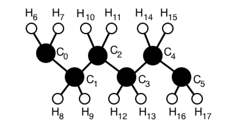
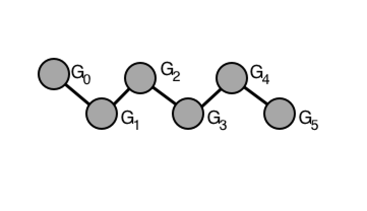
Figure 1: Left Image: Numbering of alkane fragment ${C_{\mathit{6}}H_{\mathit{12}}}$ atoms. Right Image: UA corresponding fragment $G_{6}$.

The temporal correlation method analyses the average evolution of an oscillator of the carbon chain according to those of the hydrocarbon oscillators of the same type (bond, valence angle or dihedral angle) that are coupled to it. Three types of couplings are defined:

• Couplings between CC and CH bonds. The CH bonds coupled to the bond ${C_{i}C_{i+1}}$ in the molecule ${C_{\mathit{n}}H_{\mathit{2n}}}$ are the 4 bonds ${C_{i}H_{n+2i}}$, ${C_{i}H_{n+2i+1}}$, ${C_{i+1}H_{n+2i+2}}$ and ${C_{i+1}H_{n+2i+3}}$.

• Couplings between CCC valence angles and valence angles CCH or HCH. The CCH angles coupled to the ${C_{i}C_{i+1}C_{i+2}}$ angle in the molecule ${C_{\mathit{n}}H_{\mathit{2n}}}$ are the four angles ${H_{n+2i}C_{i}C_{i+1}}$, ${H_{n+2i+1}C_{i}C_{i+1}}$, ${H_{i+1}C_{i+2}C_{n+2i+4}}$ and ${C_{i+1}C_{i+2}H_{n+2i+5}}$. The only HCH angle coupled with ${C_{i}C_{i+1}C_{i+2}}$ is the angle ${H_{n+2i+2}C_{i+1}H_{n+2i+3}}$.

• Couplings between CCCC dihedral angles and dihedral angles CCCH or HCCH. The HCCH angles coupled to ${C_{i}C_{i+1}C_{i+2}C_{i+3}}$ in the molecule ${C_{\mathit{n}}H_{\mathit{2n}}}$ are the four dihedral angles ${H_{n+2i+2}C_{i+1}C_{i+2}H_{n+2i+4}}$, ${H_{n+2i+3}C_{i+1}C_{i+2}H_{n+2i+4}}$, ${H_{n+2i+2}C_{i+1}C_{i+2}H_{n+2i+5}}$ and ${H_{n+2i+3}C_{i+1}C_{i+2}H_{n+2i+5}}$. The CCCH angles coupled with ${C_{i}C_{i+1}C_{i+2}C_{i+3}}$ in the molecule ${C_{\mathit{n}}H_{\mathit{2n}}}$ are the four angles ${H_{n+2i+2}C_{i+1}C_{i+2}C_{i+3}}$, ${H_{n+2i+3}C_{i+1}C_{i+2}C_{i+3}}$, ${H_{i}C_{i+1}C_{i+2}C_{n+2i+4}}$ as well as the angle ${C_{i}C_{i+1}C_{i+2}H_{n+2i+5}}$.

Molecular dynamics providing the coordinates of all atoms at each time-step, one can measure the length of the bonds and the angular value of the valence angles and of the dihedral angles.

For each pair of coupled oscillators, the pairs formed by the values of the hydrocarbon oscillator and those of the carbonated oscillator, are measured at the same time, form a cloud of points. This cloud results from the fluctuation over time of the exchanges of kinetic energy between the two oscillators. We analyze the statistical dependence between pairs of values by means of a linear regression using a least square method that allows to get a correlation factor. There are three possible scenarios, with different consequences for the determination of the UA potential:

• The slope of the linear regression line is zero. This means that there is no temporal correlation between the value of the of the carbonated oscillator and that of the hydrocarbon oscillator. The carbonated oscillator thus evolves on average independently from the hydrocarbon oscillator. In the absence of correlation, the vibration of an AA component does not depend on those of the coupled oscillators. The potential energy of the UA component therefore does not include any energy contribution from hydrocarbon coupled oscillators. The UA component behaving in the same way as the corresponding AA carboned component, they must have the same potential.

• The correlation factor is equal to $-1$ or $1$. The points are distributed on either side of the mean regression line, due to the exchange of kinetic energy between these oscillators. The correlation is then perfect and the values of the hydrocarbon oscillator are in mean directly related to those of the carbonated oscillator. Therefore, the potential energy of the corresponding UA component must be the sum of the potential energy of the AA carbonated component, and of the potential energies of the hydrocarbon coupled oscillators.

• The correlation factor is between $-1$ and $1$ and is different from $0$. Such a case is characteristic of a correlation between the hydrocarbon oscillators and the carbonated component. In this case, the UA and AA potentials are different. The potential energy of the UA oscillator comes from the AA potential energy of the carbonated oscillator and from a portion of those of the coupled hydrocarbon oscillators.

Notations.

In AA as in UA, the bond potentials are harmonic:

$${\cal U}_{\alpha}(l)=k_{\alpha}(l-{\bf eq}_{{\alpha}})^{2}$$ (1)

where ${\cal U}_{\alpha}$ is the potential of the oscillator of type $\alpha$, ${\bf eq}_{{\alpha}}$ the equilibrium length of the oscillator, $k_{\alpha}$ its stiffness and $l$ a length. The various possible cases for $\alpha$ are, in AA, the CC and CH bonds and in UA, the GG bond.

Similarly, in AA as in UA, the valence angle potentials are harmonic:

$${\cal U}_{\alpha}(\theta)=k_{\alpha}(\theta-{\bf eq}_{{\alpha}})^{2}$$ (2)

where ${\cal U}_{\alpha}$ is the potential of the oscillator of type $\alpha$, ${\bf eq}_{{\alpha}}$ the equilibrium angle of the oscillator, $k_{\alpha}$ its stiffness and $\theta$ an angle. The various possible cases for $\alpha$ are, in AA, CCC, CCH, HCH and in UA, GGG.

The potentials of the AA and UA dihedral angles, on the other hand, have a triple-cosine shape [4]:

$${\cal U}_{\alpha}(\phi)=({P_{{\alpha}_{1}}}(1+cos(\phi))+{P_{{\alpha}_{2}}}(1-cos(2\phi))+{P_{{\alpha}_{3}}}(1+cos(3\phi)))/2$$ (3)

The various possible cases for $\alpha$ are in AA, CCCC, CCCH, HCCH and in UA, GGGG. All dihedral angles are ranging from ${0}^{o}$ to ${360}^{o}$. It is important to note that the harmonic potentials have a single minimum, while hydrocarbonat potentials have three (${60}^{o}$, ${180}^{o}$ and ${300}^{o}$).

For each carbonated oscillator the correlations with the hydrocarbonat oscillators coupled to it will be studied. For example, a correlation will be searched between a CC bond and the four coupled CH bonds. This will determine whether or not the energy of the CH bonds should participate in the energy of the GG grain corresponding to a CC bond.

Two cases can be distinguished, depending on whether the potentials considered are harmonic or have a triple-cosine form.

2.1 Harmonic Potentials

We consider the case of two coupled harmonic oscillators, one hydrocarbon of the $\alpha$ type (e.g., CH) and the other carboned of type $\beta$ (for example, CC). The correlation between the two is represented by a correlation factor ${\bf{X}}$, with a value between $-1$ and $1$, linking their average values $m_{\alpha}$ and $m_{\beta}$ and verifying:

$$(m_{\alpha}-{\bf eq}_{{\alpha}})/{\bf eq}_{{\alpha}}={\bf{X}}(m_{\beta}-{\bf eq}_{{\beta}})/{\bf eq}_{{\beta}}$$ (4)

or equivalently:

$$m_{\alpha}-{\bf eq}_{{\alpha}}={\bf{X}}({\bf eq}_{{\alpha}}/{\bf eq}_{{\beta}})(m_{\beta}-{\bf eq}_{{\beta}})$$ (5)

If ${\bf{X}}=\pm 1$, then one has $m_{\alpha}=\pm({\bf eq}_{{\alpha}}/{\bf eq}_{{\beta}})m_{\beta}$. In this case, there is a total correlation between $m_{\alpha}$ and $m_{\beta}$. If ${\bf{X}}=0$ then $m_{\alpha}$ is in no way dependent on $m_{\beta}$ because $m_{\alpha}={\bf eq}_{{\alpha}}$. In this case, we have a total non-correlation. In the other cases, the correlation is only partial.

Let us recall that the UA grain centers correspond to the AA carbon atoms and that the GG and CC equilibrium bond lengths are equal (${\bf eq}_{{CC}}={\bf eq}_{{GG}}$).

Bond.

Let ${\bf{A}}$ be the correlation factor of the CH and CC bonds. We define the average energy contribution $\cal C_{CH}$ of a coupled CH bond to the energy of a GG bond of length $l$ by:

$${\cal C}_{CH}(l)=k_{CH}.{\bf{A}}^{2}.({\bf eq}_{{CH}}/{\bf eq}_{{CC}})^{2}.(l-{\bf eq}_{{CC}})^{2}$$ (6)

The potential energy of a GG bond of length $l$ is then the potential energy of the corresponding CC bond, plus the average contributions of the 4 CH bonds that are coupled to it, for the same length $l$ :

$${\cal U}_{GG}(l)={\cal U}_{CC}(l)+4.{\cal C}_{CH}(l)$$ (7)

This implies:

$${\cal U}_{GG}(l)=k_{CC}.(l-{\bf eq}_{{CC}})^{2}+4.k_{CH}.{\bf{A}}^{2}.({\bf eq}_{{CH}}/{\bf eq}_{{CC}})^{2}.(l-{\bf eq}_{{CC}})^{2}$$ (8)

whence :

$${\cal U}_{GG}(l)=(k_{CC}+4.k_{CH}.{\bf{A}}^{2}.({\bf eq}_{{CH}}/{\bf eq}_{{CC}})^{2}).(l-{\bf eq}_{{CC}})^{2}$$ (9)

which means (since ${\bf eq}_{{CC}}={\bf eq}_{{GG}}$) that the stiffness constant of the bond GG is:

$$k_{GG}=k_{CC}+4.k_{CH}.{\bf{A}}^{2}.({\bf eq}_{{CH}}/{\bf eq}_{{CC}})^{2}$$ (10)

Valence Angle.

The treatment of valence angles is very similar in that, like bonds, their potential is harmonic. A difference is however due to the existence of two types of oscillators of valence angles involving hydrogens (CCH and HCH) while there exists only one for bonds (CH). Furthermore, correlations with a CCC angles can be different for CCH angles and for HCH angles. Let ${\bf{B}}$ be the correlation factor between the angle CCH and the angle CCC, and let ${\bf{C}}$ be the correlation factor between the angle HCH and the angle CCC. Four CCH bonds and only one HCH bond are coupled to CCC. The stiffness constant of the GGG potential is thus:

$$k_{GGG}=k_{CCC}+4.{\bf{B}}^{2}.({\bf eq}_{{CCH}}/{\bf eq}_{{CCC}})^{2}.k_{CCH}+{\bf{C}}^{2}.({\bf eq}_{{HCH}}/{\bf eq}_{{CCC}})^{2}.k_{HCH}$$ (11)

2.2 Non-Harmonic Potentials

The potentials of the dihedral angles do not have a single equilibrium value, as is the case for harmonic potentials, but three minima distant from ${120}^{o}$. So we can return to the case of a single minimum, considering the values modulo ${120}^{o}$ of the dihedral angles. Applying the same technique as for the valence angles to each of the 3 parameters of the equation (3), we get, for $i=$1,2,3:

$${P_{{GGGG}_{i}}}={P_{{CCCC}_{i}}}+4.{\bf{D}}^{2}.{P_{{CCCH}_{i}}}+4.{\bf{E}}^{2}.{P_{{HCCH}_{i}}}$$ (12)

The quotients of the equilibrium values have disappeared: they are all equal to 1 since the equilibrium value is the same for all the dihedral angles modulo ${120}^{o}$. ${\bf{D}}$ is the correlation factor between the 4 CCCH angles coupled to the CCCC angle, and ${\bf{E}}$ is the correlation factor between the four angles HCCH coupled with the CCCC angle. The potential ${\cal U}_{GGGG}$ is then written as:

$${\cal U}_{GGGG}(\phi)={\cal U}_{CCCC}(\phi)+4.{\bf{D}}^{2}.{\cal U}_{CCCH}(\phi)+4.{\bf{E}}^{2}.{\cal U}_{HCCH}(\phi)$$ (13)

3 Determination of UA potential

Several simulations in molecular dynamics have been carried out with various molecules, ranging from ${C_{\mathit{6}}H_{\mathit{12}}}$ to ${C_{\mathit{24}}H_{\mathit{48}}}$. In every simulation, the molecule in question is isolated in the vacuum. Thus, for a given temperature, its dynamics depends only on the intra-molecular potentials. The simulations were all ran with the dynamics molecular software described in [3].

The main simulation is run at ${{300}\>K}$, a temperature which allows CCCC dihedral angles to reach the conformations gauche and gauche’ from an initial all-trans conformation. Additional simulations have also been carried out between ${{10}\>K}$ and ${{1000}\>K}$ to explore the behaviour of the molecules, on the one hand close to equilibrium, in conformation trans (${{10}\>K}$), and on the other hand by getting closer of the free-rotation condition (${{1000}\>K}$).

One always wait for the molecule to reach a state of dynamic equilibrium to begin to study the correlations between the oscillator kinematics. This state of dynamic equilibrium implies that the average temperature of each of the atoms no longer evolves in the course of time and therefore that the same applies to the average kinetic energy of bonds, valence angles and dihedral angles. It is then possible to study the energy exchanges between these oscillators, exchanges that are responsible for the correlations between their kinematics.

The initial energy of the molecule is provided by stretching the first CC bond, while the rest of the molecule is in the CC equilibrium state. The potential energy thus supplied propagates to all atoms and gives the average temperature of the molecule. The transition period before reaching dynamic equilibrium can be quite long and for example be ${1}\>\mathit{ns}$, or $10^{6}$ time steps, for an ${C_{\mathit{24}}H_{\mathit{48}}}$ molecule. By default, it is this transition period of ${1}\>\mathit{ns}$ that is imposed on all the simulations.

Once dynamic equilibrium is reached, the state of the molecule (positions of the atoms, lengths of the bonds, values of the valence and dihedral angles) is recorded every femto-seconds, for 50,000 time-steps, or ${50}\>\mathit{ps}$. This is from these recorded values that the correlation analysis is conducted.

3.1 Correlation Analysis of CC Bonds

The first step has been to determine whether there is a correlation between the bonds ${C_{2}C_{3}}$ and ${C_{3}H_{13}}$ of the molecule ${C_{\mathit{6}}H_{\mathit{12}}}$. The resulting cloud of points has an elliptical shape (Fig. 2).

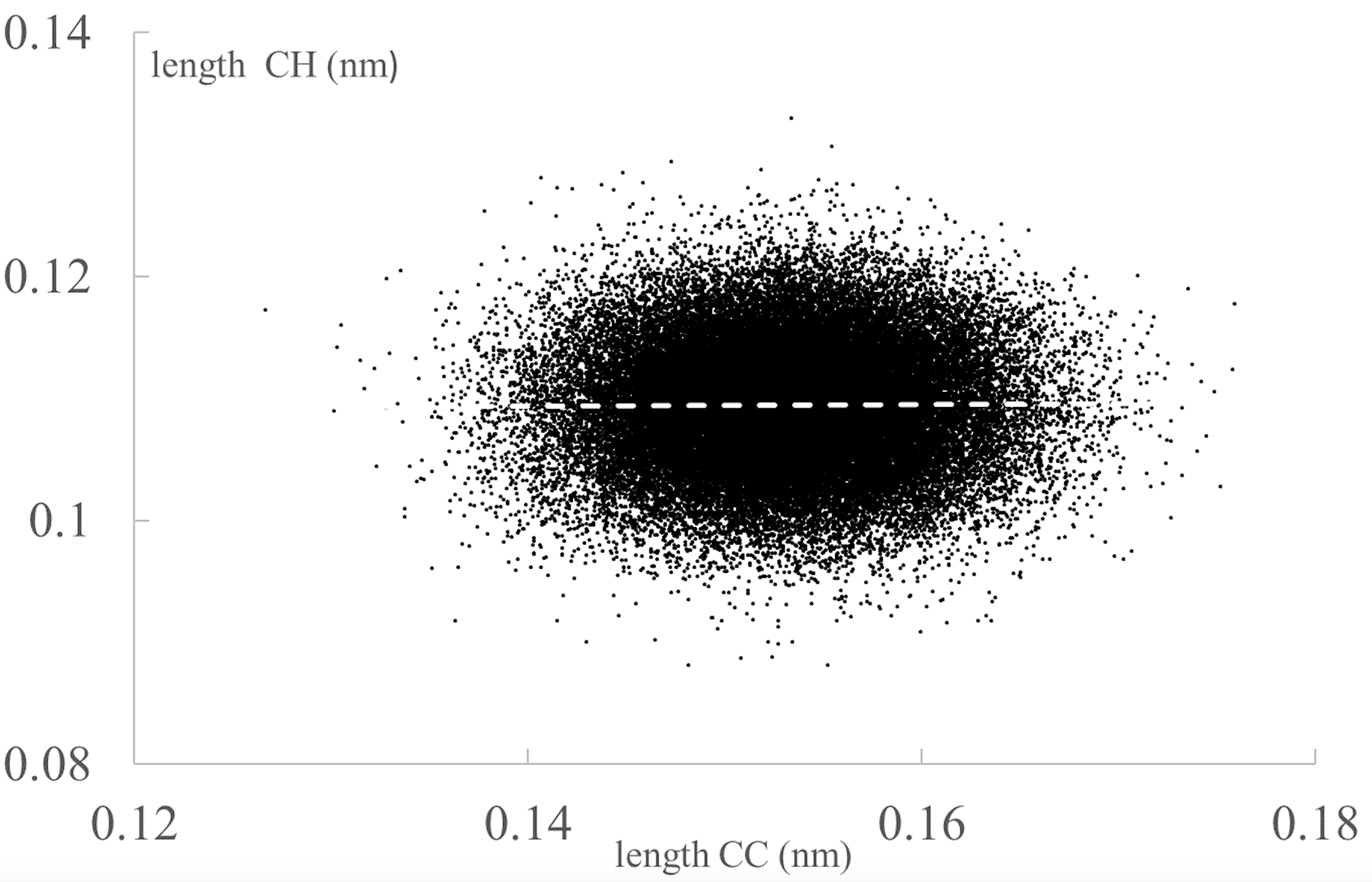
Figure 2: Correlation of length ${C_{3}H_{13}}$ according to the length ${C_{2}C_{3}}$. Dashed regression line.

The distribution of points is apparently random within the cloud. The elliptical shape is due to the difference in equilibrium lengths of CC bonds (${\bf eq}_{{CC}}={0.1529}\>\mathit{nm}$) and CH bonds (${\bf eq}_{{CH}}={0.109}\>\mathit{nm}$). The magnitude of the distribution is directly related to the temperature and therefore to the amplitude of variation of the bond lengths relative to their equilibrium value. The treatment of this distribution by a linear regression of least squares method gives a zero slope, with a precision of $10^{-5}$. The same analysis has been applied to the 3 other CH bonds coupled to ${C_{2}C_{3}}$ (${C_{2}H_{10}}$, ${C_{2}H_{11}}$, ${C_{3}H_{12}}$) with an identical result. More generally, there is an absence of correlation between ${C_{2}C_{3}}$ and any CH bond of the molecule. The lack of correlation with the coupled CH bonds has also been checked for the other CC bonds (${C_{0}C_{1}}$, ${C_{1}C_{2}}$, ${C_{3}C_{4}}$ and ${C_{4}C_{5}}$). Thus, the result is always the same : there is no correlation in time between the lengths of the CC and CH bonds. This results have been confirmed on longer molecules. Therefore, the correlation factor ${\bf{A}}$ in equation (10) is equal to 0 which implies that the CC and GG bond potentials are identical:

$$k_{GG}=k_{CC}={{268}\>kcal/mol/{\text{\AA}}^{2}}$$ (14)

3.2 Correlation Analysis of CCC Valence Angles

The same method is applied to the correlation analysis of the angle of valence ${C_{2}C_{3}C_{4}}$ of the molecule ${C_{\mathit{6}}H_{\mathit{12}}}$ with the CCH and HCH angles. It can be seen that the values of the angles that are uncoupled to ${C_{2}C_{3}C_{4}}$ have a zero correlation with this one. On the other hand, angle ${H_{12}C_{3}H_{13}}$ (the HCH angle attached to carbon $C_{3}$) has a non-zero correlation with the angle ${C_{2}C_{3}C_{4}}$. The corresponding cloud of points is shown on the left side of Fig. 3.

The regression slope is $-0.21\pm 0.003$. The negative value of the slope means that, on average, the HCH angle has a value less than its equilibrium value ${\bf eq}_{{HCH}}$ when the CCC angle has a value greater than its equilibrium value ${\bf eq}_{{CCC}}$. The value of the slope of regression equals ${\bf{C}}.{\bf eq}_{{HCH}}/{\bf eq}_{{CCC}}$. Like the ratio of equilibrium angle values ${\bf eq}_{{HCH}}/{\bf eq}_{{CCC}}$ is $108.4/112.7=0.962$, the correlation coefficient ${\bf{C}}$ is $-0.21/0.962=-0.218$. As a result, the correlation is only partial, which implies that the energy of the the angle ${H_{12}C_{3}H_{13}}$ only partly participates in the energy of the angle ${C_{2}C_{3}C_{4}}$. Of all the CCH angles, only the four angles ${C_{2}C_{3}H_{13}}$, ${C_{2}C_{3}H_{14}}$, ${C_{3}C_{4}H_{13}}$ and ${H_{14}C_{3}C_{4}}$ have a non-zero correlation with the valence angle ${C_{2}C_{3}C_{4}}$ (the case of ${C_{2}C_{3}H_{13}}$ is shown in the right side of Fig. 3). We can see that the regression slope is the same for all four CCH angles and is $-0.2\pm 0.003$. The regression slope is equal to ${\bf{B}}.{\bf eq}_{{CCH}}/{\bf eq}_{{CCC}}$. Like the ratio ${\bf eq}_{{CCH}}/{\bf eq}_{{CCC}}$ is $110.5/112.7=0.98$, the correlation factor ${\bf{B}}$ is $-0.2/0.98=-0.204$. Therefore, this correlation is also partial. The equation (11) is then written:

$$k_{GGG}=58.35+4(-0.204)^{2}\times(108.4/112.7)^{2}\times 37.5+(-0.218)^{2}\times(110.5/112.7)^{2}\times 33$$ (15)

thus:

$$k_{GGG}={{65.63}\>kcal/mol/{\text{\AA}}^{2}}$$ (16)

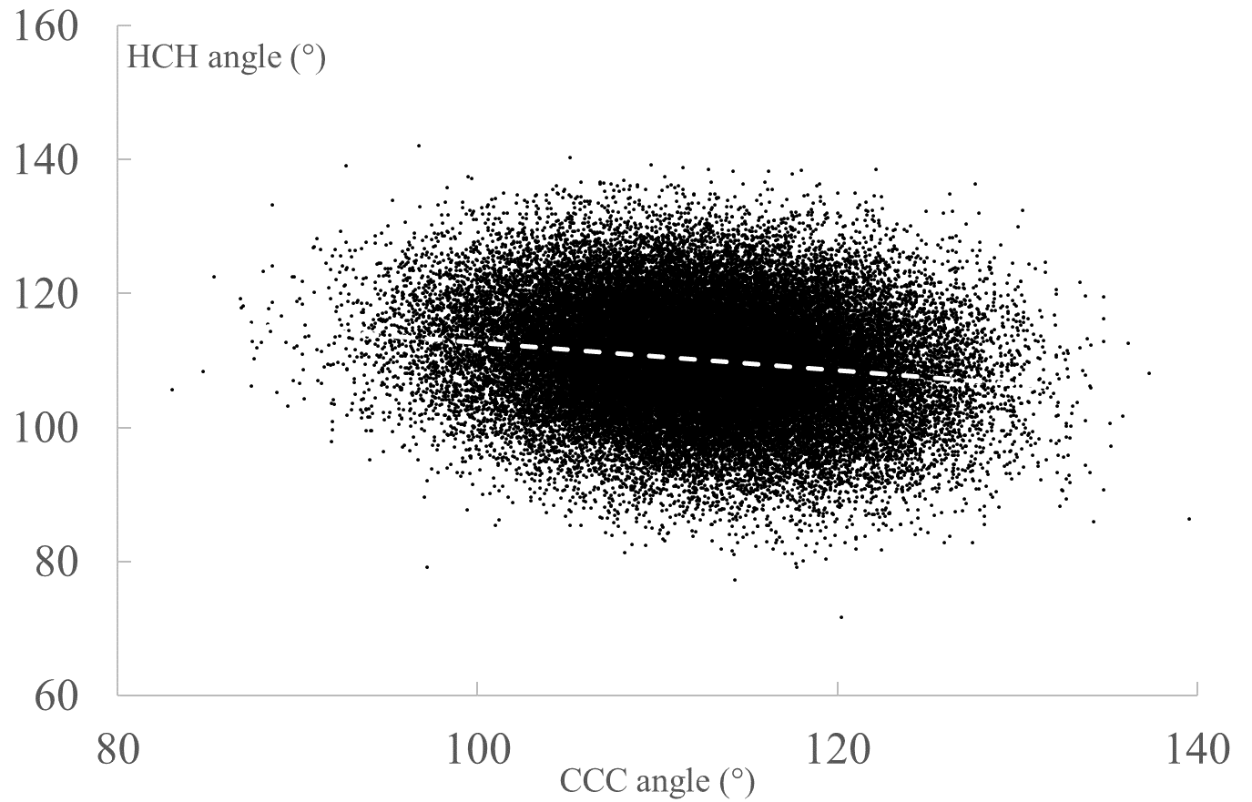
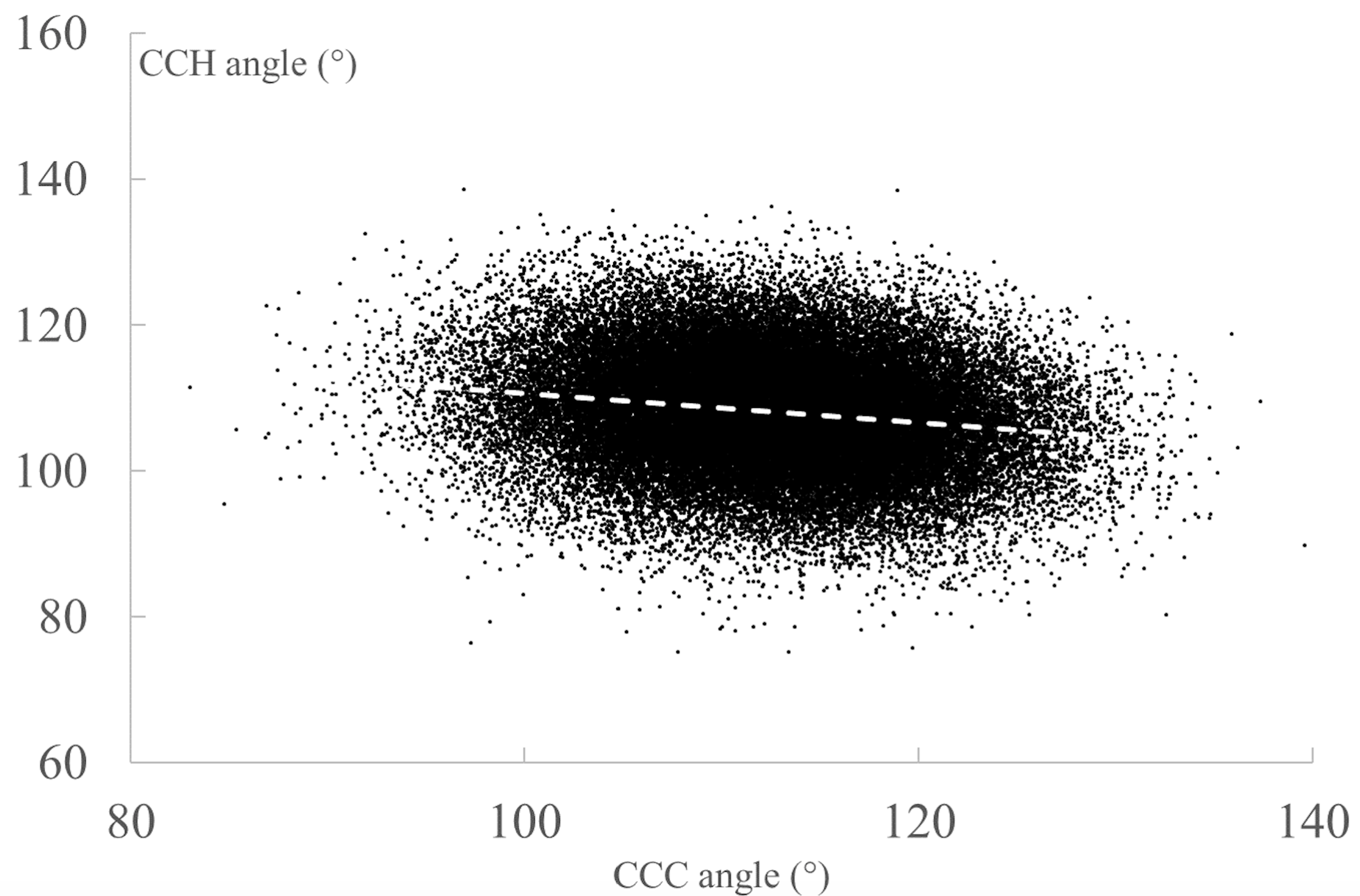
Figure 3: Left Image: correlation of valence angle ${H_{12}C_{3}H_{13}}$ with the angle ${C_{2}C_{3}C_{4}}$. Dashed regression line. Right Image: correlation of valence angle ${H_{2}C_{3}H_{13}}$ with the angle ${C_{2}C_{3}C_{4}}$.

3.3 Correlation Analysis of CCCC Dihedral Angles

We now apply the correlation analysis between a dihedral angle CCCC and the dihedral angles comprising at least one hydrogen, HCCH and CCCH. As a reference, we retain the angle ${C_{1}C_{2}C_{3}C_{4}}$ that is coupled to the following angles: ${H_{10}C_{2}C_{3}C_{4}}$, ${H_{11}C_{2}C_{3}C_{4}}$, ${C_{1}C_{2}C_{3}H_{12}}$, ${C_{1}C_{2}C_{3}H_{13}}$, ${H_{10}C_{2}C_{3}H_{12}}$, ${H_{11}C_{2}C_{3}H_{12}}$, ${H_{10}C_{2}C_{3}H_{13}}$ et ${H_{11}C_{2}C_{3}H_{13}}$.

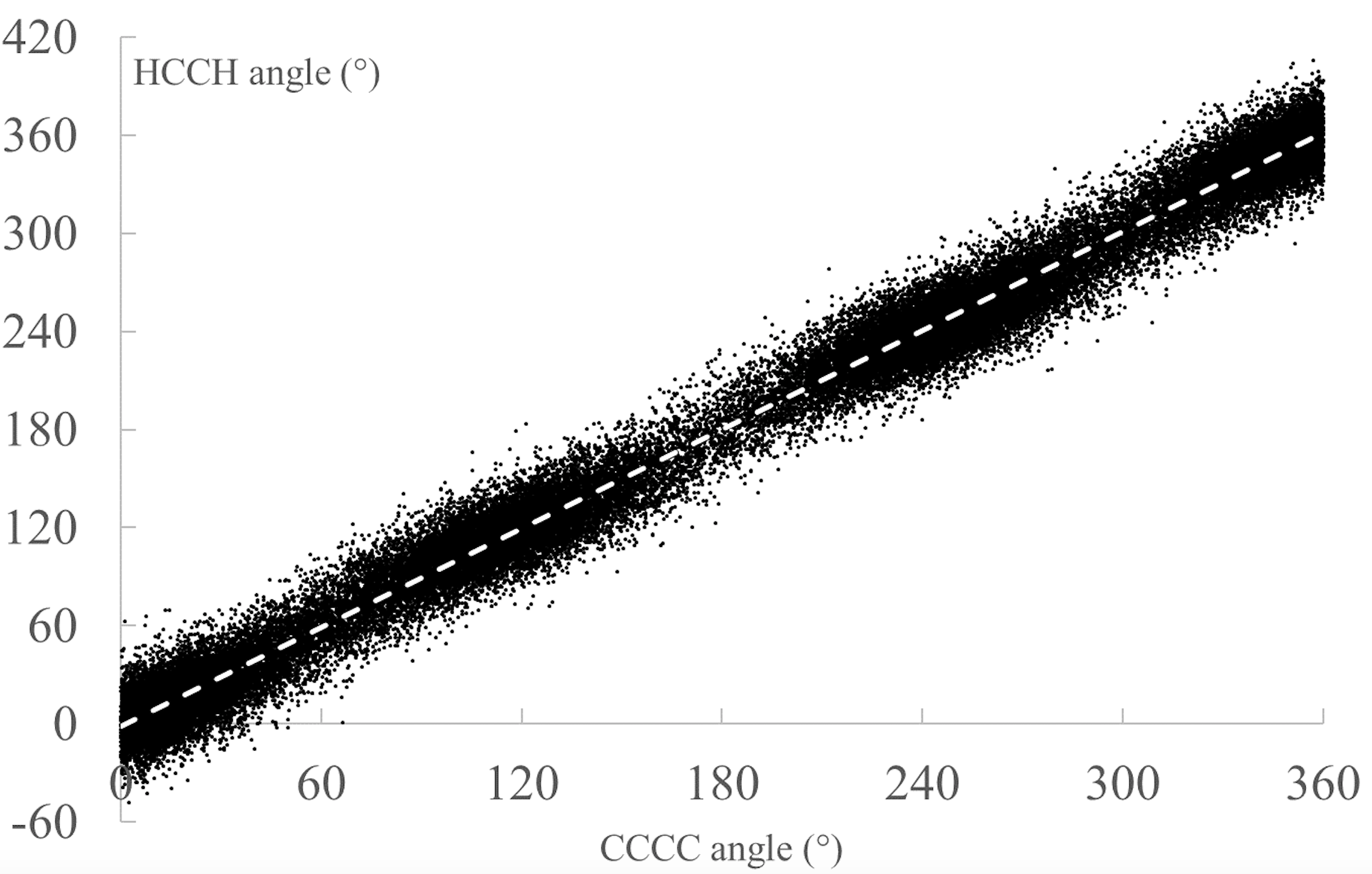
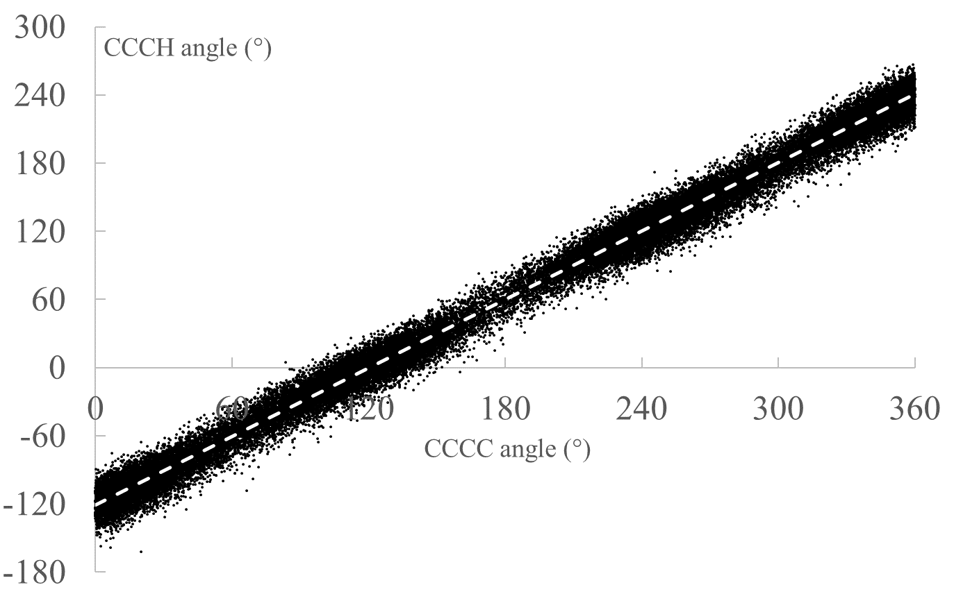
Figure 4: Left Image: correlation of ${H_{11}C_{2}C_{3}C_{4}}$ with the dihedral angle ${C_{1}C_{2}C_{3}C_{4}}$ (dashed regression line). Right Image: correlation of ${H_{11}C_{2}C_{3}H_{13}}$ with the dihedral angle ${C_{1}C_{2}C_{3}C_{4}}$.

The first striking fact is that all the analyses give a slope regression line equal to $1\pm 0.007$. So there is an equal relationship between the angular variations of the angle ${C_{1}C_{2}C_{3}C_{4}}$ and the variations of the coupled angles CCCH and HCCH. The distribution of the angular values on either side of the regression line is related to the kinetic energy of vibration exchanged with the other dihedral angles.

The second striking fact is that the angles considered only differ by their angular phase-shift, given by their ordinate at origin.

The angular shifts, resulting from linear regression, have a periodicity of ${120}^{o}$ (Table 1). The angles are perfectly correlated: when the CCCC angle varies, it directly drives the eight dihedral angles coupled to it. One thus has: ${\bf{D}}={\bf{E}}=1$.

angular phase-shift	dihedral angles
$-{120}^{o}$	$H_{11}C_{2}C_{3}C_{4}$      $C_{1}C_{2}C_{3}H_{14}$      $H_{12}C_{2}C_{3}H_{13}$
${0}^{o}$	$H_{11}C_{2}C_{3}H_{13}$    $H_{12}C_{2}C_{3}H_{14}$
${120}^{o}$	$H_{12}C_{2}C_{3}C_{4}$      $C_{1}C_{2}C_{3}H_{13}$      $H_{11}C_{2}C_{3}H_{14}$

Table 1: Phase-shifts of the dihedral angles coupled to $C_{1}C_{2}C_{3}C_{4}$

.

The perfect correlation between a CCCC dihedral angle and the dihedral angles coupled to it is also checked for the two other CCCC dihedral angles of the ${C_{\mathit{6}}H_{\mathit{12}}}$ molecule. One also observes the same perfect correlation in the case of longer molecules, which makes the result quite general. Because of this correlation and of the modulo ${120}^{o}$, we got:

$${\cal U}_{GGGG}(\phi)={\cal U}_{CCCC}(\phi)+4.{\cal U}_{CCCH}(\phi)+4.{\cal U}_{HCCH}(\phi)$$ (17)

Hence finally:

$${P_{{GGGG}_{1}}}={P_{{CCCC}_{1}}}=1.74~{}kcal/mol$$

$${P_{{GGGG}_{2}}}={P_{{CCCC}_{2}}}=-0.157~{}kcal/mol$$ (18)

$${P_{{GGGG}_{3}}}={P_{{CCCC}_{3}}}+4.{P_{{CCCH}_{3}}}+4.{P_{{HCCH}_{3}}}=3.015~{}kcal/mol$$

Conclusion.

The three components of the intra-molecular UA potential (GG bonds, GGG valence angle, and GGGG dihedral angle) were determined (Eq. (14), (16), (18) by a correlation analysis.

A CC bond oscillator is totally decorrelated in time of the CH oscillators. This implies that the vibration of the GG oscillator is the same as that of the CC oscillator. Thus, the potential energies of the CC and of the GG oscillators are identical. There is no contribution of the potential energy of the CH oscillators to the potential energy of the GG bond.

On the contrary, the dihedral angle oscillators CCCC and CCCH as well as HCCH are totally correlated. Changing the value of a CCCC angle results in the same angular variation of the CCCH and HCCH that are coupled with it. Therefore, the potential energy of a dihedral angle GGGG is the sum of the potential energies of the corresponding CCCC angle with the potential energies of the dihedral angles CCCH and HCCH coupled to it (sharing with it the two central carbons).

Valence angles present an intermediate case. Because of the weak coupling (${\bf{B}}\approx{\bf{C}}\approx-0.2$), the GGG and CCC potentials are different, but only a small percentage of the contribution to GGG’s potential energy is made by the CCH and HCH angles. It should be noted that this is not a driving effect since, in fact, the CCC angles and the CCH and HCH angles vary in the opposite direction.

It should also be noted at this point that if the masses driven by the grains during the UA simulations were depending on the previous correlations, these masses should be different for bonds and for valence angles. That would certainly be a contradiction in terms on a physical level. This issue will be considered in more detail in the next section.

4 Validation of the UA Potential

The main objective of UA simulations is to obtain kinematics in UA as close as possible to those in AA. This proximity of kinematics is of course only sought for the same chain length, at the same temperature, and starting from the same initial condition. Thus, we will compare the kinematics of an AA molecule and that of the corresponding UA molecule, at the same temperature, the UA grains being initially at the same positions as the carbon atoms of the AA molecule.

One immediately notes that, because of the number of atoms involved, the global kinematics of the molecules at both scales cannot be strictly identical, except for very short periods of time (consequence of Poincaré’s three-body theory [11]; we are in a framework of deterministic chaos). In fact, the divergence of the kinematics results from a minute difference, either in the initial conditions, or in the parameters of the UA potentials. A very small difference of one of these values (> $10^{-10}$) causes a divergence in a delay of the order of ${10}\>\mathit{ps}$.

Only average values from the kinematics can therefore be compared. Two kinematics, one in AA and the other in UA, will be consistent if they explore the same phase space. From this point of view, several comparison criteria are possible:

1. Comparison of the average periods of vibration of the corresponding harmonic oscillators (e.g. CC bond and corresponding GG bond).

2. Comparison of mean energies obtained by a Boltzmann-inverse approach using probabilities of presence as a function of length (bond) or angle (valence or dihedral), at both scales.

3. Comparison of the mean end-to-end distances (distances between the two carbons or grains at the extremities) of an AA molecule and of the corresponding UA molecule.

It is important to note that these three criteria are independent of each other and that the first two are at the local scale (level of each oscillator), while the third is at the global scale (complete molecule).

4.1 Comparison of Mean Vibration Periods

The period of vibration $T$ of a harmonic isolated oscillator composed of two mass objects $m_{1}$ and $m_{2}$ is defined by:

$$T=2\pi\sqrt{0.5\times m_{r}/k}$$ (19)

where $m_{r}$ is the reduced mass $m_{r}=1/(1/m_{1}+1/m_{2})$ and $k$ is the stiffness constant of the oscillator. In the case of an oscillator composed of two carbons, we have $m_{r}={{6}\>{g/mol}}$ and $k={{112.1312}\>kg/mol/nm^{2}}$ $({{268}\>kcal/mol/{\text{\AA}}^{2}})$ [4]. The period of this isolated CC oscillator is thus $T={32.45}\>\mathit{fs}$, and this whatever the temperature.

Using a Fourier transform (FFT), the period of vibration of the isolated CC oscillator can be extracted and measured from simulation data. Thus, from a simulation (at ${{300}\>K}$) generating $2^{16}$ measurements (time-steps), the measured vibration period, corresponding to the single vibration peak, is indeed the expected one of ${32.45}\>\mathit{fs}$ (Fig. 5).

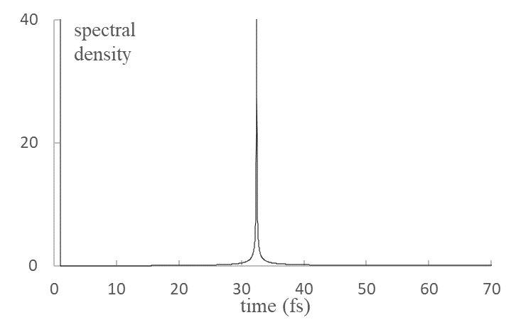
Figure 5: Analysis by FFT of the isolated CC oscillator.

It’s a different situation with a harmonic non-isolated oscillator. In this case, indeed, several peaks appear in the Fourier transform and we can no longer speak of "the" period of vibration of the oscillator. The simplest case of non-isolated oscillator is the CC bond within a ${C_{\mathit{2}}H_{\mathit{4}}}$ molecule. An analysis by FFT of the molecular dynamics of this molecule at ${{20}\>K}$ shows 3 peaks (left image of the Fig. 6).

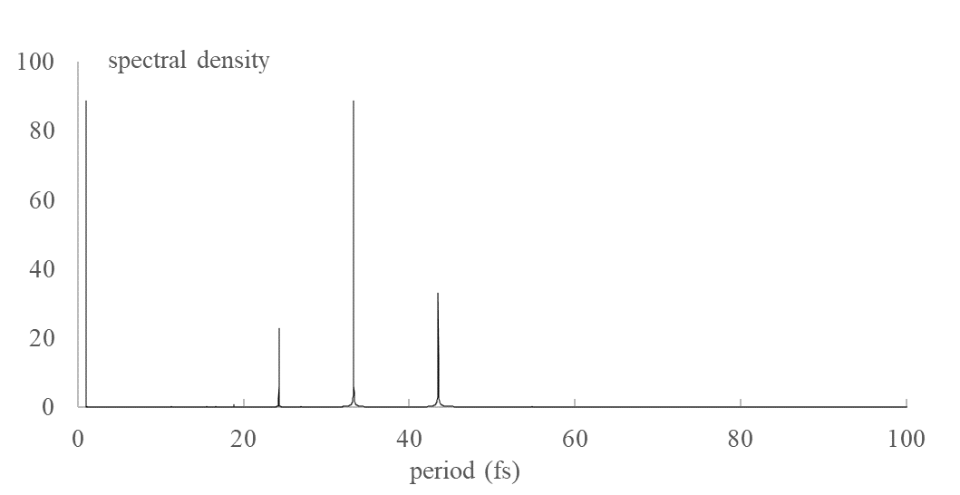
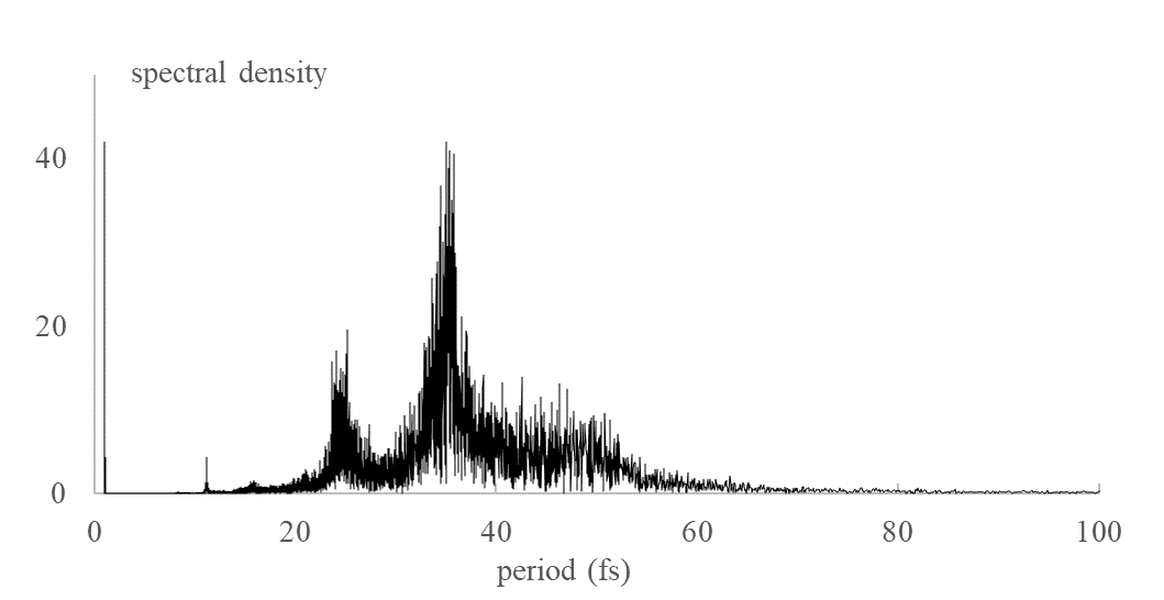
Figure 6: Analysis by FFT of the dynamics of the CC bond in an ${C_{\mathit{2}}H_{\mathit{4}}}$ molecule. Left Image: temperature is ${{20}\>K}$. Right Image: temperature is ${{1000}\>K}$.

The main peak corresponds to a period of ${33.3}\>\mathit{fs}$, i.e. a value significantly different from that of the isolated CC oscillator (${32.45}\>\mathit{fs}$). The number of peaks increases with the temperature (the right image of the Fig. 6 shows the peaks obtained at ${{1000}\>K}$).

The number of peaks also increases with the size of the molecule. Various molecules from $C_{2}H_{4}$ to $C_{100}H_{200}$, various CC bonds in these molecules and various temperatures were considered. The Fig. 7 shows the peaks obtained with the molecule $C_{100}H_{200}$ at both temperatures of ${{100}\>K}$ and ${{1000}\>K}$.

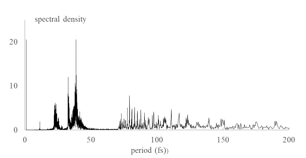
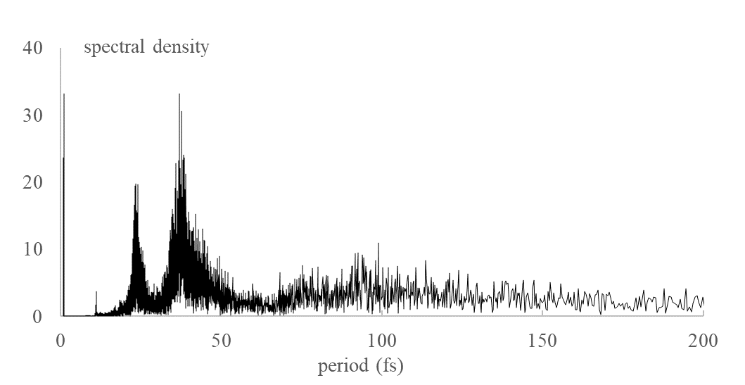
Figure 7: Analysis by FFT of the dynamics of the bond $C_{1}C_{2}$ in a molecule ${C_{\mathit{100}}H_{\mathit{200}}}$. Left Image: temperature is ${{100}\>K}$. Right Image: temperature is ${{1000}\>K}$.

If we cannot speak of "the" period of a non-isolated harmonic oscillator, we are nevertheless going to define its mean period which is that of an isolated harmonic oscillator equivalent, in a sense that we are going to specify now.

The starting point is the Fourier transform of a non-isolated harmonic oscillator whose vibration frequency is considered to be disturbed by interactions with other oscillators. These interactions lead to a degeneration of the vibration peak of the isolated oscillator producing a multiplicity of $N$ peaks. Thus, each peak corresponds to an "interaction mode" of the oscillator with the other oscillators and its spectral density $D_{i}$ reflects the probability $P_{i}$ that the oscillator is in the "mode" corresponding to the peak. The probabilities are defined by:

$$P_{i}=D_{i}/\sum_{1}^{N}{D_{j}}$$ (20)

Each natural frequency $T_{i}$ corresponds to a sinusoidal signal in time which can be considered as produced by a fictitious isolated harmonic oscillator. It has the same stiffness $k$ as that of the non-isolated oscillator, and whose mass $m_{i}$, called fictitious reduced mass, is obtained from the equation (19) by:

$$m_{i}=kT_{i}^{2}/2\pi^{2}$$ (21)

The dynamic reduced mass $mr_{D}$ of a non-isolated oscillator is then defined as the sum of the fictitious reduced masses of the various fictitious oscillators, weighted by their probability $P_{i}$:

$$mr_{D}=\sum_{1}^{N}{P_{i}m_{i}}=(k/2\pi^{2})\sum_{1}^{N}{P_{i}T_{i}^{2}}$$ (22)

The dynamic mass $m_{D}$ is twice the dynamic reduced mass:

$$m_{D}=2\times mr_{D}$$ (23)

The average period $T_{D}$ of a non-isolated harmonic oscillator is then defined as that of the isolated harmonic oscillator of the same stiffness and whose mass is the dynamic reduced mass of the non-isolated oscillator:

$$T_{D}=2\pi\sqrt{0.5\times mr_{D}/k}$$ (24)

Results.

All the FFT analyses performed give for the AA bonds dynamic masses having the same value of $14\pm 0.2~{}g/mol$ with an average period $T={35.05}\>\mathit{fs}$, whatever the temperature.

The determination of dynamic masses can also be carried out at the UA level. For example, we find that the dynamic mass of a GG bond is in all cases (different molecule lengths and different temperatures) ${{14}\>{g/mol}}$. Thus, the dynamic masses of the bonds are the same in AA and UA. With equal stiffnesses in UA and AA, the average periods of AA and GG bonds are the same. This result means that, with equal stiffnesses in AA and UA, the first (local) criterion for comparison between AA and UA is verified for bonds.

A similar analysis of the kinematics of the CCC valence angles in AA also leads to the conclusion that the average dynamic mass of the valence angles is ${{14}\>{g/mol}}$. With approximately the same stiffnesses of the CCC and GGG valence angles, the mean periods of the valence angles are very close in AA and UA, so that the first criterion for comparison between AA and UA is also verified for the valence angles.

If, instead of using the dynamic mass of the oscillators, we took the static mass (${{12}\>{g/mol}}$ in AA and ${{14}\>{g/mol}}$ in UA), we could think that, to obtain equal periods, we would simply fix the stiffness $k^{\prime}_{GG}$ of the GG bond as $k^{\prime}_{GG}=(14/12)\times k_{CC}={{312.67}\>kcal/mol/{\text{\AA}}^{2}}$. This would give us a new UA potential, called modified potential. Several simulations were carried out using this modified potential and the average vibration period obtained is ${32.5}\>\mathit{fs}$ which does not correspond to the average period observed during the simulations of aliphatic molecules in AA. The modified potential is thus not the desired potential because it makes the mean periods of the CC and UA bonds different, leading to divergent kinematics.

In conclusion, the fact that in AA and UA, on the one hand, the stiffness of the bonds are equal and, on the other hand, that the stiffness of the valence angles are equal has the effect of making the average periods of the corresponding oscillators equal. This is the first (local) criterion for comparison between AA and UA.

4.2 Comparison of Energies Obtained by Boltzmann-Inverse

Oscillators, whether AA or UA, are now analyzed by a Boltzmann-inverse method. In this approach, the energy of an oscillator is obtained from the densities of probability of presence in a given state. The formula defining the energy $U$ is :

$$U=k_{B}\times T\times ln(P_{0}/P_{i})$$ (25)

where $k_{B}$ is the Boltzmann constant, $T$ is the temperature of simulation, $P_{0}$ is the maximum probability and $P_{i}$ is the probability of state $i$. The treatment of bonds and valence and dihedral angles is performed from the same simulation in molecular dynamics. The range of variation of the values has been segmented into 200 evenly distributed classes and the probabilities of presence in each class have been obtained from $10^{6}$ time-steps.

The energies of the CC and GG bonds, of the CCC and GGG valence angles, and of the CCCC and GGGG dihedral angles, were compared for the two molecules ${C_{\mathit{16}}H_{\mathit{32}}}$ and $G_{16}$, at a temperature of ${{300}\>K}$. The same analysis was also performed, with the modified potential defined in the section 4.1. The results obtained are shown in Fig. 8.

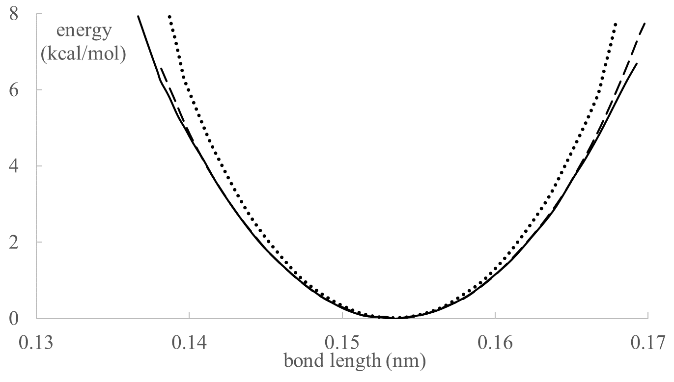
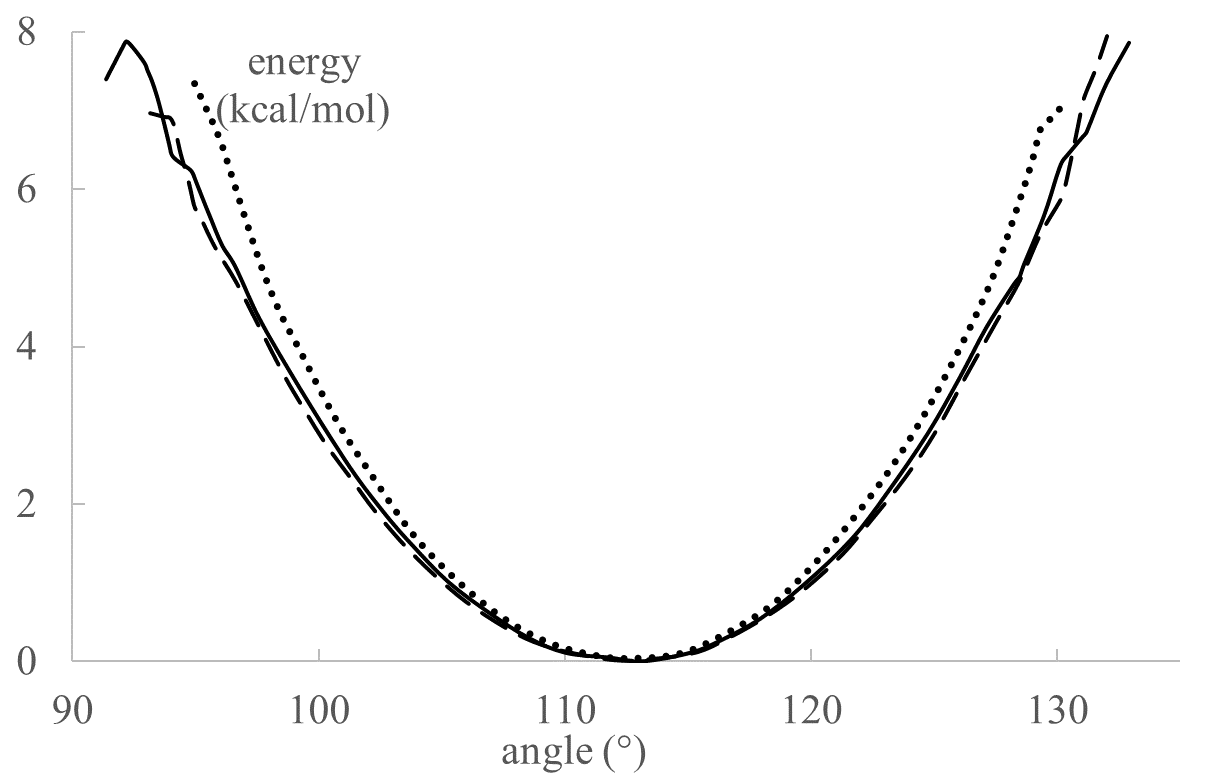
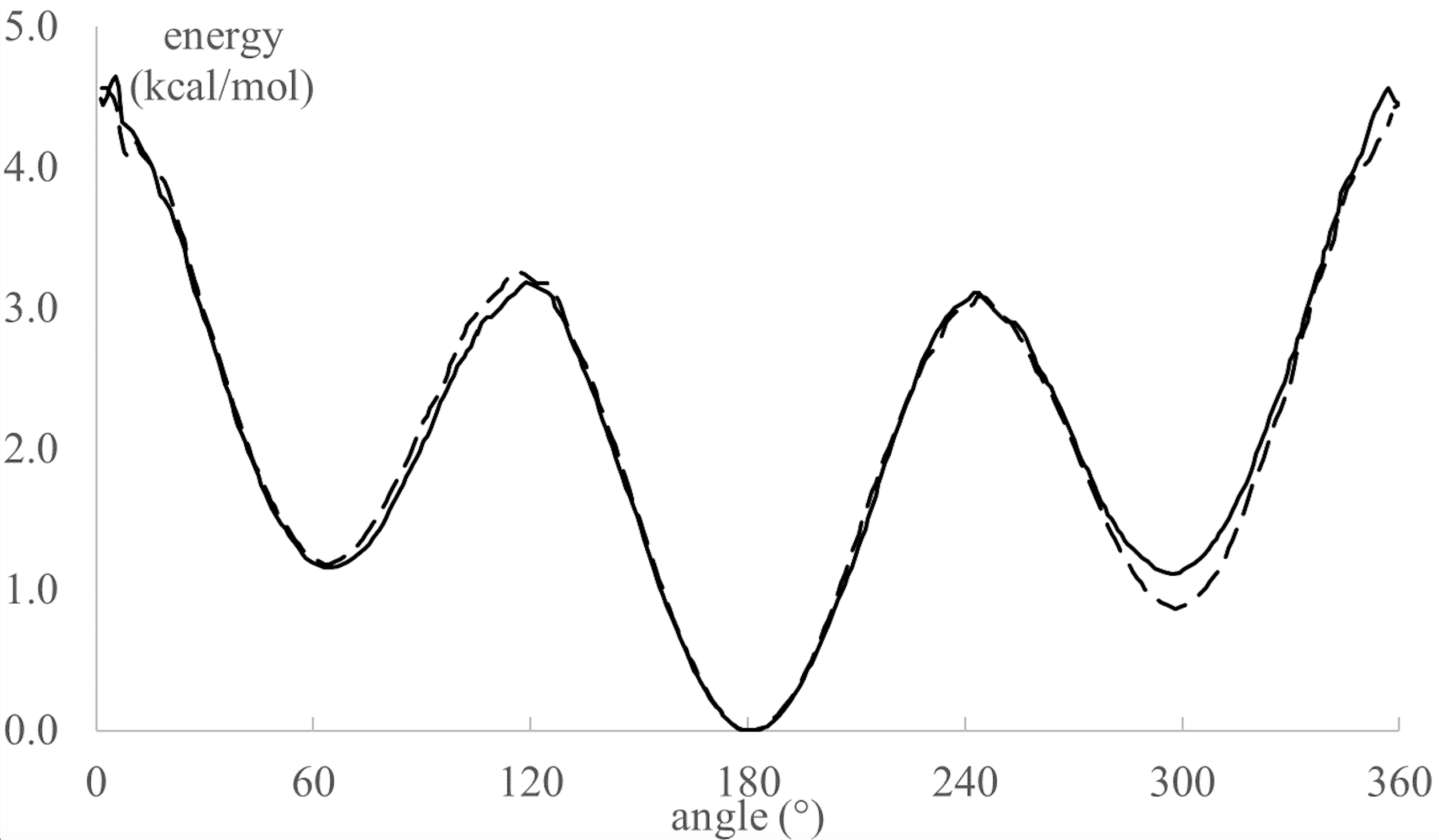
Figure 8: Boltzmann-inverse analysis of an ${C_{\mathit{16}}H_{\mathit{32}}}$ (solid line), a $G_{16}$ molecule (dashed line) and the same $G_{16}$ molecule with the modified potential (dotted line). Left Image: bonds. Right Image: valence angles. Middle Image: dihedral angles.

One notices that the energies determined by Boltzmann-inverse for the molecules ${C_{\mathit{16}}H_{\mathit{32}}}$ and $G_{16}$ coincide very precisely. This result has been verified on longer molecules and at different temperatures. As regards the modified potential, the results are unambiguous: it gives systematically higher energies which confirms that this potential is not the one we are looking for and that the dynamic mass is indeed ${{14}\>{g/mol}}$.

This second analysis at the local scale shows that the energies obtained by Boltzmann-inverse from AA and UA are well consistent.

4.3 Comparison of End-to-End Distances

Molecular conformational changes on a global scale depend mainly on dihedral angles, moving from trans conformations to gauche (or gauche’) conformations or vice-versa. The gauche conformations reduce the distance between the ends of the molecule, called the end-to-end distance (EtE). One has analyzed the EtE distances of ${C_{\mathit{16}}H_{\mathit{32}}}$ and $G_{16}$ molecules. These distances fluctuate widely over the time due to the conformational changes. One lets temperatures vary from ${{100}\>K}$ to ${{2000}\>K}$ in steps of ${{50}\>K}$. The results are shown on Fig. 9.

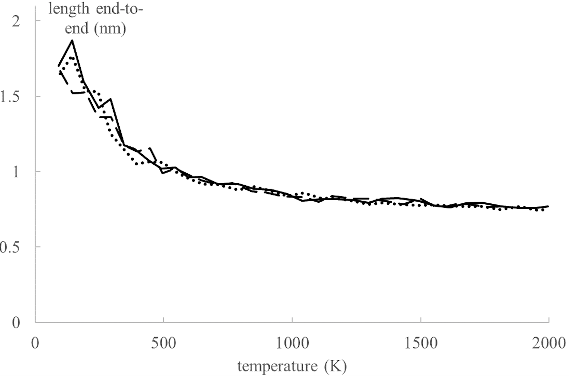
Figure 9: Distances ${\it EtE}$ of ${C_{\mathit{16}}H_{\mathit{32}}}$ (solid line), $G_{16}$ (dashed line) and $G_{16}$ with the modified potential (dotted line).

One can see that the average EtE distances decrease when the temperature increases, both in AA and UA, and that the results in UA are very close to the results in AA.

Very similar results are obtained using the modified potential introduced in 4.1. which suggests the EtE analysis is less sensitive to UA force field parameters than the local analysis.

Let us note that an EtE analysis of a $C_{16}$ molecule was described in [2] at a temperature of ${{373}\>K}$. The conclusion of this analysis, which differs from the one presented here, is that the EtE distances in AA are greater than in UA.

5 Conclusion

A method was presented for deriving an UA potential from an AA potential based on an analysis of the correlations that may exist between coupled oscillators (e.g. CC and CH bonds). The analyzed data are generated in molecular dynamics by simulations with durations in the nano-second range. The method was applied to isolated alkanes, simulated from the OPLS-AA potential, and the intra-molecular components of the corresponding UA potential were determined. The resulting bond stiffness constants and dihedral angle constants are the same as those in the article [6] defining OPLS-AA. We provide a justification, in terms of correlations, for the values of these constants. However, the stiffness of the obtained UA valence angle potential differs from that of [6] (${{65.63}\>kcal/mol/{\text{\AA}}^{2}}$ instead of ${{58.35}\>kcal/mol/{\text{\AA}}^{2}}$). Moreover, the UA potentials obtained do not depend on the size of the molecules, contrary to those of [6].

The method was validated by comparing the results of AA and UA simulations of similar molecules, at the same temperature, according to different criteria: mean end-to-end lengths of the molecules ; mean periods of vibration of the oscillators ; energies obtained by Boltzmann-inverse analysis, based on the state probabilities of presence. The comparisons made show the close proximity of the global kinematics of the AA and UA molecules.

The carbon atoms of all AA oscillators have the same dynamic mass of ${{14}\>{g/mol}}$, which means that the hydrogens are driven by the carbons to which they are bound. Note that this does not necessarily imply that hydrocarboned oscillators are correlated to the carboned oscillators to which they are coupled. Hence, there is no temporal correlation in the case of bonds, whereas the correlation is total in the case of dihedral angles, and only partial in the case of valence angles.

The correlation method seems to be easily applicable to molecules other than alkanes.

References

- [1] M.P. Allen and D.J. Tildesley. Computer Simulation of Liquids. Oxford, 1987.
- [2] R. Baron, A.H. de Vries, P.H. Hünenberger, and W.F. van Gusteren. Comparison of Atomic-Level and Coarse-Grained Models for Liquid Hydrocarbons from Molecular Dynamics Configurational Entropy Estimates. J. Phys. Chem., pages 8464–8473, 2006.
- [3] F. Boussinot, B. Monasse, and J-F. Susini. Reactive Programming of Simulations in Physics. International Journal of Modern Physics C, 26(12), 2015. http://dx.doi.org/10.1142/S0129183115501326.
- [4] W. Damm, A. Frontera, J. Rirado-Rives, and W. L. Jorgensen. OPLS All-Atom Force Field for Carbohydrates. Journal of Computational Chemistry, 18(16):1955–1970, 1997.
- [5] W. L. Jorgensen. Optimized Intermolecular Potential Functions of Liquid Alcohols. J. Phys. Chem., 90:1276–1284, 1986.
- [6] W. L. Jorgensen, J.D. Madura, and C.J. Swenson. Optimized Intermolecular Potential Functions of Liquid Hydrocarbons. J. Am. Chem. Soc., 106:6638–6646, 1984.
- [7] W. L. Jorgensen and D.L. Severance. Aromatic-aromatic Interactions: Free Energy Profiles for the Enzene Dimer in Water, Chloroform and Liquid Benzene. J. Am. Chem. Soc., 112:4768–4774, 1990.
- [8] W. L. Jorgensen and C.J. Swenson. Optimized Intermolecular Potential Functions for Amides and Peptides. Hydration of Amides. J. Am. Chem. Soc., 107:1489–1496, 1985.
- [9] W. L. Jorgensen and J. Tirado-Rives. The OPLS Force Field for Proteins. Energy Minimizations for Crystals of Cyclic Peptides and Crambin. J. Am. Chem. Soc., 110:1657–1666, 1988.
- [10] G. Natta and P. Corradini. General Considerations on the Structure of Crystalline Polyhydrocarbons. Nuovo cimento suppl., 15(Serie X):9–39, 1960.
- [11] H. Poincaré. Sur le problème des trois corps et les équations de la dynamique. Acta Mathematica, (13):1–270, 1890.
- [12] W.H. Reiher. Theoretical Studies of Hydrogen Bonding. PhD Thesis at Harvard University, 1985.
- [13] W.F. van Gusteren and H.J.C. Berendsen. Groningen Molecular Simulation (GROMOS) Library Manual. University of Groningen, the Netherlands, 1987.
- [14] S.J. Weiner, P.A. Kollman, D.A. Case, U.C. Singh, C. Ghio, G. Alagona, S. Profeta, and P.J. Weiner. A New Force Field for Molecular Mechanical Simulation of Uncleic Acids and Proteins. J. Am. Chem. Soc., 106(3):765–784, 1984.
- [15] B. Wunderlich. Macromolecular Physics. Academic Press, 1973.