Dopant levels in large nanocrystals using stochastic optimally tuned range-separated hybrid density functional theory

Abstract

We apply a stochastic version of an optimally tuned range-separated hybrid (OT-RSH) functional to provide insight on the electronic properties of P- and B- doped Si nanocrystals of experimentally relevant sizes. We show that we can use the range-separation parameter for undoped systems to calculate accurate results for dopant activation energies. We apply this strategy for tuning functionals to study doped nanocrystals up to $2.5$ nm in diameter at the hybrid functional level. In this confinement regime, the P- and B- dopants have large activation energies and have strongly localized states that lie deep within the energy gaps. Structural relaxation plays a greater role for B-substituted dopants and contributes to the increase in activation energy when the B dopant is near the nanocrystal surface.

I Introduction

Understanding the properties of dopants in semiconductor nanostructures is a crucial issue for technological applications since it is often the dopants that functionalize a device and control its desired properties.(Ossicini et al., 2006; Norris et al., 2008; Mocatta et al., 2011; Amit et al., 2013; Hori et al., 2016; Li et al., 2018; Lau and Berkelbach, 2019) In particular, doped silicon quantum dots have shown promise in photovoltaic and photonic applications due to their size tunability and processability.(Mavros et al., 2011; Hamid et al., 2013; Somogyi et al., 2017) A key dopant property is its activation energy, which often behaves differently in the nanoscale. For example, when P- (phosphorus) and B- (boron) dopants are introduced to bulk Si, they create shallow impurity states that can act as donors/acceptors of charge carriers. However, in nanocrystals such dopant impurities become deep states due to quantum confinement and dielectric mismatch.

Numerous tools are available to describe dopant properties for extended systems with periodic boundary conditions in a supercell. The state-of-the-art approach is based on a combination of density functional theory (DFT) with many-body perturbation theory (MBPT), typically within the so-called “GW” approximation.(Hybertsen and Louie, 1985, 1986) However, the application of the GW method to large confined systems such as nanocrystals is limited by the steep scaling and the slow convergence with respect to empty states.(Rohlfing and Louie, 2000) Furthermore, the description of optical excitations requires the use of the Bethe-Salpeter equation (BSE), which scales even steeper with system size, limiting its application to small systems.

In recent years, we have developed a set of stochastic orbital techniques (Baer et al., 2013; Neuhauser et al., 2013a, b; Ge et al., 2014; Neuhauser et al., 2014; Gao et al., 2015; Neuhauser et al., 2015; Rabani et al., 2015; Vlĉek et al., 2017, 2018a, 2018b; Chen et al., 2019; Li et al., 2019) which significantly reduce the scaling and computational costs of both the GW and BSE approaches by introducing a controlled statistical error in the calculated observables. This enables the application of both methods to extremely large, experimentally relevant system sizes containing thousands of electrons.(Neuhauser et al., 2014; Rabani et al., 2015; Vlĉek et al., 2017) Some applications, like those involving linear response time-dependent DFT for optical excitations,(Rabani et al., 2015; Vlĉek et al., 2019; Zhang et al., 2020) require the use of a quasiparticle model Hamiltonian, which is not available through the GW method.

Density functional theory has been a major tool for quasiparticle electronic structure calculations, but its local and semi-local approximations poorly predict electronic properties like the fundamental gaps, ionization energies, and electron affinities. This is especially a problem for dopant properties since local approximations can erroneously predict shallow dopant levels when they are in fact deep.(Rurali et al., 2009; Niquet et al., 2010; Lee et al., 2014) Optimally-tuned range-separated hybrid (OT-RSH) functionals offer a solution to this problem.(Livshits and Baer, 2007; Baer et al., 2010) Specifically, the optimally tuned Baer-Neuhauser-Livshits (BNL) functional(Baer and Neuhauser, 2005; Livshits and Baer, 2007) has been shown to provide an accurate description of the fundamental band gaps for molecules, nanocrystals, and bulk materials.(Stein et al., 2010; Refaely-Abramson et al., 2011; Kronik et al., 2012) One of the major strengths of this approach(Salzner and Baer, 2009) is that it can be tuned to the system of interest based on a physical constraint, avoiding the use of empirical fitting parameters that might not reproduce the correct physics. In fact, it has been suggested that hybrid functionals tuned to physical constraints give some of the most reliable electron densities within DFT.(Medvedev et al., 2017)

One of the questions in applying OT-RSH functionals to study dopant properties is this: How do we tune the functional to correctly calculate dopant energies and at the same time maintain accuracy in describing the band structure? Oftentimes, we want to study many different dopant types and locations. Here, the system-specific tunability that is one of OT-RSH’s strengths becomes a liability. Having to repeat the tuning procedure for every dopant structure would quickly become cumbersome and resource intensive.

In this paper, we apply a stochastic formulation of the optimally tuned BNL range-separated hybrid functional (Neuhauser et al., 2015) to study dopant properties in silicon nanocrystals of up to $1600$ electrons. We show that the range-separation parameter for undoped systems also gives accurate results for dopant activation energies. We thus provide a strategy for tuning functionals for doped systems. This strategy may be generalizable for many different dopant types and positions within the nanocrystal. We demonstrate the usefulness of this strategy in conjunction with stochastic techniques to provide insight on dopant properties for nanocrystals of experimentally relevant sizes.

II Theory and computational details

We summarize the main points in the theory of optimally-tuned range-separated hybrid functionals and its stochastic formulation. Consider a zero-temperature ensemble for a system with an average number of electrons equal to $N-x$ , where $N$ is an integer and $x\in\left(0,1\right).$ For this system, the energy curve $E\left(N-x\right)$ should be linear in $x$, so the slope is equal to the negative of the ionization energy, i.e. to $E\left(N\right)-E\left(N-1\right).$ A similar condition holds for $E\left(N+x\right)$ which should be linear in $x$ with a slope equal to the negative of the electron affinity, $E\left(N+1\right)-E\left(N\right)$.

In exact Kohn-Sham (KS) DFT the ionization energy corresponds to the negative of the HOMO energy. Thus, the line $E\left(N-x\right)$ should have a slope equal to the HOMO energy of the $N$ electron system, and the line $E\left(N+x\right)$ should have a slope of the HOMO for the $N+1$ system. That is, in KS-DFT the LUMO of the $N$ electron system is not equal to the HOMO of the $N+1$ system. The difference is due to the derivative discontinuity in the exchange-correlation energy functional as the number of electrons goes from slightly below $N$ to slightly above it.(Perdew et al., 1982; Perdew and Levy, 1997; Mori-Sánchez et al., 2008; Yang et al., 2012; Mori-Sánchez and Cohen, 2014) This behavior of the exact KS functional is not reproduced correctly by local or semi-local KS functionals, such as LDA and the various types of GGAs where the functional exhibits no derivative discontinuity. To compensate for the lack of derivative discontinuity, the energy $E(N\pm x)$ becomes non-linear.(Stein et al., 2012)

One way to account for this lack and for the non-linearity in $E(N\pm x)$ is to use optimally-tuned range-separated hybrid functionals within generalized Kohn-Sham DFT (GKS-DFT).(Livshits and Baer, 2007; Baer et al., 2010; Kronik et al., 2012) Specifically, we employ the range-separated hybrid functional following the proposal by Savin to use full-exchange at long distances.(Savin, 1995; Iikura et al., 2001; Toulouse et al., 2004; Baer and Neuhauser, 2005) The exchange term is divided into long- and short-range components

$$\frac{1}{r}=\frac{\text{erf}\left(\gamma r\right)}{r}+\frac{\text{erfc}\left(\gamma r\right)}{r}$$ (1)

where $\gamma$ is the range-separation parameter that controls the distance upon which the potential is switched from long to short range, $\text{erf}\left(x\right)$ is the error function, and $\text{erfc}\left(x\right)$ is the complimentary error function. The long-range term is calculated explicitly through a Fock-like exchange operator while the short-range term is approximated by a screened local exchange functional.

This hybrid construction is attractive because it maintains the correct long-range asymptotic behavior, decaying as $1/r$, whereas local exchange functionals are known to decay too rapidly. This property allows a full fraction of exact exchange to cancel out the long-range self-interaction error in the Hartree energy part of the DFT functional. A complication is that the range-separation parameter $\gamma$ is in principle a functional of the density that we currently do not know how to construct. This is where the approach of optimally tuning becomes useful.(Livshits and Baer, 2007; Baer et al., 2010)

The tuning of $\gamma$ imposes a physical constraint to the system instead of relying on universal or empirical fittings. The physical constraint ensures that it satisfies the linearity of the ensemble energy $E\left(N\pm x\right)$ with a fractional number of electrons $x$. Since by Janak’s theorem(Janak, 1978) the energy slope is equal to the orbital energy, the constant slope requirement is equivalent to

$$\frac{\partial\varepsilon_{H/L}}{\partial f_{H/L}}=0$$ (2)

where $\varepsilon_{H/L}$ refers to the HOMO or LUMO orbital energy and $f_{H/L}$ is its occupancy. Hence, the approach explicitly constructs a GKS functional such that the IP corresponds to the HOMO and the EA to the LUMO as closely as possible, meaning the functional should be able to accurately describe fundamental band gaps. In many cases, this approach works well and can predict fundamental gaps close to experiment and to MBPT methods for various atomic and molecular systems,(Stein et al., 2010; Refaely-Abramson et al., 2011) as well as Rydberg(Baer et al., 2010) and charge-transfer excitations (within TDDFT).(Stein et al., 2009; Kronik et al., 2012)

Dopant activation energies are calculated similar to fundamental gaps. For electron donors, the activation energy is defined as the energy difference to ionize the dopant and place the electron back into the undoped structure. For acceptors, it is the difference to remove an electron from the undoped structure and place it back into the acceptor level. To summarize,

$$E_{\text{act}}=IP_{d}-EA_{u}$$ [donor]

$$E_{\text{act}}=IP_{u}-EA_{d} \,\,\,\,\,\,\,\text{[acceptor]},$$ (3)

where the subscripts $d$ and $u$ refer to the doped or undoped structures. We can ensure the dopant IPs and EAs are calculated correctly by tuning the functionals to the dopant levels explicitly. However, repeating the tuning procedure becomes costly, especially since one often wants to examine many different dopant types at different dopant locations. One of the key findings of the paper is that we can bypass this tuning step and simply use $\gamma$ for the undoped structure in the spirit of using one constant $\gamma$ for the fundamental gap. In this case, the dopant can be viewed as a perturbation to the electronic structure of the undoped system and does not significantly affect its electronic environment.

A roadblock to using hybrid functionals is that they are much more expensive to use than local multiplicative functionals like the local density approximation (LDA) since they involve the explicit calculation of the orbital-dependent exchange energy. In a “deterministic” (non-stochastic) calculation, the long-range exchange operator is given by the expression:

$$\hat{K}_{x}^{lr}[\psi_{i}(\boldsymbol{r})]=-\sum_{j=1}^{N_{\text{occ}}}\psi_{j}(\boldsymbol{r})\int d\boldsymbol{r}^{\prime}\psi_{j}^{*}(\boldsymbol{r}^{\prime})\psi_{i}(\boldsymbol{r}^{\prime})V_{\text{c}}^{\gamma}(|\boldsymbol{r}-\boldsymbol{r}^{\prime}|)$$ (4)

where $V_{\text{c}}^{\gamma}(|\boldsymbol{r}|)$ is the long-range screened Coulomb potential governed by the range parameter $\gamma$. The computation of this exchange term roughly scales quadratically as $N_{\text{occ}}N_{\text{grid}}$, where $N_{\text{occ}}$ is the number of occupied states and $N_{\text{grid}}$ is the size of the basis set (the number of real-space grid points), both of which increase with system size. In a typical hybrid functional application, this exchange term takes up the overwhelming majority of the total computation time.

Stochastic techniques have been developed to overcome the deterministic scaling limit to make hybrid functional calculations tractable for large systems.(Neuhauser et al., 2015) Using a technique called stochastic resolution of the identity, we can decouple the $\mathbf{r}$ and $\mathbf{r^{\prime}}$ indices in Eq. (4). We introduce a stochastic orbital $\xi(\boldsymbol{r})$ that assigns a random sign to each real-space grid point ($dV$ is the volume per grid point):

$$\xi(\boldsymbol{r})=\langle\boldsymbol{r}|\xi\rangle=\pm\frac{1}{\sqrt{dV}}.$$ (5)

We define

$$\eta(\boldsymbol{r})=\sum_{j=1}^{N_{\text{occ}}}\psi_{i}(\boldsymbol{r})\langle\psi_{i}|\xi\rangle,$$ (6)

which is the stochastic orbital projected on to the occupied space spanned by $\psi_{i\in\text{occ}}(\boldsymbol{r})$. Similarly, we can write the Coulomb potential in a stochastic representation as

$$\zeta(\boldsymbol{r})=\frac{1}{(2\pi)^{3}}\int d\boldsymbol{G}\sqrt{\tilde{V}_{\text{c}}^{\gamma}(\boldsymbol{G})}e^{i\varphi(\boldsymbol{G})}e^{\text{i}\boldsymbol{G}\cdot\boldsymbol{r}},$$

where $\tilde{V}_{\text{c}}^{\gamma}(\boldsymbol{G})$ is the Fourier transform of $V_{\text{c}}^{\gamma}(|\boldsymbol{r}|)$ and $\varphi(\boldsymbol{G})$ is a random phase between $[0,2\pi]$. Now we can rewrite the exchange term in Eq. 4 as an average ($\left\langle\cdots\right\rangle_{\xi,\varphi}$) over the stochastic orbitals:

$$\hat{K}_{x}^{lr}[\psi_{i}(\boldsymbol{r})]=-\left\langle\eta(\boldsymbol{r})\zeta(\boldsymbol{r})\int d\boldsymbol{r}^{\prime}\zeta^{*}(\boldsymbol{r}^{\prime})\eta^{*}(\boldsymbol{r}^{\prime})\psi_{i}(\boldsymbol{r}^{\prime})\right\rangle_{\xi,\varphi}.$$

Defining the product of stochastic orbitals $\chi(\boldsymbol{r})=\zeta(\boldsymbol{r})\eta(\boldsymbol{r})$, we simplify the above expression to

$$\hat{K}_{x}^{lr}[\psi_{i}(\boldsymbol{r})]=-\frac{1}{N_{\text{sto}}}\sum_{\chi=1}^{N_{\text{sto}}}\chi(\boldsymbol{r})\langle\chi|\psi_{i}\rangle.$$ (7)

The scaling for the exchange becomes $N_{\text{sto}}N_{\text{grid}}$, where $N_{\text{sto}}$ is the number of stochastic orbitals. If $N_{\text{sto}}$ goes to infinity, we recover the deterministic result in Eq. (4) exactly. In this sense, $N_{\text{sto}}$ becomes another convergence parameter that we control at the cost of introducing statistical error. Remarkably, we find that $N_{\text{sto}}$ is often independent of system size or can even decrease with system size (see Sec. Results and Ref. Neuhauser et al., 2015 for details), so the scaling for stochastic exchange becomes quasilinear.

We implemented the stochastic BNL functional into a plane wave DFT code to calculate quasiparticle spectra and fundamental gaps for H-passivated Si nanocrystals ranging from 1 to $2.5$ nm in diameter, containing up to $N_{e}\approx 1600$ electrons. We tune the range separation parameter $\gamma$ for each nanocrystal size based on the physical constraint described above. We used a kinetic energy cutoff of $40$ Ry for the density, which converges band gaps to within $0.1$ eV. We treat the divergent $G=0$ term in the exchange energy using the Gygi-Baldereschi method.(Gygi and Baldereschi, 1986) Structural relaxations were performed with Quantum ESPRESSO with the LDA functional.(Giannozzi et al., 2009, 2017) For more computational details, see the Supplementary Material.

III Results

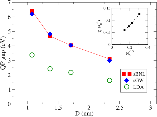
Figure 1: QP gap comparisons for Si NCs ranging from $1$ to $2.5$ nm. The sGW results are from Ref. Neuhauser et al., 2015. Inset: The trend in the optimized $\gamma$s for different NC sizes is nearly linear with respect to $N_{\text{Si}}^{-1/3}$.

Using optimized $\gamma$s obtained from the tuning procedure, in Fig. 1 we compare quasiparticle (QP) gaps for Si NCs of different sizes obtained by different theoretical methods. The agreement between stochastic BNL (sBNL) and stochastic GW (sGW)(Neuhauser et al., 2014; Vlĉek et al., 2017, 2018a, 2018b) is remarkable whereas LDA significantly underestimates the gap. We note that $\gamma$ decreases nearly linearly with system size (see inset in Fig. 1),(Stein et al., 2010; Neuhauser et al., 2015) illustrating the favorable scaling properties of sBNL: Since $\gamma$ becomes smaller as system size increases, the fraction of stochastic exact exchange mixed into the functional also becomes smaller. Therefore, we can use fewer stochastic orbitals to converge the exchange energy to within an acceptable error, which decreases the computation time.

Note that if we extrapolate $\gamma$ to the bulk limit ($N_{\text{Si}}^{-1/3}\rightarrow 0$), we would find $\gamma_{\text{bulk}}$ to be nearly $0$, meaning the exchange is entirely handled by the short-range local functional, which gives incorrect results for the gap. This problem can be addressed by introducing a dielectric coefficient to modulate long-range charge transfer.(Bhandari et al., 2018; Kronik and Kümmel, 2018) Without the dielectric term, we would expect $\gamma$ to saturate at the value of $\gamma=0.02$ (empirically determined) due to exchange-driven orbital localization. This phenomenon has been observed with the BNL functional for 1D chains but has yet to be seen for 3D systems.(Vlĉek et al., 2016) Based on our model, this localization should occur at around $N_{\text{Si}}=8200$, or a system with over $N_{e}=32,800$ electrons.

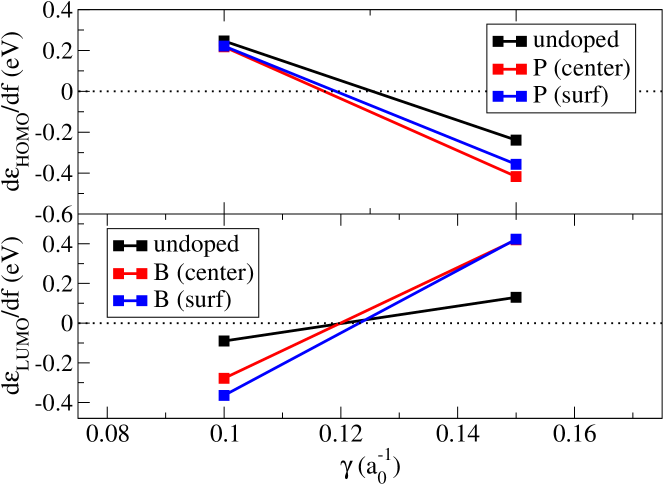
Figure 2: Tuning $\gamma$ for the undoped and doped structures in the $D=1$ nm NC. The optimal $\gamma$ values are given by the intersect with the $y$-axis (dotted line). Upper panel: A partial charge is removed from the HOMO, which is the dopant level for a P donor. Lower panel: A partial charge is added to the LUMO, which is the dopant level for a B acceptor.

system	optimized $\gamma$	energy level	energy level	difference
		at $\gamma$	at $\gamma=0.125$	$\Delta E$
undoped (HOMO)	0.125	N/A	N/A	N/A
undoped (LUMO)	0.120	-1.351	-1.313	0.038
P (center)	0.117	-4.355	-4.387	-0.032
P (surface)	0.119	-4.336	-4.360	-0.024
B (center)	0.120	-4.478	-4.462	0.016
B (surface)	0.123	-4.182	-4.173	0.009

Table 1: Tuning comparisons for $D=1$ nm nanocrystal. $\gamma$s are in units of $a_{0}^{-1}$ and energies in eV. The difference shown is $\Delta E=E(\gamma=0.125)-E(\gamma)$.

Next, we show that $\gamma$s tuned for the undoped structures give reasonable results for doped system properties. We test a P substituted dopant for an electron donor, and a B substituted dopant for an electron acceptor in two dopant locations: one at the center of the nanocrystal, and another near the nanocrystal surface. For the surface dopant, we substitute a four-coordinated Si atom as far from the center as possible. We relax the doped structures in all cases.

In Table 1 we show tuning comparisons for the smallest ($D=1$ nm) nanocrystal. For this system, we repeat the tuning procedure to optimize $\gamma$s for each of the doped structures (Fig. 2). This ensures that the physical constraint for the tuning applies directly to the dopant level itself. When tuning the P-doped structures (donors), we remove a small partial charge ($+0.05e$) from the HOMO; when tuning the B-doped structures (acceptors), we add a partial charge ($-0.05e$) to the LUMO. We plot how much the dopant energies change when using $\gamma$s tuned specifically for the doped structures compared to undoped system $\gamma$. We find the change to be negligible, the largest difference being $32$ meV. This difference is smaller than the change in the undoped structure energy gap ($38$ meV) when using one $\gamma$ for the HOMO and LUMO. We conclude that we can also use one $\gamma$ (the undoped value) to calculate accurate dopant energies. This strategy likely holds for any four-coordinated dopant location, from the center of the crystal to the surface.

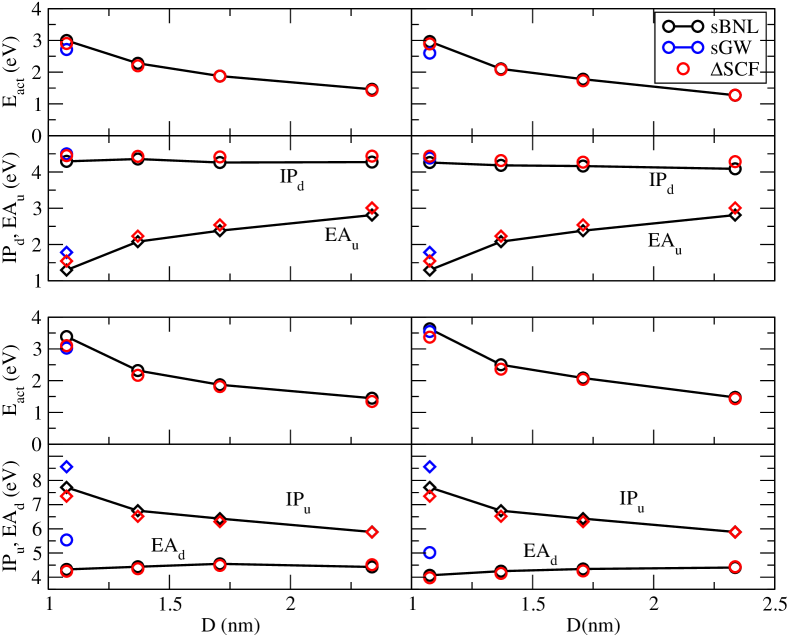
Figure 3: Dopant activation energies for Si NCs with P (upper panels) and B (lower panels) substituted at the center (left panels) and surface (right panels). Component IPs and EAs are also shown. The plotted $\Delta\text{SCF}$ results were performed with the LDA functional.

In Fig. 3 we plot the dopant activation energies, ionization energies, and electron affinities for all nanocrystal sizes. For electron donors like P, we calculate the activation energy as $E_{\text{act}}=IP_{d}-EA_{u}$; for acceptors like B, we calculate the energy as $E_{\text{act}}=IP_{u}-EA_{d}$, where the subscripts $d$ and $u$ refer to the doped or undoped structures. In $\Delta\text{SCF}$, we obtained the IP and EA from total energy differences of charged ($+1e$ or $-1e$) and neutral calculations. In the sBNL and sGW calculations, we obtained the IP and EA from the negative of the corresponding HOMO and LUMO eigenvalue energies (for sBNL) and associated quasiparticle energies (for sGW, see below).

For the sGW calculations, we obtained good agreement with sBNL on the smallest cluster ($D=1$ nm) with the G$\text{W}_{\text{0}}$ energies based on an LDA starting point and with the $\text{G}_{0}$ energies self-consistently iterated.(Vlĉek et al., 2018c) For the larger doped clusters, the LDA results become essentially metallic, so the G$\text{W}_{\text{0}}$ energies are not reliable. Using starting points from other local or semilocal functionals (PBE or even the SCAN metaGGA functional(Sun et al., 2015)) did not improve results. Future studies should examine sGW for dopant energies based on a better starting point, perhaps from the BNL itself.

As a representative data set, Table 2 compares dopant activation energies calculated using different theoretical methods for the $D=1$ nm nanocrystal. As expected, LDA performs poorly, erroneously predicting the dopant level to be nearly shallow. We find that sGW tends to predict deeper energy states than sBNL (seen by the larger IPs and EAs), but the activation energies calculated from the difference of these states agree well with sBNL. Similar energy shifts have been observed in other comparative studies,(Stein et al., 2010; Refaely-Abramson et al., 2011; Neuhauser et al., 2015) where in some cases the BNL functional agrees with IPs from experiment better than GW.(Refaely-Abramson et al., 2011) Interestingly, we find that $\Delta$SCF (over LDA and BNL) gives almost identical results to sBNL. $\Delta$SCF seems to work particularly well when the added (or removed) charge is in a strongly localized state (the $IP_{d}$ in the P-doped system and the $EA_{d}$ in the B-doped system agree remarkably well with sBNL).

	P (center)				B (center)
method	$IP_{d}$	$EA_{u}$	$E_{\text{act}}$	diff.	$IP_{u}$	$EA_{d}$	$E_{\text{act}}$	diff.
sBNL	4.292	1.296	2.996	0.000	7.711	4.323	3.387	0.000
sGW	4.498	1.785	2.713	-0.283	8.565	5.540	3.025	-0.362
LDA	3.173	2.739	0.434	-2.562	6.123	5.591	0.531	-2.856
$\Delta$SCF(BNL)	4.333	1.343	2.990	-0.006	7.795	4.501	3.294	-0.093
$\Delta$SCF(LDA)	4.449	1.546	2.903	-0.093	7.348	4.247	3.101	-0.286

Table 2: Method comparisons for dopant activation energies (eV) in $D=1$ nm crystal. Differences are taken with respect to sBNL.

In the size regime tested ($D=1-2.5$ nm), the defect states from the P- and B- dopants are strongly localized, which can be observed in their charge density plots (Fig. 4). As a result, the defect states lie deep in the gap compared to bulk, reflecting their large ($\geq 1$ eV) activation energies. This also leads to an IP that is roughly independent of NC size for the P-doped system and to an EA that is roughly independent of NC size for the B-doped system, consistent with previous theoretical and experimental studies.(Melnikov and Chelikowsky, 2004; Chan et al., 2008; Cantele et al., 2005; Iori et al., 2007; Fujii et al., 2016)

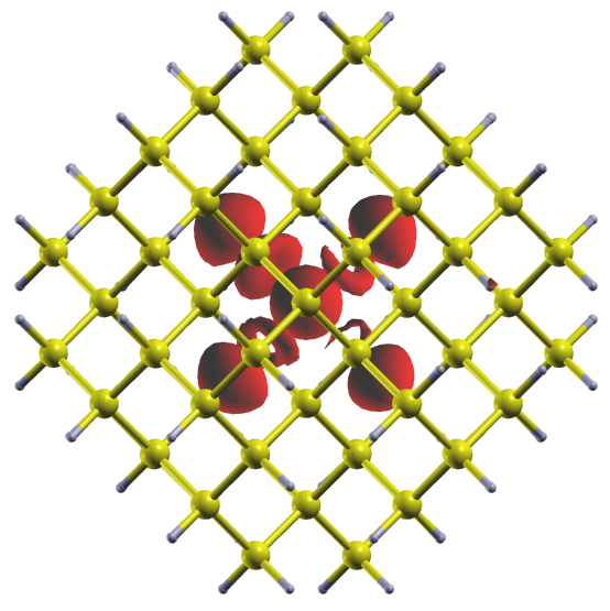
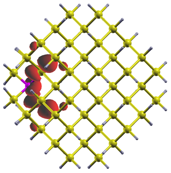
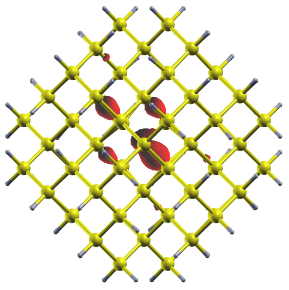
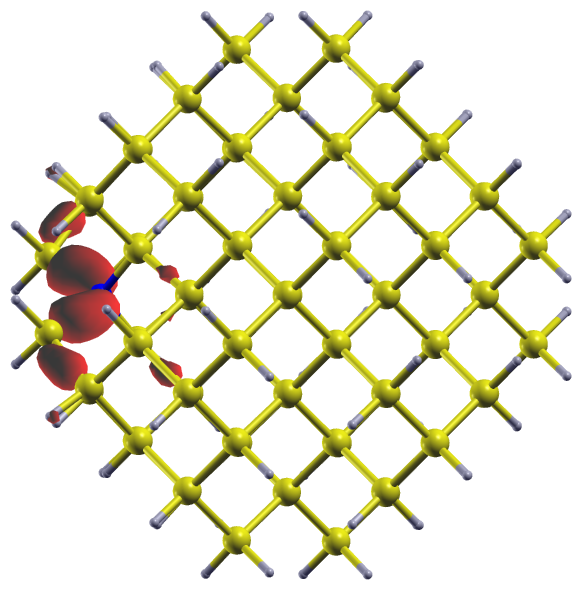
Figure 4: Charge densities for dopant level in $D=1.4$ nm nanocrystal for (left to right) P center, P surface, B center, and B surface configurations. The isosurface is plotted at $20-25\%$ of the maximum value.

For the P dopant, when P is in the center of the crystal, the IP hardly changes with nanocrystal size (the red line that tracks the $IP_{d}$ trend is nearly flat). This can be attributed to the strong electron-impurity interaction in the confined system that gives rise to the localized defect state.(Melnikov and Chelikowsky, 2004) The size dependence of the activation energy is therefore almost entirely due to the confinement of the LUMO in the undoped system. We note a tendency for the activation energy to decrease slightly when the dopant moves to the surface. A possible explanation for this is when the dopant is placed near the surface, its wave function becomes more distorted and less symmetrical, reducing its Coulomb binding energy and therefore its $IP_{d}$. Calculated and experimentally measured values of the hyperfine splitting parameter in P-doped structures support this interpretation.(Chan et al., 2008; Fujii et al., 2002)

The B dopants can be interpreted with a similar analysis. Because the dopant level is also localized and does not vary much with crystal size, the trend in the activation energy is mostly governed by the confinement of the $IP_{u}$ in the undoped system. However, structural relaxation plays a greater role due to the smaller size of the B atom (see Ref. Ossicini et al., 2006 and Supplementary Material). Activation energies for the B dopants tend to be higher when the dopant is near the surface. This likely comes about due to structural relaxation effects and spin splitting. Spin splitting occurs because the bond lengths to the neighboring Si atoms are not evenly distributed around the dopant atom. When B is in the center, its bonds to the neighboring silicons are almost equivalent. When B is near the surface, the bonds to the outer Si atoms contract more than the bonds to the inner Si atoms. This uneven distribution contributes to increased spin splitting which raises the energy level for the dopant. For example, in the $D=1$ nm NC, the spin splitting value is $2.842$ eV when B is at the center and $3.026$ eV when B is near the surface. This interpretation follows that in another DFT study on B-doped Si NCs.(Ni et al., 2017)

IV Conclusions

We applied the stochastic BNL approach to study dopant activation energies for P- and B- doped Si nanocrystals with up to $1600$ electrons. The stochastic approach reduces the scaling of the exact exchange from quadratic to linear, enabling its application to experimentally relevant system sizes. We find excellent agreement with $\Delta\text{SCF}$ and good agreement with stochastic GW for dopant activation energies using a single range-parameter ($\gamma$) for the stochastic BNL functional. The difference for stochastic GW could be influenced by the underlying LDA starting point, which erroneously predicts shallow dopant levels. One of the key findings is that shallow dopants in the bulk become deep dopants under confinement. This has been observed in previous studies using $\Delta$SCF at the LDA level, but we can finally use stochastic BNL to validate these results at the hybrid functional level.

This study is further significant in that it provides a way to calculate a self-consistent solution with a quasiparticle model Hamiltonian at a low computational cost. This quasiparticle Hamiltonian, which is not obtainable through traditional GW methods, can be further processed and used with methods like time-dependent DFT and stochastic BSE(Rabani et al., 2015) to describe optical excitations for system sizes and complexities beyond current limitations.