The CARMENES search for exoplanets around M dwarfs

We present the discovery and characterisation of two transiting planets observed by the Transiting Exoplanet Survey Satellite (TESS) orbiting the nearby ($d_{\star}$$\approx$ $22$ pc), bright ($J\approx 9$ mag) M3.5 dwarf LTT 3780 (TOI–732). We confirm both planets and their association with LTT 3780 via ground-based photometry and determine their masses using precise radial velocities measured with the CARMENES spectrograph. Precise stellar parameters determined from CARMENES high-resolution spectra confirm that LTT 3780 is a mid-M dwarf with an effective temperature of $T_{\mathrm{eff}}$= ${3360}\,{\pm}\,{51}$ $\mathrm{K}$, a surface gravity of $\log\,g_{\star}$= ${4.81}\,{\pm}\,{0.04}$ $\mathrm{(cgs)}$, and an iron abundance of $\mathrm{[Fe/H]}$= ${0.09}\,{\pm}\,{0.16}$ $\mathrm{dex}$, with an inferred mass of $M_{\star}$= ${0.379}\,{\pm}\,{0.016}$ $\mathrm{M_{\odot}}$ and a radius of $R_{\star}$= ${0.382}\,{\pm}\,{0.012}$ $\mathrm{R_{\odot}}$. The ultra-short-period planet LTT 3780 b ($P_{\mathrm{b}}$ = $0.77$ d) with a radius of $1.35^{+0.06}_{-0.06}$ $\mathrm{R_{\oplus}}$, a mass of $2.34^{+0.24}_{-0.23}$ $\mathrm{M_{\oplus}}$, and a bulk density of $5.24^{+0.94}_{-0.81}$ ${\rm g\,cm^{-3}}$ joins the population of Earth-size planets with rocky, terrestrial composition. The outer planet, LTT 3780 c, with an orbital period of $12.25$ d, radius of $2.42^{+0.10}_{-0.10}$ $\mathrm{R_{\oplus}}$, mass of $6.29^{+0.63}_{-0.61}$ $\mathrm{M_{\oplus}}$, and mean density of $2.45^{+0.44}_{-0.37}$ ${\rm g\,cm^{-3}}$ belongs to the population of dense sub-Neptunes. With the two planets located on opposite sides of the radius gap, this planetary system is an excellent target for testing planetary formation, evolution, and atmospheric models. In particular, LTT 3780 c is an ideal object for atmospheric studies with the James Webb Space Telescope.

1 Introduction

In a sequence of space-based transit surveys that commenced with the CoRoT mission (Auvergne et al., 2009) and continued with Kepler (Borucki et al., 2010) and K2 (Howell et al., 2014), the Transiting Exoplanet Survey Satellite (TESS; Ricker et al., 2015) is the first to cover nearly the entire sky in a search for transiting planets. This includes 2 min short-cadence monitoring of almost all M dwarfs brighter than 15 mag in the TESS bandpass. Based on Kepler results, Dressing & Charbonneau (2013) showed that planets with radii below 4 $\mathrm{R_{\oplus}}$ are almost the only type of planets orbiting M dwarfs. Planetary systems around bright TESS red dwarfs are therefore optimal laboratories for testing formation, evolution, and interior models of small planets ($R_{p}$ $\in$ 1–4 $\mathrm{R_{\oplus}}$) that have no known counterparts in the Solar System. Detailed characterisation of small planets orbiting bright M dwarfs also allows optimal candidates to be selected for future in-depth atmospheric studies (see e.g. Snellen et al., 2013; Batalha et al., 2018).

As was shown by Fulton et al. (2017) and Fulton & Petigura (2018), the radius distribution of small, close-in planets (with orbital periods $P<$ 100 d) has a bi-modal structure with a gap around 1.7 $\mathrm{R_{\oplus}}$ that separates the two main classes of small planets: presumably rocky super-Earths with radii centred at 1.2 $\mathrm{R_{\oplus}}$, and gas-dominated sub-Neptunes with radii centred at 2.4 $\mathrm{R_{\oplus}}$. For planets orbiting the same star, and hence exposed to the same irradiation, differences in the planetary bulk densities and atmospheric structures could then be mainly explained by differences in their masses and orbital distance. Planetary systems with two or more close-in, small planets located below and above the radius gap are therefore especially interesting for studying the formation, evolution, and atmospheric composition of small planets. So far only a few such systems have been characterised in terms of precise radii measured with space-based transit telescopes and masses determined via high-precision radial velocity (RV) measurements. These systems are: Kepler-10 bc (Dumusque et al., 2014), K2-106 bc (Sinukoff et al., 2017; Guenther et al., 2017), HD 3167 bc (K2-96 bc; Christiansen et al., 2017; Gandolfi et al., 2017), GJ 9827 bcd (K2-135 bcd; Niraula et al., 2017; Prieto-Arranz et al., 2018), K2-138 bcdef (Christiansen et al., 2018; Lopez et al., 2019), HD 15337 bc (TOI-402 bc; Gandolfi et al., 2019; Dumusque et al., 2019), and K2-36 bc (Damasso et al., 2019).

Here, we present the discovery of two transiting TESS planets straddling the radius gap around the nearby, bright M dwarf LTT 3780. Given the brightness of the host star, these planets are suitable for detailed atmospheric characterisation with future ground- and space-based facilities. The paper is structured as follows: Section 2 presents the analysis of TESS photometry used for the discovery of planets around LTT 3780. In Section 3, ground-based observations of LTT 3780 are presented, including seeing-limited transit photometry, high-resolution imaging, and high-resolution spectroscopy with CARMENES. Detailed analyses of the stellar properties of LTT 3780 are presented in Section 4, while Section 5 presents the joint analysis of all available data and the derived planetary properties. Finally, a discussion and conclusions are presented in Sections 6 and  7.

2 TESS photometry

2.1 Space-based observations

LTT 3780 (TOI–732, TIC 36724087) was observed by TESS in short cadence mode (2-min integrations) during cycle 1, sector 9 (camera #1, CCD #1) between 28 February and 25 March 2019, and it is expected to be observed again during the first year of the extended mission (cycle 3), sector 35 (camera #1) between 9 February and 7 March 2021. In total, 21.736 days of science data were collected for LTT 3780. The 1.182-day gap in the TESS photometry between $\mathrm{BJD_{TDB}}$ = 2458555.54677 and $\mathrm{BJD_{TDB}}$ = 2458556.72869 was caused by the data download during perigee passage. Data collected between $\mathrm{BJD_{TDB}}$ = 2458543.22185 and $\mathrm{BJD_{TDB}}$ = 2458544.43991 (1.218 day) and between $\mathrm{BJD_{TDB}}$ = 2458556.72869 and $\mathrm{BJD_{TDB}}$ = 2458557.85228 (1.123 day) were excluded from the light curves of all targets on Camera #1 CCD #1 because of the strong scattered light at the beginning of orbits 25 and 26 that was problematic for systematic error correction and the subsequent transiting planet search.

2.2 Transit search

We downloaded from the Mikulski Archive for Space Telescopes (MAST) the corresponding TESS light curve of LTT 3780 produced by the Science Processing Operations Center (SPOC; Jenkins et al., 2016) at the NASA Ames Research Center. For this target, SPOC provided simple aperture photometry (SAP; Twicken et al., 2010; Morris et al., 2017) and systematics-corrected photometry, a procedure consisting of an adaptation of the Kepler Pre-search Data Conditioning algorithm (PDC; Smith et al., 2012; Stumpe et al., 2012, 2014) to TESS. The SPOC light curves generated by both methods are shown in the first two panels of Fig. 1.

Additionally, we retrieved the TESS target pixel file (TPF) from MAST and performed a custom selection of pixels to build the optimal aperture that maximises the transit signals in the light curve (see Section 2.3). Following the methods described in Hidalgo et al. (2020), we used our own analysis pipeline based on the everest pipeline (Luger et al., 2016, 2018), which applies the pixel level decorrelation (PLD) technique (Deming et al., 2015) to extract from the raw light curve a final, flattened version (see bottom panel in Fig. 1). To detect possible transit events, we used the box-fitting least squares (BLS) algorithm (Kovács et al., 2002) on the flattened light curve to search for periodic signals. Once a signal was detected, we modelled the transit with batman (Kreidberg, 2015) and removed it from the light curve. We iteratively used this procedure until no further signals were detected. We found two periodic signals at $0.7685\pm 0.0007$ and $12.254\pm 0.007$ days, respectively. These signals are associated with TESS objects of interest (TOIs) 732.01 and 732.02. Alerts were issued for the TOIs based on SPOC Data Validation reports (Jenkins et al., 2010; Twicken et al., 2018; Li et al., 2019), which identified the two transit signatures.

2.3 Limits on photometric contamination

The common proper motion companion to LTT 3780, namely LP~729–55 (TIC 36724086, label #2 in Fig. 2; see Section 4.1), was located just outside the aperture mask used to extract the light curve of LTT 3780. However, another close-in star, TIC 36724077 (Gaia DR2 3767281536635597568, 2MASS J10183398–1143258), separated by 23.42″ from LTT 3780 and 3.4 mag fainter than LTT 3780 in the broad Gaia $G$ band (label #3 in Fig. 2) was located within the aperture mask. Taking advantage of the similar spectral coverage of the Gaia $G_{R_{P}}$ band (630–1050 nm) and TESS band (600–1000 nm), we estimated the dilution factor for TESS, $D_{TESS}=1/(1+F_{C}/F_{T})$, based on integrated Gaia $R_{P}$ mean fluxes of the contaminant star, TIC 36724077 ($F_{C}=10476.9\pm 17.5$), and LTT 3780 itself ($F_{T}=437973\pm 662$), to be $D_{TESS}=0.9766$. This means that TIC 36724077 dilutes the transit depths in the light curve of LTT 3780 and hence decreases the apparent planet–star radius ratios. Therefore, to measure the unaffected radii of planets we fitted for the dilution factor in TESS photometry in the combined transit and RV analysis (see Section 5.2).

2.4 A third single-transit planet?

While we find no statistically significant signals for additional transits, once the two planets are removed, the light curves present two dips that might correspond to single-transit events, namely at 2458559.796 and 2458566.124 BJD. The presence and shape of these potential transits vary depending on the use of MAST flattened light curves or our custom flattening procedure, and in both cases the transit shape is not clear, so we cannot claim the presence of a third transiting planet in the system. The analysis of future TESS re-observations of this object should help solve this ambiguity.

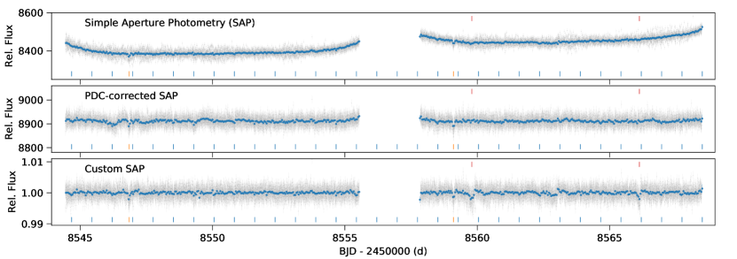
Figure 1: TESS data of LTT 3780. Top panel: Simple-aperture photometry from SPOC pipeline. Middle panel: PDC-corrected photometry from SPOC pipeline. Bottom panel: Custom-aperture photometry as in Hidalgo et al. (2020). Blue and orange ticks below the light curve mark the transits of the candidates TOI–732.01 (blue) and TOI–732.02 (orange). Red ticks above the light curves mark two dips that might correspond to single-transit events.

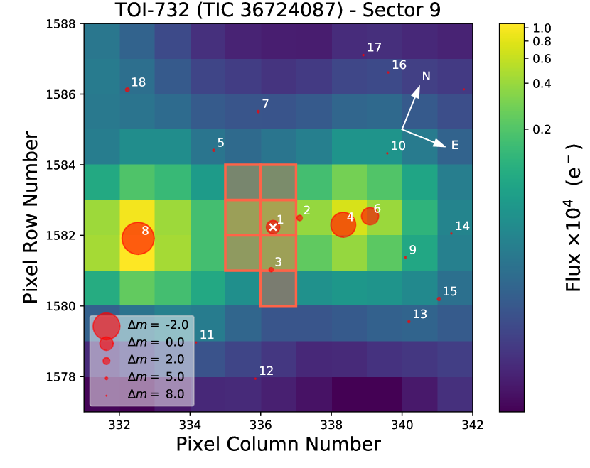
Figure 2: TESS image of LTT 3780 in Sector 9 (created with tpfplotter, Aller et al. 2019). The electron counts are colour-coded. The red bordered pixels are used in SAP. The size of the red circles indicates the TESS magnitudes of all nearby stars and LTT 3780 (label #1 with the ”$\times$”). Positions are corrected for proper motions between Gaia DR2 epoch (2015.5) and TESS Sector 9 epoch (2019.2). The TESS pixel scale is 21″approximately.

3 Ground-based follow-up observations

3.1 Seeing-limited transit photometry

We acquired ground-based time-series follow-up photometry of LTT 3780 as part of the TESS Follow-up Observing Program (TFOP) to attempt to ($i$) rule out nearby eclipsing binaries as potential sources of the TESS detection, ($ii$) detect the transit-like event on target to confirm the event depth and thus the TESS photometric deblending factor, ($iii$) refine the TESS ephemeris, ($iv$) provide additional epochs of transit centre time measurements to supplement the transit timing variation analysis, and ($v$) place constraints on transit depth differences across optical filter bands. We used the TESS Transit Finder, which is a customised version of the Tapir software package (Jensen, 2013), to schedule our transit observations. Unless otherwise noted, the photometric data were extracted using the AstroImageJ software package (Collins et al., 2017). A summary of the photometric ground-based observations is shown in Table 1.

Table 1: Observing log of ground-based photometric observations.

Telescope	Planet	Date	Filter	Coverage
TCS	.01	2019-12-28	$g$ $r$ $i$ $z_{s}$	100 %
	.01	2020-01-24	$g$ $r$ $i$ $z_{s}$	100 %
	.01	2020-01-27	$g$ $r$ $i$ $z_{s}$	100 %
	.01	2020-01-30	$g$ $r$ $i$ $z_{s}$	100 %
	.02	2019-12-10	$g$ $r$ $i$ $z_{s}$	80 %
	.02	2020-01-28	$g$ $r$ $i$ $z_{s}$	100 %
SNO-T150	.02	2019-12-10	$V$ $R$	100 %
TRAPPIST-North	.02	2019-12-10	$z$	100 %
LCO-CTIO	.01	2019-06-09	$z_{s}$	100 %
	.01	2019-06-16	$z_{s}$	100 %
LCO-SAAO	.01	2019-06-17	$g_{p}$ $z_{s}$	100 %
LCO-SSO	.02	2020-01-04	$B$	100 %
OAA	.01	2020-02-01	$Ic$	100 %

3.1.1 Las Cumbres Observatory network

In total, four transits of the LTT 3780 system where observed with the SINISTRO CCDs operating in the 1m telescopes of the Las Cumbres Observatory (LCOGT) network (Brown et al., 2013). For LTT 3780 b, two transits were observed from the Cerro Tololo Inter-American Observatory (CTIO) site using the $z_{s}$ filter on 9 and 16 June 2019. Exposure times were set to 45 s and 70 s, respectively, and an optimum aperture of 15.0 pix (5.83 ″). A third transit was observed using the $g_{p}$ and $z_{s}$ filters from the South Africa Astronomical Observatory (SAAO) site on 17 June 2019 with exposure times of 140 s and the optimum apertures of 12.0 pix (4.67 ″) and 15.0 pix (5.83 ″) for filters $g_{p}$ and $z_{s}$, respectively. For LTT 3780 c, one transit observation was performed from Siding Spring Observatory (SSO) on 4 January 2020, using the $B$ filter, an exposure time of 140 s and an optimum aperture of 7 pix (2.66 ″).

3.1.2 TRAPPIST-North

TRAPPIST-North at Oukaimeden Observatory in Morocco is a 60 cm Ritchey-Chrétien telescope, which has a thermo-electrically cooled 2k$\times$2k Andor iKon-L BEX2DD CCD camera with a field of view of 20′$\times$20′and pixel scale of 0.60 ″ pix^-1 (Jehin et al., 2011; Barkaoui et al., 2019). We carried out a full-transit observation of TOI–732.02 on 10 December 2019 using a $z$ filter with an exposure time of 10 s. We took 507 images and performed aperture photometry with an optimum aperture of 11 pixels (6.6″) and a point spread function (PSF) full width half maximum (FWHM) of 3.7″. We confirmed the event on the target star with a depth of $\sim$3.2 ppt (parts per thousand) and occurring about 1 h sooner with respect to the predicted ingress, but still within the expected uncertainty from an ephemeris derived from the TESS data only. We cleared all the stars of eclipsing binaries within the 2.5′around the target star.

3.1.3 Sierra Nevada Observatory-T150 multicolour photometry

T150 at Sierra Nevada Observatory (SNO) in Granada (Spain) is a 150 cm Ritchey-Chrétien telescope equipped with another thermo-electrically cooled 2k$\times$2k Andor iKon-L BEX2DD CCD camera with a field of view of 7.9′$\times$7.9′and pixel scale of 0.23 ″ pix^-1. We carried out a full-transit observation of TOI–732.02 on 10 December 2019 with $R$ and $V$ filters (placed on a filter wheel) with an exposure time of 20 s and 60 s, respectively. We took 125 images (2$\times$2 binning) in both filters, and performed aperture photometry with an optimum aperture of 10 pix (4.6″) in $R$ and 11 pix (5.0″) in $V$ and a PSF FWHM of 2.3 ″and 2.7″, respectively. We confirmed the event on the target star in both filters, with similar depth of $\sim$3.2 ppt and also about 1 h earlier than the predicted ingress.

3.1.4 Observatori Astronòmic Albanyà

Additional photometric observations of TOI–732.01 were acquired on 1 February 2020 with the 0.4 m telescope at the Observatori Astronòmic Albanyà (OAA), in Catalonia, Spain. The host star was observed for 391.7 min with a Cousins $I_{c}$ filter and a Moravian G4-9000 camera with a field of view of 3056(H) $\times$ 3056(V) pixels covering 36.8 ′. We performed aperture photometry with an optimum aperture of 14 pix (20.3″) and a PSF FWHM of 13.0 ″. We confirmed the event on the target with depth of $\sim$2.9 ppt and occurring about 15 minutes later than the predicted ingress (within the expected uncertainty of the ephemeris derived from the TESS data only).

3.1.5 Telescopio Carlos Sánchez/MuSCAT2 multicolour photometry

We observed four transits of TOI–732.01 and two transits of TOI–732.02 with the MuSCAT2 multi-colour imager (Narita et al., 2019) installed at the Telescopio Carlos Sánchez (TCS), located at the Teide Observatory in Tenerife, Spain. The instrument carries out high-precision, simultaneous photometry in four colours ($g$, $r$, $i$, $z_{\mathrm{s}}$) with a pixel scale of 0.44″ pix^-1. Observations were reduced with a dedicated MuSCAT2 pipeline (see Parviainen et al., 2019, for details).

The exposure times varied from passband to passband and night to night depending on observing conditions and the observer’s judgement. The shortest exposure times were of the order of 5 s, and the longest of 60 s. The aperture photometry was performed with an the optimum apertures of 5–6″, depending on the seeing and possible defocusing at a given observing night. The reduction included an initial detrending, after which all the light curves were down-sampled to a 1 min cadence. The covariates used in the detrending were also down-sampled and stored, and used in the linear baseline model in the final joint light curve and RV modelling.

3.2 Other light curves from public databases

We compiled photometric series obtained by long-time baseline automated surveys as in Díez Alonso et al. (2019). We were only able to retrieve data from the All-Sky Automated Survey for Supernovae (ASAS-SN; Kochanek et al., 2017), but not from other public catalogues, such as the All-Sky Automated Survey (ASAS; Pojmanski, 2002), Northern Sky Variability Survey (NSVS; Woźniak et al., 2004), The MEarth Project (Charbonneau et al., 2008), the Catalina surveys (Drake et al., 2014), or the Hungarian Automated Telescope Network (Bakos et al., 2004). The ASAS-SN dataset comprises 220 observations spanning about 2000 d in $V$ band.

Additionally, LTT 3780 is a candidate of the Super-Wide Angle Search for Planets (SuperWASP; Pollacco et al., 2006). SuperWASP acquired more than 40 000 photometric observations using a broad-band optical filter spanning two consecutive seasons from January to June 2013, and January to June 2014. For our search to detect long-term photometric modulations associated with the stellar rotation, we binned the data to one-day intervals, resulting in 191 epochs.

3.3 High-contrast imaging

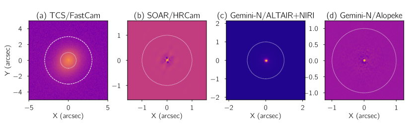
Figure 3: High-spatial-resolution images of LTT 3780 from TCS/FastCam lucky imaging (panel a), SOAR/HRCam speckle imaging (panel b), Gemini North/ALTAIR+NIRI (panel c), and Gemini North/‘Alopeke at 832 nm (panel d). The dotted circle corresponds to 1″and the dashed circle to 3″separation. North is up and east is left.

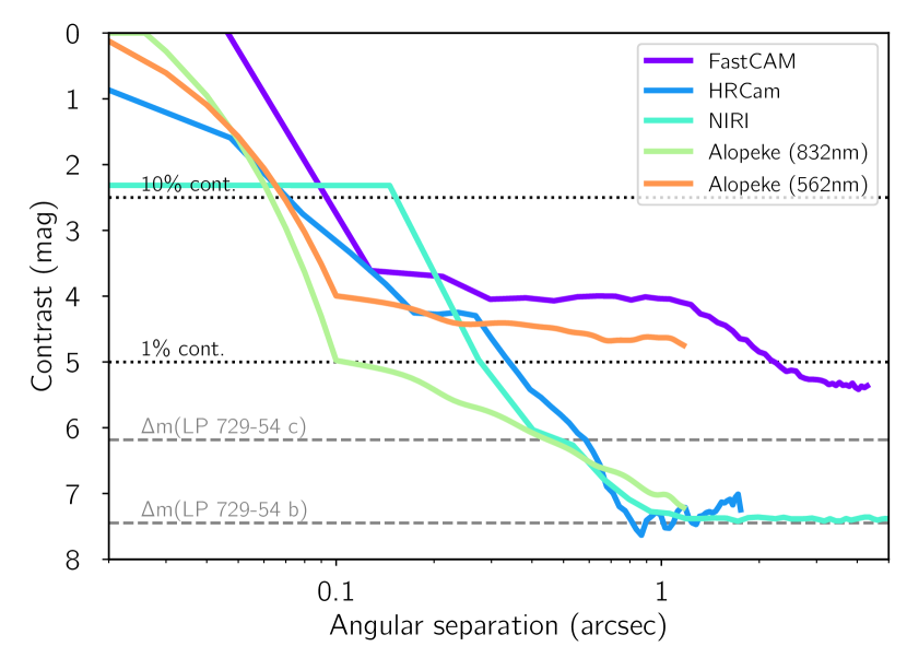
Figure 4: Sensitivity curves (5$\sigma$ limits) for all five high-spatial resolution images used in this work. The 1 % and 10 % contamination levels are marked as black dotted horizontal lines and the maximum magnitude contrast that a blended binary could have to mimic the transit depth of the two planets in the system are marked as grey dashed horizontal lines.

The presence of an unknown star within the same TESS pixel as the target can result in under-estimated planetary radii, caused by the additional light diluting the transit depth. These unaccounted stars could also potentially be the source of astrophysical false positives, although this was found to be unlikely for multi-planet transiting systems (Lissauer et al., 2012). To search for close-in companion stars (bound or unbound to the target star), and to estimate the potential contamination factor from such sources, we used high-contrast images of LTT 3780 acquired with four instruments: (1) FastCam (Oscoz et al., 2008) mounted on the 1.5 m TCS (see Section 3.1.5); (2) HRCam (Tokovinin, 2018) installed on the 4.1 m Southern Astrophysical Research (SOAR) telescope at CTIO; (3) ‘Alopeke, a high-resolution speckle interferometry instrument on the 8 m Frederick C. Gillett Gemini North telescope at Gemini North Observatory, Hawai’i, USA; and (4) Near InfraRed Imager and spectrograph (NIRI, Hodapp et al., 2003) coupled with the adaptive optics (AO) system facility, ALTAIR, mounted also on Gemini North.

3.3.1 TCS/FastCam lucky imaging

LTT 3780 was observed with the FastCam instrument on 22 May 2014 in the $I$ band as part of our high-resolution imaging campaign to identify and characterise the binary content of the CARMENES sample of M dwarfs (Cortés-Contreras et al., 2017). FastCam is a lucky imaging camera mounted on TCS and is equipped with a high readout speed and sub-electron noise L3CCD Andor 512$\times$512 detector, with a pixel size of 0.0425 ″, which provides a field of view of 21.2″$\times$ 21.2″. Ten blocks of 1 000 individual frames of 50 ms exposure time were obtained for this target. Data were processed using a dedicated pipeline developed by the Universidad Politécnica de Cartagena group (see Labadie et al., 2010; Jódar et al., 2013), which includes bias correction, the alignment and combination of images, and the selection of the best-quality images using the pixel position and value of the brightest speckle. Figure 3 (panel a) shows the FastCam image resulting from selecting the 50% best-quality images of the first 4 000 frames. The corresponding 5$\sigma$ detection sensitivity curve is shown in Fig. 4. No additional source is detected with $\delta\,I<$ 4 mag down to the resolution limit of the telescope ($\sim$ 0.15 ″).

3.3.2 SOAR/HRCam speckle imaging

LTT 3780 was observed with SOAR/HRCam speckle imaging on 12 December 2019 (UT) in $I$ band, a similar visible bandpass to that of TESS, to search for nearby sources. Further details of observations are available in Ziegler et al. (2020). The region within 3 ″ of LTT 3780 was found to be devoid of nearby stars (see Fig. 3, panel b) within the 5$\sigma$ detection sensitivity of the observation, which is shown in Fig. 4.

3.3.3 Gemini North/‘Alopeke speckle imaging

LTT 3780 was observed on 17 February 2020 (UT) at Gemini North with ‘Alopeke, the high-resolution speckle interferometry instrument. The star was observed simultaneously in two bandpasses centred at 562 nm and 832 nm (the latter is shown in panel d of Fig. 3). The resulting contrast curves are shown in Fig. 4, from which we deduced that LTT 3780 does not have any close companion. At the distance of LTT 3780, our inner working angle is 0.37 au at 562 nm and 0.62 au at 832 nm, respectively, and our field of view ($r$ = 1.25″) extends out to 28 au from the star. Given that LTT 3780 is an M3.5 V star, our contrast curves eliminate any companion object down to the M–L boundary in luminosity.

3.3.4 Gemini-North/NIRI+ALTAIR AO imaging

On 25 November 2019 (UT) we acquired AO images of LTT 3780 with the Gemini North/NIRI+ALTAIR using the Br$\gamma$ filter (Gemini-North ID G0218) centred at 2.17 $\mathrm{\mu m}$. We collected nine images, each with an integration time of 2.2 s, and dithered the telescope between each exposure. Images were reduced following standard procedures, that is, correction for bad pixels, flat-fielding, subtraction of a sky background constructed from the dithered images, alignment of the star between frames, and co-addition of data. The Gemini North/NIRI+ALTAIR AO image of LTT 3780 (see panel c of Fig. 3) revealed no close-in companions and the star appeared single to the limit of our resolution. Fig. 4 presents the 5$\sigma$ contrast curve as a function of the angular separation from LTT 3780. We calculated the sensitivity to faint companions as a function of radius by injecting synthetic point spread functions at a range of magnitudes into the data, and measuring the significance at which they could be recovered. The data were of high quality, and we were sensitive to companions 5.0 mag fainter than the target at just 270 mas, and 7.4 mag fainter than the target at separations greater than $\sim$1″.

3.4 High-resolution spectroscopy

3.4.1 3.5 m Calar Alto/CARMENES

We obtained 52 high-resolution spectra of LTT 3780 between 27 December 2019 (UT) and 19 February 2020 (UT) with the CARMENES instrument (Quirrenbach et al., 2014, 2018) mounted on the 3.5 m telescope at the Calar Alto Observatory, Almería, Spain, as part of the guaranteed time observation program to search for exoplanets around M dwarfs (Reiners et al., 2018). The CARMENES spectrograph has two channels, the visible (VIS) one covering the spectral range $0.52$–$0.96\text{\,}\mathrm{\SIUnitSymbolMicro m}$ and a near-infrared (NIR) channel covering the spectral range $0.96$–$1.71\text{\,}\mathrm{\SIUnitSymbolMicro m}$.

Relative radial-velocity values, chromatic index (CRX), differential line width (dLW), and H$\alpha$ index values were obtained using serval (Zechmeister et al., 2018). For each spectrum, we also computed the cross-correlation function (CCF) and its FWHM, contrast (CTR) and bisector velocity span (BVS) values, following Lafarga et al. (2020). The RV measurements were corrected for barycentric motion, secular acceleration, and nightly zero-points. For more details, see Trifonov et al. (2018) and Kaminski et al. (2018).

3.4.2 Subaru/IRD

We observed LTT 3780 with the InfraRed Doppler instrument (IRD, Kotani et al., 2018) behind an AO system (AO188, Hayano et al., 2010) on the Subaru 8.2 m telescope on Mauna Kea Observatories, as part of the Subaru IRD-TESS intensive follow-up project (S19A–069I). We took four spectra of LTT 3780 on 10 December 2019 (UT) and one spectrum on 13 December 2019 simultaneously with laser-frequency comb spectra. Exposure times were 480 s and a signal-to-noise ratio (S/N) at $1.0\text{\,}\mathrm{\SIUnitSymbolMicro m}$ was $\sim$100 for the four spectra, but the S/N was only $\sim$15 for the last one owing to thick clouds. We reduced the raw IRD frames of LTT 3780 using the echelle package of iraf for flat-fielding, scattered-light subtraction, aperture tracing, and wavelength calibration with the Th-Ar lamp spectra. For RV measurements requiring a more precise wavelength calibration, the wavelength was re-calibrated based on the emission lines of the combined laser frequency comb, which was injected simultaneously into both stellar and reference fibres during instrument calibrations. We injected these reduced spectra into the RV analysis pipeline for Subaru/IRD (Hirano et al., 2020) and attempted to reproduce the intrinsic stellar template spectrum from all the observed spectra with instrumental profile deconvolution and telluric removal. Radial velocities were measured with respect to that template by forward-modelling of the observed individual spectral segments (each spanning 0.7–1.0 nm). We found that the RV precision for the first-night spectra was typically 2.4 m s^-1, while that of the second night was $\approx$19 m s^-1 due to the low quality of the spectrum. We therefore discarded the latter measurement from the final analysis.

3.4.3 NASA Infrared Telescope Facility/iSHELL

We obtained 77 five-minute spectra during seven nights for LP 729-54 spanning 28 days from January to February 2020 with the iSHELL spectrometer on the NASA Infrared Telescope Facility (IRTF, Rayner et al., 2016). Five-minute exposures were repeated 8-15 times within a night to reach a cumulative photon signal-to-noise ratio per spectral pixel at about $2.2\,\mu$m (at the approximate centre of the blaze for the middle order) varying from 152 to 205 to achieve a per-night RV precision of 6–10 m s^-1. Spectra were reduced and RVs extracted using the methods outlined in Cale et al. (2019).

Due to the limited barycentre sampling of the iSHELL observations over the small observing window, the underlying stellar spectrum could not be well-isolated from other spectral features (namely tellurics). Therefore, a synthetic stellar spectrum was used to compute the RVs instead of deriving a more robust stellar template from the observations themselves. The overall RV scatter is consequently larger than expected given the S/N and RV information content of the observations. Two outliers (first and fourth night) were disregarded in the analysis, which can be recovered in the future with additional observations at different barycentre velocities.

The radial velocities collected with 3.5 m Calar Alto/CARMENES, Subaru/IRD and IRTF/iSHELL instruments and their uncertainties are listed in Table 4.

4 Stellar parameters

Table 2: Stellar parameters of LTT 3780.

Parameter	Value	Reference
Name and identifiers
Name	LTT 3470	Luyten (1957)
	G 162–44	Giclas et al. (1971)
Karmn	J10185–117	Caballero et al. (2016)
TOI	732	TESS Alerts
TIC	36724087	Stassun et al. (2018)
Coordinates and spectral type
$\alpha$ (J2015.5)	10:18:34.77	Gaia DR2
$\delta$ (J2015.5)	–11:43:04.1	Gaia DR2
Sp. type	M3.5 V	Reid et al. (2003)
Magnitudes
z§ $B$ [mag]	$14.68\pm 0.04$	UCAC4
$g$ [mag]	$13.84\pm 0.05$	UCAC4
$G_{BP}$ [mag]	$13.352\pm 0.004$	Gaia DR2
$V$ [mag]	$13.14\pm 0.04$	UCAC4
$r$ [mag]	$12.55\pm 0.05$	UCAC4
$G$ [mag]	$11.8465\pm 0.0005$	Gaia DR2
$i$ [mag]	$11.09\pm 0.08$	UCAC4
$G_{RP}$ [mag]	$10.6583\pm 0.0016$	Gaia DR2
$J$ [mag]	$9.01\pm 0.03$	2MASS
$H$ [mag]	$8.44\pm 0.06$	2MASS
$K_{s}$ [mag]	$8.20\pm 0.02$	2MASS
$W1$ [mag]	$8.04\pm 0.02$	AllWISE
$W2$ [mag]	$7.880\pm 0.019$	AllWISE
$W3$ [mag]	$7.771\pm 0.019$	AllWISE
$W4$ [mag]	$7.58\pm 0.17$	AllWISE
Parallax and kinematics
$\pi$ [mas]	$45.46\pm 0.08$	Gaia DR2
$d$ [pc]	$22.00\pm 0.04$	Gaia DR2
$\mu_{\alpha}\cos\delta$ [$\mathrm{mas\,yr^{-1}}$]	$-341.411\pm 0.11$	Gaia DR2
$\mu_{\delta}$ [$\mathrm{mas\,yr^{-1}}$]	$-247.87\pm 0.10$	Gaia DR2
$V_{r}$ [$\mathrm{km\,s^{-1}}]$	$-0.44\pm 0.09$	Jeffers et al. (2018)
$U$ [$\mathrm{km\,s^{-1}}]$	$-14.89\pm 0.06$	This work
$V$ [$\mathrm{km\,s^{-1}}]$	$-22.00\pm 0.08$	This work
$W$ [$\mathrm{km\,s^{-1}}]$	$-35.08\pm 0.07$	This work
Galactic population	Thin disc	This work
Photospheric parameters
$T_{\mathrm{eff}}$ [K]	$3360\pm 51$	This work
$\log g$	$4.81\pm 0.04$	This work
[Fe/H]	$+0.09\pm 0.16$	This work
$v\sin i_{\star}$ [$\mathrm{km\,s^{-1}}$]	$<3.0$	Jeffers et al. (2018)
Physical parameters
$L$ [$10^{-4}\,L_{\odot}$]	$167\pm 3$	This work
$R$ [$R_{\odot}$]	$0.382\pm 0.012$	This work
$M$ [$M_{\odot}$]	$0.379\pm 0.016$	This work
$\rho$ [$\mathrm{g\,cm^{-3}}$]	$9.6\pm 1.0$	This work

2MASS: Skrutskie et al. (2006); AllWISE: Cutri & et al. (2013); Gaia DR2: Gaia Collaboration et al. (2018); UCAC4: Zacharias et al. (2013).

4.1 The stellar host and its binary system

LTT 3780 is a relatively bright ($J\,\approx\,9.0$ mag) M3.5 V star at approximately 22 pc (Gaia Collaboration et al., 2018). According to the Washington Double Star catalogue (Mason et al., 2001), it is the primary of the poorly investigated wide system LDS 3977 (Luyten, 1963). The secondary, located at angular separation $\rho$ = 15.81$\pm$0.15″ and position angle $\theta$ = 96.9$\pm$0.2 deg (at epoch J2015.5), is LP~729–55, which is about 2.1 mag fainter in the $J$ band and shares within $1\sigma$ the same parallax and proper motions as LTT 3780 (Gaia Collaboration et al., 2018). At the system heliocentric distance, $\rho$ translates into a projected physical separation of $s$ = 348$\pm$3 au. Reid et al. (2003) assigned the spectral type M3.5 V to the secondary from low-resolution spectroscopy. However, we consider that they meant the primary instead, whose spectral type agrees within 0.5 dex with that derived by Scholz et al. (2005), as well as with its effective temperature (see below). From accurate absolute magnitudes, colours, and luminosity and using various magnitude-, colour-, and luminosity-spectral type relationships available in the literature for solar-metallicity M-type stars, we estimate an m5.0$\pm$0.5 V spectral type for the common proper companion secondary LP 729–55.

4.2 Photospheric and physical parameters

The photospheric parameters of LTT 3780 were determined following Passegger et al. (2019) using improved PHOENIX-ACES (Husser et al., 2013) stellar atmosphere models, which include a new equation of state to especially account for spectral features of low-temperature stellar atmospheres, as well as new atomic and molecular line lists. Effective temperature, surface gravity, and metallicity were derived assuming $v\sin i_{\star}=2\,\mathrm{km\,s^{-1}}$ and a stellar age of 5 Gyr (see Passegger et al., 2019). The latter two values are consistent with the rotational velocity upper limit determined by Jeffers et al. (2018) and an approximate solar age from the kinematic membership in the Galactic thin disc, using the same Galactocentric space velocity computation as Cortés-Contreras (2016).

To compute the physical parameters we followed the multi-step approach of Schweitzer et al. (2019). First, we determined the luminosity $L$ by integrating the photometric stellar energy distribution collected for the CARMENES targets (Caballero et al., 2016) with the Virtual Observatory Spectral energy distribution Analyser (Bayo et al., 2008) using parallactic distances from the Gaia DR2 catalogue (Gaia Collaboration et al., 2018). We then derived the radius $R$ and mass $M$ using the Stefan–Boltzmann’s law and the empirical $M$-$R$ relation presented in Schweitzer et al. (2019), respectively.

We derived an effective temperature of $T_{\rm eff}=3360\pm 51\,\mathrm{K}$, a stellar mass of $M_{\star}=0.379\pm 0.016\,\mathrm{M_{\odot}}$, and a radius of $R_{\star}=0.382\pm 0.012\,\mathrm{R_{\odot}}$, resulting in a stellar density of $\rho=9.6\pm 1.0\,\mathrm{g\,cm^{-3}}$. All derived values and additional stellar parameters can be found in Table 2.

4.3 Stellar activity and rotation period

Using the stellar radius determined in Section 4.2 and presented in Table 2 ($R_{\star}$ = ${0.382}\,{\pm}\,{0.012}$ $\mathrm{R_{\odot}}$) and the upper limit for the stellar projected rotation velocity found by Jeffers et al. (2018, $\mathit{v}_{\mathrm{rot}}\sin\,i_{\star}$ ¡ 3 $\mathrm{km\,s^{-1}}$), we calculated the stellar rotation period $P_{\mathrm{rot}}$ to be longer than 6 d, and shorter than 100 d for $\mathit{v}_{\mathrm{rot}}\sin\,i_{\star}$ ¿ 0.2 $\mathrm{km\,s^{-1}}$. We performed a search for the rotation period in the existing photometric data of LTT 3780 from the SuperWASP and ASAS-SN surveys. The ASAS-SN photometry shows no variation at the precision of the data. However, an analysis using a quasi-periodic Gaussian process (GP) suggested a 66 $\pm$ 2 d period signal in the data (see Fig. 5), albeit not with very high significance. We used the quasi-periodic GP kernel introduced by Foreman-Mackey et al. (2017) of the form

$$k_{i,j}(\tau)=\frac{B}{2+C}e^{-\tau/L}\left[\cos\left(\frac{2\pi\tau}{P_{\textnormal{rot}}}\right)+(1+C)\right]\quad,$$

where $\tau=|t_{i}-t_{j}|$ is the time-lag, $B$ and $C$ define the amplitude of the GP, $L$ is a timescale for the amplitude modulation of the GP, and $P_{\rm rot}$ is the period of the quasi-periodic modulations. For the fit, we considered that each instrument and pass band could have different values of $B$ and $C$, while $L$ and $P_{\rm rot}$ were left as common parameters. We considered wide uninformative priors for $B$, $C$ (log-uniform between $10^{-3}$ and $10^{6}$), $L$ (log-uniform between $10^{0}$ d and $10^{8}$ d), $P_{\rm rot}$ (uniform between 10 d and 100 d), and instrumental jitter (log-uniform between 10 ppm and $10^{6}$ ppm). The 3$\sigma$ upper limit implied by this latter fit is 300 ppm, which demonstrates that LTT 3780 is magnetically inactive with only very few starspots. The photometric variability can be explained by a small starspot or group of starspots not exceeding approximately 2 % of the total area of the star assuming a star-spot temperature difference of 500 K. This is in agreement with the estimate of the RV amplitude that one could expect from rotational modulation following the prescription given by (Aigrain et al., 2012). Additionally, the H$\alpha$ activity indicator shows that LTT 3780 is an inactive star (Jeffers et al., 2018). Therefore, we conclude that the imprint of stellar activity signals in the collected CARMENES RVs is probably at the level of the measurement errors.

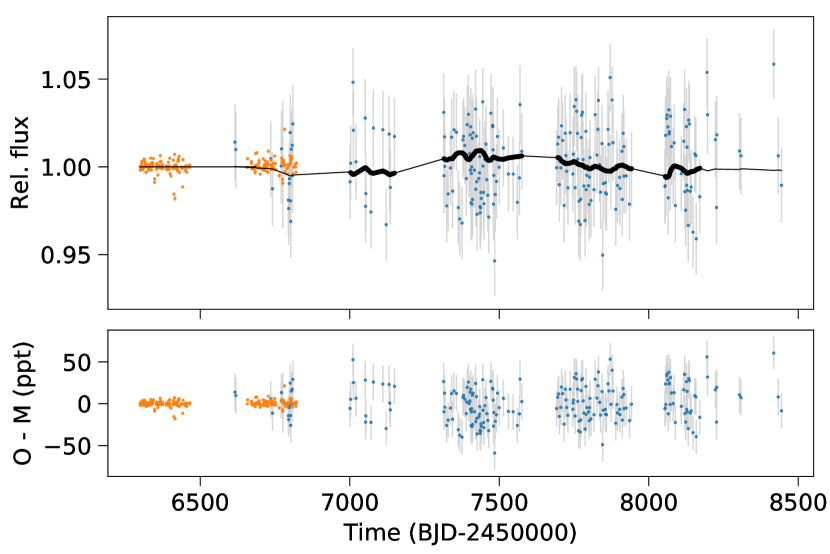
Figure 5: SuperWASP (orange) and ASAS-SN (blue) long-term photometric monitoring modelled with a quasi-periodic GP kernel defined as in Foreman-Mackey et al. (2017).

5 Analysis and results

5.1 Frequency analysis of radial velocities

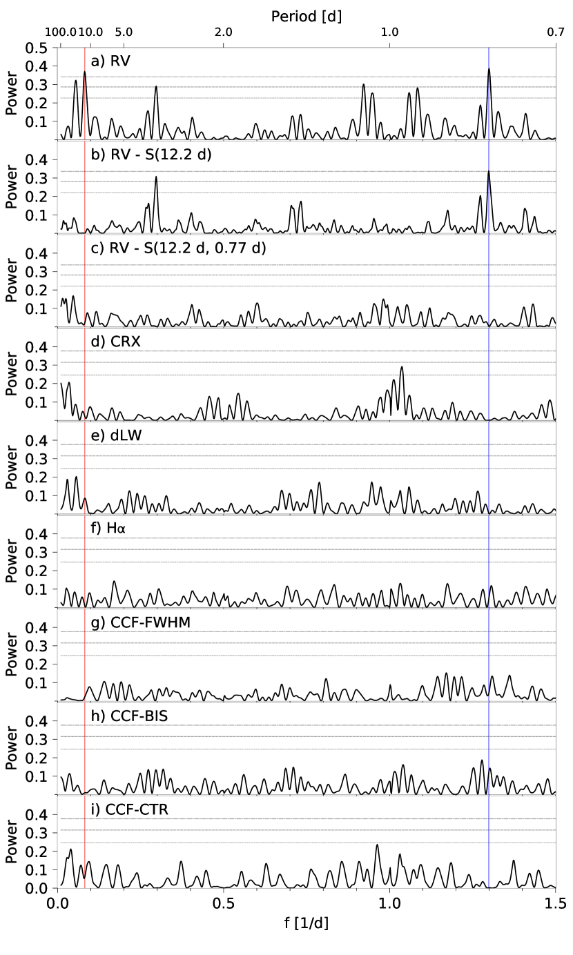
Figure 6: Generalised Lomb-Scargle periodograms for RVs of LTT 3780 (a), their residuals (b) after fitting a sinusoid with period and phase corresponding to the transiting planet TOI-732.02 ($f_{\mathrm{c}}=0.081\pm 0.002\,\mathrm{d}^{-1}$, $P_{\mathrm{c}}=12.3\pm 0.3\,\mathrm{d}$), marked in red, and their residuals (c) after fitting two sinusoids with periods and phases corresponding to the transiting planets TOI-732.02 and TOI-732.01 ($f_{\mathrm{b}}=1.298\pm 0.002\,\mathrm{d}^{-1}$, $P_{\mathrm{b}}=0.770\pm 0.001\,\mathrm{d}$), marked in blue. Panels (d–i) show periodograms of the chromatic index, differential line width, H$\alpha$ index, cross-correlation function FWHM, bisector velocity span, and contrast, all of them derived only from CARMENES observations. Horizontal lines show the theoretical FAP levels of 10 % (short-dashed line), 1 % (long-dashed line), and 0.1 % (dot-dashed line) for each panel.

In order to search for the Doppler reflex motion induced by the transiting planets and unveil the presence of possible additional signals in our time-series RV data, we performed a frequency analysis of the RV measurements and their activity indicators. We calculated the generalised Lomb-Scargle (GLS) periodograms (Zechmeister & Kürster, 2009) of the available time series and computed the theoretical 10 %, 1 %, and 0.1 % false alarm probability (FAP) levels (Fig. 6). The 70 d time baseline of the RV measurements translates into a frequency resolution of 0.01428 d^-1.

The GLS periodogram of the CARMENES data (Fig. 6a) shows two highly significant peaks ($\mathrm{FAP}<0.1\%$) at the orbital frequencies of the transiting planets, TOI–732.02 ($f_{\mathrm{c}}=0.081\pm 0.002\,\mathrm{d}^{-1}$, $P_{\mathrm{c}}=12.3\pm 0.3\,\mathrm{d}$) and TOI–732.01 ($f_{\mathrm{b}}=1.298\pm 0.002\,\mathrm{d}^{-1}$, $P_{\mathrm{b}}=0.770\pm 0.001\,\mathrm{d}$). The RV residuals after a joint fit with two circular orbits, fixed periods, and transit mid-times given by the TESS ephemerides showed no further significant peaks (Fig. 6c).

We also calculated periodograms for different activity indicators computed by SERVAL, namely the CRX (Fig. 6d), dLW (Fig. 6e), and H$\alpha$ index (Fig. 6f), and some indicators from the cross-correlation function such as FWHM, BIS, and CTR (Figs. 6g, 6h and 6i). No significant peaks were found except for some power with periods close to 1 d in CRX, which are related to the sampling of the observations. There are no peaks in any activity indicator at the frequency of the transiting planets.

5.2 Joint modelling of the light curves and RVs

We modelled the TESS light curve, the ground-based light curves, and the RVs simultaneously using PyTransit (Parviainen, 2015). The analysis followed the approach described in Parviainen et al. (2019, 2020), namely we estimated any possible flux contamination from unresolved sources inside the photometry apertures in the TESS and ground-based photometry together with the planetary parameters.

The TESS dataset included in the analysis consisted of 2.4 h windows of SAP light curves produced by the SPOC pipeline (Twicken et al., 2010; Jenkins et al., 2016; Morris et al., 2017) centred around each individual transit centre normalised to the median per-window out-of-transit flux. The SAP light curves were chosen over the PDC light curves because the trends in the light curve are dominated by the photon noise (on 2.4 h time scales), and because the PDC process removes the PDC-estimated flux contamination. The latter can introduce biases into our contamination estimation if the PDC contamination is overestimated, as we did not allow for negative contamination. By chance, the TESS dataset did not contain transits with overlapping windows. The ground-based photometry dataset included all the ground-based transit observations described in Section 3. We binned the MuSCAT2 photometry to a time cadence of one minute, but did not otherwise modify the data. The RV dataset was taken as it was, and included the 3.5 m Calar Alto/CARMENES and Subaru/IRD usable RVs described in Section 3.4.

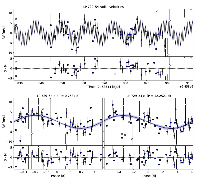
Figure 7: Top panel: CARMENES (black circles), IRD (light blue circles), and iSHELL (open circles) RV measurements along with the residuals of the median posterior joint fit model (black line) and the 68 %, 95 %, and 99 % central posterior limits (blue). Bottom panels: RVs phase-folded to the period of the two transiting planets (left: LTT 3780 b; right: LTT 3780 c).

5.2.1 Parametrisation

The joint model contained 207 free parameters, but most of them were linear coefficients used to model systematic trends in the ground-based light curves, and not of scientific interest. Of these 207 parameters, we used only 31 for describing the planets and their orbits, stellar limb darkening, and flux contamination.

Planet.

Each planet and its orbit were parametrised by the orbital period, zero epoch, true planet-star area ratio, impact parameter, two parameters describing the eccentricity and argument of periastron, and RV semi-amplitude, as detailed in Table 5. Here we made a distinction between the apparent and true planet-star area ratios. The apparent area ratio can be affected by flux contamination that leads to passband- and aperture-size-dependent variations in the apparent transit depth. However, the true area ratio stands for the uncontaminated geometric planet-star area ratio and, unlike the apparent area ratio, is independent of passband and photometry aperture size. In addition to these per-planet parameters, the stellar density was used to complete the description of the orbit.

Limb darkening.

We parametrised the stellar limb darkening with the triangular parametrisation for the quadratic limb darkening model introduced by Kipping (2013), and constrained it using the code LDTk (Parviainen & Aigrain, 2015). This yielded two parameters per passband, totalling 12 parameters for the six passbands for which we have photometric data.

Contamination.

The TESS photometry was given an unconstrained contamination factor independent of the contamination for the ground-based observations, while the contamination in the ground-based observations was modelled using a physical model introduced by Parviainen et al. (2019). This is because the TESS pixel size is significantly larger than the pixel size of the ground-based instruments used for the study, and thus we expected the contamination in the TESS data to be larger than in the ground-based photometry. In brief, the observed flux ($F_{\rm app}$), which can be used to determine the apparent planet-star radius ratio ($k_{\mathrm{app}}$) by fitting the transit model, in the light contamination model of Parviainen et al. (2019) is defined as a linear combination of the host and contaminant star fluxes (possibly from several contaminating sources). The contamination ($c$) is calculated for a set of passbands ($i$) given the passband transmission functions ($\mathcal{T}$), the effective temperatures of host ($T_{\mathrm{eff,H}}$), and contaminant stars ($T_{\mathrm{eff,C}}$), necessary to calculate relative fluxes of host ($F_{\mathrm{H}}$) and contaminant star ($F_{\mathrm{C}}$), and the level of contamination in some reference passband ($c_{0}$):

$$c_{i}=\frac{F_{\mathrm{C,i}}}{F_{\mathrm{H,i}}+F_{\mathrm{C,i}}}.$$

By combining a contamination model with a transit model and taking into account that the transit depth scales linearly with the contamination factor, the true, uncontaminated radius ratio of a transiting planet ($k_{\mathrm{true}}$) can be calculated as:

$$k_{\mathrm{true}}=k_{\mathrm{app}}/\sqrt{1-c}.$$

Trends and noise.

We chose to use a simple linear model to explain the trends in the photometry. That is, the photometry (sans transit) was explained as a dot product of a baseline coefficient vector and a covariate vector. The ground-based light curves were observed with different instruments and the photometry was reduced with different photometry pipelines. Thus, the exact set of covariates included in the baseline model varied from light curve to light curve, but the airmass, $x$- and $y$-centroid shifts, and PSF FWHM were included whenever possible. The TESS photometry was given a constant baseline fixed to unity, because adding a per-transit model would increase the number of model parameters excessively.

We also chose to use a linear baseline model rather than to model the systematics as a GP because the latter approach would have added a significant layer of complexity to the analysis of such a heterogeneous dataset. Using a GP would require a separate kernel for each light curve source (since we have varying sets of covariates available), and the computation time would increase significantly.

5.2.2 Joint modelling results.

The analysis was carried out for two cases: ($a$) unconstrained contamination in the ground-based light curves, and ($b$) assuming no contamination in the ground-based light curves. The contamination in the TESS photometry was unconstrained in both cases, and independent of the ground-based contamination.

The first case, ($a$) was used to determine whether or not the ground-based photometry contained additional flux from any unresolved source. The analysis excluded significant contamination from any source of different spectral type than the host star in the ground-based observations (i.e. only passband-independent contamination was allowed, which would require the contaminating source to have the same spectral type as the host star).

Since all the additional observational data rule out an almost identical nearby star, we assumed that the ground-based photometry did not contain significant contamination, in agreement with the results of the ground-based follow-up presented in Sect. 3. Therefore, we chose the parameter posteriors from the second case as our final parameter estimates, and present them here. The parameter estimates for the first case are available from GitHub with the rest of the analyses.

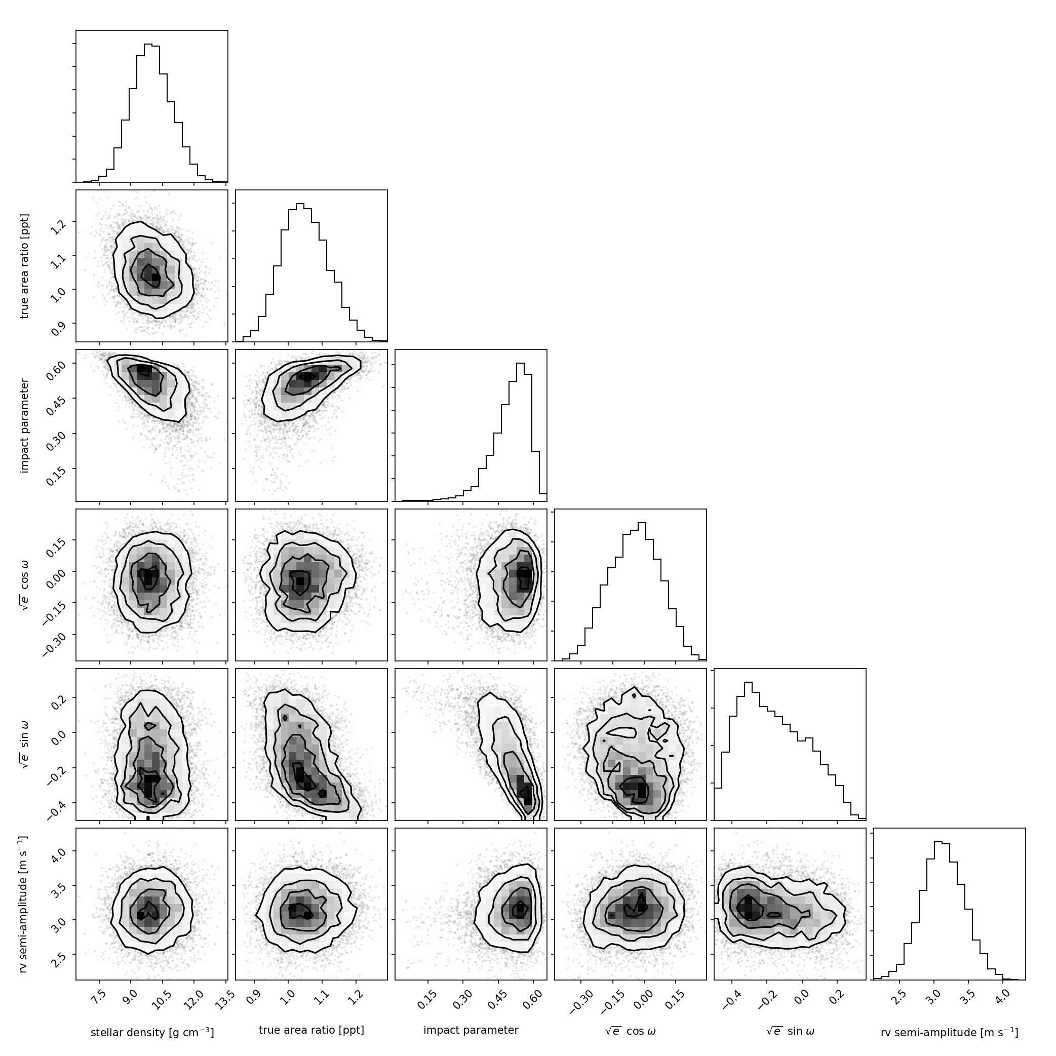
Figure 14: Marginal and joint parameter posterior densities for the sampling parameters describing LTT 3780 b.

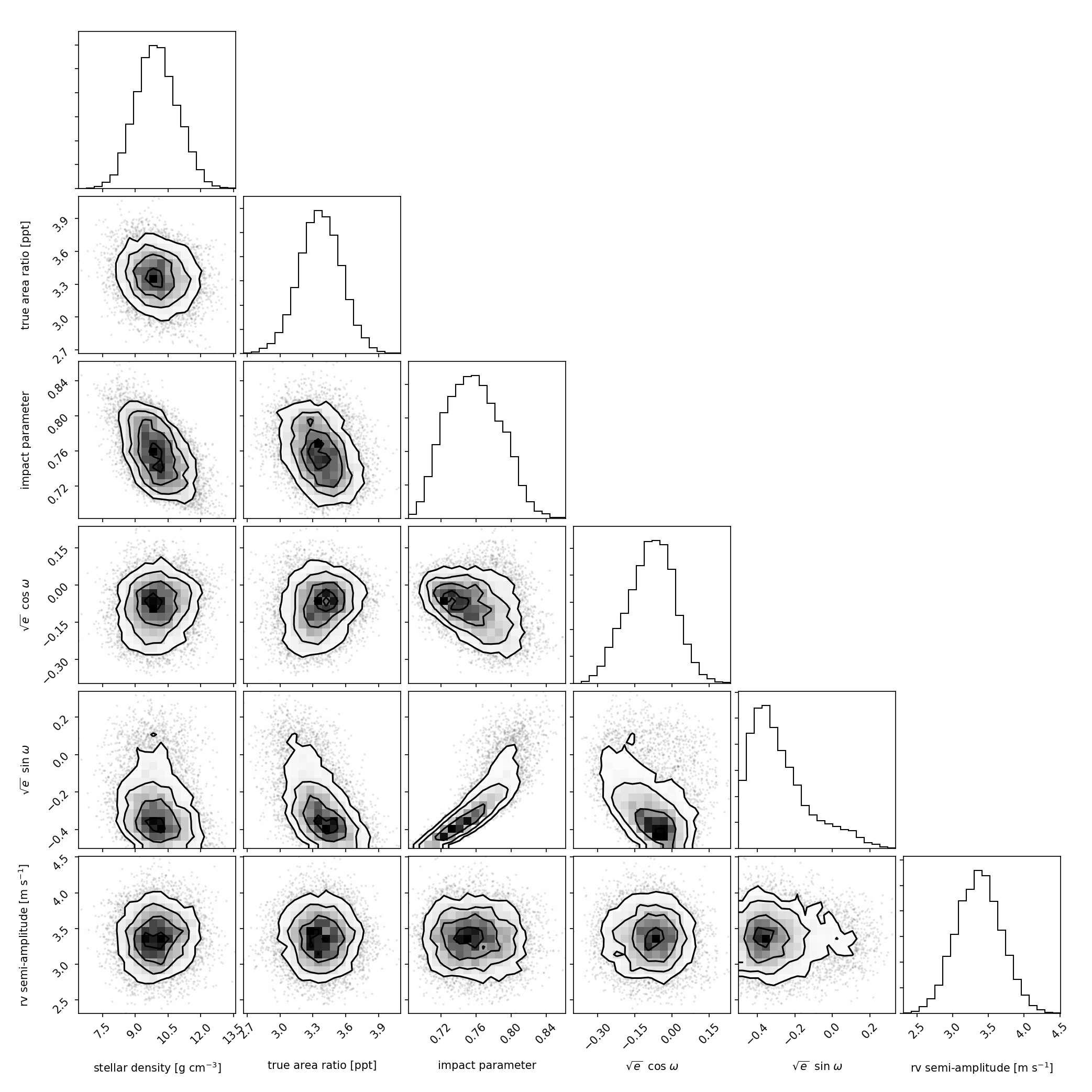
Figure 15: Marginal and joint parameter posterior densities for the sampling parameters describing LTT 3780 c.

Finally, we report the model posterior parameter estimates in Table 3. The posterior model is shown in Figs. 7 and 8, and parameter posteriors are shown for selected parameters in Figs. 14 and 15 in Appendix B.

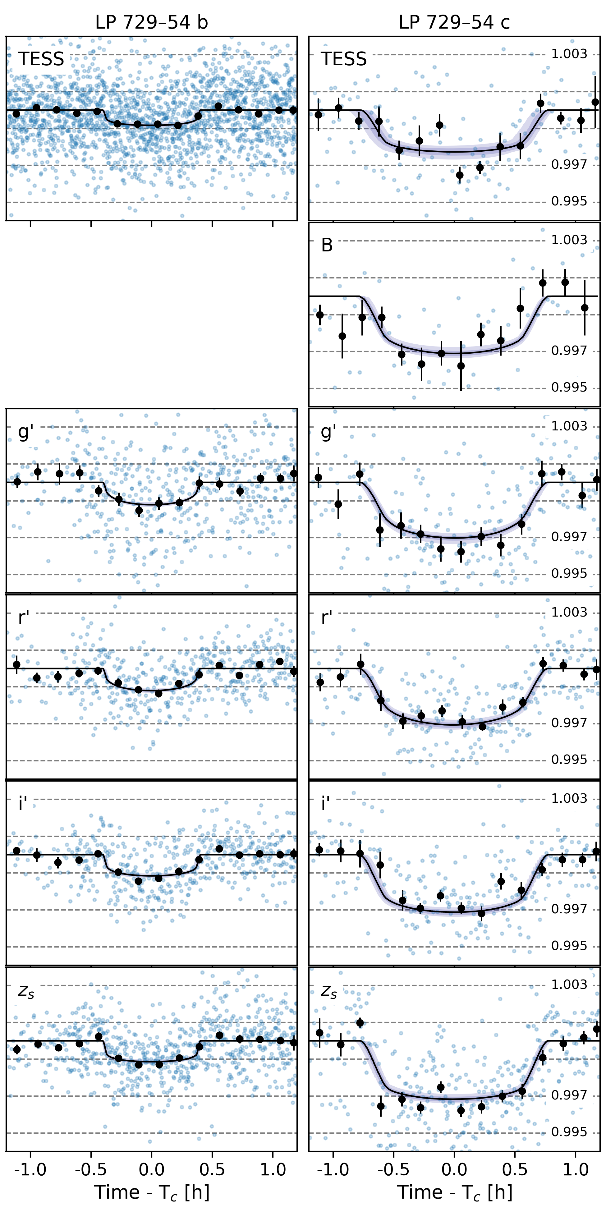
Figure 8: Combined and phase-folded transits of LTT 3780 b and c for each passband. The blue points show the original photometry with the median baseline model removed, the black dots with error bars show the photometry binned to 10 min resolution, the black line shows the median posterior model, and the dark and light shaded areas show the 68 % and 95 % model posterior percentile limits, respectively.

Table 3: Posterior estimates for the stellar and planetary parameters from the combined analysis.

Quantity	Notation	Unit	LTT 3780 b	LTT 3780 c
Orbit
Transit epoch	$T_{0}$	BJD	$2458543.91281^{+0.00048}_{-0.00052}$	$2458546.8492^{+0.0016}_{-0.0017}$
Orbital period	$P$	d	$0.768377^{+1.4e-06}_{-1.4e-06}$	$12.252131^{+7.2e-05}_{-6.4e-05}$
Eccentricity	$e$	…	$0.064^{+0.075}_{-0.046}$	$0.115^{+0.07}_{-0.065}$
Argument of periastron	$\omega$	deg	$251\pm 66$	$250\pm 36$
Transit duration	$T_{14}$	h	$0.818^{+0.044}_{-0.022}$	$1.79^{+0.21}_{-0.21}$
Relative properties
Radius ratio	$k=R_{p}/R_{\star}$	…	$0.0324^{+0.0011}_{-0.001}$	$0.0580^{+0.0016}_{-0.0016}$
Scaled semi-major axsi	$a_{\mathrm{s}}=a_{p}/R_{\star}$	…	$6.77^{+0.22}_{-0.21}$	$42.9^{+1.4}_{-1.3}$
Impact parameter	$b=(a/R_{\star})\cos i_{\rm p}$	…	$0.518^{+0.059}_{-0.089}$	$0.756^{+0.034}_{-0.031}$
Absolute properties
Planet radius	$R_{p}$	$\mathrm{R_{\oplus}}$	$1.35^{+0.06}_{-0.06}$	$2.42^{+0.10}_{-0.10}$
Planet mass	$M_{p}$	$\mathrm{M_{\oplus}}$	$2.34^{+0.24}_{-0.23}$	$6.29^{+0.63}_{-0.61}$
Mean density	$\rho_{p}$	$\mathrm{g\,cm^{-3}}$	$5.24^{+0.94}_{-0.81}$	$2.45^{+0.44}_{-0.37}$
Semi-major axis	$a_{p}$	au	$0.01203^{+0.00054}_{-0.00053}$	$0.0762^{+0.0034}_{-0.0034}$
Gravitational acceleration	$g_{p}$	$\mathrm{m\,s^{-2}}$	$12.6^{+1.8}_{-1.6}$	$10.5^{+1.5}_{-1.3}$
Equilibrium temperature	$T_{\mathrm{eq}}$	K	$1000^{+98}_{-100}$	$397^{+39}_{-40}$
Inclination	$i_{p}$	deg	$85.9^{+0.59}_{-0.50}$	$89.08^{+0.11}_{-0.13}$
Insolation	$S_{p}$	$S_{\oplus}$	$116^{+11}_{-10}$	$2.88^{+0.28}_{-0.25}$

6 Discussion

6.1 LTT 3780 b and c: two planets in the same system straddling the radius gap

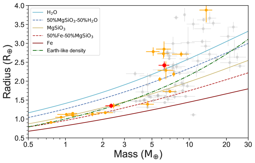
Figure 9: Mass-radius diagram for all planets with mass and radius measurement better than 20 % (from the TEPCat database of well-characterised planets; Southworth 2011). M-dwarf host planets are shown in orange, LTT 3780 b and LTT 3780 c with red dots. Theoretical models (Zeng et al., 2016) are overplotted using different lines and colours.

The LTT 3780 system consists of two small transiting planets. The ultra-short-period planet LTT 3780 b ($P_{\mathrm{b}}$ $\approx$ $0.77$ d) has a radius of $R_{\mathrm{b}}$ = $1.35^{+0.06}_{-0.06}$ $\mathrm{R_{\oplus}}$ and a mass of $M_{\mathrm{b}}$ = $2.34^{+0.24}_{-0.23}$ $\mathrm{M_{\oplus}}$, yielding a mean density of $\rho_{\mathrm{b}}$ = $5.24^{+0.94}_{-0.81}$ ${\rm g\,cm^{-3}}$. The outer planet LTT 3780 c ($P_{\mathrm{c}}$ $\approx$ $12.25$ d) has a radius of $R_{\mathrm{c}}$ = $2.42^{+0.10}_{-0.10}$ $\mathrm{R_{\oplus}}$ and a mass of $M_{\mathrm{c}}$ = $6.29^{+0.63}_{-0.61}$ $\mathrm{M_{\oplus}}$, yielding a mean density of $\rho_{\mathrm{c}}$ = $2.45^{+0.44}_{-0.37}$ ${\rm g\,cm^{-3}}$. This is the first planetary system around an M dwarf with two planets located on opposite sides of the radius gap (Fulton et al., 2017; Fulton & Petigura, 2018) that separates super-Earths from sub-Neptunes.

The positions of LTT 3780 b and LTT 3780 c on the mass-radius diagram are shown in Fig. 9 in comparison to the sample of small transiting planets ($R_{p}$ $\leq$ 4 $\mathrm{R_{\oplus}}$) whose masses and radii have been derived with a precision better than 20 % . The bulk densities of the two planets are significantly different, and their positions in the mass–radius diagram indicate substantially different compositions. Planet LTT 3780 b is compatible with an Earth-like bulk composition, ranging from 50 % silicate and 50 % iron to 100 % silicate. On the other hand, LTT 3780 c has a bulk density consistent with a volatile-dominated world.

The architecture of the LTT 3780 planetary system is consistent with those of other systems hosting two or more small, close-in planets located on opposite sides of the radius gap: Kepler-10 bc (Dumusque et al., 2014), K2-106 bc (Sinukoff et al., 2017; Guenther et al., 2017), HD 3167 bc (K2-96 bc; Christiansen et al., 2017; Gandolfi et al., 2017), GJ 9827 bcd (K2-135 bcd; Niraula et al., 2017; Prieto-Arranz et al., 2018), K2-138 bcdef (Christiansen et al., 2018; Lopez et al., 2019), HD 15337 bc (TOI-402 bc; Gandolfi et al., 2019; Dumusque et al., 2019), and K2-36 bc (Damasso et al., 2019). In all these systems, the close-in planets have smaller radii and higher mean densities, consistent with a rocky terrestrial composition, and the outer planets have larger radii and lower mean densities, suggesting that they are composed of rocky cores surrounded by light, hydrogen-dominated or water envelopes (see Fig. 10). This result agrees with current theoretical scenarios that explain the existence of the radius gap by atmospheric escape (Owen & Wu, 2017; Jin & Mordasini, 2018).

All previously-known stars with small planets located on opposite sides of the radius gap have warmer effective temperatures and higher masses than LTT 3780. Except for GJ 9827, host stars effective temperatures and masses range between 4920 K and 5810 K and 0.80 M_⊙ and 0.93 M_⊙, respectively. The previous smallest and coolest such star host, GJ 9827, has $T_{\rm eff}\approx$ 4260 K and $M\approx$ 0.66 M_⊙, consistent with its late K spectral type (Joy & Abt, 1974; Bidelman, 1985; Stephenson, 1986). However, LTT 3780 is significantly cooler ($T_{\rm eff}\approx$ 3360 K) and, correspondingly, less massive ($M\approx$ 0.38 M_⊙).

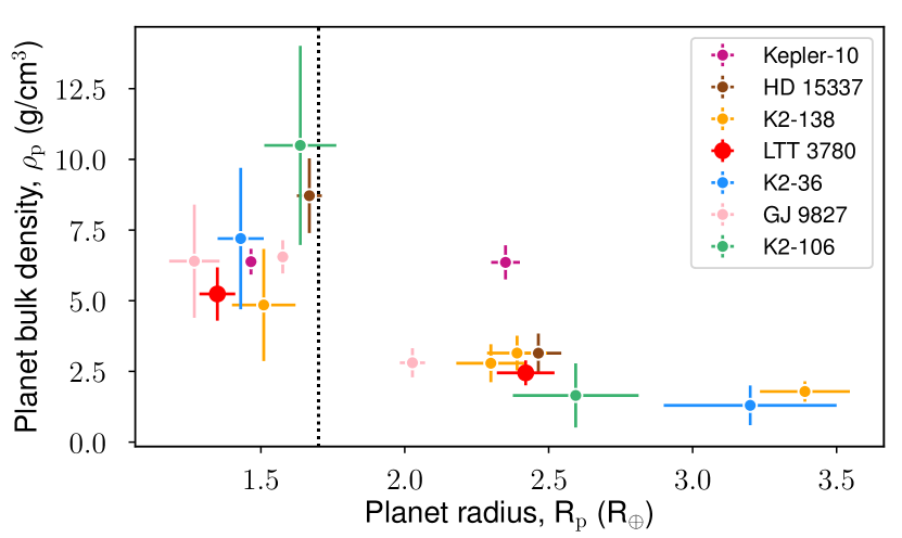
Figure 10: Radius–density diagram for multi-planet systems with planets on both sides of the radius gap. Different colours represent the different planetary systems, with the LTT 3780 planets marked and labelled in red. The vertical dotted line marks the centre of the radius gap at 1.7 $\mathrm{R_{\oplus}}$.

6.2 The ultra-short period planet LTT 3780 b

With orbital period of $P_{\mathrm{b}}$ $\approx$ $0.77$ d, LTT 3780 b belongs to the population of ultra-short period planets (USPs) and joins the relatively small group of transiting USPs with masses precisely measured via radial velocities and, hence, determined bulk densities. Taking into account the density of LTT 3780 b ($\rho_{\mathrm{b}}$ = $5.24^{+0.94}_{-0.81}$ ${\rm g\,cm^{-3}}$), this USP has probably undergone significant evolution and lost its primary, hydrogen-dominated atmosphere. The low luminosity of LTT 3780, as expected from its late spectral type, is counterbalanced by the short semi-mayor axis of LTT 3780 b, which leads to a strong planetary insolation ($S_{\mathrm{b}}$= $116^{+11}_{-10}$ $S_{\oplus}$).

The stellar properties of LTT 3780 and GJ 1151 (M4.5 V) are very similar (Passegger et al., 2018), both being relatively quiet stars. Although LTT 3780 is more distant from Earth and about half a magnitude fainter, it is worth searching for low-frequency radio emission from LTT 3780 possibly generated by the interaction of the star’s magnetospheric plasma with its USP, as suggested in the case of GJ 1151 (Vedantham et al., 2020).

6.3 System architecture

The architecture of the LTT 3780 system is analogous to that of Kepler-10, which has a (slightly larger and commensurately more massive) rocky planet with an orbital period about 10 % longer than that of LTT 3780 b (Batalha et al., 2011), and an outer planet with orbital period of 45 d, whose radius is within a few percent of that of LTT 3780 c (the mass of Kepler-10 c is poorly-constrained; Fressin et al., 2011; Weiss et al., 2016), and whose orbit is also inclined by $\sim$5–6 deg with respect to its inner ultra-short-period sibling. Multi-transiting planetary systems have few planets with orbital periods less than 1.6 d (Lissauer et al., 2014), and the high inclination of these two well-studied multi-planet systems with USPs (the inclinations of most other USP in Kepler multi-planet systems are not well constrained) supports the hypothesis that this paucity results at least in part from typical USPs being more highly inclined with respect to their planetary companions than the 1–2 deg value typical for Kepler multi-planet systems found by Fabrycky et al. (2014).

6.4 Atmospheric scenarios for LTT 3780 c

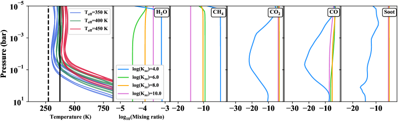
Figure 11: Left panel: Simulated temperature structures of LTT 3780 c assuming a substantial primary atmosphere. Blue, green, and red curves represent the temperature profiles at different effective temperatures of 350, 400, and 450 K, respectively. Different profiles within each group are caused by different atmospheric metallicity and C/O ratio. There are 27 temperature structures in total. The dashed and solid black vertical lines mark 273.15 K (0°C) and 373.15 K (100°C) for reference. Remaining panels: Examples of atmospheric abundances of H2O, CH4, CO2, CO, and soot (haze particles), for solar metallicity and C/O ratio, and effective temperature of 400 K, resulting from the photo-chemical simulations at different vertical mixing strengths.

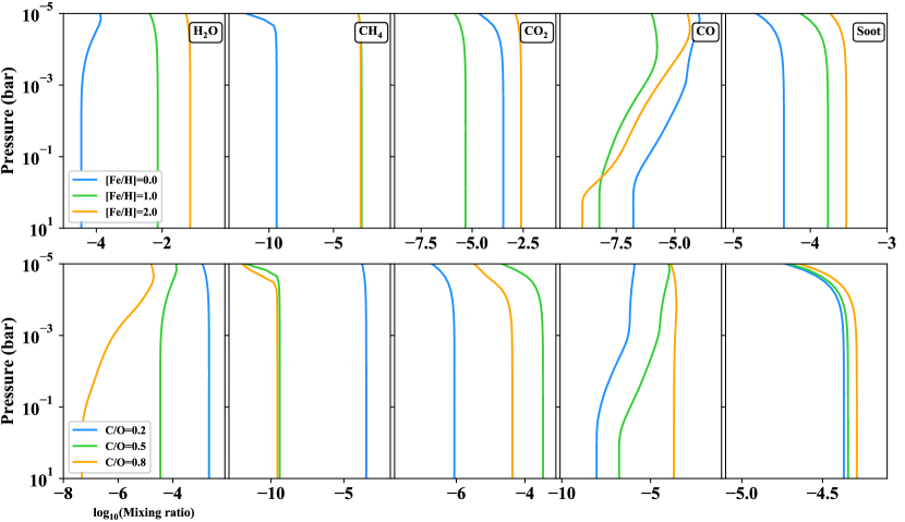
Figure 12: Abundances of several atmospheric constituents at $T_{\rm eff}=400$ K. Top panels: Solar C/O ratio, and K_zz=10⁶ cm² s^-1. Bottom panels: Solar metallicity and C/O ratios varying from 0.2 to 0.8.

The estimated radii of LTT 3780 b and c provide a unique opportunity to study the mechanisms that shape the Fulton gap (Fulton et al., 2017). While the proximity of LTT 3780 b to its host star and its relatively small radius suggest the challenging nature of maintaining an atmosphere on this planet, characterisation of the atmosphere of LTT 3780 c will shed light on the nature of the dominant atmospheric processes in action on this planet. While LTT 3780 c is not as appealing a target as TRAPPIST planets (TSM $\in$ 20–45; Gillon et al., 2017; Grimm et al., 2018) or LHS 1140 b (TSM$\sim$65; Dittmann et al., 2017), its transmission spectroscopy metric ($\mathrm{TSM}$) defined by Kempton et al. (2018) for JWST/NIRISS is $\sim$ 122, which is above the cutoff of TSM = 90 suggested for atmospheric characterisation of planets with radii 1.5 ¡ $R_{p}$ ¡ 2.75 $\mathrm{R_{\oplus}}$ with JWST/NIRISS.

In order to explore possible atmospheric scenarios of LTT 3780 c, we followed the approach outlined in Molaverdikhani et al. (2019a), assuming that the planet sustains a substantial primary atmosphere. First we modelled the atmosphere self-consistently over a wide range of parameters using petitCODE (Mollière et al., 2015, 2017). Given the uncertainties on the estimated equilibrium temperature of LTT 3780 c and possible missing feedback mechanisms in our self-consistent simulations, we chose the effective temperature as a free parameter with values of 350, 400, and 450 K (the equilibrium temperature derived for LTT 3780 c is $397^{+39}_{-40}$ K). Since the interior heat budget of exoplanets is not well understood, we assumed an interior heat budget contribution similar to that of Earth, i.e. $\sim$0.027 (e.g. Archer, 2011). Slight deviations of the interior heat budget from this value do not change the results significantly. The atmospheric metallicity of planets seems to increase for less massive planets, both in the Solar System (e.g. Molaverdikhani et al., 2019b) and beyond (Wakeford et al., 2017). Thus, we assumed three different metallicities, namely 1$\times$, 10$\times$, and 100$\times$ solar metallicity, similar to those used by Luque et al. (2019). In addition, we also investigated the role of the carbon-to-oxygen ratio (C/O) in the atmosphere of LTT 3780 c, assuming C/O = 0.2 (sub-solar), 0.5 ($\sim$solar), and 0.8 (super-solar). Altogether, 27 self-consistent temperature structures were calculated (Fig. 11). No Earth-like cloud formation was included in our models.

In the next step we used these temperature structures as the input of our photochemical model (ChemKM; Molaverdikhani et al., 2019a, 2020) to estimate abundances of atmospheric constituents. Studying the atmosphere of this planet required a validated chemical network over the assumed equilibrium temperatures. We therefore used the Hébrard et al. (2012) full kinetic network (including 788 reactions and 135 H-C-O-N bearing species) and an updated version of their ultraviolet absorption cross-sections and branching yields. While the formation of hydrocarbon-based hazes is not fully understood (e.g. Hörst et al., 2018), it is believed that these processes start with the photolysis of haze precursor molecules such as CH4, C2H2, HCN, and C6H6 (e.g. Molaverdikhani et al., 2020). The chosen chemical network included all these precursor molecules and represented the haze particles collectively as one constituent called ‘soot’ (e.g. Lavvas & Koskinen, 2017). This soot included C8H6, C8H7, C10H3, C12H3, C12H10, C14H3, C2H4N, C2H3N2, C3H6N, C4H3N2, C4H8N, C5HN, C5H3N, C5H4N, C5H6N, C9H6N, C3H3O, C3H5O, C3H7O, and C4H6O, following the convention outlined by Hébrard et al. (2012).

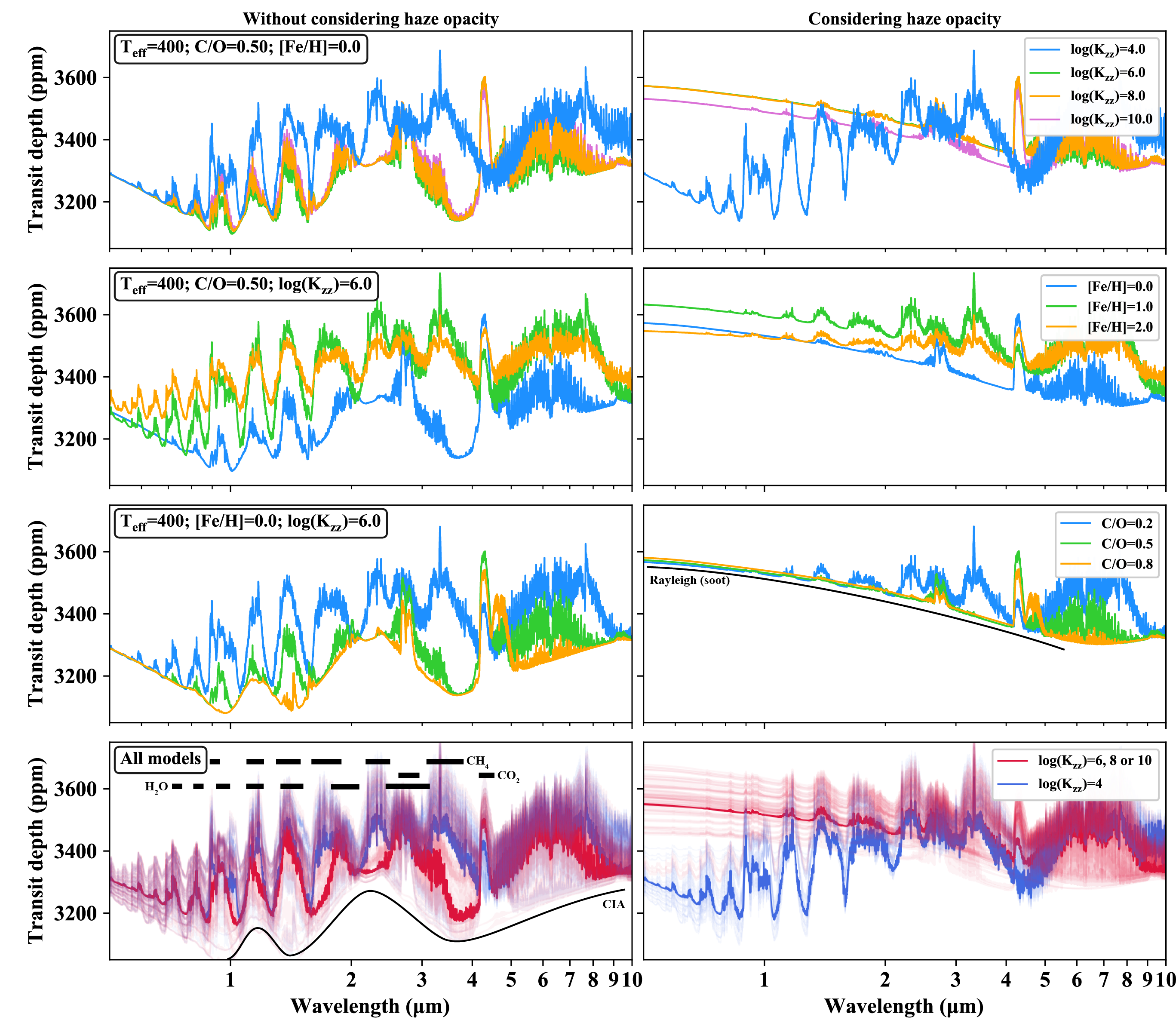
Figure 13: Synthetic transmission spectra of LTT 3780 c. Left panels: Transmission spectra calculated without taking into account the opacity contribution of haze particles (soot). The top-left panel shows the variation of spectra with the strength of vertical mixing, corresponding to the cases in Fig. 11. The two middle panels also correspond to the two cases in Fig. 12. The bottom-left panel represents the transmission spectra of all 108 models in the two categories of strong (10⁶, 10⁸, or 10¹⁰ cm²s^-1) and weak (10⁴ cm²s^-1) vertical mixing. Right panels: Same as left panels, but with opacity of haze particles taken into account.

The temperature of GJ 667C, another M-dwarf exoplanet host, is estimated to be around 3330 K (Neves et al., 2014), similar to that of LTT 3780. Consequently, we estimated the flux of LTT 3780 in the range of X-ray to optical wavelengths using GJ 667C data, obtained from the MUSCLES database (France et al., 2016). In addition to photolysis, we considered the effect of vertical mixing in the photochemical simulations by considering four values, 10⁴, 10⁶, 10⁸, and 10¹⁰ $\mathrm{cm\,s^{-2}}$, covering a wide range of possibilities from terrestrial values to tidally locked gaseous planets. In total, 108 photochemical models were calculated.

Examples of H2O, CH4, CO2, CO, and soot (haze particles) abundances are shown in Fig. 11, assuming an effective temperature of 400 K, solar metallicity and solar C/O. In general, chemical depletion of H2O and CH4 are noticeable at strong vertical mixing conditions, i.e. 10⁶, 10⁸ and 10¹⁰ $\mathrm{cm\,s^{-2}}$, while CO2, CO, and soot particles show an enhancement in abundance under such conditions. Figure 12 isolates the effect of metallicity (upper panels) and C/O ratio (lower panels) on the abundance of H2O, CH4, CO2, CO, and soot. For these illustrated examples, we assumed an effective temperature of 400 K and a vertical mixing strength (K_zz) of 10⁶ cm² s^-1. In general, increasing the metallicity would enhance the production of most species at most altitudes under these conditions. However, given the highly non-linear nature of atmospheric feedback, some species could behave differently; see e.g. CO in the upper panel of Fig. 12. The C/O ratio is modified by changing the oxygen elemental abundance and keeping the carbon elemental abundance the same. This represents a scenario in which gas or planetesimals accrete onto a forming planet with different water content, while the carbon content assumed to remain the same. Hence, variations of the C/O should not change methane abundances very much, as it has no oxygen compound. However, as a function of the dependency of the chemical formation pathway of a constituent on the formation of oxygen-bearing species, as well as their radiative feedback, the abundance of hydrocarbons could change with the C/O ratio. The lower panels of Fig. 12 illustrate such an example, where CH4 remains mostly insensitive to the C/O ratio at C/O $\geq$ 0.5, but a C/O of 0.2 results in an enhanced abundance of methane. This unexpected methane production (or lack of methane depletion) is largely caused by how disequilibrium processes, namely photo-dissociation and atmospheric mixing, act on this planet. In addition, a variation of the C/O ratio affects the H2O abundance significantly, as is shown in the lower-left panel of Fig. 12.

We find that, due to the relatively low temperature of LTT 3780 c, any vertical mixing stronger than 10⁴ cm² s^-1 could strongly quench the abundance of most species. This appears as a nearly constant abundance profile for any given species at such K_zz. Figure 11 illustrates examples for this at three different values of K_zz. This is particularly important for haze particles because under these circumstances their abundance becomes very significant at all altitudes and can therefore affect the spectra by obscuring the atomic and molecular features in the optical and NIR ranges.

Figure 13 shows synthetic transmission spectra of the above-mentioned cases calculated using petitRADTRANS (Mollière et al., 2019). We considered two cases, one without haze opacity, and the other with haze opacity assuming a mono-disperse particle size distribution with an effective particle radius of 50 nm (e.g. Tomasko et al., 2005; Trainer et al., 2006). The change in the C/O ratio had only a small effect compared to other parameters, where it mainly affected the spectral significance of H2O. On the other hand, a combination of low metallicity and strong vertical mixing could change the transmission spectra significantly. Under such conditions, the atmosphere becomes methane-depleted. The case of methane-depletion at K_zz $>$ 10⁴ cm²s^-1 and [Fe/H] = 0.0 (solar metallicity) is shown in the top panels of Fig. 13. Similarly, at K_zz = 10⁶ cm² s^-1, solar metallicity results in the depletion of methane, second row from top in Fig. 13. Another key feature is the presence of CO2 at around 4.3 $\mathrm{\mu m}$ with a spectral difference above 200 ppm for most cases with strong mixing. Prominent spectral features (associated with CH4, H2O, and CO2) are marked in the lower left panel of Fig. 13. The collision-induced absorption (CIA) continuum is also shown in the same panel.

The right panels of Fig. 13 show the same cases as the left panels, except that they include the opacity of haze particles in the synthetic transmission spectra of LTT 3780 c. The significance of this opacity in the spectra is evident. As mentioned, haze production is mainly associated with strong vertical mixing; see top right and bottom right panels. Including the haze opacity makes the detection of methane-depleted atmospheres more challenging. However, the CO2 feature at 4.3 $\mathrm{\mu m}$ remains a distinct and key feature for the detection of atmospheric features in LTT 3780 c in the NIR. Our simulations suggest that JWST instruments would be able to detect the CO2 spectral feature, as their noise floor is much lower than the spectral significance of this feature (Greene et al., 2016).

In summary, despite many degeneracies between the synthetic spectra, looking for the presence of H2O, CH4, CO2, and haze particles (Rayleigh scattering) with future facilities such as JWSTcould hint at the type and significance of the dominant atmospheric processes on LTT 3780 c.

On a final note, the extension of simulations to 3D models is likely to favour more pronounced cloud formation and stronger disequilibrium processes on the night side and their extension to at least the morning limb (e.g. Molaverdikhani et al., 2020). Hence, 3D simulations are needed to evaluate the significance of these processes. Moreover, further analyses are needed to study the processes by which the primary atmosphere of both LTT 3780 b and c could be removed, and a secondary atmosphere could be formed and maintained.

6.5 An independent analysis of the LTT 3780 system by HARPS and HARPS-N

Following the announcement of the planet candidates TOI–732.01 and 02 in 2019 May, multiple precision RV instrument teams began working toward the mass characterisation of these potential planets. The present study presents the subset of those efforts from CARMENES, but we are aware that the joint HARPS and HARPS-N team has also submitted a paper presenting their own RV time series and analysis (Cloutier et al., 2020). Although the submissions of these complementary studies were coordinated between the two groups, their respective data, analyses, and write-ups were intentionally conducted independently.

7 Conclusions

We report here the discovery and detailed characterisation of a planetary system around the bright M dwarf LTT 3780, composed of two small transiting planets straddling the radius gap. Transit signals of both planets are detected in the TESS photometry and confirmed by ground-based facilities. These ground-based photometric observations of LTT 3780 allow us to confirm the planetary nature of the candidates and determine the true radii of planets thanks to aperture photometry uncontaminated by close-in stars. Prompt RV follow-up with the CARMENES spectrograph provides a precise mass determination of both planets.

LTT 3780 b is a very hot ($T_{\mathrm{eq}}$ = $1000^{+98}_{-100}$ K), ultra-short period ($P_{\mathrm{b}}$ $\approx$ $0.77$ d) planet that is slightly larger in size than the Earth ($R_{\mathrm{b}}$ = $1.35^{+0.06}_{-0.06}$ $\mathrm{R_{\oplus}}$) but has an equal bulk density. With radius $R_{\mathrm{c}}$ = $2.42^{+0.10}_{-0.10}$ $\mathrm{R_{\oplus}}$, LTT 3780 c is located on the opposite side of the radius gap, exactly at the peak of the sub-Neptune distribution that is believed to be a population of gas-dominated planets. With an equilibrium temperature of $T_{\mathrm{eq}}$ = $397^{+39}_{-40}$ K, LTT 3780 c is an excellent target for atmospheric characterisation with the upcoming JWST.

Appendix A Long tables

Table 4: Radial velocities of LTT 3780.

BJDTDB-2 450 000	RV ($\mathrm{m\,s^{-1}}$)	$\sigma_{\mathrm{RV}}$ ($\mathrm{m\,s^{-1}}$)
3.5 m Calar Alto/CARMENES-VIS
8844.63067	3.676	5.861
8844.75146	-7.469	3.631
8846.60074	-1.753	1.615
8846.71780	-2.432	1.258
8848.62456	5.964	1.383
8848.73609	8.577	1.335
8849.59266	5.041	1.453
8849.73669	1.953	1.648
8850.61843	1.189	1.191
8850.72764	-1.199	1.331
8851.63152	0.324	1.133
8851.74504	3.429	1.170
8852.65899	5.364	1.325
8852.75676	-0.902	1.097
8854.61164	-8.242	1.798
8855.60409	0.717	1.543
8855.74490	-2.347	1.574
8856.58282	-2.463	1.401
8856.72077	-8.844	1.582
8857.57560	-7.257	1.523
8858.63243	1.425	2.106
8860.55597	6.827	2.478
8860.67971	1.469	2.199
8864.56029	-4.091	1.859
8865.55825	6.382	2.696
8865.67852	3.557	1.896
8866.61374	2.104	2.638
8877.52010	0.316	1.954
8877.68512	-1.075	2.024
8878.57708	-1.038	1.918
8880.63111	-5.071	1.894
8880.71831	-2.735	2.399
8881.50534	-2.453	1.370
8881.65959	-0.782	1.341
8882.48468	-1.096	1.643
8882.67088	1.903	1.530
8883.52731	1.816	1.454
8883.68305	-2.280	1.520
8884.52841	-0.715	1.440
8884.67457	2.912	1.432
8885.51388	6.990	1.509
8885.63103	6.912	1.494
8887.54307	-3.888	3.347
8889.60111	0.741	1.967
8890.55909	-0.965	1.680
8891.50814	-6.148	1.589
8893.55000	-1.000	1.539
8894.51095	-8.253	1.487
8895.52663	-0.796	1.523
8896.50587	0.123	1.674
8897.47151	-1.596	1.627
8898.57582	-5.761	2.995
Subaru/IRD
8828.06968	1.950	2.460
8828.07559	1.240	2.460
8828.08218	4.990	2.460
8828.08811	-2.390	2.410
IRTF/iSHELL
8874.08622	-9.389	11.841
8875.02099	-4.854	9.743
8894.99312	4.020	10.855
8898.96755	-14.658	5.359
8899.95713	-17.587	8.026
8900.95157	-0.664	7.871
8907.99311	11.516	10.568
8911.02803	5.116	7.481

Appendix B Joint modelling

B.1 Model parameter priors

Table 5: Parameter priors for the combined modelling of transit light curves and RV observations.

Parameter name	Prior	Unit	Description
Parameters for planet b
$P_{b}$	$\mathcal{N}(0.768418,0.0002)$	d	Orbital period
$t_{0,b}$	$\mathcal{N}(2458543.9115,0.0036)$	d	Time of transit centre
$k^{2}_{b}$	$\mathcal{U}(0.0,0.01)$	…	True area ratio
$b_{b}$	$\mathcal{U}(0.0,1.0)$	…	Impact parameter
$K_{b}$	$\mathcal{U}(0.0,36.0)$	m s-1	Radial velocity semi-amplitude
$S_{1,b}=\sqrt{e_{b}}\sin\omega_{b}$	$\mathcal{U}(-0.5,0.5)$	…	Parametrisation for $e$ and $\omega$
$S_{2,b}=\sqrt{e_{b}}\cos\omega_{b}$	$\mathcal{U}(-0.5,0.5)$	…	Parametrisation for $e$ and $\omega$
Parameters for planet c
$P_{c}$	$\mathcal{N}(12.254218,0.006^{2})$	d	Orbital period
$t_{0,c}$	$\mathcal{N}(2458546.8484,0.0042^{2})$	d	Time of transit centre
$k^{2}_{c}$	$\mathcal{U}(0.0,0.01)$	…	True area ratio
$b_{c}$	$\mathcal{U}(0.0,1.0)$	…	Impact parameter
$K_{c}$	$\mathcal{U}(0.0,36.0)$	m s-1	Radial velocity semi-amplitude
$S_{1,c}=\sqrt{e_{c}}\sin\omega_{c}$	$\mathcal{U}(-0.5,0.5)$	…	Parametrisation for $e$ and $\omega$
$S_{2,c}=\sqrt{e_{c}}\cos\omega_{c}$	$\mathcal{U}(-0.5,0.5)$	…	Parametrisation for $e$ and $\omega$
Flux contamination parameters
$c_{{TESS}}$	$\mathcal{U}(0.0,0.99)$	…	TESS contamination
$c_{\textnormal{gb}}$	$\mathcal{U}(0.0,0.99)$	…	Ground-based contamination in $r^{\prime}$
$T_{\mathrm{eff},h}$	$\mathcal{N}(3360.0,51)$	K	Host star $T_{\mathrm{eff}}$
$T_{\mathrm{eff},c}$	$\mathcal{U}(2500,12000)$	K	Contaminant $T_{\mathrm{eff}}$
Stellar parameters
$\rho_{*}$	$\mathcal{N}(9.6,1.0)$	g cm-3	Stellar density
$q_{1,f}$	LDTk	…	Limb-darkening q1 for passband $f$
$q_{2,f}$	LDTk	…	Limb-darkening q2 for passband $f$
Additional parameters
$\log e_{i}$	$\mathcal{U}(-4,0)$	-	$\log 10$ average white noise for light curve $i$
$z_{i}$	$\mathcal{N}$	…	Baseline constant (intercept) for light curve $i$
$c_{i,j}$	$\mathcal{N}$	…	Baseline coefficient for light curve $i$ covariate $j$
RV instrumental parameters
$\gamma_{\textnormal{CARMENES}}$	$\mathcal{U}(-100,100)$	m s-1	Systemic velocity for CARMENES
$\gamma_{\textnormal{IRD}}$	$\mathcal{U}(-100,100)$	m s-1	Systemic velocity for Subaru/IRD
$\gamma_{\textnormal{iSHELL}}$	$\mathcal{U}(-100,100)$	m s-1	Systemic velocity for IRTF/iSHELL

B.2 Posterior distribution functions