A pair of TESS planets spanning the radius valley around the nearby mid-M dwarf LTT 3780

Abstract

We present the confirmation of two new planets transiting the nearby mid-M dwarf LTT 3780 (TIC 36724087, TOI-732, $V=13.07$, $K_{s}=8.204$, $R_{s}$=0.374 R_⊙, $M_{s}$=0.401 M_⊙, d=22 pc). The two planet candidates are identified in a single TESS sector and are validated with reconnaissance spectroscopy, ground-based photometric follow-up, and high-resolution imaging. With measured orbital periods of $P_{b}=0.77$ days, $P_{c}=12.25$ days and sizes $r_{p,b}=1.33\pm 0.07$ R_⊕, $r_{p,c}=2.30\pm 0.16$ R_⊕, the two planets span the radius valley in period-radius space around low mass stars thus making the system a laboratory to test competing theories of the emergence of the radius valley in that stellar mass regime. By combining 63 precise radial-velocity measurements from HARPS and HARPS-N, we measure planet masses of $m_{p,b}=2.62^{+0.48}_{-0.46}$ M_⊕ and $m_{p,c}=8.6^{+1.6}_{-1.3}$ M_⊕, which indicates that LTT 3780b has a bulk composition consistent with being Earth-like, while LTT 3780c likely hosts an extended H/He envelope. We show that the recovered planetary masses are consistent with predictions from both photoevaporation and from core-powered mass loss models. The brightness and small size of LTT 3780, along with the measured planetary parameters, render LTT 3780b and c as accessible targets for atmospheric characterization of planets within the same planetary system and spanning the radius valley.

1 Introduction

Since the commencement of its prime mission in July 2018, NASA’s Transiting Exoplanet Survey Satellite (TESS; Ricker et al. 2015) has unveiled many of the closest transiting exoplanetary systems to our solar system. The proximity of many of these systems make their planets ideal targets for the detailed characterization of their bulk compositions and atmospheric properties. Systems of multiple transiting planets are of particular interest as they afford the unique opportunity for direct comparative planetology, having formed within the same protoplanetary disk and evolved around the same host star.

The occurrence rate of close-in planets features a dearth of planets between $1.7-2.0$ R_⊕ around Sun-like stars and between $1.5-1.7$ around low mass stars (Fulton et al., 2017; Mayo et al., 2018; Cloutier & Menou, 2020; Hardegree-Ullman et al., 2020). The so-called radius valley is likely a result of the existence of an orbital separation-dependent transition between primarily rocky planets and non-rocky planets that host extended H/He envelopes. A number of physical processes have been proposed to explain the existence of this rocky/non-rocky transition, including photoevaporation, wherein XUV heating from the host star drives thermal atmospheric escape preferentially on smaller, low surface gravity planets during the first 100 Myrs (Owen & Wu, 2013; Jin et al., 2014; Lopez & Fortney, 2014; Chen & Rogers, 2016; Owen & Wu, 2017; Jin & Mordasini, 2018; Lopez & Rice, 2018; Wu, 2019). Alternatively, the core-powered mass loss mechanism, wherein the dissipation of the planetary core’s primordial energy from formation drives atmospheric mass loss over Gyr timescales (Ginzburg et al., 2018; Gupta & Schlichting, 2019, 2020). Rather than resulting from the dissipation of primordial planetary atmospheres, the radius valley may instead arise from the superposition of rocky and non-rocky planet populations, with the former forming in a gas-poor environment after the dissipation of the gaseous protoplanetary disk (Lee et al., 2014; Lee & Chiang, 2016; Lopez & Rice, 2018).

Each of the aforementioned mechanisms make explicit predictions for the location of the rocky/non-rocky transition in the orbital period-radius space. Measurements of planetary bulk compositions in systems of multiple planets that span the radius valley therefore offer an opportunities to resolve the precise location of the rocky/non-rocky transition (Owen & Campos Estrada, 2020) and distinguish between the model predictions. Precise planetary bulk composition measurements for systems around a range of host stellar masses will enable the dependence of the radius valley on stellar mass to be resolved and consequently used to test competing models of the emergence of the radius valley (Cloutier & Menou, 2020, hereafter CM20).

Here we present the discovery and confirmation of the two-planet system around the nearby (d=22 pc) mid-M dwarf LTT 3780 from the TESS mission. The planets LTT 3780b and c span the rocky/non-rocky transition such that the characterization of their bulk compositions can be used to constrain emergence models of the radius valley by marginalizing over unknown system parameters such as the star’s XUV luminosity history. The brightness of LTT 3780 ($K_{s}=8.204$) and the architecture of its planetary system also make it an attractive target for the atmospheric characterization of multiple planets within the same planetary system. In Sect. 2 we present the properties of LTT 3780. In Sect. 3 we present the TESS light curve along with our suite of follow-up observations, including reconnaissance spectroscopy, ground-based photometry, high-resolution imaging, and precise radial-velocity measurements. In Sect. 4 we present our two independent analyses of our data, to ensure the robustness of our results, before concluding with a discussion and summary of our results in Sects. 5 and 6.

2 Stellar Characterization

LTT 3780 (LP 729-54, TIC 36724087, TOI-732) is a mid-M dwarf at a distance of 22 pc (Gaia Collaboration et al., 2018; Lindegren et al., 2018). Astrometry, photometry, and the LTT 3780 stellar parameters are reported in Table 1. The stellar $T_{\text{eff}}$ $=3331\pm 157$ K is taken from the TESS Input Catalog (TIC v8; Stassun et al., 2019) and is consistent with the value derived from the Stefan-Boltzmann equation ($3343\pm 150$ K). The stellar metallicity is weakly constrained by its SED and MIST isochrones (Dotter, 2016). The LTT 3780 mass and radius are derived from the stellar parallax and $K_{s}$-band magnitude, used to compute the absolute $K_{s}$-band magnitude $M_{K_{s}}$, and the empirically-derived M dwarf mass-luminosity and radius-luminosity relations from Benedict et al. (2016) and Mann et al. (2015) respectively. LTT 3780’s surface gravity is computed from its mass and radius. No photometric rotation period is apparent in either the TESS or ground-based photometry. However, the low value of $\log{R_{\text{HK}}^{\prime}}=-5.59$ is indicative of a chromospherically inactive star with likely a long rotation period (estimated $P_{\text{rot}}$ $=104\pm 15$ days; Astudillo-Defru et al., 2017).

Table 1: LTT 3780 stellar parameters.

Parameter	Value	Refs
LTT 3780, LP 729-54, TIC 36724087, TOI-732
Astrometry
Right ascension (J2000.0), $\alpha$	10:18:34.78	1,2
Declination (J2000.0), $\delta$	-11:43:04.08	1,2
RA proper motion, $\mu_{\alpha}$ [mas yr-1]	$-341.41\pm 0.11$	1,2
Dec proper motion, $\mu_{\delta}$ [mas yr-1]	$-247.87\pm 0.11$	1,2
Parallax, $\varpi$ [mas]	$45.493\pm 0.083$	1,2
Distance, $d$ [pc]	$21.981\pm 0.040$	1,2
Photometry
$V$	$13.07\pm 0.015$	3
$G_{\text{BP}}$	$13.352\pm 0.004$	1,4
$G$	$11.8465\pm 0.0005$	1,4
$G_{\text{RP}}$	$10.658\pm 0.002$	1,4
$T$	$10.585\pm 0.007$	5
$J$	$9.007\pm 0.030$	6
$H$	$8.439\pm 0.065$	6
$K_{s}$	$8.204\pm 0.021$	6
$W_{1}$	$8.037\pm 0.022$	7
$W_{2}$	$7.880\pm 0.019$	7
$W_{3}$	$7.771\pm 0.019$	7
$W_{4}$	$7.577\pm 0.166$	7
Stellar parameters
Spectral type	M4V	8
$M_{V}$	$11.36\pm 0.02$	9
$M_{K_{s}}$	$6.49\pm 0.02$	9
Effective temperature, $T_{\text{eff}}$ [K]	$3331\pm 157$	5
Surface gravity, $\log{g}$ [dex]	$4.896\pm 0.029$	9
Metallicity, [Fe/H] [dex]	$0.28^{+0.11}_{-0.13}$	9
Stellar radius, $R_{s}$ [R⊙]	$0.374\pm 0.011$	9
Stellar mass, $M_{s}$ [M⊙]	$0.401\pm 0.012$	9
Projected rotation velocity,
	$<1.3$	9
$v\sin{i}$ [km s-1]
$\log{R_{\text{HK}}^{\prime}}$	$-5.59\pm 0.09$	9
Estimated rotation period,
	$104\pm 15$	9
$P_{\text{rot}}$ [days]

Note. — References: 1) Gaia Collaboration et al. 2018 2) Lindegren et al. 2018 3) Reid et al. 2002 4) Evans et al. 2018 5) Stassun et al. 2019 6) Cutri et al. 2003 7) Cutri & et al. 2014 8) Scholz et al. 2005 9) this work.

LTT 3780 is the primary component of a visual binary system with an angular separation of $16.1^{\prime\prime}$ from the Gaia DR2 positions (Gaia Collaboration et al., 2018; Lindegren et al., 2018). The binary was previously identified to be co-moving from measures of each stellar component’s proper motion and spectroscopic distance (Luyten, 1979; Scholz et al., 2005). The common parallaxes and proper motions of LTT 3780 (alias LP 729-54) and its stellar companion LP 729-55 (TIC 36724086) were verified in Gaia DR2. Their angular separation of $16.1^{\prime\prime}$ implies a projected physical separation of 354 AU. The fainter companion star has $K_{s}=10.223\pm 0.021$ (i.e. $\Delta K_{s}=2.019$ mag) which corresponds to a mass and radius of $0.136\pm 0.004$ M_⊙ and $0.173\pm 0.005$ R_⊙. Given the stellar mass ratio of $q=0.340\pm 0.014$, the orbital period of the stellar binary at their projected physical separation is about 9100 years. Assuming a circular orbit, this corresponds to a negligible maximum radial velocity (RV) variation of $\lesssim 15$ cm s^-1 over the timescale of our RV observations presented in Sect. 3.5. We also calculated the secular acceleration of the binary system given its large proper motion (Table 1) to be $<10$ cm s^-1 year^-1. This RV variation is also well below the noise limit of our observations over our RV baseline.

The LTT 3780 planetary system may be an interesting test case of planet formation models in a binary systems. Although, the large physical separation of the stellar components likely resulted in isolated planet formation around LTT 3780.

3 Observations

3.1 TESS photometry

LTT 3780 was observed in TESS sector nine (i.e. orbits 25 and 26) for 27.26 days from UT February 28 to March 26, 2019 with CCD 1 on Camera 1. As a member of the Cool Dwarf target list (Muirhead et al., 2018), LTT 3780 was included in the TIC and in the Candidate Target List (CTL; Stassun et al., 2017) such that its light curve was sampled at 2-minute cadence. These data were processed by the NASA Ames Science Processing Operations Center (SPOC; Jenkins et al., 2016). The resulting Presearch Data Conditioning Simple Aperture Photometry (PDCSAP; Smith et al., 2012; Stumpe et al., 2012, 2014) light curve of LTT 3780 was corrected for dilution by known contaminating sources within the photometric aperture with a dilution factor of 0.713. According to the sector nine data release notes, the level of scattered light from the Earth in Camera 1 CCD 1 at the start of each orbit was high and resulted in no photometry or centroid positions being calculated during the first 1.22 days of orbit 25 nor in the first 1.12 days of orbit 26. Data collection was also paused for 1.18 days for data downloading close to the spacecraft’s time of perigee passage. Overall, a total of 24.08 days of science data collection was performed in TESS sector nine.

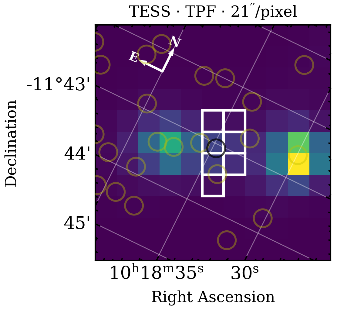
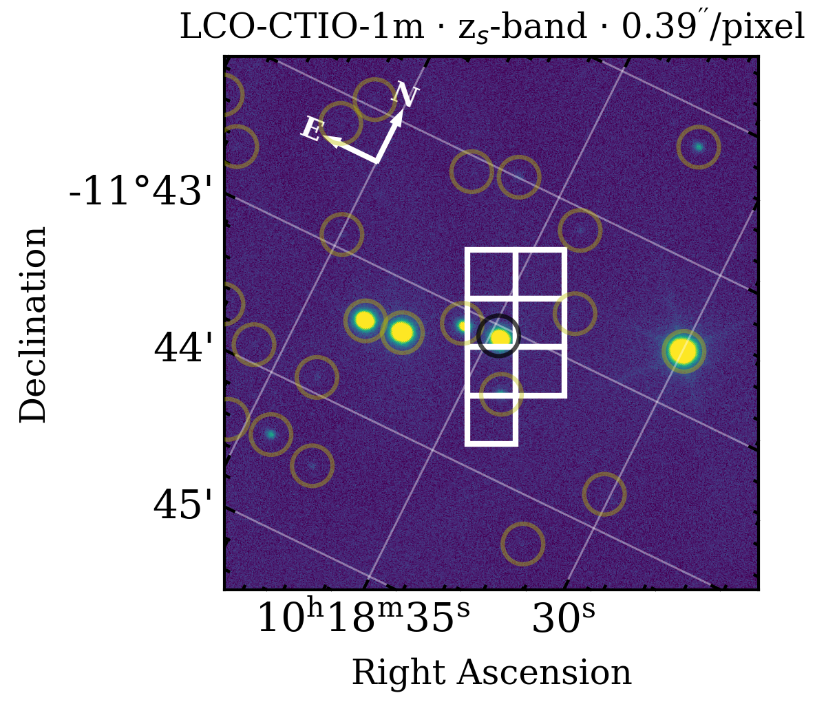
A sample image of the field surrounding LTT 3780 from the TESS target pixel files is shown in Figure 1. The TESS photometric aperture used to produce the PDCSAP light curve was selected to maximize photometric signal-to-noise (Bryson et al., 2010) and is overlaid in Figure 1. Blending in the TESS photometry by nearby sources is unsurprising given the large ($21^{\prime\prime}$) TESS pixels and the $1^{\prime}$ FWHM of its point spread function, coupled with the large number density of 37 sources within $2.5^{\prime}$ (Gaia Collaboration et al., 2018; Lindegren et al., 2018). In Figure 1, the low-resolution TESS image is compared with an example ground-based image taken with the 1m telescope at the Cerro Tololo Inter-American Observatory (CTIO) location of the Las Cumbres Observatory Global Telescope network (LCOGT). The LCOGT $z_{s}$-band image features a pixel scale of $0.39^{\prime\prime}$ which is equivalent to a spatial resolution that is 54 times higher than in the TESS images. The LCOGT image clearly depicts the position of LTT 3780 within the TESS aperture and the positions of 24 nearby sources from the Gaia DR2. The relative positions of the neighboring sources to the TESS photometric aperture reveals how the aperture was optimized to minimize contamination by the nearby bright sources including the binary companion star LP 729-55 at $16.1^{\prime\prime}$ east of LTT 3780’s position.

Figure 1: Upper panel: an example TESS target pixel file image of LTT 3780 and the surrounding field. The TESS pixel scale is $21^{\prime\prime}$. The position of LTT 3780 in Gaia DR2 is circled in black while the remaining Gaia sources out to $2.5^{\prime}$ are circled in yellow. The pixels highlighted in white demarcate the TESS photometric aperture used to derive the PDCSAP light curve of LTT 3780. Lower panel: an example $z_{s}$ image of the same field taken with the LCOGT 1m telescope at CTIO with a much finer pixel scale of $0.39^{\prime\prime}$ pixel^-1 enabling LTT 3780 and nearby sources to be spatially resolved.

In the subsequent transit search conducted by the SPOC using the Transiting Planet Search (TPS) Pipeline Module (Jenkins, 2002; Jenkins et al., 2010), two transiting planet candidate signals were flagged and subsequently passed a set of internal data validation tests (Twicken et al., 2018; Li et al., 2019). The planet candidates TOI-732.01 and 02 had reported periods of 0.768 days and 12.254 days, corresponding to 28 and 2 observed transits respectively. However, focusing solely on TESS measurements wherein the quality flag QUALITY equals zero, indicating the reliability of those measurements, the second transit of TOI-732.02 is only partially resolved as its ingress is largely contaminated. Although the SPOC does not make an identical cut based on the QUALITY flag, the SPOC-reported orbital period of TOI-732.02 is found to be underestimated by about three minutes as we will learn from our follow-up transit light curve analysis (Sect. 3.3).

The initially reported depth for each planet candidate was $1253\pm 106$ and $3417\pm 283$ ppm corresponding to preliminary planetary radii of $1.44\pm 0.07$ and $2.38\pm 0.12$ R_⊕ using the stellar radius reported in Table 1. Note that these planet parameters are preliminary and will be refined in our analysis of the TESS light curve in Sect. 4.1.

3.2 Reconnaissance spectroscopy

3.2.1 TRES spectroscopy

We obtained a single reconnaissance spectrum of LTT 3780 with the Tillinghast Reflector Échelle Spectrograph (TRES), mounted on the 1.5m Tillinghast Reflector telescope at Fred L. Whipple Observatory (FLWO) on Mount Hopkins, AZ on UT January 30, 2020. TRES is a fiber-fed, $R=44,000$ optical échelle spectrograph (310-910 nm) whose typical limiting RV precision on slowly rotating M dwarfs of 50 m s^-1 is insufficient to measure the masses of the LTT 3780 planet candidates. We obtained the spectrum to assess the star’s level of chromospheric activity, to potentially measure rotational broadening, and to search for a double-lined spectrum that could indicate the presence of a close-in stellar companion to LTT 3780. We median-combined three 600 second exposures that were wavelength calibrated using a ThAr lamp exposure. The resulting signal-to-noise (S/N) per resolution element at 715 nm was 16. We then cross-correlated the spectrum order-by-order with an empirical template spectrum of Barnard’s star.

The reduced data revealed a single-lined spectrum. We see $H\alpha$ in absorption and do not resolve any rotational broadening. With these data we place an upper limit on $v\sin{i}$ at half the spectral resolution of TRES; $v\sin{i}$ $\leq 3.4$ km s^-1. Note that this value will be refined in Sect. 3.5 with our high resolution spectra from HARPS. The lack of $H\alpha$ in emission and lack of any significant stellar rotation, combined with the low level of stellar photometric variability in the TESS light curve and the absence of flares, emphasizes the low levels of magnetic activity produced by LTT 3780. This fact will have important implications for the precise RV characterization of the TOI-732 planetary system and for future atmospheric characterization efforts in which atmospheric feature detections may be degenerate with signatures from magnetically active regions if not properly modeled in transmission spectra (Rackham et al., 2018).

3.3 Ground-based transit photometry

TESS’s large pixels ($21^{\prime\prime}$) result in significant blending of the LTT 3780 light curve with nearby sources, including with its visual binary companion at $16.1^{\prime\prime}$ to the east (with a TESS magnitude difference $\Delta T=2.42$, see Figure 1). We obtained seeing-limited photometric follow-up observations of the LTT 3780 field close to the expected transit times of each planet candidate as part of the TESS Follow-up Observing Program (TFOP). The example image from this follow-up campaign in Figure 1 reveals how individual sources are resolved, which enabled the confirmation of the transit events on-target, and the scrutiny of nearby sources for nearby eclipsing binaries (EBs). Follow-up efforts were scheduled using the TESS Transit Finder, which is a customized version of the Tapir software package (Jensen, 2013). Unless otherwise noted, the photometric data were extracted and detrended using the AstroImageJ software package (AIJ; Collins et al., 2017). The resulting light curves were detrended with any combination of time (i.e. a linear trend), airmass, and total background counts as necessary in attempts to flatten the out-of-transit portion of each light curve. Furthermore, the differential light curves were derived using an optimal photometric aperture and a set of comparison stars chosen by the observer.

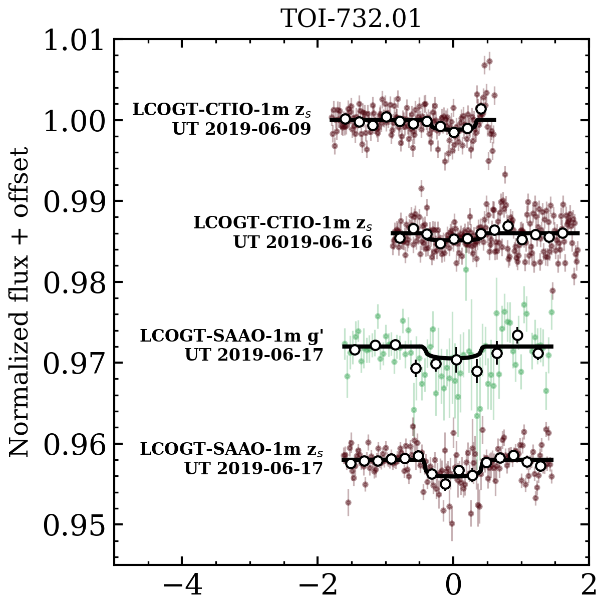
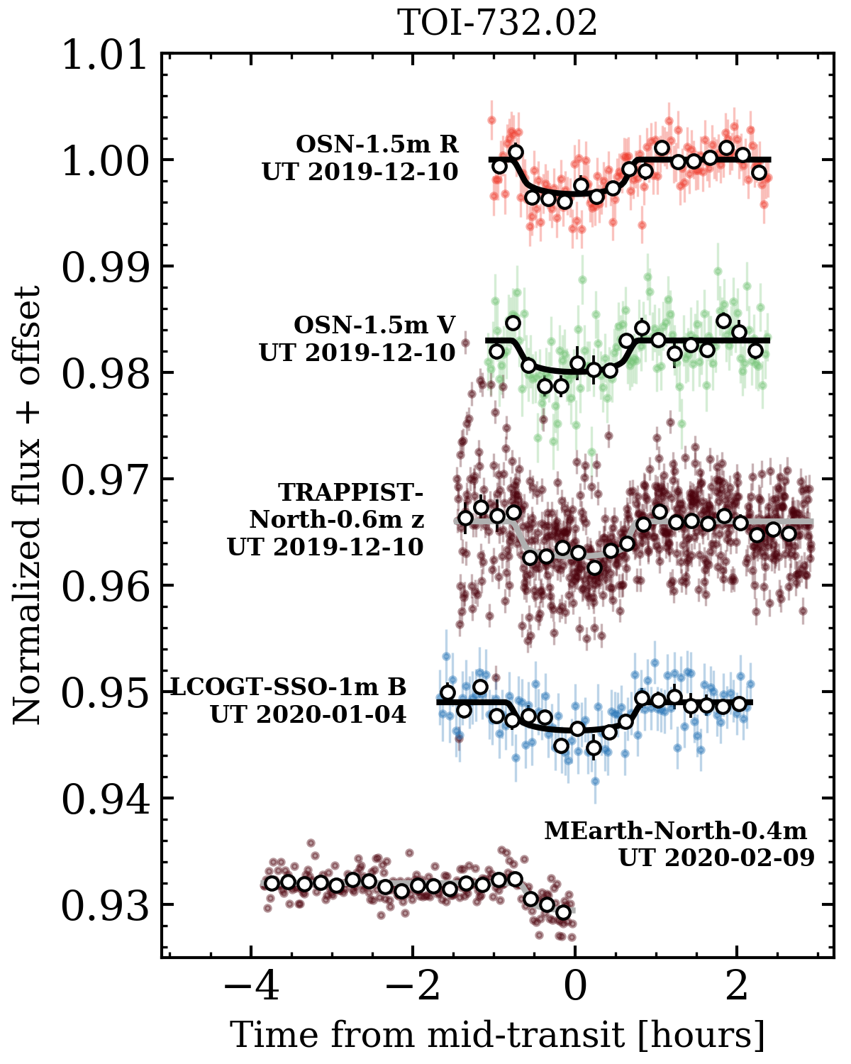
Numerous ground-based facilities conducted photometric follow-up of the TOI-732 system. Their respective data acquisition and reduction strategies are described in the following sections while their detrended light curves are plotted in Figure 2. Differences in the instrumental setups and nightly observing conditions produce varying levels of photometric precision among the light curves. Each detrended light curve, available through TFOP, is fit with a Mandel & Agol (2002) transit model that we calculate using the batman software package (Kreidberg, 2015). The shallow transit depths of both planet candidates produce low S/N transit light curves that may only marginally improve the measurement precision on most model parameters compared to the values measured from the TESS light curve with the exception being the planets’ orbital periods when all light curves are fit simultaneously. As such, we fix the orbital periods and impact parameters in the individual light curve fits to the values obtained from the SPOC Data Validation module ($P_{b}=0.76842$ days, $P_{c}=12.25422$ days, $b_{b}=0.69$, $b_{c}=0.35$). We also derive the scaled semimajor axes using the stellar parameters given in Table 1 ($a_{b}/R_{s}=6.96,a_{c}/R_{s}=44.09$). Each planet’s orbit is also fixed to circular and the quadratic limb darkening parameters in the corresponding passband are interpolated from the Claret & Bloemen (2011) tables using the EXOFAST software (Eastman et al., 2013) given LTT 3780’s $T_{\text{eff}}$, $\log{g}$, and [Fe/H]. We fit the following parameters via non-linear least squares optimization using scipy.curve_fit: the baseline flux $f_{0}$, the time of mid-transit $T_{0}$, and the planet-to-star radius ratio $r_{p}/R_{s}$. Measuring $T_{0}$ relative to the expected transit time is used to refine the planet’s orbital ephemeris while $r_{p}/R_{s}$ measurements in each passband are required to investigate transit depth chromaticity as a chromatically varying transit depth could be indicative of a blended EB.

Figure 2: Ground-based transit light curves of TOI-732.01 (upper panel) and 02 (lower panel) taken as part of TFOP. Solid curves depict the optimized transit model fit with all model parameters fixed other than the baseline flux, the mid-transit time, and the planet-to-star radius ratio. Annotated next to each light curve is the telescope facility, the passband, and the UT observation date.

3.3.1 LCOGT photometry

We used three observatories as part of the Las Cumbres Observatory Global Telescope network (LCOGT; Brown et al., 2013) to follow-up transits of both TOI-732.01 and 02. Each 1m telescope is equipped with a $4096\times 4096$ LCOGT SINISTRO camera whose pixel scale is 389 mas pixel^-1, resulting in a $26^{\prime}\times 26^{\prime}$ field-of-view (FOV). We calibrated all image sequences using the standard LCOGT BANZAI pipeline (McCully et al., 2018). An example of one such image from the LCOGT was shown in Figure 1.

We observed three full transits of TOI-732.01 between UT June 9-17, 2019 from various LCOGT observatories. These data include two $z_{s}$-band light curves taken at the LCOGT-Cerro Tololo Inter-American Observatory (CTIO) on UT June 9 and 16 2019, and a third transit light curve obtained on UT June 17, 2019 in the $z_{s}$ and $g^{\prime}$-bands by the LCOGT-South African Astronomical Observatory (SAAO). These four light curves are shown in Figure 2. We searched for transit-like events from nearby EBs (NEB) around 37 sources identified by Gaia DR2 to be within $2.5^{\prime}$. The field was consequently cleared of NEBs down to $\Delta z_{s}=7.686$ as no transit-like signals were detected on any off-target source. All three expected transit events were shown to occur on-target and arrived within 4 minutes of their expected transit times.

We observed one full transit of TOI-732.02 on UT January 4, 2020 with the LCOGT-Siding Springs Observatory (SSO) in the $B$-band. The light curve is included in Figure 2. Similarly to our TOI-732.01 transit analysis, the field was cleared of NEBs during the TOI-732.02 transit window. The expected transit event was shown to occur on-target with a transit depth of 2.4 parts per thousand (ppt). However, the transit arrived 60 minutes early indicating that the preliminary orbital period of $P_{c}=12.254$ days, derived from the TESS light curve alone, is slightly underestimated if the period is constant. The orbital period of LTT 3780c will be refined in our global analysis in Sect. 4, which will include the ground-based light curves.

3.3.2 OSN photometry

We observed one additional transit of TOI-732.02 on UT December 10, 2019 with the Observatorio de Sierra Nevada (OSN) 1.5m telescope near Granada, Spain. The OSN 1.5m telescope is equipped with an Andor ikon-L $2048\times 2048$ CCD camera whose pixel scale is 232 mas pixel^-1, resulting in a $7.9^{\prime}\times 7.9^{\prime}$ FOV. We observed the full transit simultaneously in both the $V$ and $R$-bands to check for chromaticity. Similarly to the LCOGT-SSO transit observation of TOI-732.02, the expected transit event arrived 60 minutes early. The measured transit depths of 2.9 ppt and 3.2 ppt in the $V$ and $R$-bands respectively are consistent with each other and with the LCO-SSO $B$-band transit at $1\sigma$. TOI-732.02 therefore does not show any strong chromaticity. The two transit light curves are included in Figure 2.

3.3.3 TRAPPIST-North photometry

The UT December 10, 2019 transit of TOI-732.02 observed by OSN was also observed by the 60cm TRAnsiting Planets and PlanetesImals Small Telescope-North (TRAPPIST-North) located at the Oukaïmden Observatory in Morocco (Jehin et al., 2011; Gillon et al., 2013; Barkaoui et al., 2019). TRAPPIST-North employs a $2048\times 2048$ pixel Andor IKONL BEX2 DD camera with a pixel scale of 600 mas pixel^-1 resulting in a $20.5^{\prime}\times 20.5^{\prime}$ FOV. The photometry was analyzed using custom software for TRAPPIST-North. We observed the full transit in the $z$-band, thus contributing to the four transit light curves of TOI-732.02 from TFOP in the $B$, $V$, $R$, and $z$-bands. The measured transit depth in the $z$-band is 3.2 ppt, which is consistent with the measured transit depths in the aforementioned passbands thus confirming that no strong chromaticity is detected. The TRAPPIST-North light curve is included in Figure 2.

3.3.4 MEarth-North photometry

We observed a partial transit of TOI-732.02 on UT February 9, 2020 using seven of eight telescopes from the MEarth-North telescope array located at FLWO on Mount Hopkins, AZ. The MEarth-North array consists of eight 40cm Ritchey-Chrétien telescopes, each equipped with a $2048\times 2048$ pixel Apogee U42 camera. The 750 mas pixel scale results in a $25.6^{\prime}\times 25.6^{\prime}$ FOV. The light curve was obtained in the custom MEarth passband centered in the red optical and is shown in Figure 2. The observations include a three hour out-of-transit baseline plus the transit ingress and 37 minutes in-transit, equal to nearly half of the full transit duration. The measured transit depth of 3.3 ppt is consistent with all other TFOP transits again confirming the lack of transit depth chromaticity.

The collective photometric data from TFOP have verified the periodic nature of the transits of TOI-732.01 and 02 and that both of these planet candidates orbit the target star LTT 3780. We do not detect any significant depth discrepancies, indicating that the transits are likely achromatic and thus consistent with being planetary in origin. Furthermore, the early arrival of the TOI-732.02 transits on December 10, 2019 and on January 4, 2020 allow us to estimate the true orbital period of LTT 3780c, which shrinks from its SPOC-reported value of 12.254 to 12.2519 days, assuming a constant period. This refined period prior is used in our up-coming analysis of the TESS light curve in Sect. 4.1.

3.4 High-resolution imaging

Very nearby stars that are not detected in Gaia DR2, nor in any of the seeing-limited image sequences, and that fall within the same $21^{\prime\prime}$ TESS pixel as the target star, will result in photometric contamination that is unaccounted for in the TESS light curve. This effect reduces the depth of the observed transits and can produce a false positive transit signal from another astrophysical source, such as a blended EB (Ciardi et al., 2015). We used two independent sets of high-resolution follow-up imaging sequences to search for any such close-in sources as described in the following sections.

3.4.1 SOAR speckle imaging

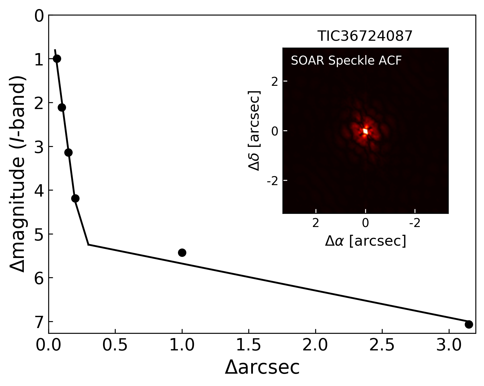
We obtained SOAR speckle imaging (Tokovinin, 2018) of LTT 3780 on UT December 12, 2019 in the $I$-band, a visible bandpass similar to that of TESS. Details of the observations from the SOAR TESS survey are provided in Ziegler et al. (2020). No bright nearby stars are detected within $3^{\prime\prime}$ of LTT 3780 within the $5\sigma$ detection sensitivity of the observations. The resulting $5\sigma$ contrast curve is plotted in Figure 3 along with the speckle auto-correlation function.

Figure 3: Upper panel: $I$-band $5\sigma$ contrast curve from SOAR speckle imaging of LTT 3780 (TIC 36724087). The inset depicts the corresponding speckle auto-correlation function. Lower panel: Br$\gamma$ $5\sigma$ contrast curve from Gemini/NIRI AO imaging. A few bad pixels persist at $2^{\prime\prime}$ from the target (blue diamond), but these have a minimal effect on the contrast. The inset depicts the central coadded image centered on LTT 3780. No visual companions are detected in either dataset at $\geq 5\sigma$.

3.4.2 NIRI AO imaging

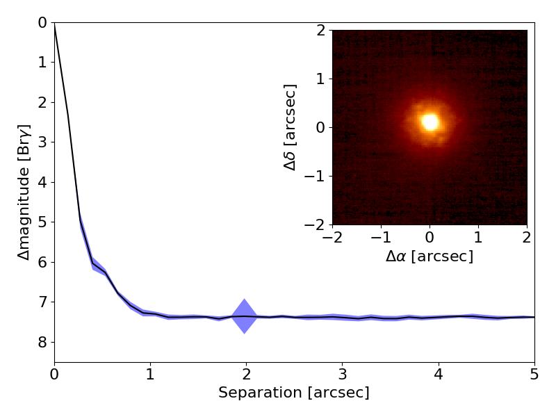
We obtained adaptive-optics (AO) images with Gemini/NIRI (Hodapp et al., 2003) on UT November 25, 2019 in the Br$\gamma$ filter (2.17 $\mu$m). We collected nine dithered images with integration times of 2.2 seconds. We followed a standard data reduction procedure including corrections for bad pixels, flat-fielding, sky background subtraction, and image coaddition. No visual companions are identified within $5^{\prime\prime}$ of LTT 3780 within the $5\sigma$ sensitivity of the observations. These high quality data are sensitive to companions five magnitudes fainter than the target at just 270 mas and 7.4 magnitudes fainter at separations $\gtrsim 1^{\prime\prime}$. The $5\sigma$ contrast curve and the coadded image centered on LTT 3780 are included in Figure 3.

Due to the single-lined spectrum of LTT 3780, the verification of the expected transit events on-target from ground-based photometry, and the lack of nearby contaminating sources from high-resolution imaging, we conclude that the planet candidates TOI-732.01 and 02 are verified planets. We will refer to these planets as LTT 3780b and c for the remainder of this study.

3.5 Precise radial-velocities

3.5.1 HARPS radial velocities

We obtained 33 spectra of LTT 3780 with the High Accuracy Radial velocity Planet Searcher (HARPS; Mayor et al., 2003) échelle spectrograph mounted at the ESO 3.6m telescope at La Silla Observatory, Chile. The HARPS optical spectrograph at $R=115,000$ is stabilized in pressure and temperature, which enable it to achieve sub-m s^-1 accuracy. The observations were taken between UT June 21, 2019 and February 24, 2020 as part of the ESO program 1102.C-0339. The exposure time was set to 2400 seconds, which resulted in a median S/N over all orders of 26 and a median measurement uncertainty of 1.31 m s^-1 following the RV extraction described below. Similarly to the TRES reconnaissance spectra at $R=44,000$, LTT 3780 does not exhibit any rotational broadening in the HARPS spectra. The corresponding upper limit on stellar rotation is $v\sin{i}$ $\leq 1.3$ km s^-1.

We extracted the HARPS RV measurements using the TERRA pipeline (Anglada-Escudé & Butler, 2012). TERRA employs a template-matching scheme that has been shown to outperform the cross-correlation function (CCF) technique on M dwarfs (Anglada-Escudé & Butler, 2012). M dwarfs are particularly well-suited to RV extraction via template-matching because the line lists used to define the binary mask for the CCF technique are incomplete. The resulting CCF template is often a poor match for cool M dwarfs.

TERRA constructs a master template spectrum by first shifting the individual spectra to the barycentric frame using the barycentric corrections calculated by the HARPS Data Reduction Software (DRS; Lovis & Pepe, 2007). We masked portions of the wavelength-calibrated spectra in which telluric absorption exceeds 1%. The spectra are then coadded to build a high S/N spectral template. We computed the RV of each spectrum by least-squares matching the individual spectrum to the master template. Throughout the extraction process, we only consider orders redward of order 18 (428-689 nm) such that the bluest orders at low S/N are ignored. Because the master spectrum is derived from the observed spectra, template construction does not require any additional assumptions about the stellar properties. Using this method, we found that the median LTT 3780 RV measurement precision was improved by a factor of two compared to the standard CCF method utilized within the HARPS DRS. The resulting RV time series is reported in Table 2.

Table 2: Radial velocity time series of LTT 3780 from HARPS & HARPS-N

Time	RV	$\sigma_{\text{RV}}$	Instrument
$[$BJD - 2,457,000$]$	$[\text{m s}^{-1}]$	$[\text{m s}^{-1}]$
1821.837965	-0.959	1.310	HARPS
1831.760260	-10.056	1.330	HARPS-N
1836.858657	-5.946	1.403	HARPS

3.5.2 HARPS-N radial velocities

We obtained 30 spectra of LTT 3780 with the HARPS-N optical échelle spectrograph at the TNG on La Palma in the Canary Islands. The observations were taken as part of the HARPS-N Collaboration Guaranteed Time Observations program between UT December 14, 2019 and March 15, 2020. The exposure time was set to 1800 seconds, which resulted in a median S/N over all orders of 20 and a median measurement uncertainty of 1.43 m s^-1.

Identically to the HARPS RVs, we extracted the HARPS-N RVs using the TERRA template-matching algorithm. The resulting RV time series is included in Table 2.

4 Data Analysis & Results

Here we conduct two independent analyses of our data to test the robustness of the recovered planetary parameters. In our fiducial analysis (Sects. 4.1 and 4.2), the TESS light curve is modeled separately with the resulting planet parameters being used as priors in the subsequent RV analysis. In Sect. 4.3 we describe an alternative, global analysis using the EXOFASTv2 software (Eastman et al., 2019).

4.1 TESS transit analysis

We begin by analyzing the TESS PDCSAP light curve wherein the planet candidates TOI-732.01 and 02 were initially detected. The majority of apparent signals from non-random noise sources in the light curve have already been removed by the SPOC processing. However, low frequency and small amplitude signals that do not resemble planetary transits are seen to persist in the PDCSAP light curve shown in Figure 4. The nature of these signals as residual systematics or photometric stellar variability is unclear so we proceed with modeling the aforementioned noise signals as an untrained semi-parametric Gaussian process (GP) regression model, simultaneously with the two transiting planet candidates using the exoplanet software package (Foreman-Mackey et al., 2019). exoplanet computes analytical transit models using the STARRY package (Luger et al., 2019) and uses the celerite package (Foreman-Mackey et al., 2017) to evaluate the marginalized likelihood under a GP model. In this analysis, the covariance kernel takes the form of a stochastically-driven, damped simple harmonic oscillator (SHO) whose Fourier transform is known as the power spectral density (PSD) and is given by

Figure 4: Upper panel: the TESS PDCSAP light curve of LTT 3780 (black curve) along with the mean GP detrending model (green curve) and its $3\sigma$ confidence interval in the surrounding shaded region which is narrow and hence difficult to discern. The vertical red and blue ticks along the x-axis highlight the mid-transit times of the planets LTT 3780b and c respectively. Middle panel: the detrended TESS light curve. Lower panels: phase-folded light curves of LTT 3780b (left) and c (right) along with their best-fit transit models. White markers depict the temporally-binned phase-folded light curves to help visualize the transit events.

$$S(\omega)=\sqrt{\frac{2}{\pi}}\frac{S_{0}\,\omega_{0}^{4}}{(\omega^{2}-{\omega_{0}}^{2})^{2}+{\omega_{0}}^{2}\,\omega^{2}/Q^{2}}.$$ (1)

The PSD of the SHO is parameterized by the frequency of the undamped oscillator $\omega_{0}$, $S_{0}$, which is proportional to the power at the frequency $\omega_{0}$, and the quality factor $Q$, which is fixed to $\sqrt{0.5}$. We selected this covariance kernel and parameterization because working in Fourier space is much more computationally efficient for large datasets, such as our TESS light curve ($N=15,210$), and because the underlying cause of the photometric variations being modeled remains unknown. In practice, we also fit for the baseline flux $f_{0}$ and an additive scalar jitter $s_{\text{TESS}}$. We fit the GP hyperparameters using the parameter combinations $\{\ln{\omega_{0}},\ln{S_{0}\omega_{0}^{4}},f_{0},\log{s_{\text{TESS}}^{2}}\}$ with uninformative priors.

The transit model within exoplanet fits the stellar mass $M_{s}$, stellar radius $R_{s}$, and quadratic limb darkening parameters $\{u_{1},u_{2}\}$ along with the following planetary parameters: logarithmic orbital periods $\ln{P}$, times of mid-transit $T_{0}$, logarithmic planet radii $\ln{r_{p}}$, impact parameters $b$, and the eccentricity and argument of periastron of LTT 3780c only; $\{e_{c},\omega_{c}\}$. We assume a circular orbit for the inner planet LTT 3780b because its ultra-short period of 0.77 days implies a very short circularization timescale of $\ll 1$ Myr (Goldreich & Soter, 1966). Jointly fitting for the physical stellar and planetary parameters enables us to derive the transit observables $a/R_{s}$, $r_{p}/R_{s}$, and inclination $i$. The joint GP plus two-planet transit model therefore includes 18 model parameters: $\{f_{0},\ln{\omega_{0}},\ln{S_{0}\omega_{0}^{4}},\ln{s_{\text{TESS}}^{2}},M_{s},R_{s},$ $u_{1},u_{2},\ln{P_{b}},T_{0,b},\ln{r_{p,b}},b_{b},\ln{P_{c}},T_{0,c},\ln{r_{p,c}},b_{c},e_{c},\omega_{c}\}$. Table 3 summarizes the TESS transit model parameter priors used in this, our fiducial analysis.

Table 3: TESS light curve and RV model parameter priors

Parameter	Fiducial Model Priors	EXOFASTv2 Model Priors
Stellar parameters
$T_{\text{eff}}$, [K]	$\mathcal{N}(3331,157)$	$\mathcal{N}(3351,150)$
$M_{s}$, [M⊙]	$\mathcal{N}(0.401,0.012)$	$\mathcal{N}(0.401,0.012)$
$R_{s}$, [R⊙]	$\mathcal{N}(0.374,0.011)$	$\mathcal{N}(0.374,0.011)$
Light curve hyperparameters
$f_{0}$	$\mathcal{N}(0,10)$	$\mathcal{U}(-\inf,\inf)$
$\ln{\omega_{0}}$, [days-1]	$\mathcal{N}(0,10)$	-
$\ln{S_{0}\omega_{0}^{4}}$	$\mathcal{N}(\ln{\text{var}(\mathbf{f}_{\text{TESS}})},10)$	-
$\ln{s_{\text{TESS}}^{2}}$	$\mathcal{N}(\ln{\text{var}(\mathbf{f}_{\text{TESS}})},10)$	-
$u_{1}$	$\mathcal{U}(0,1)$	$\mathcal{U}(0.225,0.425)$
$u_{2}$	$\mathcal{U}(0,1)$	$\mathcal{U}(0.232,0.432)$
Dilution	-	$\mathcal{N}(0,0.1\>\delta)$
RV parameters
$\ln{\lambda}$, [days]	$\mathcal{U}(\ln{1},\ln{1000})$	-
$\ln{\Gamma}$	$\mathcal{U}(-3,3)$	-
$\ln{P_{\text{GP}}}$, [days]	$\mathcal{N}(\ln{104},\ln{30})$	-
$\ln{a}_{\text{HARPS}}$, [m s-1]	$\mathcal{U}(-5,5)$	-
$\ln{a}_{\text{HARPS-N}}$, [m s-1]	$\mathcal{U}(-5,5)$	-
$\ln{s}_{\text{HARPS}}$, [m s-1]	$\mathcal{U}(-5,5)$	$\mathcal{U}(-\inf,\inf)$
$\ln{s}_{\text{HARPS-N}}$, [m s-1]	$\mathcal{U}(-5,5)$	$\mathcal{U}(-\inf,\inf)$
$\gamma_{\text{HARPS}}$, [m s-1]	$\mathcal{U}(-185,205)$	$\mathcal{U}(-\inf,\inf)$
$\gamma_{\text{HARPS-N}}$, [m s-1]	$\mathcal{U}(-185,205)$	$\mathcal{U}(-\inf,\inf)$
LTT 3780b parameters
$\ln{P}_{b}$, [days]	$\mathcal{N}(\ln{0.768},0.5)$	-
$P_{b}$, [days]	-	$\mathcal{U}(-\inf,\inf)$
$T_{0,b}$, [BJD-2,457,000]	$\mathcal{N}(1543.911,0.5)$	$\mathcal{U}(1543.7,1544.2)$
$\ln{r_{p,b}}$, [R⊕]	$\mathcal{N}(0.5\cdot\ln(Z_{b})+\ln{R_{s}},1)$	-
$r_{p,b}/R_{s}$	-	$\mathcal{U}(-\inf,\inf)$
$b_{b}$	$\mathcal{U}(0,1+r_{p,b}/R_{s})$	-
$\ln{K}_{b}$, [m s-1]	$\mathcal{U}(-5,5)$	-
$K_{b}$, [m s-1]	-	$\mathcal{U}(-\inf,\inf)$
LTT 3780c parameters
$\ln{P}_{c}$, [days]	$\mathcal{N}(\ln{12.254},0.5)$	-
$P_{c}$, [days]	-	$\mathcal{U}(-\inf,\inf)$
$T_{0,c}$, [BJD-2,457,000]	$\mathcal{N}(1546.848,0.5)$	$\mathcal{U}(1542.8,1550.9)$
$\ln{r_{p,c}}$, [R⊕]	$\mathcal{N}(0.5\cdot\ln(Z_{c})+\ln{R_{s}},1)$
$r_{p,c}/R_{s}$	-	$\mathcal{U}(-\inf,\inf)$
$b_{c}$	$\mathcal{U}(0,1+r_{p,c}/R_{s})$
$\ln{K}_{c}$, [m s-1]	$\mathcal{U}(-5,5)$	-
$K_{c}$, [m s-1]	-	$\mathcal{U}(-\inf,\inf)$
$e_{c}$	$\mathcal{B}(0.867,3.03)$
$\omega_{c}$, [rad]	$\mathcal{U}(-\pi,\pi)$

Note. — Gaussian distributions are denoted by $\mathcal{N}$ and are parameterized by mean and standard deviation values. Uniform distributions are denoted by $\mathcal{U}$ and bounded by the specified lower and upper limits. Beta distributions are denoted by $\mathcal{B}$ and are parameterized by the shape parameters $\alpha$ and $\beta$.

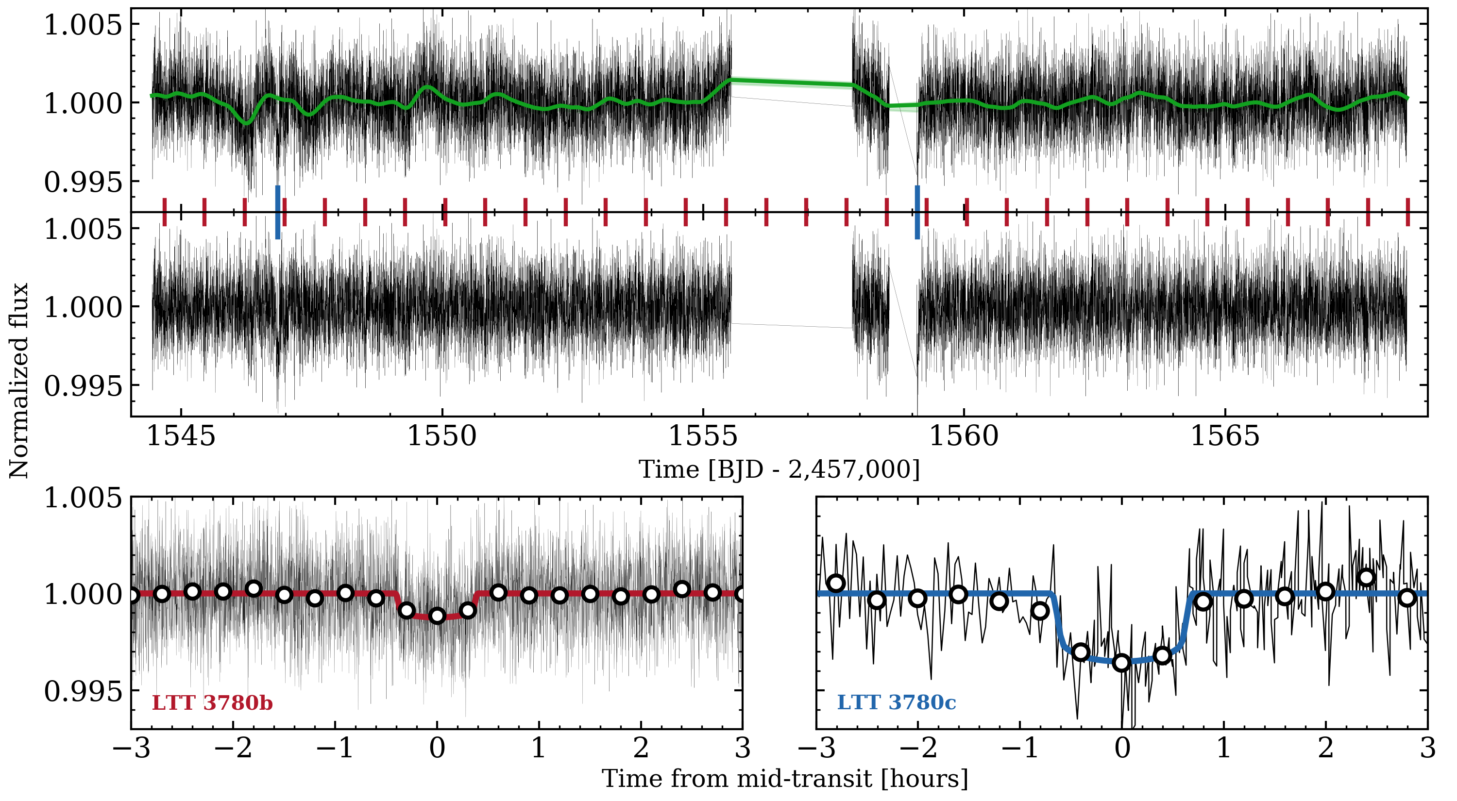
Our full model is fit to the TESS PDCSAP light curve using the PyMC3 Markov Chain Monte-Carlo (MCMC) package (Salvatier et al., 2016) implemented within exoplanet. We ran four simultaneous chains with 4000 tuning steps and 3000 draws in the final sample. PyMC3 produces the 18-dimensional joint posterior probability density function (PDF) of the model parameters. Median point estimates from the marginalized posterior PDFs of the GP hyperparameters are used to construct the GP predictive distribution whose mean function is shown in Figure 4 and is used to detrend the TESS light curve for visualization purposes. Similarly, the median point estimates of the transit model parameters are used to compute the ‘best-fit’ transit models shown in Figure 4. Table 6 reports the median values of all model parameters from their marginalized posterior PDFs along with their uncertainties from the $16^{\text{th}}$ and $84^{\text{th}}$ percentiles.

4.2 Precise radial-velocity analysis

In our fiducial analysis, we elected to fit the RVs independently of the transit data but exploiting the strong priors on the orbital periods and mid-transit times established by our TESS light curve analysis (Sect. 4.1). We note that the information content within the TESS light curve and the RV measurements with regards to their shared model parameters (i.e. $\{P_{b},T_{0,b},P_{c},T_{0,c},e_{c},\omega_{c}\}$) is dominated by one dataset or the other. In other words, the strongest constraints on each planet’s orbital period and mid-transit time are derived from the TESS and ground-based transit light curves. Conversely, most of the information regarding the eccentricity and argument of periastron of LTT 3780c is derived from the RVs since the planet’s secondary eclipse is unresolved in the TESS light curve and the eccentricity’s effect on the transit duration is degenerate with $a/R_{s}$, $r_{p}/R_{s}$, and $b$. Note that this is only an approximation as global transit plus RV modeling can help to mitigate the eccentricity degeneracy (Eastman et al., 2019). We will also consider a global model in Sect. 4.3.

Although LTT 3780 is known to be relatively inactive, we do not expect its surface to be completely static and homogeneous. As such, we expect some temporally-correlated residual RV signals from magnetic activity that we model with a quasi-periodic GP regression model for each spectrograph. The quasi-periodic covariance kernel is

$$k_{ij}=a^{2}\exp{\left[-\frac{(t_{i}-t_{j})^{2}}{2\lambda^{2}}-\Gamma^{2}\sin^{2}{\left(\frac{\pi|t_{i}-t_{j}|}{P_{\text{GP}}}\right)}\right]}$$ (2)

and features four hyperparameters: the covariance amplitude $a$, the exponential timescale $\lambda$, the coherence $\Gamma$, and the periodic timescale $P_{\text{GP}}$. We also fit an additive scalar jitter $s_{\text{RV}}$ for each spectrograph to absorb any excess white noise. Due to the unique systematic noise properties of each spectrograph, we fit a unique covariance amplitude and scalar jitter to the data from each of the HARPS and HARPS-N spectrographs. Throughout, the covariance parameters $\{\lambda,\Gamma,P_{\text{GP}}\}$, which only depend on signals originating from the star, are kept fixed between the two spectrographs.

Our full RV model consists of a GP activity model for each spectrograph plus independent Keplerian orbital solutions for each planet with RV semi-amplitudes $K_{b}$ and $K_{c}$. We also fit for each spectrograph’s systemic velocity $\gamma$ to account for any RV offset between the two instruments. Our full RV model therefore features 17 model parameters: $\{\ln{a}_{\text{HARPS}},\ln{a}_{\text{HARPS-N}},\ln{\lambda},\ln{\Gamma},\ln{P_{\text{GP}}},$ $\ln{s}_{\text{HARPS}},\ln{s}_{\text{HARPS-N}},\gamma_{\text{HARPS}},\gamma_{\text{HARPS-N}},$ $P_{b},T_{0,b},\ln{K_{b}},$ $P_{c},T_{0,c},\ln{K_{c}},h_{c},k_{c}\}$ where $h_{c}=\sqrt{e_{c}}\cos{\omega_{c}}$ and $k_{c}=\sqrt{e_{c}}\sin{\omega_{c}}$. Note that the GP hyperparameters, scalar jitter parameters, and planetary semi-amplitudes are fit in logarithmic units. Table 3 includes each of the RV model parameter priors.

Figure 5: The RV data and individual model components from our analysis of the HARPS (gray circles) and HARPS-N (green triangles) RV measurements. The data and models are depicted in the left column of the first five rows while their corresponding Bayesian generalized Lomb-Scargle periodograms are depicted in the right column. The marginalized posteriors of the LTT 3780b and c orbital periods are depicted as vertical lines along with the estimated stellar rotation period using the M dwarf activity-rotation relation from Astudillo-Defru et al. (2017) ($P_{\text{rot}}$ $=104\pm 15$ days). First row: the raw RV measurements. Second row: the RV activity signal modeled with a quasi-periodic GP for each spectrograph. Third row: the RV signal from LTT 3780b at 0.77 days. Fourth row: the RV signal from LTT 3780c at 12.25 days. Fifth row: the RV residuals. Bottom row: the phase-folded RV signals of LTT 3780b and c.

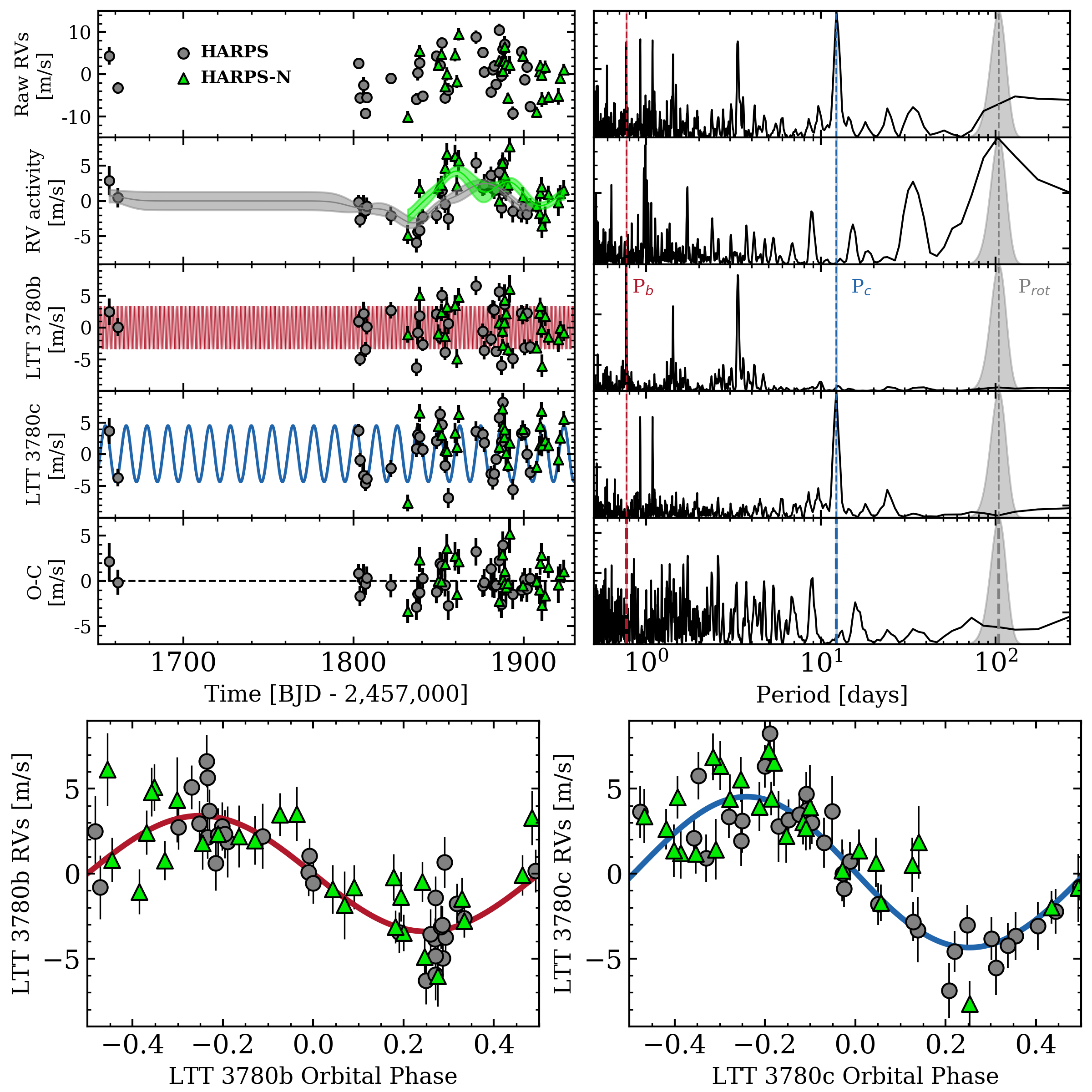
Figure 5 shows the raw RVs and the individual model components including the RV activity along with LTT 3780b and c. The Bayesian generalized Lomb-Scargle periodogram (BGLS; Mortier et al., 2015) of each RV component is also included in Figure 5. The BGLS of the raw RVs exhibits a small number of significant peaks (e.g. 3.1 days) that are not strictly at either planet’s orbital period. We will see that the subtraction of the individual Keplerian orbits effectively removes these periodicities such that they can be attributed to harmonics of the planetary orbital periods. The median RV model parameters from their marginalized posterior PDFs are used to produce the models shown in Figure 5 and are reported in Table 6 along with their $16^{\text{th}}$ and $84^{\text{th}}$ percentiles. The RV semi-amplitudes of LTT 3780b and c are found to be $3.41^{+0.63}_{-0.63}$ and $4.44^{+0.82}_{-0.68}$ m s^-1 and thus are clearly detected at $5.4\sigma$ and $5.9\sigma$ respectively. The resulting Keplerian RV signals are clearly discernible in their phase-folded RV time series. The rms of the RV residuals are found to be 1.55 and 1.74 m s^-1 for HARPS and HARPS-N respectively.

M dwarfs are known to commonly host 2-3 planets per star out to 200 days (e.g. Dressing & Charbonneau, 2015; Ballard & Johnson, 2016; Cloutier & Menou, 2020; Hardegree-Ullman et al., 2019) such that the probability that a third planet exists around LTT 3780 is non-negligible. However, the BGLS of the RV residuals in Figure 5 does not exhibit any strong periodic signals that are statistically significant. This indicates that a hypothetical third planet is unlikely to have been detected. To confirm this robustly, we considered a three-planet RV model, with fixed Keplerian parameters for LTT 3780b and c, plus a third Keplerian component ‘d’ on a circular orbit. We separately tested two three-planet models with differing priors on the orbital period $P_{d}$: $\mathcal{U}(1.3,2.1)$ and $\mathcal{U}(50,150)$ days. The chosen period limits approximately span the two highest peaks in the BGLS of the RV residuals. We then ran two separate MCMCs to sample the posteriors of the hypothetical planet’s period, time of inferior conjunction (analogous to the mid-transit time), and semi-amplitude. We find that neither model settles onto a preferred period or phase and each marginalized $P_{d}$ posterior simply recovers its uninformative prior. The lack of a well-defined maximum a-posteriori $P_{d}$ and $T_{0,d}$ prevents us from searching the TESS light curve for any missed transit signals from the hypothetical planet ‘d’ and from placing a meaningful upper limit on the planet’s mass. We note that the only threshold crossing events identified by the TPS in the TESS light curve were those corresponding to the confirmed planets LTT 3780b and c. Additionally, the recovered semi-amplitudes $K_{d}$ in both MCMCs favored zero m s^-1 with an upper limit of $K_{d}\leq 2.4$ m s^-1 at 95% confidence. Taken together, these findings emphasize that the fiducial two-planet model for the current dataset is likely complete as no third planet is detected in our data.

4.3 An alternative global transit + RV analysis

To evaluate the robustness of the results derived in our fiducial analysis (Sects. 4.1 and 4.2), we conducted an independent analysis using the EXOFASTv2 exoplanet transit plus RV fitting package (Eastman et al., 2019). The methods of the EXOFASTv2 fitting routine are detailed in Eastman et al. (2019) although we provide a brief summary here.

To constrain the stellar-dependent parameters during the transit fit, we feed EXOFASTv2 the $M_{s}$ and $R_{s}$ parameter priors as in our fiducial model. The routine also takes as input the pre-detrended light curves from TESS and from ground-based facilities, and performs a differential MCMC to evaluate the two-planet transit model whose parameter priors are included in Table 3.

There are a few notable differences between our fiducial analysis (Sects. 4.1 and 4.2) and the EXOFASTv2 approach. The exoplanet model simultaneously fits the hyperparameters of the GP detrending model plus the transiting planet parameters to achieve self-consistent detrending and transit models wherein the uncertainties in the recovered planet parameters are marginalized over uncertainties in the detrending model. Conversely, EXOFASTv2 uses pre-detrended light curves and so the aforementioned marginalization of the planet parameter uncertainties over the GP hyperparameters does not occur. Furthermore, the RV model in our fiducial analysis includes the treatment of residual RV signals as a quasi-periodic GP whereas, EXOFASTv2 assumes the RV residuals to be well-represented by a Gaussian noise term characterized by an additive jitter factor.

Our EXOFASTv2 modeling has the important advantage of evaluating a global model that includes the TESS light curve, ground-based transit light curves, and RV measurements. The resulting planet parameters, including the orbital periods, mid-transit times, eccentricities, and argument of periastron, will therefore be self-consistent between all input datasets. In particular, each planet’s ephemeris will be more precisely constrained by the inclusion of the ground-based transit light curves and the eccentricity of LTT 3780c will be jointly constrained by its transit duration, Keplerian RV model, and the stellar density. EXOFASTv2 also fits a free dilution parameter to model any discrepancies between the dilution applied to the PDCSAP light curve and the true dilution.

The results from our fiducial model in Table 6 are accompanied by the results from our alternative analysis using EXOFASTv2. We find consistency between the two models at $<1\sigma$ for nearly all model parameters. This speaks to the robustness of the planetary model parameters inferred from our data. The only exceptions are the $2\sigma$ and $2.8\sigma$ discrepant RV jitter parameters $s_{\text{HARPS}}$ and $s_{\text{HARPS-N}}$. However, this is not alarming as the RV residuals, following the removal of the two Keplerian solutions, are modeled with a GP in our fiducial model whereas the EXOFASTv2 model treats the residuals with a scalar jitter. Crucially, these approaches yield consistent RV semi-amplitudes for LTT 3780b and c whose agreement between the two models is $0.2\sigma$ and $0.7\sigma$ respectively.

5 Discussion

5.1 Fundamental planet parameters

From our analysis of the TESS transit light curve we measure the planetary radii of LTT 3780b and c to be $r_{p,b}=1.332^{+0.072}_{-0.075}$ R_⊕ and $r_{p,c}=2.30^{+0.16}_{-0.15}$ R_⊕. By combining the TESS analysis with the mid-transit times measured from transit follow-up observations, we measure orbital periods for LTT 3780b and c to be $P_{b}=0.7683881^{+0.0000084}_{-0.0000083}$ days and $P_{c}=12.252048^{+0.000060}_{-0.000059}$ days. This places LTT 3780b at 0.012 AU where it receives 106 times Earth’s insolation. Assuming uniform heat redistribution and a Bond albedo of zero, LTT 3780b has an equilibrium temperature of $T_{\text{eq},b}=892$ K. Similarly, the orbital period of LTT 3780c places it at 0.077 AU where it receives 2.6 times Earth’s insolation with a zero-albedo equilibrium temperature of 353 K.

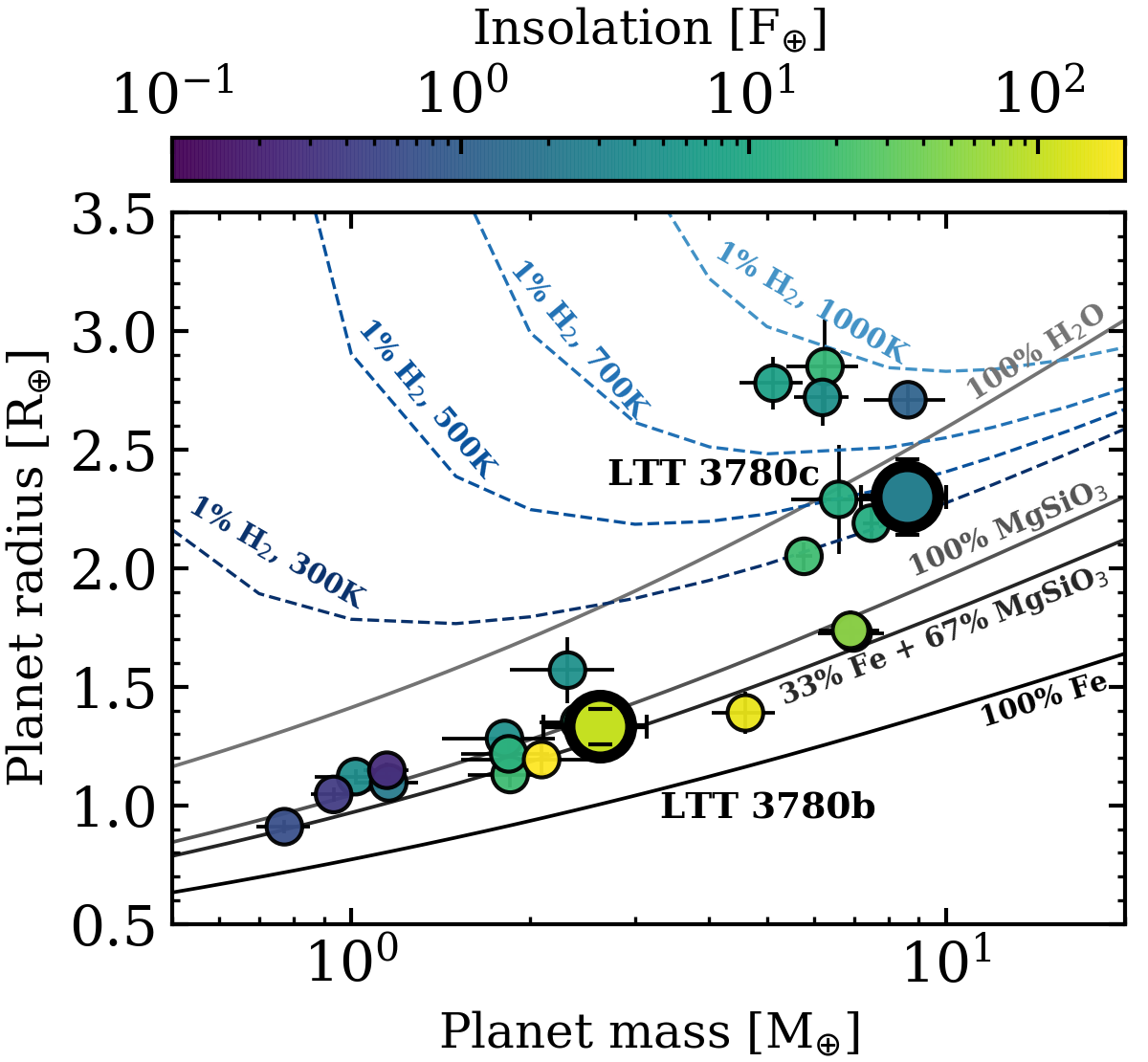
From our RV analysis we measure planet masses of $m_{p,b}=2.62^{+0.48}_{-0.46}$ M_⊕ and $m_{p,c}=8.6^{+1.6}_{-1.3}$ M_⊕, which represent $5.6\sigma$ and $5.9\sigma$ mass detections respectively. By combining the planetary mass and radius measurements, we derive bulk densities of $\rho_{p,b}=6.1^{+1.8}_{-1.5}$ g cm^-3 and $\rho_{p,c}=3.9^{+1.0}_{-0.9}$ g cm^-3. Figure 6 details the mass-radius diagram of exoplanets around M dwarfs with masses measured at the level of $\geq 3\sigma$, including the LTT 3780 planets. The LTT 3780 planet masses and radii are compared to theoretical models of fully-differentiated planetary interiors consisting of combinations of water, silicate rock, and iron (Zeng & Sasselov, 2013). In Figure 6 we see that LTT 3780b is consistent with an Earth-like bulk composition of 33% iron plus 67% magnesium silicate by mass. This composition is shared by the majority of planets in the $\lesssim 1.5$ R_⊕ size regime. We also consider models of Earth-like solid cores that include 1% H₂ envelopes by mass, over a range of equilibrium temperatures from 300-1000 K (Zeng et al., 2019). The mass and radius of LTT 3780c appear consistent with a water-dominated bulk composition but also with a predominantly Earth-like body that hosts an extended low mean molecular weight atmosphere. Distinguishing between these two degenerate structure models will require the extent of LTT 3780c’s atmosphere to be investigated through transmission spectroscopy. Due to the dependence of the atmospheric scale height on the planet’s surface gravity, the accurate interpretation of forthcoming transmission spectroscopy observations will be facilitated by the planetary mass measurements presented in this study. The feasibility of targeting LTT 3780c with transmission spectroscopy is discussed in Sect. 5.4.

Figure 6: Planetary mass-radius diagram for small planets orbiting M dwarfs including LTT 3780b and c (bold symbols). The solid curves represent planetary internal structure models for bodies composed of 100% water, 100% silicate rock, 67% rock plus 33% iron (i.e. Earth-like), and 100% iron by mass. The dashed curves represent models of planets with Earth-like solid cores plus a 1% by mass gaseous H₂ envelope at 1 mbar surface pressure and with the equilibrium temperature annotated next to each curve. Marker colors indicate the planet’s insolation.

The LTT 3780 two-planet system adds to the growing number of confirmed multi-planet systems around nearby M dwarfs with at least one transiting planet (e.g. GJ 1132; Berta-Thompson et al. 2015; Bonfils et al. 2018, K2-3; Crossfield et al. 2015; Damasso et al. 2018, K2-18; Montet et al. 2015; Cloutier et al. 2019b, L 98-59; Kostov et al. 2019; Cloutier et al. 2019a, LHS 1140; Dittmann et al. 2017; Ment et al. 2019, LP 791-18; Crossfield et al. 2019, TOI-270; Günther et al. 2019, TOI-700; Gilbert et al. 2020; Rodriguez et al. 2020, TRAPPIST-1; Gillon et al. 2017). With their sub-Neptune-sized radii and measured masses presented herein, both LTT 3780b and c contribute directly to the completion of the TESS level one science requirement to obtain masses for fifty planets smaller than 4 R_⊕.

5.2 Implications for the origin of the radius valley around mid-M dwarfs

The occurrence rate distribution of close-in planet radii around Sun-like stars features a bimodality with a dearth of planets at $1.7-2.0$ R_⊕ known as the radius valley (Fulton et al., 2017; Mayo et al., 2018). This feature likely results from the existence of a transition between predominantly rocky planets and larger planets that host significant H/He envelopes, as a function of planet radius and orbital separation. The slope of the radius valley in $P-r_{p}$ space marks the critical radius separating rocky and non-rocky planets as a function of orbital period. The empirical slope of the radius valley around Sun-like stars is consistent with models of thermally-driven atmospheric mass loss such as photoevaporation and core-powered mass loss (Van Eylen et al., 2018; Martinez et al., 2019; Wu, 2019). However for mid-K to mid-M dwarfs, the radius valley slope flattens and becomes increasingly favored by models of an alternative formation pathway for terrestrial planets in a gas-poor environment (CM20).

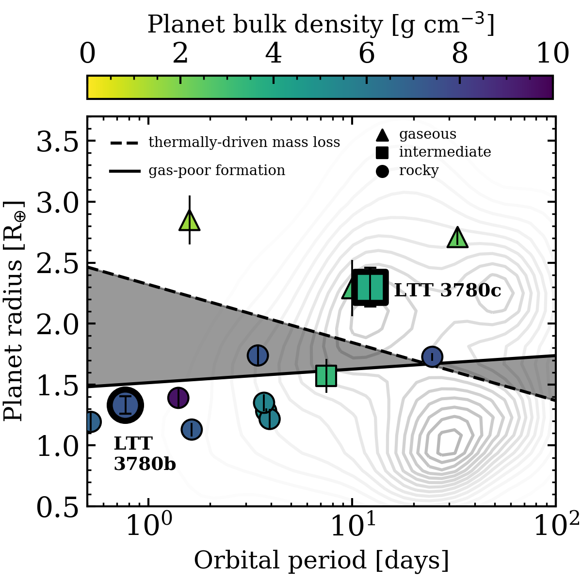
Figure 7 depicts the LTT 3780 planets in $P-r_{p}$ space, along with the subset of M dwarf planets from Figure 6 with RV-derived masses. The planets in Figure 7 are classified as having a bulk composition that is either rocky, gaseous, or intermediate based on their mass and radius. Rocky planets are defined as planets that are consistent with having a bulk density greater than that of 100% MgSiO₃ given their size. Similarly, unambiguously gaseous planets are defined as planets that are consistent with having a bulk density less than that of 100% H₂O given their size. The remaining planets are flagged as having bulk compositions that are intermediate between rocky and gaseous. LTT 3780b and c have rocky and intermediate dispositions respectively (Figure 6).

In Figure 7, LTT 3780b and c are shown to span the empirically-derived location of the radius valley around low mass stars under the gas-poor formation and photoevaporation models (CM20). The slope of the radius valley around low mass stars is considerably flatter than around Sun-like stars, with the former slope being consistent with gas-poor formation while the latter is more consistent with a thermally-driven atmospheric mass loss process. To compare the compositions of planets around low mass stars to the rocky/non-rocky transition locations in Figure 7, we scale the transition measured around Sun-like stars down to the low stellar mass regime under the photoevaporation model ($r_{p}\propto(M_{s}/M_{\odot})^{1/4}$; Wu, 2019). The slope measured around low mass stars is plotted verbatim in Figure 7. Both models predict that LTT 3780b should have a rocky bulk composition in which any residual gaseous envelope only contributes marginally to the planet’s mass and radius. Indeed these predictions are consistent with our finding that LTT 3780b has an Earth-like composition. Similarly, both models predict that LTT 3780c should be non-rocky in that it should have retained a substantial gaseous envelope and therefore be inconsistent with having a bulk rocky composition. Although we cannot definitively identify the bulk composition of LTT 3780c with our data, due to internal structure model degeneracies, we confirm that LTT 3780c is consistent with both model predictions. In other words, the models correctly identify LTT 3780c as being inconsistent with an Earth-like composition and requires a significant amount of volatile material or H/He gas to explain its mass and radius.

Figure 7: Period, radii, and bulk densities of M dwarf planets with precise RV masses compared to the empirical location of the radius valley around low mass stars versus orbital period and planet radius. LTT 3780b and c are depicted with the bold symbols. Contours represent the planetary occurrence rates around low mass stars (CM20). Planet marker shapes depict the planet’s compositional disposition as either rocky (circles), gaseous (triangles), or intermediate (squares). Marker colors indicate the planet’s bulk density. The dashed and solid lines depict the locations of the radius valley around low mass stars from model predictions of thermally-driven atmospheric mass loss and from gas-poor terrestrial planet formation respectively. The shaded regions highlight where the model predictions of planetary bulk compositions are discrepant between the two models.

5.2.1 Planetary mass limits from photoevaporation models

Stars such as LTT 3780 with multi-transiting planets that span the radius valley provide valuable test cases of radius valley emergence models. The virtue of these systems is that limits on the planetary masses can be derived by scaling the properties of one planet to the other (Owen & Campos Estrada, 2020). For example, assuming that the initial H/He envelope of the rocky planet below the valley has been completely stripped by some physical process, the theoretical minimum mass of the non-rocky planet above the valley can be calculated by scaling its properties to those of the rocky planet. An equivalent principle can be used to derive the maximum mass of the rocky planet. The power of this comparative scaling of planets within the same planetary system is that certain unobservable quantities that directly affect final planet masses are scaled out. An example of this is the host star’s XUV luminosity history in the photoevaporation scenario (Owen & Campos Estrada, 2020).

A full derivation is presented in Appendix A but here we simply state the condition for the consistency of the gaseous (i.e. non-rocky) and rocky planet parameters with the photoevaporation model. This requires that the gaseous planet’s mass loss timescale exceeds the maximum mass loss timescale of the rocky planet (Owen & Campos Estrada, 2020). This condition leads to

$$1\leq\frac{m_{\text{core,gas}}^{0.64}}{m_{\text{core,rock}}}\left(\frac{a_{\text{gas}}}{a_{\text{rock}}}\right)^{2/3}r_{\text{core,rock}}^{4/3}.$$ (3)

where each planet’s core mass and radius are given in units of the Earth. In the LTT 3780 system we define LTT 3780b to be the rocky planet below the valley whose H/He envelope has been photoevaporated away leaving behind a solid core whose mass and radius are equal to the planet’s total mass and radius: $m_{\text{core,rock}}=m_{p,b}=2.62\pm 0.47$ M_⊕ and $r_{\text{core,rock}}=r_{p,b}=1.332\pm 0.074$ R_⊕. The gaseous planet above the valley is then LTT 3780c, whose mass is assumed to be dominated by an Earth-like core such that $m_{\text{core,gas}}=m_{p,c}=8.6\pm 1.5$ M_⊕ and whose core radius is approximated by the mass-radius relation for Earth-like bodies ($r_{p}\propto m_{p}^{1/3.7}$; Zeng et al., 2016). Lastly, the semimajor axes $a_{\text{rock}}$ and $a_{\text{gas}}$ are $a_{b}=0.01211\pm 0.00012$ AU and $a_{c}=0.07673\pm 0.00076$ AU respectively.

Using Equation 3 and sampling the planetary parameters $\Theta=\{m_{p,b},a_{b},r_{p,b},a_{c}\}$ from their marginalized posterior PDFs, we find that the mass of LTT 3780c must be $\geq 0.49\pm 0.15$ M_⊕ in order to be consistent with the photoevaporation model. In the same way, but by replacing $m_{p,b}$ with $m_{p,c}$ in the set $\Theta$, we calculate that the mass of LTT 3780b must be $\leq 19.6\pm 2.8$ M_⊕ to be consistent with photoevaporation. Clearly the measured masses $m_{p,c}=8.6\pm 1.5$ M_⊕ and $m_{p,b}=2.62\pm 0.47$ M_⊕ are both consistent with predictions from the photoevaporation model, implying that photoevaporation is a feasible process for sculpting the observed architecture of the LTT 3780 system.

A few notable caveats exist with the planetary mass limits imposed by the photoevaporation model in Equation 3 (Owen & Campos Estrada, 2020). These are discussed in Appendix A.

5.2.2 Planetary mass limits from core-powered mass loss models

Similarly to the photoevaporation model, we can compare the mass loss timescales of the LTT 3780 planets under the core-powered mass loss scenario (Ginzburg et al., 2018; Gupta & Schlichting, 2019, 2020) to constrain their permissible planet masses under that model. In the core-powered mass loss scenario, the lower atmosphere is in thermal contact with the planetary core which conducts energy from its formation into the atmosphere. This heat flux drives convective heat transport radially outwards to the radiative-convective boundary (RCB) of the atmosphere, above which the atmosphere is isothermal at $T_{\text{eq}}$ and atmospheric cooling is radiative. The physical limit to the atmospheric mass loss rate is given by the thermal velocity of the gas at the Bondi radius; the radial distance at which the escape velocity equals the thermal sound speed $c_{s}=\sqrt{k_{B}T_{\text{eq}}/\mu}$ where $k_{B}$ is the Boltzmann constant and $\mu$ is the atmospheric mean molecular weight which we fix to 2 amu for H₂.

The derivation of the mass loss timescale in the core-powered mass loss model is presented in Appendix B. As in the photoevaporation scenario, we require that the mass loss timescale for the gaseous planet exceeds that of the rocky planet which leads to the following condition for consistency of the planetary parameters with the core-powered mass loss model:

$$1 \leq\left(\frac{m_{\text{core,gas}}}{m_{\text{core,rock}}}\right)\left(\frac{T_{\text{eq,gas}}}{T_{\text{eq,rock}}}\right)^{-3/2}$$

$$\exp{\left[c^{\prime}\left(\frac{m_{\text{core,gas}}}{T_{\text{eq,gas}}\>r_{p,\text{gas}}}-\frac{m_{\text{core,rock}}}{T_{\text{eq,rock}}\>r_{p,\text{rock}}}\right)\right]},$$ (4)

where the constant $c^{\prime}=G\mu/k_{B}\approx 10^{4}$ R_⊕ K M_⊕^-1, $T_{\text{eq,gas}}=T_{\text{eq},c}=323\pm 16$ K, $T_{\text{eq,rock}}=T_{\text{eq},b}=816\pm 40$ K, $r_{p,\text{gas}}=r_{p,c}=2.30\pm 0.16$ R_⊕, and $r_{p,\text{rock}}=r_{p,b}=1.332\pm 0.074$ R_⊕. The inequality in Equation 4 has no analytic solution so we solve for the limiting masses of $m_{\text{core,gas}}$ and $m_{\text{core,rock}}$ by again sampling the planetary parameters $\{m_{\text{core,rock}},T_{\text{eq,rock}},r_{p,\text{rock}},m_{\text{core,gas}},T_{\text{eq,gas}},r_{p,\text{gas}}\}$ from their marginalized posterior PDFs and numerically solving for the limiting core masses. Recall that both planets are assumed to have small envelope mass fractions such that $m_{\text{core}}\approx m_{p}$.

Under the core-powered mass loss mechanism, we find that the mass of LTT 3780c must be $\geq 2.1\pm 0.5$ M_⊕ to be consistent with the model. Similarly, by solving for $m_{\text{core,rock}}$ we calculate that the mass of LTT 3780b must be $\leq 12.6\pm 2.9$ M_⊕. As with the photoevaporation mass limits from Sect. 5.2.1, the measured masses $m_{p,c}=8.6\pm 1.5$ M_⊕ and $m_{p,b}=2.62\pm 0.47$ M_⊕ are both consistent with predictions from the core-powered mass loss model.

The masses of LTT 3780b and c recovered in this study from HARPS and HARPS-N RV measurements are both consistent with radius valley emergence model predictions from photoevaporation and core-powered mass loss, two physical processes that thermally drive atmospheric escape on close-in planets. Thus, the recovered masses of LTT 3780b and c are unable to provide strong evidence for the inapplicability of either mechanism. However, the photoevaporation and core-powered mass loss models do make distinct predictions for the maximum mass of the rocky planet and the minimum mass of the non-rocky in systems like LTT 3780 that feature such planet pairs. Therefore, other systems with multi-transiting planets that span the radius valley may exist for which either photoevaporation or core-powered mass loss may be ruled out by the planets’ masses. This prospect is especially viable for increasingly compact systems wherein the ratios $a_{\text{gas}}/a_{\text{rock}}$ and $T_{\text{eq,gas}}/T_{\text{eq,rock}}$ approach unity.

5.2.3 Planetary mass limits from gas-poor terrestrial planet formation models

Unlike the photoevaporation and core-powered mass loss scenarios, it is not clear that analogous arguments can be made within the gas-poor formation framework to scale out unknown system parameters and place limits on the permissible planet masses. This is because the model invokes the formation of two planet populations with distinct rocky and non-rocky bulk compositions (Lee et al., 2014; Lee & Chiang, 2016; Lopez & Rice, 2018). Both populations are thought to form cores of rock and ice but only the non-rocky population subsequently accretes a gaseous envelope prior to disk dispersal after a few Myrs (Haisch et al., 2001; Cloutier et al., 2014). Because the gas accretion term only impacts the non-rocky planet population, unobservable quantities for the LTT 3780 system when it was just a few Myrs old, such as the local density of the gaseous disk, the disk structure, and the disk dynamics, cannot be scaled out by comparing the rocky and non-rocky planet parameters. As such, we are not in a position to compare the LTT 3780 planet masses to constraints imposed by the gas-poor terrestrial planet formation model.

5.3 TTV analysis

We used the TTV2Fast2Furious python package (Hadden, 2019) to predict the amplitudes of transit timing variations (TTVs) of the planets LTT 3780b and c. We ran $10^{3}$ realizations with the planetary masses being sampled from their marginalized posterior PDFs from our RV analysis (Sect. 4.2). The stellar mass, planet orbital periods, and times of mid-transit are drawn from their respective priors used in our RV analysis. Recall that the free eccentricity of LTT 3780b is assumed to be zero because of its short circularization timescale. Furthermore, due to their large period ratio ($P_{b}=0.768388$ days, $P_{c}=12.252048$ days, $P_{c}/P_{b}=15.945130$), imposing a non-zero free eccentricity on either planet will have a negligible effect on their TTV amplitudes so we fix the input free eccentricities to zero. The forced eccentricities induced by the planets’ mutual interactions are calculated within TTV2Fast2Furious. Arguments of periastron are drawn from $\mathcal{U}(0,2\pi)$.

In each realization, with its unique set of parameters, we compute each planet’s maximum deviation from a linear ephemeris over a 2-year baseline beginning with the commencement of the TESS sector 9 observations. Over the $10^{3}$ realizations we find maximum TTV amplitudes of 0.02 and 1 second for LTT 3780b and c respectively. The small amplitude of the expected TTV signals make the LTT 3780 system a poor candidate for intensive transit follow-up to derive TTV masses of the two known planets. However, ongoing transit observations of LTT 3780c may reveal TTVs induced by an insofar unseen outer planet. For this purpose, we note that LTT 3780 is scheduled to be observed in sector 35 of the TESS extended mission between UT February 9 and March 7, 2021.

5.4 Prospects for atmospheric characterization

The stellar and planetary parameters of the LTT 3780 system make the planets LTT 3780b and c accessible targets for atmospheric characterization via emission and transmission spectroscopy respectively. Assuming uniform heat redistribution and a Bond albedo of zero, the equilibrium temperature of LTT 3780c is $T_{\text{eq},c}=353$ K. The expected depth of its transmission features up to two atmospheric scale heights (Stevenson, 2016; Fu et al., 2017), in a cloud-free low mean molecular weight atmosphere ($\mu=2$), is 79 ppm. Alternatively, it is expected that some mini-Neptune atmospheres are metal enriched (Fortney et al., 2013) which will partially suppress transmission feature depths to 32 ppm in a 100x solar metallicity atmosphere ($\mu\approx 5$). Simulated transit observations with PandExo (Batalha et al., 2017) confirm that molecular features in a clear, low mean molecular weight atmosphere will be detectable at $\geq 5\sigma$ confidence from a single transit observation with JWST/NIRISS slitless spectroscopy (Kreidberg et al., 2015). Four transits would be required to reach a similar precision for a 100x solar metallicity atmosphere. We also note the caveat that if high altitude clouds are present on LTT 3780c, as seen for many other planets in its size regime (Crossfield & Kreidberg, 2017), additional observing time will be required.

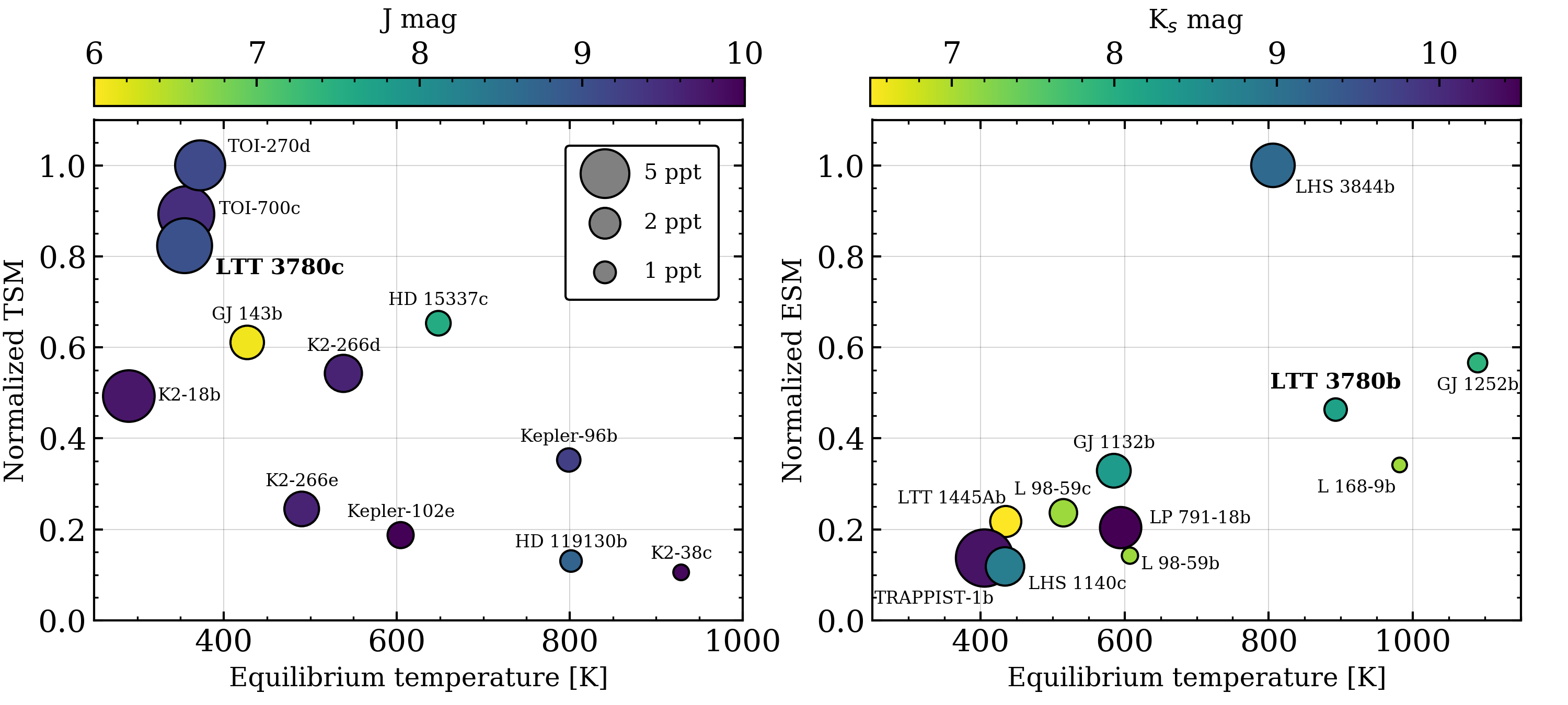
For LTT 3780c, we can also consider the transmission spectroscopy metric (TSM; Kempton et al., 2018) which is proportional to the expected S/N of transmission features in a cloud-free atmosphere. Based on the TSM, LTT 3780c is among the best warm mini-Neptunes ($P\in[10,40]$ days, $r_{p}\in[2,3]$ R_⊕) for atmospheric characterization via transmission spectroscopy observations. To date, the best such planets are the TESS-discovered planets TOI-700c (Gilbert et al., 2020; Rodriguez et al., 2020), TOI-270d (Günther et al., 2019), and LTT 3780c, whose TSM values are all within 17% of each other and are at minimum 17% greater than that of the next best potential target: HD 15337c (Dumusque et al., 2019). The TSM values of favorable warm mini-Neptunes are reported in Table 4 and are compared in Figure 8.

Figure 8: Normalized atmospheric characterization metrics (Kempton et al., 2018) versus equilibrium temperature and host star apparent magnitude. Left panel: the transmission spectroscopy metric (TSM) for warm mini-Neptunes around bright host stars ($J<10$) with $P\in[10,40]$ days and $r_{p}\in[2,3]$ R_⊕, including LTT 3780c. Marker colors depict the host star’s $J$-band magnitude. Right panel: the emission spectroscopy metric (ESM) for favorable close-in rocky planets ($r_{p}<1.5$ R_⊕) including LTT 3780b. Marker colors depict the host star’s $K_{s}$-band magnitude. In both panels the marker sizes depict the primary transit depths.

Table 4: Transmission spectroscopy metric values for warm mini-Neptunes

Planet	$P$	$r_{p}$	$m_{p}$	$Z$	$T_{\text{eq}}$	$J$	$T_{\text{eff}}$	$R_{s}$	$M_{s}$	TSM	TSM-	Refs
name	[days]	[R⊕]	[M⊕]	[ppt]	[K]	mag	[K]	[R⊙]	[M⊙]		normalized
TOI-270d	11.38	2.13	5.48	2.6	372	9.099	3386	0.38	0.40	86.8	1.00	1
TOI-700c	16.05	2.63	7.64	3.3	356	9.469	3480	0.42	0.42	77.5	0.89	2,3
LTT 3780c	12.25	2.30	8.59	3.3	353	9.007	3331	0.37	0.40	71.5	0.82	4
HD 15337c	17.17	2.52	8.79	0.6	648	7.553	5125	0.87	0.90	60.6	0.70	5
GJ 143b	35.61	2.61	22.70	1.2	427	6.081	4640	0.70	0.73	53.0	0.61	6
K2-266d	14.70	2.93	8.90	1.5	538	9.611	4285	0.70	0.69	47.1	0.54	7
K2-18b	32.94	2.71	8.63	2.8	290	9.763	3505	0.47	0.50	42.8	0.49	8
Kepler-96b	15.24	2.67	8.46	0.6	798	9.260	5690	1.02	1.00	30.6	0.35	9
K2-266e	19.48	2.73	14.30	1.3	490	9.611	4285	0.70	0.69	21.3	0.24	7
Kepler-102e	16.15	2.22	8.93	0.7	604	9.984	4909	0.76	0.81	16.3	0.19	9
HD 119130b	16.98	2.63	24.50	0.5	801	8.730	5725	1.09	1.00	11.3	0.13	10
K2-38c	10.56	2.42	9.90	0.3	928	9.911	5757	1.38	2.24	9.2	0.11	11

Note. — References: 1) Günther et al. 2019 2) Gilbert et al. 2020 3) Rodriguez et al. 2020 4) this work 5) Dumusque et al. 2019 6) Dragomir et al. 2019 7) Rodriguez et al. 2018 8) Cloutier et al. 2019b 9) Marcy et al. 2014 10) Luque et al. 2019 11) Sinukoff et al. 2016.

The ultra-short period planet LTT 3780b has a zero-albedo equilibrium temperature of $T_{\text{eq},b}=892$ K. The hot dayside of LTT 3780b makes it a very attractive target for atmospheric characterization via emission spectroscopy observations. In particular, eclipse observations can help to discern whether the planet has retained a substantial atmosphere or if its emitting temperature is consistent with that of pure rock. The distinction between a 1 bar atmosphere and a bare rocky surface on LTT 3780b will be accessible with a single JWST/MIRI eclipse observation (Koll et al., 2019).

Similarly to the TSM, the expected S/N of thermal emission signatures at 7.5 $\mu$m is proportional to the emission spectroscopy metric (ESM; Kempton et al., 2018). Computing the ESM for hot planets with likely terrestrial compositions ($r_{p}<1.5$ R_⊕), that are favorable targets for emission spectroscopy measurements, reveals that LTT 3780b is among the best such planets (Table 5, Figure 8). The ESM for LTT 3780b is the third highest among these planets and closely matches that of GJ 1252b (Shporer et al., 2019). Both of these targets have ESM values that are nearly half that of LHS 3844b (Vanderspek et al., 2019), a rocky planet whose thermal phase curve has been characterized by the Spitzer Space Telescope and found to be consistent with a dark basaltic surface that lacks any substantial atmosphere (Kreidberg et al., 2019).

Table 5: Emission spectroscopy metric values for select close-in Earth-sized planets

Planet	$P$	$r_{p}$	$Z$	$T_{\text{eq}}$	$T_{\text{day}}$	$K_{s}$	$T_{\text{eff}}$	$R_{s}$	$M_{s}$	ESM	ESM-	Refs
name	[days]	[R⊕]	[ppt]	[K]	[K]	mag	[K]	[R⊙]	[M⊙]		normalized
LHS 3844b	0.46	1.30	4.0	805	886	9.145	3036	0.19	0.15	29.0	1.00	1
GJ 1252b	0.52	1.19	0.8	1089	1198	7.915	3458	0.39	0.38	16.4	0.57	2
LTT 3780b	0.77	1.33	1.1	892	982	8.204	3331	0.37	0.40	13.4	0.46	3
L 168-9b	1.40	1.39	0.5	981	1079	7.082	3800	0.60	0.62	9.9	0.34	4
GJ 1132b	1.63	1.13	2.4	585	643	8.322	3270	0.21	0.18	9.5	0.33	5
L 98-59c	3.69	1.35	1.6	515	566	7.101	3412	0.31	0.31	6.9	0.24	6
LTT 1445Ab	5.36	1.38	2.0	435	478	6.500	3335	0.28	0.26	6.3	0.22	7
LP 791-18b	0.95	1.12	3.6	594	653	10.644	2949	0.17	0.14	5.9	0.20	8
L 98-59b	2.25	0.80	0.6	607	668	7.101	3412	0.31	0.31	4.1	0.14	6
TRAPPIST-1b	1.51	1.09	6.9	405	446	10.300	2559	0.12	0.08	4.0	0.14	9
LHS 1140c	3.78	1.28	3.1	434	477	8.821	3216	0.21	0.18	3.4	0.12	10

Note. — References: 1) Vanderspek et al. 2019 2) Shporer et al. 2019 3) this work 4) Astudillo-Defru et al. 2020 5) Berta-Thompson et al. 2015 6) Kostov et al. 2019 7) Winters et al. 2019 8) Crossfield et al. 2019 9) Gillon et al. 2017 10) Ment et al. 2019

The favorable ESM and TSM values of LTT 3780b and c respectively make them both accessible targets for atmospheric characterization. Together they present a unique opportunity to conduct direct comparative studies of exoplanet atmospheres among planets within the same planetary system which is critical for informing our understanding of the formation and evolution of close-in planets at a range of sizes and equilibrium temperatures.

5.5 An independent analysis of the LTT 3780 system by CARMENES

Following the announcement of the planet candidates TOI-732.01 and 02 in May 2019, multiple PRV instrument teams began working towards the mass characterization of these potential planets. This study has presented the subset of those efforts from HARPS and HARPS-N but we acknowledge that the CARMENES team has also submitted a paper presenting their own RV time series and analysis (Nowak et al., 2020). Although the submissions of these complementary studies were coordinated between the two groups, their respective data, analyses, and writeups were intentionally conducted independently.

6 Summary

In this study, we present the LTT 3780 multi-transiting system from the TESS mission. The newly discovered planets LTT 3780b and c are confirmed with intensive follow-up observations that includes ground-based transit photometry, reconnaissance spectroscopy, high-resolution imaging, and 63 precise RV measurements from HARPS and HARPS-N. Our main findings are summarized below.

• LTT 3780 is a bright ($V=13.07$, $K_{s}=8.204$) mid-M dwarf with $M_{s}=0.401\pm 0.012$ M_⊙ and $R_{s}=0.374\pm 0.011$ R_⊙, located at 22 pc.

• LTT 3780b is a hot rocky exoplanet with $P_{b}=0.77$ days, $r_{p,b}=1.33\pm 0.07$ R_⊕, and $m_{p,b}=2.62^{+0.48}_{-0.46}$ M_⊕, making its bulk composition consistent with that of the Earth.

• LTT 3780c is a warm mini-Neptune with $P_{c}=12.25$ days, $r_{p,c}=2.30\pm 0.16$ R_⊕, and $m_{p,c}=8.6^{+1.6}_{-1.3}$ M_⊕. Its bulk composition is inconsistent with being Earth-like and requires a significant amount of volatile material or H/He gas to explain its mass and radius.

• The two planets span the radius valley around low mass stars which enables the comparison of their planetary parameters to predictions from models of the emergence of the radius valley. Both planets’ physical and orbital properties are shown to be consistent with predictions of atmospheric escape from photoevaporation and from core-powered mass loss.

• The brightness and small size of LTT 3780 make the planets LTT 3780b and c accessible targets for atmospheric characterization of a hot rocky planet and a warm mini-Neptune via emission and transmission spectroscopy observations respectively.

Table 6: Point estimates of the LTT 3780 planetary system model parameters

Parameter	Fiducial Model Values	EXOFASTv2 Model Values
TESS light curve parameters
Baseline flux, $f_{0}$	$1.000072\pm 0.000070$	$1.000043\pm 0.000038$
$\ln{\omega_{0}}$	$1.64\pm 1.15$	-
$\ln{S_{0}\omega_{0}^{4}}$	$3.62^{+0.40}_{-0.39}$	-
$\ln{s_{\text{TESS}}^{2}}$	$1.21\pm 0.01$	-
TESS limb darkening coefficient, $u_{1}$	$0.28^{+0.33}_{-0.20}$	$0.30^{+0.07}_{-0.05}$
TESS limb darkening coefficient, $u_{2}$	$0.16^{+0.37}_{-0.28}$	$0.32^{+0.07}_{-0.06}$
Dilution	-	$0.023^{+0.047}_{-0.048}$
RV parameters
$\ln{\lambda/\text{day}}$	$4.5^{+1.0}_{-0.4}$	-
$\ln{\Gamma}$	$-0.1^{+1.3}_{-1.2}$	-
$\ln{P_{\text{GP}}/\text{day}}$	$4.64^{+0.14}_{-0.16}$	-
$\ln{a_{\text{HARPS}}/\text{m/s}}$	$0.52^{+0.69}_{-0.62}$	-
$\ln{a_{\text{HARPS-N}}/\text{m/s}}$	$1.25^{+0.70}_{-0.74}$	-
Jitter, $s_{\text{HARPS}}$ [m s-1]	$0.11^{+0.48}_{-0.09}$	$1.41^{+0.70}_{-0.80}$
Jitter, $s_{\text{HARPS-N}}$ [m s-1]	$1.24^{+0.36}_{-0.46}$	$3.54^{+0.99}_{-0.75}$
Systemic velocity, $\gamma_{\text{HARPS}}$ [m s-1]	$195.5^{+1.4}_{-1.5}$	$195.4^{+0.5}_{-0.5}$
Systemic velocity, $\gamma_{\text{HARPS-N}}$ [m s-1]	$196.8^{+4.6}_{-3.6}$	$194.3^{+1.0}_{-1.0}$
LTT 3780b (TOI-732.01) parameters
Log orbital period, $\ln{P_{b}}$	$-0.26338\pm 0.00007$	-
Orbital period, $P_{b}$ [days]	$0.768448^{+0.000055}_{-0.000053}$	$0.7683881^{+0.0000084}_{-0.0000083}$
Time of mid-transit, $T_{0,b}$ [BJD - 2,457,000]	$1543.9115\pm 0.0011$	$1543.91199^{+0.00059}_{-0.00051}$
Transit duration $D_{b}$ [hrs]	$0.805^{+0.049}_{-0.072}$	$0.786^{+0.024}_{-0.020}$
Transit depth, $Z_{b}$ [ppt]	$1.087^{+0.098}_{-0.103}$	$1.076^{+0.093}_{-0.089}$
Scaled semimajor axis, $a_{b}/R_{s}$	$7.03^{+0.23}_{-0.21}$	$7.05^{+0.24}_{-0.22}$
Planet-to-star radius ratio, $r_{p,b}/R_{s}$	$0.0330^{+0.0014}_{-0.0016}$	$0.0328^{+0.0014}_{-0.0014}$
Impact parameter, $b_{b}$	$0.35^{+0.20}_{-0.23}$	$0.43^{+0.08}_{-0.12}$
Inclination, $i_{b}$ [deg]	$87.1^{+1.8}_{-1.7}$	$86.5^{+1.0}_{-0.7}$
Eccentricity, $e_{b}$	0 (fixed)	0 (fixed)
Planet radius, $r_{p,b}$ [R⊕]	$1.332^{+0.072}_{-0.075}$	$1.321^{+0.074}_{-0.073}$
Log RV semi-amplitude, $\ln{K_{b}}$	$1.23^{+0.14}_{-0.17}$	$1.26^{+0.14}_{-0.17}$
RV semi-amplitude, $K_{b}$ [m s-1]	$3.41^{+0.63}_{-0.63}$	$3.54^{+0.54}_{-0.55}$
Planet mass, $m_{p,b}$ [M⊕]	$2.62^{+0.48}_{-0.46}$	$2.77^{+0.43}_{-0.43}$
Bulk density, $\rho_{b}$ [g cm-3]	$6.1^{+1.8}_{-1.5}$	$6.5^{+1.7}_{-1.4}$
Surface gravity, $g_{b}$ [m s-2]	$14.4^{+3.7}_{-3.3}$	$15.5^{+3.6}_{-3.4}$
Escape velocity, $v_{\text{esc},b}$ [km s-1]	$15.7^{+1.5}_{-1.5}$	$16.2^{+1.3}_{-1.4}$
Semimajor axis, $a_{b}$ [AU]	$0.01211^{+0.00012}_{-0.00012}$	$0.01212^{+0.00012}_{-0.00012}$
Insolation, $F_{b}$ [F⊕]	$106^{+22}_{-19}$	$106^{+23}_{-19}$
Equilibrium temperature, $T_{\text{eq},b}$ [K]
Bond albedo = 0.0	$892\pm 44$	$892\pm 44$
Bond albedo = 0.3	$816\pm 40$	$816\pm 40$
LTT 3780c (TOI-732.02) parameters
Log orbital period, $\ln{P_{c}}$	$2.50582\pm 0.00023$	-
Orbital period, $P_{c}$ [days]	$12.2519^{+0.0028}_{-0.0030}$	$12.252048^{+0.000060}_{-0.000059}$
Time of mid-transit, $T_{0,c}$ [BJD - 2,457,000]	$1546.8484\pm 0.0014$	$1546.8481^{+0.0011}_{-0.0012}$
Transit duration $D_{c}$ [hrs]	$1.392^{+0.050}_{-0.049}$	$1.404^{+0.048}_{-0.046}$
Transit depth, $Z_{c}$ [ppt]	$3.24^{+0.41}_{-0.37}$	$3.13^{+0.28}_{-0.28}$
Scaled semimajor axis, $a_{c}/R_{s}$	$44.6^{+1.5}_{-1.3}$	$44.7^{+1.5}_{-1.4}$
Planet-to-star radius ratio, $r_{p,c}/R_{s}$	$0.0570^{+0.0035}_{-0.0033}$	$0.0560^{+0.0024}_{-0.0025}$
Impact parameter, $b_{c}$	$0.65^{+0.15}_{-0.36}$	$0.71^{+0.08}_{-0.15}$
Inclination, $i_{c}$ [deg]	$89.18^{+0.47}_{-0.22}$	$88.95^{+0.10}_{-0.09}$
$e_{c}\cos{\omega_{c}}$	-	$-0.05^{+0.07}_{-0.08}$
$e_{c}\sin{\omega_{c}}$	-	$0.15^{+0.15}_{-0.13}$
$\sqrt{e_{c}}\cos{\omega_{c}}$	$0.13^{+0.12}_{-0.15}$	-
$\sqrt{e_{c}}\sin{\omega_{c}}$	$0.07^{+0.17}_{-0.19}$	-
Eccentricity, $e_{c}$	$0.06^{+0.15}_{-0.14}$	$0.18^{+0.14}_{-0.11}$
Argument of periastron, $\omega_{c}$ [deg]	$124^{+87}_{-147}$	$111^{+39}_{-27}$
Planet radius, $r_{p,c}$ [R⊕]	$2.30^{+0.16}_{-0.15}$	$2.25^{+0.13}_{-0.13}$
Log RV semi-amplitude, $\ln{K_{c}}$	$1.49^{+0.17}_{-0.17}$	$1.60^{+0.13}_{-0.15}$
RV semi-amplitude, $K_{c}$ [m s-1]	$4.44^{+0.82}_{-0.68}$	$4.94^{+0.68}_{-0.67}$
Planet mass, $m_{p,c}$ [M⊕]	$8.6^{+1.6}_{-1.3}$	$9.5^{+1.3}_{-1.3}$
Bulk density, $\rho_{c}$ [g cm-3]	$3.9^{+1.0}_{-0.9}$	$4.6^{+1.1}_{-0.9}$
Surface gravity, $g_{c}$ [m s-2]	$16.0^{+3.7}_{-3.3}$	$18.3^{+3.5}_{-3.1}$
Escape velocity, $v_{\text{esc},c}$ [km s-1]	$21.7^{+2.1}_{-2.0}$	$23.0^{+1.7}_{-1.7}$
Semimajor axis, $a_{c}$ [AU]	$0.07673^{+0.00075}_{-0.00077}$	$0.07678^{+0.00076}_{-0.00077}$
Insolation, $F_{c}$ [F⊕]	$2.63^{+0.56}_{-0.48}$	$2.63^{+0.56}_{-0.48}$
Equilibrium temperature, $T_{\text{eq},c}$ [K]
Bond albedo = 0.0	$353\pm 18$	$354\pm 18$
Bond albedo = 0.3	$323\pm 16$	$324\pm 16$

Appendix A Limits on the planet masses for consistency with models of photoevaporation

Here we present the formalism used to estimate mass limits on planets spanning the radius valley within a multi-transiting system under the photoevaporation model (Owen & Campos Estrada, 2020). This model is adopted from Owen & Wu (2017) in which a population of non-rocky planets is formed with a distribution of Earth-like core masses plus H/He envelopes. The energy-limited atmospheric mass loss rate due to XUV heating by the host star, and subsequent thermal escape, is $\dot{M}_{\text{atm}}=\eta_{p}\pi r_{\text{core}}^{3}L_{\text{XUV}}/4\pi a^{2}Gm_{\text{core}}$ where $\eta_{p},r_{\text{core}},a,m_{\text{core}}$ are the planet’s mass-loss efficiency, core radius, orbital separation, and core mass respectively, $L_{\text{XUV}}$ is the XUV luminosity of the host star and $G$ is the gravitational constant. By writing the atmospheric mass as the product of the planet mass and envelope mass fraction ($M_{\text{atm}}=m_{p}\>X_{2}$), the mass loss timescale under photoevaporation ($t_{\text{loss}}=M_{\text{atm}}/\dot{M}_{\text{atm}}$) scales as

$$t_{\text{loss}} \propto\frac{m_{p}^{2}\>a^{2}\>X_{2}}{\eta_{p}\>r_{\text{core}}^{3}\>L_{\text{XUV}}}$$

$$\propto\frac{m_{p}^{3}\>a^{2}\>X_{2}}{r_{\text{core}}^{4}\>L_{\text{XUV}}}$$ (A1)

where we have adopted $\eta_{p}\propto v_{\text{esc}}^{-2}\propto m_{\text{core}}^{-1}r_{\text{core}}$ (Owen & Wu, 2017) and set $m_{\text{core}}=m_{p}$ by assuming that the planet masses are dominated by their rocky core masses. In this simple picture, Owen & Campos Estrada (2020) set Equation A1 to the maximum mass loss timescale for a rocky planet below the valley which is assumed to have just lost the entirety of its initial H/He envelope. In order to form the radius valley, this timescale must be less than the maximum timescale for the gaseous (i.e. non-rocky) planet to have retained its initial H/He envelope with an atmospheric mass fraction of $X_{2}$. This criterion places the following constrains on the rocky and gaseous planet parameters according to

$$\frac{t_{\text{loss,gas}}}{t_{\text{loss,rock}}}\geq 1,$$

$$\left(\frac{m_{p,\text{gas}}}{m_{p,\text{rock}}}\right)\left(\frac{a_{\text{gas}}}{a_{\text{rock}}}\right)^{2/3}\left(\frac{r_{\text{core,gas}}}{r_{\text{core,rock}}}\right)^{-4/3}\geq 1.$$ (A2)

The power of comparing planets within the same planetary system is evidenced in Equation A2 in which the unknown quantity $L_{\text{XUV}}$ is scaled out of the expression.

In the photoevaporation model, the stripped rocky planet has been reduced to its Earth-like core such that the core radius is equivalent to the planet’s radius; $r_{\text{core,rock}}=r_{p,\text{rock}}$. Noting that $r_{\text{core}}\propto m_{\text{core}}^{0.27}$ for Earth-like bodies (Zeng et al., 2016), we write $r_{\text{core,gas}}=m_{p,gas}^{0.27}$ where the input radius and mass are each given in units of the Earth. It follows from Equation A2 that the minimum mass of the gaseous planet under the photoevaporation model is

$$\frac{m_{p,\text{gas}}}{\text{M}_{\oplus}}\geq\left[\left(\frac{m_{p,\text{rock}}}{\text{M}_{\oplus}}\right)\left(\frac{a_{\text{rock}}}{a_{\text{gas}}}\right)^{2/3}\>\left(\frac{r_{p,\text{rock}}}{\text{R}_{\oplus}}\right)^{-4/3}\right]^{1.56}.$$ (A3)

The inequality in Equation A3 must be satisfied for the planetary parameters to be consistent with the photoevaporation model. Similarly,

$$\frac{m_{p,\text{rock}}}{\text{M}_{\oplus}}\leq\left(\frac{m_{p,\text{gas}}}{\text{M}_{\oplus}}\right)^{0.64}\left(\frac{a_{\text{gas}}}{a_{\text{rock}}}\right)^{2/3}\>\left(\frac{r_{p,\text{rock}}}{\text{R}_{\oplus}}\right)^{4/3}$$ (A4)

represents the maximum mass of the rocky planet for the system to be consistent with the photoevaporation model.

A few notable caveats exist with this simplified model (Owen & Campos Estrada, 2020). Specifically, these calculations assumed that the envelope mass fraction $X_{2}$ for which the mass loss timescales are maximized, is independent of the planet properties. Furthermore, individual gaseous planets may have envelope mass fractions that are greater than that which is required to maximize $t_{\text{loss,gas}}$. Lastly, this simplified model ignores the contraction of the H/He envelope over time. This poses a critical limitation as gaseous envelopes are likely to have been more extended at early times when photoevaporation was actively ongoing, compared to their present day values.

These issues are alleviated by the EvapMass software Owen & Campos Estrada (2020) which calculates the value of $X_{2}$ that maximizes the mass loss timescale and self-consistently models the gaseous envelope structure from the typical Kelvin-Helmholtz time of the gaseous envelope $(\tau_{\text{KH}}\sim 100$ Myrs) to the present. However, attempting these numerical calculations on the LTT 3780 system resulted in a failure to solve for a lower limit on the LTT 3780c core mass. By default, EvapMass only considers $m_{\text{core,gas}}\geq 0.1$ M_⊕, which is itself a very weak constraint, such that the EvapMass calculation does not provide any new insight into the minimum mass of LTT 3780c.

Appendix B Limits on the planet masses for consistency with models of core-powered mass loss

Here we derive the constraints on the planet masses in order to be consistent with the core-powered mass loss model for sculpting the radius valley. Analogously to the formalism presented in Appendix A, we compare the timescales for core-powered mass loss of planets spanning the radius valley and within the same multi-transiting system.

Core-powered mass loss is another mechanism for driving thermal escape of a planet’s atmosphere due to the planetary core’s own cooling luminosity (Ginzburg et al., 2018; Gupta & Schlichting, 2019). Similarly to the initial conditions assumed in the photoevaporation model, here a population of non-rocky planets is formed with a distribution of Earth-like core masses plus H/He envelopes. Their atmospheres are described by a lower convective region which is terminated at the radius of the radiative-convective boundary (RCB), above which the atmosphere becomes isothermal and heat is transported radiatively to the planet’s Bondi radius. The Bondi radius is set by equating the planet’s escape velocity to its thermal sound speed and is $R_{\text{B}}=Gm_{\text{core}}/c_{s}^{2}$, where $G$ is the gravitational constant, $m_{\text{core}}$ is the core mass, and the thermal sound speed is $c_{s}=\sqrt{k_{B}T_{\text{eq}}/\mu}$, where $k_{B}$ is the Boltzmann constant, $T_{\text{eq}}$ is the equilibrium temperature, and $\mu$ is the atmospheric mean molecular weight, assumed to be 2 amu for H₂. The Bondi-limited regime represents the physical limit of the atmospheric mass loss rate and is dictated by the gas thermal velocity at $R_{\text{B}}$.

The corresponding Bondi-limited mass loss rate is $\dot{M}_{\text{atm}}=4\pi R_{\text{B}}^{2}c_{s}\rho_{\text{RCB}}\exp{(-Gm_{\text{core}}/c_{s}^{2}R_{\text{RCB}})}$ where $\rho_{\text{RCB}}$ is the atmospheric density at the RCB whose radius is $R_{\text{RCB}}$. The majority of the atmosphere’s mass lies within its convective zone such that integrating an adiabatic gas density profile over the convective zone returns the approximate atmospheric mass

$$M_{\text{atm}}\approx 4\pi R_{\text{RCB}}^{3}\rho_{\text{RCB}}\left(\frac{\gamma-1}{\gamma}\frac{R_{\text{B}}}{R_{\text{RCB}}}\right)^{1/(\gamma-1)}$$ (B1)

where $\gamma$ is the adiabatic index which is fixed to $4/3$ (Ginzburg et al., 2016). The resulting mass loss timescale ($t_{\text{loss}}=M_{\text{atm}}/\dot{M}_{\text{atm}}$) scales as

$$t_{\text{loss}} \propto\frac{R_{\text{B}}}{c_{s}}\>\exp{\left(\frac{Gm_{\text{core}}}{c_{s}^{2}R_{\text{RCB}}}\right)},$$

$$\propto\frac{m_{p}}{T_{\text{eq}}^{3/2}}\>\exp{\left(\frac{c^{\prime}m_{p}}{T_{\text{eq}}r_{p}}\right)},$$ (B2)

where the constant $c^{\prime}=G\mu/k_{B}\sim 10^{4}$ R_⊕ K M_⊕^-1, the planet’s envelope mass fraction is assumed to be small such that $m_{\text{core}}\approx m_{p}$, and the $R_{\text{RCB}}$ is treated as the planet’s effective radius; $R_{\text{RCB}}\approx r_{p}$.

Analogously to the photoevaporation scenario, for the planetary parameters within a multi-transiting system and spanning the radius valley to be consistent with the core-powered mass loss scenario, we require that the mass loss timescale of the gaseous (i.e. non-rocky) planet exceeds that of the rocky planet. This leads to the following condition:

$$\frac{t_{\text{loss,gas}}}{t_{\text{loss,rock}}} \geq 1,$$

$$\left(\frac{m_{p,\text{gas}}}{m_{p,\text{rock}}}\right)\left(\frac{T_{\text{eq,gas}}}{T_{\text{eq,rock}}}\right)^{-3/2}$$

$$\exp{\left[c^{\prime}\left(\frac{m_{p,\text{gas}}}{T_{\text{eq,gas}}\>r_{p,\text{gas}}}-\frac{m_{p,\text{rock}}}{T_{\text{eq,rock}}\>r_{p,\text{rock}}}\right)\right]} \geq 1.$$ (B4)

The appearance of the planet masses as both linear factors and in the exponential function means that Equation B4 belongs to the class of Lambert $W$ functions of the form $f(m)\propto m\text{e}^{m}$. Such functions do not have analytical solutions but the limiting planet masses under the core-powered mass loss model can be solved for numerically.

References

- Anglada-Escudé & Butler (2012) Anglada-Escudé, G., & Butler, R. P. 2012, ApJS, 200, 15
- Astropy Collaboration et al. (2013) Astropy Collaboration, Robitaille, T. P., Tollerud, E. J., et al. 2013, A&A, 558, A33
- Astropy Collaboration et al. (2018) Astropy Collaboration, Price-Whelan, A. M., Sipőcz, B. M., et al. 2018, AJ, 156, 123
- Astudillo-Defru et al. (2017) Astudillo-Defru, N., Delfosse, X., Bonfils, X., et al. 2017, A&A, 600, A13
- Astudillo-Defru et al. (2020) Astudillo-Defru, N., Cloutier, R., Wang, S. X., et al. 2020, arXiv e-prints, arXiv:2001.09175
- Ballard & Johnson (2016) Ballard, S., & Johnson, J. A. 2016, ApJ, 816, 66
- Barkaoui et al. (2019) Barkaoui, K., Burdanov, A., Hellier, C., et al. 2019, AJ, 157, 43
- Batalha et al. (2017) Batalha, N. E., Mandell, A., Pontoppidan, K., et al. 2017, PASP, 129, 064501
- Benedict et al. (2016) Benedict, G. F., Henry, T. J., Franz, O. G., et al. 2016, AJ, 152, 141
- Berta-Thompson et al. (2015) Berta-Thompson, Z. K., Irwin, J., Charbonneau, D., et al. 2015, Nature, 527, 204
- Bonfils et al. (2018) Bonfils, X., Almenara, J.-M., Cloutier, R., et al. 2018, A&A, 618, A142
- Brown et al. (2013) Brown, T. M., Baliber, N., Bianco, F. B., et al. 2013, Publications of the Astronomical Society of the Pacific, 125, 1031
- Bryson et al. (2010) Bryson, S. T., Jenkins, J. M., Klaus, T. C., et al. 2010, Society of Photo-Optical Instrumentation Engineers (SPIE) Conference Series, Vol. 7740, Selecting pixels for Kepler downlink, 77401D
- Chen & Rogers (2016) Chen, H., & Rogers, L. A. 2016, ApJ, 831, 180
- Chen & Kipping (2017) Chen, J., & Kipping, D. 2017, ApJ, 834, 17
- Ciardi et al. (2015) Ciardi, D. R., Beichman, C. A., Horch, E. P., & Howell, S. B. 2015, ApJ, 805, 16
- Claret & Bloemen (2011) Claret, A., & Bloemen, S. 2011, A&A, 529, A75
- Cloutier et al. (2014) Cloutier, R., Currie, T., Rieke, G. H., et al. 2014, ApJ, 796, 127
- Cloutier & Menou (2020) Cloutier, R., & Menou, K. 2020, AJ, 159, 211
- Cloutier et al. (2019a) Cloutier, R., Astudillo-Defru, N., Bonfils, X., et al. 2019a, A&A, 629, A111
- Cloutier et al. (2019b) Cloutier, R., Astudillo-Defru, N., Doyon, R., et al. 2019b, A&A, 621, A49
- Collins et al. (2017) Collins, K. A., Kielkopf, J. F., Stassun, K. G., & Hessman, F. V. 2017, AJ, 153, 77
- Crossfield & Kreidberg (2017) Crossfield, I. J. M., & Kreidberg, L. 2017, AJ, 154, 261
- Crossfield et al. (2015) Crossfield, I. J. M., Petigura, E., Schlieder, J. E., et al. 2015, ApJ, 804, 10
- Crossfield et al. (2019) Crossfield, I. J. M., Waalkes, W., Newton, E. R., et al. 2019, ApJ, 883, L16
- Cutri & et al. (2014) Cutri, R. M., & et al. 2014, VizieR Online Data Catalog, II/328
- Cutri et al. (2003) Cutri, R. M., Skrutskie, M. F., van Dyk, S., et al. 2003, 2MASS All Sky Catalog of point sources.
- Damasso et al. (2018) Damasso, M., Bonomo, A. S., Astudillo-Defru, N., et al. 2018, A&A, 615, A69
- Dittmann et al. (2017) Dittmann, J. A., Irwin, J. M., Charbonneau, D., et al. 2017, Nature, 544, 333
- Dotter (2016) Dotter, A. 2016, ApJS, 222, 8
- Dragomir et al. (2019) Dragomir, D., Teske, J., Günther, M. N., et al. 2019, ApJ, 875, L7
- Dressing & Charbonneau (2015) Dressing, C. D., & Charbonneau, D. 2015, ApJ, 807, 45
- Dumusque et al. (2019) Dumusque, X., Turner, O., Dorn, C., et al. 2019, A&A, 627, A43
- Eastman et al. (2013) Eastman, J., Gaudi, B. S., & Agol, E. 2013, PASP, 125, 83
- Eastman et al. (2019) Eastman, J. D., Rodriguez, J. E., Agol, E., et al. 2019, arXiv e-prints, arXiv:1907.09480
- Evans et al. (2018) Evans, D. W., Riello, M., De Angeli, F., et al. 2018, A&A, 616, A4
- Foreman-Mackey et al. (2017) Foreman-Mackey, D., Agol, E., Ambikasaran, S., & Angus, R. 2017, AJ, 154, 220
- Foreman-Mackey et al. (2019) Foreman-Mackey, D., Barentsen, G., & Barclay, T. 2019, dfm/exoplanet: exoplanet v0.1.6, doi:10.5281/zenodo.2651251
- Foreman-Mackey et al. (2013) Foreman-Mackey, D., Hogg, D. W., Lang, D., & Goodman, J. 2013, PASP, 125, 306
- Fortney et al. (2013) Fortney, J. J., Mordasini, C., Nettelmann, N., et al. 2013, ApJ, 775, 80
- Fu et al. (2017) Fu, G., Deming, D., Knutson, H., et al. 2017, ApJ, 847, L22
- Fulton et al. (2017) Fulton, B. J., Petigura, E. A., Howard, A. W., et al. 2017, AJ, 154, 109
- Gaia Collaboration et al. (2018) Gaia Collaboration, Brown, A. G. A., Vallenari, A., et al. 2018, A&A, 616, A1
- Gilbert et al. (2020) Gilbert, E. A., Barclay, T., Schlieder, J. E., et al. 2020, arXiv e-prints, arXiv:2001.00952
- Gillon et al. (2013) Gillon, M., Jehin, E., Fumel, A., Magain, P., & Queloz, D. 2013, in European Physical Journal Web of Conferences, Vol. 47, European Physical Journal Web of Conferences, 03001
- Gillon et al. (2017) Gillon, M., Triaud, A. H. M. J., Demory, B.-O., et al. 2017, Nature, 542, 456
- Ginzburg et al. (2016) Ginzburg, S., Schlichting, H. E., & Sari, R. 2016, ApJ, 825, 29
- Ginzburg et al. (2018) —. 2018, MNRAS, 476, 759
- Goldreich & Soter (1966) Goldreich, P., & Soter, S. 1966, Icarus, 5, 375
- Günther et al. (2019) Günther, M. N., Pozuelos, F. J., Dittmann, J. A., et al. 2019, Nature Astronomy, 3, 1099
- Gupta & Schlichting (2019) Gupta, A., & Schlichting, H. E. 2019, MNRAS, 487, 24
- Gupta & Schlichting (2020) —. 2020, MNRAS, arXiv:1907.03732
- Hadden (2019) Hadden, S. 2019, shadden/TTV2Fast2Furious: First release of TTV2Fast2Furious, doi:10.5281/zenodo.3356829
- Haisch et al. (2001) Haisch, Karl E., J., Lada, E. A., & Lada, C. J. 2001, AJ, 121, 2065
- Hardegree-Ullman et al. (2019) Hardegree-Ullman, K. K., Cushing, M. C., Muirhead, P. S., & Christiansen, J. L. 2019, AJ, 158, 75
- Hardegree-Ullman et al. (2020) Hardegree-Ullman, K. K., Zink, J. K., Christiansen, J. L., et al. 2020, arXiv e-prints, arXiv:2001.11511
- Hodapp et al. (2003) Hodapp, K. W., Jensen, J. B., Irwin, E. M., et al. 2003, PASP, 115, 1388
- Jehin et al. (2011) Jehin, E., Gillon, M., Queloz, D., et al. 2011, The Messenger, 145, 2
- Jenkins (2002) Jenkins, J. M. 2002, ApJ, 575, 493
- Jenkins et al. (2010) Jenkins, J. M., Chandrasekaran, H., McCauliff, S. D., et al. 2010, in SPIE, Vol. 7740, Software and Cyberinfrastructure for Astronomy, 77400D
- Jenkins et al. (2016) Jenkins, J. M., Twicken, J. D., McCauliff, S., et al. 2016, in SPIE, Vol. 9913, Software and Cyberinfrastructure for Astronomy IV, 99133E
- Jensen (2013) Jensen, E. 2013, Tapir: A web interface for transit/eclipse observability, ascl:1306.007
- Jin & Mordasini (2018) Jin, S., & Mordasini, C. 2018, ApJ, 853, 163
- Jin et al. (2014) Jin, S., Mordasini, C., Parmentier, V., et al. 2014, ApJ, 795, 65
- Kempton et al. (2018) Kempton, E. M. R., Bean, J. L., Louie, D. R., et al. 2018, Publications of the Astronomical Society of the Pacific, 130, 114401
- Kipping (2013) Kipping, D. M. 2013, MNRAS, 434, L51
- Koll et al. (2019) Koll, D. D. B., Malik, M., Mansfield, M., et al. 2019, ApJ, 886, 140
- Kostov et al. (2019) Kostov, V. B., Schlieder, J. E., Barclay, T., et al. 2019, AJ, 158, 32
- Kreidberg (2015) Kreidberg, L. 2015, PASP, 127, 1161
- Kreidberg et al. (2015) Kreidberg, L., Line, M. R., Bean, J. L., et al. 2015, ApJ, 814, 66
- Kreidberg et al. (2019) Kreidberg, L., Koll, D. D. B., Morley, C., et al. 2019, Nature, 573, 87
- Lee & Chiang (2016) Lee, E. J., & Chiang, E. 2016, ApJ, 817, 90
- Lee et al. (2014) Lee, E. J., Chiang, E., & Ormel, C. W. 2014, ApJ, 797, 95
- Li et al. (2019) Li, J., Tenenbaum, P., Twicken, J. D., et al. 2019, Publications of the Astronomical Society of the Pacific, 131, 024506
- Lindegren et al. (2018) Lindegren, L., Hernández, J., Bombrun, A., et al. 2018, A&A, 616, A2
- Lopez & Fortney (2014) Lopez, E. D., & Fortney, J. J. 2014, ApJ, 792, 1
- Lopez & Rice (2018) Lopez, E. D., & Rice, K. 2018, MNRAS, 479, 5303
- Lovis & Pepe (2007) Lovis, C., & Pepe, F. 2007, A&A, 468, 1115
- Luger et al. (2019) Luger, R., Agol, E., Foreman-Mackey, D., et al. 2019, AJ, 157, 64
- Luque et al. (2019) Luque, R., Nowak, G., Pallé, E., et al. 2019, A&A, 623, A114
- Luyten (1979) Luyten, W. J. 1979, LHS catalogue. A catalogue of stars with proper motions exceeding 0”5 annually
- Mandel & Agol (2002) Mandel, K., & Agol, E. 2002, ApJL, 580, L171
- Mann et al. (2015) Mann, A. W., Feiden, G. A., Gaidos, E., Boyajian, T., & von Braun, K. 2015, ApJ, 804, 64
- Marcy et al. (2014) Marcy, G. W., Isaacson, H., Howard, A. W., et al. 2014, ApJs, 210, 20
- Martinez et al. (2019) Martinez, C. F., Cunha, K., Ghezzi, L., & Smith, V. V. 2019, ApJ, 875, 29
- Mayo et al. (2018) Mayo, A. W., Vanderburg, A., Latham, D. W., et al. 2018, AJ, 155, 136
- Mayor et al. (2003) Mayor, M., Pepe, F., Queloz, D., et al. 2003, The Messenger, 114, 20
- McCully et al. (2018) McCully, C., Volgenau, N. H., Harbeck, D.-R., et al. 2018, in Society of Photo-Optical Instrumentation Engineers (SPIE) Conference Series, Vol. 10707, Proc. SPIE, 107070K
- Ment et al. (2019) Ment, K., Dittmann, J. A., Astudillo-Defru, N., et al. 2019, AJ, 157, 32
- Montet et al. (2015) Montet, B. T., Morton, T. D., Foreman-Mackey, D., et al. 2015, ApJ, 809, 25
- Mortier et al. (2015) Mortier, A., Faria, J. P., Correia, C. M., Santerne, A., & Santos, N. C. 2015, A&A, 573, A101
- Muirhead et al. (2018) Muirhead, P. S., Dressing, C. D., Mann, A. W., et al. 2018, AJ, 155, 180
- Nowak et al. (2020) Nowak, G., Luque, R., Parviainen, H., et al. 2020, arXiv e-prints, arXiv:2003.01140
- Owen & Campos Estrada (2020) Owen, J. E., & Campos Estrada, B. 2020, MNRAS, 491, 5287
- Owen & Wu (2013) Owen, J. E., & Wu, Y. 2013, ApJ, 775, 105
- Owen & Wu (2017) —. 2017, ApJ, 847, 29
- Rackham et al. (2018) Rackham, B. V., Apai, D., & Giampapa, M. S. 2018, ApJ, 853, 122
- Reid et al. (2002) Reid, I. N., Kilkenny, D., & Cruz, K. L. 2002, AJ, 123, 2822
- Ricker et al. (2015) Ricker, G. R., Winn, J. N., Vanderspek, R., et al. 2015, Journal of Astronomical Telescopes, Instruments, and Systems, 1, 014003
- Rodriguez et al. (2018) Rodriguez, J. E., Becker, J. C., Eastman, J. D., et al. 2018, AJ, 156, 245
- Rodriguez et al. (2020) Rodriguez, J. E., Vanderburg, A., Zieba, S., et al. 2020, arXiv e-prints, arXiv:2001.00954
- Salvatier et al. (2016) Salvatier, J., Wiecki, T. V., & Fonnesbeck, C. 2016, PeerJ Computer Science, 2, e55
- Scholz et al. (2005) Scholz, R. D., Meusinger, H., & Jahreiß, H. 2005, A&A, 442, 211
- Shporer et al. (2019) Shporer, A., Collins, K. A., Astudillo-Defru, N., et al. 2019, arXiv e-prints, arXiv:1912.05556
- Sinukoff et al. (2016) Sinukoff, E., Howard, A. W., Petigura, E. A., et al. 2016, ApJ, 827, 78
- Smith et al. (2012) Smith, J. C., Stumpe, M. C., Van Cleve, J. E., et al. 2012, PASP, 124, 1000
- Stassun et al. (2017) Stassun, K. G., Oelkers, R. J., Pepper, J., et al. 2017, ArXiv e-prints, arXiv:1706.00495
- Stassun et al. (2019) Stassun, K. G., Oelkers, R. J., Paegert, M., et al. 2019, AJ, 158, 138
- Stevenson (2016) Stevenson, K. B. 2016, ApJ, 817, L16
- Stumpe et al. (2014) Stumpe, M. C., Smith, J. C., Catanzarite, J. H., et al. 2014, PASP, 126, 100
- Stumpe et al. (2012) Stumpe, M. C., Smith, J. C., Van Cleve, J. E., et al. 2012, PASP, 124, 985
- Tokovinin (2018) Tokovinin, A. 2018, PASP, 130, 035002
- Twicken et al. (2018) Twicken, J. D., Catanzarite, J. H., Clarke, B. D., et al. 2018, Publications of the Astronomical Society of the Pacific, 130, 064502
- Van Eylen et al. (2018) Van Eylen, V., Agentoft, C., Lundkvist, M. S., et al. 2018, MNRAS, 479, 4786
- Vanderspek et al. (2019) Vanderspek, R., Huang, C. X., Vanderburg, A., et al. 2019, ApJ, 871, L24
- Virtanen et al. (2020) Virtanen, P., Gommers, R., Oliphant, T. E., et al. 2020, Nature Methods, doi:https://doi.org/10.1038/s41592-019-0686-2
- Winters et al. (2019) Winters, J. G., Medina, A. A., Irwin, J. M., et al. 2019, AJ, 158, 152
- Wu (2019) Wu, Y. 2019, ApJ, 874, 91
- Zeng & Sasselov (2013) Zeng, L., & Sasselov, D. 2013, PASP, 125, 227
- Zeng et al. (2016) Zeng, L., Sasselov, D. D., & Jacobsen, S. B. 2016, ApJ, 819, 127
- Zeng et al. (2019) Zeng, L., Jacobsen, S. B., Sasselov, D. D., et al. 2019, Proceedings of the National Academy of Science, 116, 9723
- Ziegler et al. (2020) Ziegler, C., Tokovinin, A., Briceño, C., et al. 2020, AJ, 159, 19