Suppression of scalar power on large scales and associated bispectra

Abstract

A sharp cut-off in the primordial scalar power spectrum on large scales has been known to improve the fit to the cosmic microwave background (CMB) data when compared to the more standard, nearly scale invariant power spectra that arise in slow roll inflation. Over the last couple of years, there has been a resurgent interest in arriving at such power spectra in models with kinetically dominated initial conditions for the background scalar field which leads to inflation of specific duration. In an earlier work, we had numerically investigated the characteristics of the scalar bispectrum generated in such models. In this work, we compare the scenario with two other competing scenarios (viz. punctuated inflation and a model due to Starobinsky) which also suppress the scalar power in a roughly similar fashion on large scales. We further consider two other scenarios involving inflation of a finite duration, one wherein the scalar field begins on the inflationary attractor and another wherein the field starts with a smaller velocity and evolves towards the attractor. These scenarios too exhibit a sharp drop in power on large scales if the initial conditions on the perturbations for a range of modes are imposed on super-Hubble scales as in the kinetically dominated model. We compare the performance of all the models against the Planck CMB data at the level of scalar power spectra. The model wherein the background field always remains on the inflationary attractor is interesting for the reason that it permits analytical calculations of the scalar power and bi-spectrum. We also compare the amplitudes and shapes of the scalar non-Gaussianity parameter $f_{{}_{\mathrm{NL}}}$ in all these cases which lead to scalar power spectra of similar form. Interestingly, we find that, in the models wherein the initial conditions on the perturbations are imposed on super-Hubble scales, the consistency relation governing the scalar bispectrum is violated for the large scale modes, whereas the relation is satisfied for all the modes in the other scenarios. These differences in the behavior of the scalar bispectra can conceivably help us observationally discriminate between the various models which lead to scalar power spectra of roughly similar shape.

I Introduction

Ever since the advent of the three-year WMAP data, it has been repeatedly found that a sharp drop in power at large scales roughly corresponding to the Hubble radius today improves the fit to the anisotropies in the cosmic microwave background (CMB) at the low multipoles (for an early analysis, see, for instance, Ref. [1]; for later discussions in this context, see Refs. [2, 3, 4, 5]). A variety of inflationary scenarios have been constructed to generate such a drop in power on large scales (for a short list of possibilities, see Refs. [6, 7, 8, 9, 10, 11, 12, 13, 14, 15, 16, 17, 18, 19, 20]).

One of the scenarios that generates a scalar spectrum with suppressed power on large scales corresponds to a situation wherein the scalar field driving inflation starts rolling down the potential with a high velocity (for the original discussion, see Ref. [7]; for more recent discussions, see Refs. [21, 22, 23, 24, 25]). While the very early kinetically dominated phase does not permit accelerated expansion, the friction arising due to the expansion of the universe slows down the field, initially leading to a brief period of fast roll inflation and eventually to the standard phase of slow roll inflation. If one chooses the beginning of inflation to occur at an appropriately early time, the inflationary power spectra exhibit lower power at suitably large scales, improving the fit to the CMB data at the low multipoles [25]. However, it should be emphasized that, in such scenarios, a range of large scale modes are never inside the Hubble radius and spectra with a suppression of power arise provided the standard Bunch-Davies initial conditions are imposed on super-Hubble scales [7, 25].

A competing inflationary scenario that, in fact, leads to sharper drop in power at the large scales corresponds to a short phase of fast roll sandwiched between two epochs of slow roll inflation. Such scenarios can be further sub-divided into two categories: one wherein inflation is sustained even during the phase of fast roll and another wherein the epoch of fast roll leads to a brief departure from inflation. While the first type of scenario can be achieved in a model originally due to Starobinsky involving a linear potential with an abrupt change in slope [26], the second type of scenario—dubbed punctuated inflation—is known to arise due to inflationary potentials containing a point of inflection [14, 15]. The advantage of such scenarios is that the initial epoch of slow roll inflation permits one to impose the standard Bunch-Davies initial conditions in the sub-Hubble domain for all the modes of cosmological interest.

As we shall see, these alternative scenarios lead to scalar power spectra which have almost the same shape. Moreover, as we shall illustrate, these power spectra also lead to a slightly improved fit to the CMB data than the nearly scale invariant power spectra. One can expect that non-Gaussianities, specifically, the scalar bispectrum, would help us discriminate between these models. In an earlier work, we had numerically computed the scalar bispectrum and the corresponding non-Gaussianity parameter $f_{{}_{\mathrm{NL}}}$ that arise in models with kinetically dominated initial conditions [27]. Interestingly, we had found that, in such a scenario, the contributions due to the boundary terms in the third order action governing the scalar perturbations dominate the contributions due to the bulk terms. In this work, we shall discuss in detail the various contributions to the scalar bispectrum that arise as well as the numerical procedure that we have adopted to compute the scalar bispectrum. We shall also compare the bispectrum that arises in the model with those that occur in the Starobinsky model and punctuated inflation. Moreover, apart from the above mentioned scenarios, we shall also examine two other situations involving inflation of a finite duration, which can be considered to be variations of the model with kinetically dominated initial conditions. We shall consider a case wherein the background scalar field begins on the inflationary attractor (a scenario which we shall call as the hard cut-off model) and another wherein the field starts with a small velocity and evolves towards the attractor (a scenario which we shall refer to as the dual to kinetic domination). As in the model with an early kinetically dominated phase, these cases too lead to a sharp drop in power on large scales when the initial conditions on the perturbations are imposed on super-Hubble scales for a range of modes. Further, since the trajectory always remains on the attractor in the hard cut-off model, it leads to slow roll, permitting us to evaluate the scalar power and bispectra analytically. We find that, in the equilateral limit, the amplitude of the scalar non-Gaussianity parameter $f_{{}_{\mathrm{NL}}}$ proves to be very large [with $f_{{}_{\mathrm{NL}}}\simeq\mathcal{O}(10^{2}\mbox{--}10^{6})$] in the scenario of dual to kinetic domination and the hard cut-off model. We also find that $f_{{}_{\mathrm{NL}}}$ in the equilateral limit is relatively larger in the model with kinetically dominated initial conditions [with $f_{{}_{\mathrm{NL}}}\simeq\mathcal{O}(1\mbox{--}10)$] as well as in the Starobinsky model (with $f_{{}_{\mathrm{NL}}}\simeq 10$). Moreover, as expected, in the models wherein the Bunch-Davies initial conditions are imposed on super-Hubble scales, the consistency relation governing the scalar bispectrum is violated for the large scale modes, whereas the relation is satisfied for all the modes in the other scenarios (viz. the Starobinsky model and punctuated inflation). These differences in the behavior of the scalar bispectrum can hopefully help us observationally discriminate between the various models.

The remainder of this paper is organized as follows. In the next section, we shall discuss the power spectra that arise in the different inflationary scenarios of interest, viz. inflation with kinetically dominated initial conditions, the Starobinsky model, punctuated inflation, the hard cut-off model and the model which is dual to kinetic domination. We shall also compare the scalar and tensor power spectra with the CMB data. In Sec. III, we shall discuss the third order action governing the curvature perturbation, including the boundary terms. In Sec. IV, we shall numerically evaluate the scalar bispectra that arise in all these models. We shall also present the analytical calculation of the scalar bispectrum in the hard cut-off model. In Sec. V, we shall describe the amplitude and the shape of the scalar non-Gaussianity parameter $f_{{}_{\mathrm{NL}}}$ that arise in all the cases. In Sec. VI, we shall examine the consistency relation governing the scalar bispectrum in the squeezed limit. We shall conclude in Sec. VII with a summary of the results obtained. In two appendices, we shall illustrate the imprints of the initial kinetically dominated epoch on the scalar power spectrum across different inflationary models and discuss the constraints on the cosmological parameters in some specific models.

A few words on our conventions and notations are in order at this stage of our discussion. We shall work with natural units wherein $\hbar=c=1$, and define the Planck mass to be $M_{{}_{\mathrm{Pl}}}=(8\,\pi\,G)^{-1/2}$. We shall adopt the signature of the metric to be $(-,+,+,+)$ and assume the background to be the spatially flat Friedmann-Lemaître-Robertson-Walker (FLRW) line element described by the scale factor $a$ and the Hubble parameter $H$. An overdot and an overprime shall represent differentiation with respect to the cosmic time ($t$) and the conformal time ($\eta$) coordinates, respectively. Further, we shall denote the number of $e$-folds by $N$.

II Suppressing the scalar power on large scales

In this section, we shall describe the models of our interest and discuss the scalar power spectra that arise in these cases.

II.1 Numerical evaluation of the scalar power spectrum

Let us begin by describing the evaluation of the scalar power spectrum in inflation driven by a single, canonical, scalar field. Recall that, in such a case, the evolution of the scalar perturbations is governed by the following equation of motion for the Mukhanov-Sasaki variable $v_{k}$ (see, for instance, the reviews [28, 29, 30, 31, 32, 33, 34, 35, 36]):

$$v_{k}^{\prime\prime}+\left(k^{2}-\frac{z^{\prime\prime}}{z}\right)\,v_{k}=0,$$ (1)

where $z=\sqrt{2\,\epsilon_{1}}\,M_{{}_{\mathrm{Pl}}}\,a$, with $\epsilon_{1}$ being the first slow roll parameter defined as $\epsilon_{1}=-\dot{H}/H^{2}$. The scalar power spectrum ${\mathcal{P}}_{{}_{\mathrm{S}}}(k)$ is given by

$${\mathcal{P}}_{{}_{\mathrm{S}}}(k)=\frac{k^{3}}{2\,\pi^{2}}\,|f_{k}|^{2}=\frac{k^{3}}{2\,\pi^{2}}\,\left(\frac{|v_{k}|}{z}\right)^{2},$$ (2)

where we have introduced the quantity

$$f_{k}=\frac{v_{k}}{z},$$ (3)

which denotes the Fourier modes associated with the curvature perturbation. Usually the Bunch-Davies initial conditions are imposed on the variable $v_{k}$ at early times in a domain wherein $k\gg\sqrt{z^{\prime\prime}/z}$. The modes are evolved from these initial conditions, and the power spectra are evaluated at late times such that $k\ll\sqrt{z^{\prime\prime}/z}$. In the conventional slow roll inflationary scenario, these conditions correspond to the modes being in the sub-Hubble [i.e. when $k\gg(a\,H)$] and the super-Hubble [i.e. when $k\ll(a\,H)$] domains, respectively. While, analytically, one imposes the Bunch-Davies conditions in the limit $k\gg(a\,H)$, numerically, one often finds that it is adequate if the initial conditions on the perturbations are imposed when $k\simeq 10^{2}\,(a\,H)$. Moreover, theoretically, the spectra are to be evaluated in the super-Hubble limit $k\ll(a\,H)$. However, other than in a few peculiar models, the amplitude of the curvature perturbation $f_{k}$ quickly freezes once the modes leave the Hubble radius. Due to this reason, the power spectra are numerically evaluated typically when $k\simeq 10^{-5}\,(a\,H)$ (see, for instance, Refs. [37, 38]).

When comparing with the CMB data, we shall also evaluate the tensor power spectra and take into account their contributions. Note that the Mukhanov-Sasaki variable associated with the tensor perturbations satisfy the differential equation [28, 29, 30, 31, 32, 33, 34, 35, 36]

$$u_{k}^{\prime\prime}+\left(k^{2}-\frac{a^{\prime\prime}}{a}\right)\,u_{k}=0,$$ (4)

and the tensor power spectrum ${\mathcal{P}}_{{}_{\mathrm{T}}}(k)$ is defined as

$${\mathcal{P}}_{{}_{\mathrm{T}}}(k)=\frac{8}{M_{{}_{\mathrm{Pl}}}^{2}}\,\frac{k^{3}}{2\,\pi^{2}}\,\left(\frac{|u_{k}|}{a}\right)^{2}.$$ (5)

While evaluating the tensor power spectrum numerically, as in the scalar case, the standard Bunch-Davies initial conditions can be imposed on the perturbations when $k\simeq 10^{2}\,(a\,H)$ and the spectrum can be evaluated when $k\simeq 10^{-5}\,(a\,H)$.

II.2 The models of interest

Let us now describe the different inflationary models that we shall consider and discuss the scalar power spectra arising in these models.

II.2.1 Models with kinetically dominated initial conditions

The scenario of our primary interest is the one with kinetically dominated initial conditions, i.e. the situation wherein the kinetic energy of the inflaton completely dominates its potential energy during the initial stages of evolution [7, 39, 40, 41, 24, 25]. We shall examine the scenario in the quadratic potential (which we shall refer to as QP)

$$V(\phi)=\frac{1}{2}\,m^{2}\,\phi^{2},$$ (6)

and the Starobinsky model described by the potential

$$V(\phi)=\frac{\Lambda}{8}\,\left[1-{\rm exp}\left(-\sqrt{\frac{2}{3}}\,\frac{\phi}{M_{{}_{\mathrm{Pl}}}}\right)\right]^{2}.$$ (7)

As we shall also be considering a different model due to Starobinsky, we shall refer to the model described by the above potential as Starobinsky model I (or, simply, SMI, hereafter).

In the above potentials, to achieve kinetic domination, we shall set the initial value of the first slow roll parameter to be $\epsilon_{1{\mathrm{i}}}=2.99$. Evidently, this value determines the initial velocity of the field. The expansion of the universe slows down the field and one finds that inflation sets in (i.e. $\epsilon_{1}$ becomes less than unity) after about an $e$-fold or two (say, at $N_{1}$) when counted from, say, $N=0$, when we begin evolving the background. Moreover, slow roll inflation (say, when $\epsilon_{1}\lesssim 10^{-2}$) is actually achieved only after a few $e$-folds. We shall choose the initial value of the field so as to lead to adequate number of $e$-folds (say, about $60$ or so) before inflation is terminated at late times. We shall assume that the pivot scale of $k_{\ast}\simeq 5\times 10^{-2}\,\mathrm{Mpc}^{-1}$ leaves the Hubble radius at $N_{\ast}$ number of $e$-folds prior to the end of inflation. As we shall discuss later, we shall be comparing the scalar power spectra from the different inflationary models with the CMB data. When doing so, we shall vary $N_{\ast}$, along with the inflationary parameters, to arrive at the best-fit values for $N_{\ast}$ as well as the other parameters.

Recall that, in the inflationary scenario, the standard practice is to impose the initial conditions on the perturbations in the sub-Hubble limit. However, due to the initial kinetic domination, in the scenarios of our interest, a range of large scale modes are always outside the Hubble radius. As is illustrated in Fig. 1, for the initial conditions for the background and the best-fit values of the parameters that we shall work with (when the scalar power spectra are compared with the CMB data, see our discussion below as well as subsection II.3), we find that a certain range of large scale modes never satisfy the condition $k>\sqrt{|z^{\prime\prime}/z|}$ required for imposing the Bunch-Davies initial conditions.

Figure 1: The behavior of the quantity $\sqrt{|z^{\prime\prime}/z|}$ has been plotted (in red) as a function of $e$-folds $N$ in an inflationary scenario of finite duration achieved due to an initial epoch of kinetic domination in the model which we refer to as QPa. Note that $\sqrt{|z^{\prime\prime}/z|}$ decreases from its initial value until inflation sets in, after which it begins to rise. (Actually, the quantity $z^{\prime\prime}/z$ is negative during the initial kinetic dominated regime and turns positive during the transition to the inflationary epoch. Hence, we have plotted the quantity $\sqrt{|z^{\prime\prime}/z|}$.) It is well known that $\sqrt{z^{\prime\prime}/z}\simeq a\,H$ in slow roll inflation, as is reflected in the linear growth of $\sqrt{z^{\prime\prime}/z}$ (in the log-linear plot) at later times. Interestingly, we find that $\sqrt{|z^{\prime\prime}/z|}={\cal O}(a\,H)$ even in the initial fast roll phase. The wave numbers of three modes, viz. $k=10^{-5}\,{\mathrm{Mpc}^{-1}}$, $10^{-4}\,{\mathrm{Mpc}^{-1}}$ and $10^{-2}\,{\mathrm{Mpc}^{-1}}$, have also been indicated (in blue) to highlight the differences in their evolution. While the first mode always remains in the super-Hubble domain (i.e. $k<\sqrt{|z^{\prime\prime}/z|}$), the second and the third modes spend a certain amount of time in the sub-Hubble regime (i.e. $k>\sqrt{|z^{\prime\prime}/z|}$) before they cross over to the super-Hubble regime.

We shall evolve the perturbations when the initial conditions are imposed at two instances in the quadratic potential (6) and the Starobinsky model (7). We shall choose to impose the Bunch-Davies conditions on the perturbations at the time when we begin to evolve the background (i.e. at $N=0$) and at the onset of inflation (i.e. at $N_{1}$). For convenience, we shall refer to these cases as (QPa, QPb) and (SMIa, SMIb), respectively. In Fig. 2, to illustrate the differences in the behavior of the various modes, we have plotted the evolution of the curvature perturbation for three different modes of cosmological interest in the case of QPa.

Figure 2: The evolution of the Fourier modes $f_{k}$ of the curvature perturbation has been plotted as a function of $e$-folds $N$ in a typical inflationary scenario with an initial epoch of kinetic domination. In order to illustrate the oscillations, we have plotted the evolution of the amplitudes of the real (in red) and imaginary (in blue) parts of the Fourier modes for three different wave numbers of cosmological interest that we had considered in the previous figure, viz. $k=10^{-5}\,\mathrm{Mpc}^{-1}$, $10^{-4}\,\mathrm{Mpc}^{-1}$ and $10^{-2}\,\mathrm{Mpc}^{-1}$ (in the top, middle and bottom panels, respectively). Note that these plots correspond to the case of QPa wherein the modes have been evolved from $N=0$ (when the initial conditions are imposed on the background scalar field) up to a point in the super-Hubble regime, when they satisfy the condition $k=10^{-5}\,\sqrt{|z^{\prime\prime}/z|}\simeq 10^{-5}\,(a\,H)$. Evidently, the large scale mode with wave number $10^{-5}\,\mathrm{Mpc}^{-1}$, which is always in the super-Hubble regime, barely oscillates and its amplitude almost remains constant (cf. top panel). The intermediate scale mode with wave number $10^{-4}\,\mathrm{Mpc}^{-1}$ spends a limited amount of time in the sub-Hubble regime. It oscillates a few times before its amplitude freezes soon after leaving the Hubble radius (cf. middle panel). The small scale mode with wave number $10^{-2}\,\mathrm{Mpc}^{-1}$ spends an adequate amount of time in the sub-Hubble regime, and it reflects the behavior of modes in standard slow roll inflation (cf. bottom panel). It oscillates repeatedly in the sub-Hubble regime and settles to a constant amplitude on super-Hubble scales. These differences in the behavior of the different modes of cosmological interest lead to different amplitudes at late times and hence to features in the scalar power and bispectra.

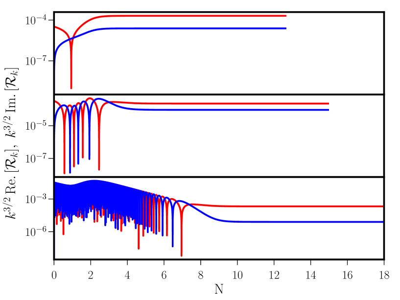
In the case of QP, we choose the initial value of the scalar field to be $\phi_{\mathrm{i}}=18.85\,M_{{}_{\mathrm{Pl}}}$. As we mentioned, the initial velocity of the field is determined by the choice $\epsilon_{1\mathrm{i}}=2.99$. Under these conditions, the best-fit values for the mass $m$ of the scalar field prove to be $6.41\times 10^{-6}\,M_{{}_{\mathrm{Pl}}}$ and $6.17\times 10^{-6}\,M_{{}_{\mathrm{Pl}}}$ in the cases of QPa and QPb, respectively (cf. Tab. 3). Moreover, in these cases, the best-fit values of $N_{\ast}$ turn out to be $55.06$ and $57.32$. For the above parameter values and initial conditions, the scalar field rolls down the potential for about $65$ $e$-folds (counted from $N=0$ when the scalar field is at $\phi_{\mathrm{i}}$), before inflation is terminated close to the minimum of the quadratic potential.

In the case of SMI, we choose the initial value of the scalar field to be $\phi_{\mathrm{i}}=8.37\,M_{{}_{\mathrm{Pl}}}$, with $\epsilon_{1\mathrm{i}}=2.99$. We find that the best-fit values for the parameter $\Lambda$ in the cases of SMIa and SMIb prove to be $9.66\times 10^{-10}\,M_{{}_{\mathrm{Pl}}}^{4}$ and $8.99\times 10^{-10}\,M_{{}_{\mathrm{Pl}}}^{4}$, respectively (cf. Tab. 3). Also, the corresponding best-fit values for $N_{\ast}$ turn out to be $53.22$ and $55.19$. For the above initial conditions and parameter values, we find that inflation ends after approximately $64$ $e$-folds.

Having evolved the background and the perturbations, we evaluate the power spectra at a suitably late time when all the modes of cosmological interest (say, $10^{-5}<k<1\,\mathrm{Mpc}^{-1}$) are sufficiently outside the Hubble radius. One finds that all the scalar and tensor power spectra, generically, exhibit a drop in power on large scales, as illustrated in Fig. 3.

Figure 3: The scalar (on the left) and tensor (on the right) power spectra evaluated either analytically or numerically have been plotted in the various inflationary scenarios of our interest. We have plotted the best-fit power spectra in all the different models we have considered: viz. the cases of the quadratic potential (QPa, QPb and QPc, in blue, green and lime) and the first Starobinsky model (SMIa, SMIb and SMIc, in cyan, orange and purple) with kinetically dominated initial conditions and their duals, the second Starobinsky model (SMII, in brown), punctuated inflation (PI, in black) and the hard cut-off model (HCO, in magenta). For comparison we have also included the best-fit, featureless, nearly scale invariant power law spectra (in red). While most models exhibit a cut-off on large scales, the drop in scalar power is the sharpest in PI than in the other cases. As we shall see, the scalar power spectrum in PI leads to the largest level of improvement in the fit to the CMB data. Moreover, all the models lead to oscillations before the spectra turn nearly scale invariant and, understandably, the amplitude of the oscillations is the smallest in the case of HCO, since it involves only slow roll. Note that, as far as the tensor power spectra are concerned, the scenarios involving SMI predict lower amplitudes than that of QP. Also, the drop in tensor power on large scales in models with initial kinetic domination, their duals and HCO, is similar to what occurs in the case of the the scalar power spectrum. Evidently, this behavior is due to the imposition of the standard initial conditions on the modes when they are in the super-Hubble regime. Besides, we should point out that PI has the lowest tensor power amongst all the models of interest.

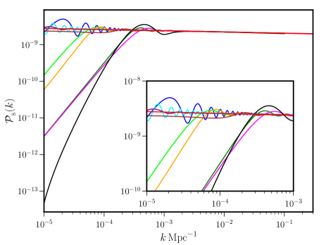
In fact, the suppression in power occurs when the Bunch-Davies initial conditions are imposed over modes that never satisfy the sub-Hubble condition $k>\sqrt{z^{\prime\prime}/z}$ or $k>\sqrt{a^{\prime\prime}/a}$. Moreover, as is expected in any transition, the power spectra exhibit a burst of oscillations before they turn nearly scale invariant on smaller scales. Further, as far as the tensor power spectra are concerned, the scenarios involving the Starobinsky potential lead to a lower tensor power overall, when compared to the quadratic potential. However, there is a small difference in the scale at which the onset of the suppression occurs in the tensor power when compared to the scalar power in a given model. This can be attributed to the difference in the behavior of the quantities $z^{\prime\prime}/z$ and $a^{\prime\prime}/a$ that govern the evolution of the scalar and tensor modes respectively [cf. Eqs. (1) and (4)]. We should point out that similar scalar and tensor power spectra, with lower power on large scales, can also be arrived at in other potentials that permit slow roll inflation (in this context, see App. A).

II.2.2 Another model due to Starobinsky

The second scenario we shall consider is another model due to Starobinsky which is described by the following linear potential with an abrupt change in its slope [26, 42, 43]:

$$V(\phi)=\left\{\begin{array}[]{cc}V_{0}+A_{+}\,\left(\phi-\phi_{0}\right)&\mathrm{for}\leavevmode\nobreak\ \phi>\phi_{0},\\ V_{0}+A_{-}\,\left(\phi-\phi_{0}\right)&\mathrm{for}\leavevmode\nobreak\ \phi<\phi_{0},\\ \end{array}\right.$$ (10)

where $A_{-}\neq A_{+}$. In order to distinguish from the first Starobinsky model, we shall refer to the scenario described by this potential as Starobinsky model II (SMII, hereafter). We should mention here that, to permit numerical analysis, one often works with a smoothened form of the above potential given by [44]

$$V(\phi)=V_{0}+\frac{1}{2}\,\left(A_{+}+A_{-}\right)\,\left(\phi-\phi_{0}\right)+\frac{1}{2}\,\left(A_{+}-A_{-}\right)\,\left(\phi-\phi_{0}\right)\,\tanh{\left(\frac{\phi-\phi_{0}}{\Delta\phi}\right)}.$$ (11)

It is useful here to briefly describe the dynamics that arises in the model. If we work with parameters such that the constant term $V_{0}$ in the potential dominates, then the first slow roll parameter $\epsilon_{1}$ always remains fairly small through most of the evolution. One also finds that, in such a case, there arise two stages of slow roll inflation with a brief period of departure from slow roll. The deviation from slow roll is reflected in the large values of the second and the third slow roll parameters, viz. $\epsilon_{2}$ and $\epsilon_{3}$ (with $\epsilon_{n+1}={\mathrm{d}}\ln\epsilon_{n}/{\mathrm{d}}N$, for $n>1$), which occur briefly when the scalar field crosses $\phi_{0}$. In fact, the small value for $\epsilon_{1}$ permits one to express the scalar modes in terms of the de Sitter modes and thereby evaluate the power spectrum even analytically. It can be shown that the power spectrum in the model can be expressed as [26, 42, 43]

$${\mathcal{P}}_{{}_{\mathrm{S}}}(k) \simeq A_{{}_{\mathrm{S}}}\,\bigg{\{}1-\frac{3\,\Delta A}{A_{+}}\,\frac{k_{0}}{k}\,\left[\left(1-\frac{k_{0}^{2}}{k^{2}}\right)\,\mathrm{sin}\left(\frac{2\,k}{k_{0}}\right)+\frac{2\,k_{0}}{k}\,\mathrm{cos}\left(\frac{2\,k}{k_{0}}\right)\right]$$ (12)

$$+\,\frac{9\,\Delta A^{2}}{2\,A^{2}_{+}}\,\frac{k^{2}_{0}}{k^{2}}\,\left(1+\frac{k_{0}^{2}}{k^{2}}\right)\,\left[1+\frac{k^{2}_{0}}{k^{2}}-\frac{2\,k_{0}}{k}\,\mathrm{sin}\left(\frac{2\,k}{k_{0}}\right)+\left(1-\frac{k_{0}^{2}}{k^{2}}\right)\,\mathrm{cos}\left(\frac{2\,k}{k_{0}}\right)\right]\bigg{\}},\qquad\;\;$$

where we have set $A_{{}_{\mathrm{S}}}=\left[3\,H_{{}_{\mathrm{I}}}^{3}/(2\,\pi\,A_{-})\right]^{2}$, while $\Delta A=A_{-}-A_{+}$ and $H_{{}_{\mathrm{I}}}^{2}\simeq V_{0}/(3\,M_{{}_{\mathrm{Pl}}}^{2})$. Note that, since the above analytical result for the scalar power spectrum has been arrived at using the de Sitter modes, the spectrum is strictly scale invariant on small scales. In order to account for a tilt, while comparing with the CMB data, we multiply the above power spectrum by $(k/k_{\ast})^{n_{{}_{\mathrm{S}}}-1}$. The tensor power spectrum is assumed to be of constant amplitude throughout the range of wave numbers, as the features in the model occur only in the scalar power spectrum. The tensor amplitude is arrived at through a constant tensor-to-scalar ratio $r$, which is defined through the relation ${\mathcal{P}}_{{}_{\mathrm{T}}}=r\,{\mathcal{P}}_{{}_{\mathrm{S}}}(k_{\ast})$, with $k_{\ast}$ being the pivot scale. As we shall discuss later, upon comparing such a spectrum with the CMB data, we obtain the following best-fit values for the parameters involved: $A_{{}_{\mathrm{S}}}=2.11\times 10^{-9}$, $n_{{}_{\mathrm{S}}}=0.97$, $k_{0}=6.32\times 10^{-5}\,{\mathrm{Mpc}^{-1}}$, $\Delta\,A/A_{+}=-0.074$ and $r=0.017$. We have illustrated the best-fit scalar and tensor power spectra in Fig. 3. As should be clear from the figure, the scalar power spectrum exhibits a step-like feature on large scales and is nearly invariant at small scales. It should be pointed out that the height of the step in the power spectrum is essentially determined by the difference in the slopes $A_{+}$ and $A_{-}$.

II.2.3 The punctuated inflationary scenario

The third scenario we shall consider is the so-called punctuated inflationary scenario (referred to hereafter as PI) achieved with the aid of the potential [14, 15]

$$V(\phi)=\frac{1}{2}\,m^{2}\,\phi^{2}-\frac{2}{3}\,m^{2}\,\phi_{0}^{2}\,\left(\frac{\phi}{\phi_{0}}\right)^{3}+\frac{1}{4}\,m^{2}\,\phi_{0}^{2}\,\left(\frac{\phi}{\phi_{0}}\right)^{4}.$$ (13)

The potential contains a point of inflection at $\phi=\phi_{0}$. If one starts with a suitably large initial value of the scalar field such that $\phi\gg\phi_{0}$, the potential admits two stages of slow roll inflation separated by a brief departure (for less than an $e$-fold) from inflation. We shall choose to work with $\phi_{\mathrm{i}}=12.00\,M_{{}_{\mathrm{Pl}}}$ and $\epsilon_{1{\mathrm{i}}}=2\times 10^{-3}$. On setting $\phi_{0}=1.9654\,M_{{}_{\mathrm{Pl}}}$, we obtain the best-fit value for the parameter $m$ to be $7.16\times 10^{-8}\,M_{{}_{\mathrm{Pl}}}$. We have plotted the resulting scalar and tensor power spectra in Fig. 3. Note that the scalar power spectrum exhibits a sharp drop in power on large scales. The model also predicts a very low amplitude for the tensor power throughout the range of wave numbers of interest. However, the model has a major drawback. One finds that, in order for the drop in power to occur at wave numbers roughly corresponding to the Hubble scale today, the largest scale has to leave the Hubble radius during inflation considerably (about $30$–$35$ $e$-folds) earlier than the nominally accepted upper bound of about $65$ $e$-folds, when counted from the end of inflation (for a discussion on this upper bound, see Refs. [45, 46]). For the above values of the parameters, we find that inflation lasts for about $110$ $e$-folds and the pivot scale itself exits the Hubble radius at about $90.61$ $e$-folds before the end of inflation. Despite the drawback, we believe the model is interesting for the reason that, amongst the different models we consider, it leads to the largest improvement in the fit to the CMB data. We shall briefly comment about the model further in concluding section.

II.2.4 The hard cut-off model

It would be interesting to analytically describe the model with kinetically dominated initial conditions and evaluate the corresponding observable quantities of interest. However, it proves to be a bit cumbersome to do so. A simpler model, which permits complete analytical evaluation of the scalar power and bispectra corresponds to a situation wherein the scalar field starts on the inflationary attractor at some given conformal time, say, $\eta_{\mathrm{i}}$. We shall refer to such a scenario as the hard cut-off model (or, simply, HCO). The attractive aspect of the initially kinetically dominated model is that inflation begins naturally at a specific time when the velocity of the scalar field decreases below a threshold value as it rolls down the potential. In contrast, in the hard cut-off model, we have to a priori assume that inflation begins at a specific time with the scalar field being on the attractor.

Since the model involves only slow roll, it is straightforward to arrive at the Fourier modes $f_{k}$ describing the curvature perturbation. As is well known, during slow roll, the scalar mode $f_{k}$, in general, can be expressed in terms of the de Sitter solutions as

$$f_{k}(\eta)=\frac{i\,H_{{}_{\rm I}}}{M_{{}_{\mathrm{Pl}}}\,\sqrt{4\,k^{3}\,\epsilon_{1}}}\,\bigl{[}\alpha_{k}\,(1+i\,k\,\eta)\,{\rm e}^{-i\,k\,\eta}-\beta_{k}\,(1-i\,k\,\eta)\,{\rm e}^{i\,k\,\eta}\bigr{]},$$ (14)

where $H_{{}_{\rm I}}$ represents the Hubble scale during inflation and $\epsilon_{1}$ denotes the first slow roll parameter. The quantities $\alpha_{k}$ and $\beta_{k}$ are the so-called Bogoliubov coefficients. If one imposes the standard Bunch-Davies initial conditions in the sub-Hubble limit, then one will have $\alpha_{k}=1$ and $\beta_{k}=0$. In our case, we shall impose the initial conditions at the time $\eta_{\mathrm{i}}$ irrespective of whether the modes are inside or outside the Hubble radius. In such a case, we obtain the Bogoliubov coefficients $\alpha_{k}$ and $\beta_{k}$ to be

$$\alpha_{k} = 1+\frac{i}{k\,\eta_{\mathrm{i}}}-\frac{1}{2\,k^{2}\,\eta_{\mathrm{i}}^{2}}=1-\frac{i\,k_{\mathrm{i}}}{k}-\frac{k_{\mathrm{i}}^{2}}{2\,k^{2}},$$ (15a)

$$\beta_{k} = -\frac{1}{2\,k^{2}\,\eta_{\mathrm{i}}^{2}}\,{\rm e}^{-2\,i\,k\,\eta_{\mathrm{i}}}=-\frac{k_{\mathrm{i}}^{2}}{2\,k^{2}}\,{\rm e}^{2\,i\,k/k_{\mathrm{i}}},$$ (15b)

where we have set $k_{\mathrm{i}}=-1/\eta_{\mathrm{i}}$. Note that, as $\eta_{\mathrm{i}}\to-\infty$ (i.e. as $k_{\mathrm{i}}\to 0$), $\alpha_{k}\to 1$ and $\beta_{k}\to 0$, which corresponds to the conventional sub-Hubble, Bunch-Davies initial conditions often imposed on all the modes.

With the modes $f_{k}$ at hand, it is now straightforward to evaluate the resulting power spectrum by substituting the modes in the expression (2) and taking the late time (i.e. $\eta\to 0$) limit. One can easily show that the power spectrum can be written as

$${\mathcal{P}}_{{}_{\mathrm{S}}}(k)=A_{{}_{\mathrm{S}}}\,|\alpha_{k}-\beta_{k}|^{2}=A_{{}_{\mathrm{S}}}\,\biggl{[}1+\frac{k_{\mathrm{i}}^{4}}{2\,k^{4}}-\frac{k_{\mathrm{i}}^{3}}{k^{3}}\,\sin\left(\frac{2\,k}{k_{\mathrm{i}}}\right)+\left(\frac{k_{\mathrm{i}}^{2}}{k^{2}}-\frac{k_{\mathrm{i}}^{4}}{2\,k^{4}}\right)\,\cos\left(\frac{2\,k}{k_{\mathrm{i}}}\right)\biggr{]},\quad\;\;$$ (16)

where we have set $A_{{}_{\mathrm{S}}}=H_{{}_{\mathrm{I}}}^{2}/(8\,\pi^{2}\,\epsilon_{1})$. We find that this analytical expression matches the corresponding numerical result very well, say, in QP or SMI, modulo at small scales where the de Sitter modes are not adequate to capture the spectral tilt that arises in a realistic model. Therefore, when comparing the HCO model with the CMB data, to allow for the spectral tilt at small scales, we have multiplied the above scalar power spectrum by $(k/k_{\ast})^{n_{{}_{\mathrm{S}}}-1}$ as in the case of SMII. Moreover, we have defined the tensor power spectrum to be ${\mathcal{P}}_{{}_{\mathrm{T}}}(k)=r\,{\mathcal{P}}_{{}_{\mathrm{S}}}(k)$, with the tensor-to-scalar ration $r$ assumed to be a constant. Such a scale-dependent definition (in contrast to the SMII case, where the tensor power spectrum was scale invariant) is important because the model predicts features in the tensor power spectrum similar to that in the scalar power spectrum, and we have consistently accounted for it in the analysis. We obtain the following best-fit values for the parameters involved: $A_{{}_{\mathrm{S}}}=2.09\times 10^{-9}$, $n_{{}_{\mathrm{S}}}=0.96$, $k_{\mathrm{i}}=2.03\times 10^{-4}\,{\mathrm{Mpc}^{-1}}$, and $r=0.043$. In Fig. 3, we have plotted the analytical scalar and tensor power spectra, with the $(k/k_{\ast})^{n_{{}_{\mathrm{S}}}-1}$ term included, corresponding to the above mentioned best-fit values. Clearly, the power spectra exhibit a suppression of power on large scales as in the case of the other models. As we shall discuss later, the HCO model allows us to evaluate the scalar bispectrum too analytically. The analytical calculations prove to be handy as they permit us to test the numerical results against the analytical results in a situation wherein the Bunch-Davies initial conditions are imposed on super-Hubble scales.

II.2.5 A dual to initial kinetic domination

We shall now discuss a situation which we shall refer to as the dual to the scenario with kinetically dominated initial conditions. Recall that, in the model with initial kinetic domination, the scalar field starts with a large velocity. Evidently, this corresponds to a situation wherein the field begins from a point away from the inflationary attractor. It is interesting to examine the effects on the power spectrum in a scenario with a finite duration of inflation where the field starts with a small velocity (than its value on the attractor) rather than a large velocity. As in the hard cut-off model, there is no natural way of terminating inflation (when one goes back in time) in such a case. Therefore, we shall assume that inflation begins at a specific time and that the Bunch-Davies initial conditions are imposed on super-Hubble scales for a range of modes. A version of such a scenario has been considered previously in the literature and we find that they are referred to as non-attractor models of inflation (in this context, see, for instance, Ref. [47, 48]). Under these conditions, we find that, as the field evolves towards the attractor, there occurs a sharp drop in power on large scales and a regime of oscillations arises over intermediate scales before the spectrum turns nearly scale invariant on small scales. We shall refer to this case as QPc and SMIc when implemented in the quadratic potential (6) and Starobinsky model (7), respectively. In the case of QPc, we choose $\phi_{\mathrm{i}}=16.00\,M_{{}_{\mathrm{Pl}}}$ and $\epsilon_{1\mathrm{i}}=10^{-4}$, which leads to inflation of about $65$ $e$-folds. In the case of SMIc, we work with $\phi_{\mathrm{i}}=5.52\,M_{{}_{\mathrm{Pl}}}$ and $\epsilon_{1\mathrm{i}}=10^{-4}$, which too results in inflation lasting for about $65$ $e$-folds. We find that the best-fit values for the parameter in these models prove to be $m=6.15\times 10^{-6}\,M_{{}_{\mathrm{Pl}}}$ and $V_{0}=8.75\times 10^{-10}\,M_{{}_{\mathrm{Pl}}}^{4}$. The pivot scale exits the Hubble radius at $57.32$ and $55.87$ $e$-folds before the end of inflation in the cases of QPc and SMIc, respectively. In Fig. 3, we have illustrated the power spectra (that lead to the best-fit to the CMB data) in the dual scenario, viz. QPc and SMIc, along with the spectra arising in the cases with initial kinetic domination, i.e. QPa, SMIa, QPb and SMIb (as well as the other models of interest). Clearly, the kinetically dominated model and its dual generate spectra with roughly similar features. We find that the drop in power at large scales have the same shape in both the scenarios and is mostly independent of the initial velocity of the field.

II.3 Performance against the CMB data

We have compared all the models we have described in the previous subsection against the recent Planck data [49]. In this subsection, we shall discuss the assumptions we have made while comparing the models with the CMB data, the priors on the parameters we have worked with and present the final results for the CMB angular power spectrum.

We have taken into account both the scalar and tensor power spectra arising in the models of interest when comparing against the CMB data. We have modified the CAMB package suitably to include the scalar power spectra arising in the models of our interest [50]. We make use of CosmoMC to carry out the comparison of the models with the CMB data and arrive at the respective likelihoods [51]. We have worked with the 2018 release of Planck data, which comprises of the likelihoods of the TT, TE as well as the EE correlations, along with the lensing likelihood [49]. We have included nonlinear lensing in the calculation of the CMB angular power spectra which has a significant effect over small scales. For models with inflationary spectra calculated numerically, we have evaluated the power spectra at $2000$ points over the following range of wave numbers: $10^{-6}\leq k\leq 10\,{\mathrm{Mpc}^{-1}}$. We should mention that, in CAMB, the maximum value of the multipole $\ell$ is set to be $2700$ to compute the CMB angular power spectrum $C_{\ell}$. We perform an MCMC sampling of the posterior distribution of the parameter space using CosmoMC for each model and arrive at the best-fit $\chi^{2}$ and the corresponding set of parameter values using the in-built package called GetDist.

In Tab. 1, we have listed the priors on the four background cosmological parameters that we have worked with.

Parameter	Lower limit	Upper limit
$\Omega_{\mathrm{b}}\,h^{2}$	$0.005$	$0.1$
$\Omega_{\mathrm{c}}\,h^{2}$	$0.001$	$0.99$
$\theta$	$0.5$	$10$
$\tau$	$0.01$	$0.8$

Table 1: The background cosmological parameters which we have varied and the priors that we have worked with. These are the standard set of background parameters that are often considered while comparing with the CMB data [52].

In Tab. 2, we have listed the priors on the parameters describing the various inflationary models of our interest. Previous experience suggests that the drop in power leading to an improved fit to the CMB data is expected to occur around the wave number $k\simeq 10^{-4}\,{\mathrm{Mpc}^{-1}}$. Hence, while choosing the range of priors for the model parameters which determine the location of the drop in the scalar power (such as $N_{\ast}$), we have made sure that the feature occurs over the wave numbers $10^{-5}\lesssim k\lesssim 10^{-3}\,{\mathrm{Mpc}^{-1}}$.

Model	$\mathrm{ln}\,(A_{{}_{\mathrm{S}}}\times 10^{10})$	$n_{{}_{\mathrm{S}}}$	$r$	$\mathrm{log}_{10}(k_{\mathrm{i}}/\mathrm{Mpc}^{-1})$	$\Delta A/A_{+}$
				or $\,\mathrm{log}_{10}(k_{0}/\mathrm{Mpc}^{-1})$
PL	$[1.61,3.91]$	$[0.8,1.2]$	$[0,2]$	-	-
HCO	$[1.61,3.91]$	$[0.8,1.2]$	$[0,2]$	$[-4,-2]$	-
SMII	$[1.61,3.91]$	$[0.8,1.2]$	$[0,2]$	$[-5,-3]$	$[-0.999,0.700]$

Model	$N_{\ast}$	$\mathrm{log}_{10}(10^{10}\,m^{2}/{M_{{}_{\mathrm{Pl}}}^{2}})$	$\mathrm{log}_{10}(10^{10}\,\Lambda/{M_{{}_{\mathrm{Pl}}}^{4}})$
QPa, QPb, QPc	$[50,60]$	$[-0.55,-0.25]$	-
SMIa, SMIb, SMIc	$[50,60]$	-	$[0.8,1.2]$
PI	$[87,93]$	$[-5.20,-3.47]$	-

Table 2: The parameters associated with the different inflationary models of our interest and the priors that we have worked with. The first set (on top) corresponds to models wherein we have made use of the analytical results for the power spectra and the second set (at the bottom) corresponds to models wherein we have evaluated the spectra numerically.

Model	$\mathrm{ln}\,(A_{{}_{\mathrm{S}}}\times 10^{10})$	$n_{{}_{\mathrm{S}}}$	$r$	$\mathrm{log}_{10}(k_{\mathrm{i}}{\,(\mathrm{or})\,}k_{0}/{\rm Mpc}^{-1})$	$(A_{-}-A_{+})/A_{+}$	$\Delta\chi^{2}$
PL	$3.042$	$0.967$	$0.011$	-	-	-
HCO	$3.039$	$0.962$	$0.043$	$-3.692$	-	$-0.096$
SMII	$3.048$	$0.969$	$0.017$	$-4.199$	$-0.074$	$-0.672$

Model	$N_{\ast}$	log${}_{10}(10^{10}m^{2}/{M_{{}_{\mathrm{Pl}}}^{2}})$	log${}_{10}(10^{10}\Lambda/{M_{{}_{\mathrm{Pl}}}^{4}})$	$\Delta\chi^{2}$
QPa	$55.06$	$-0.386$	-	$2.494$
QPb	$57.32$	$-0.419$	-	$-0.384$
QPc	$57.32$	$-0.422$	-	$-0.014$
SMIa	$53.22$	-	$0.985$	$-0.896$
SMIb	$55.19$	-	$0.954$	$-0.880$
SMIc	$55.87$	-	$0.942$	$-1.170$
PI	$90.61$	$-4.290$	-	$-1.746$

Table 3: The best-fit values of the inflationary parameters and the extent of improvement in $\chi^{2}$ with respect to the standard power law case, arrived at by comparing the models with the recent CMB data. As in the previous table, the first set (on top) corresponds to models with analytical forms for the scalar power spectra and the second set (at the bottom) corresponds to those cases wherein the spectra have been evaluated numerically. We have defined $\Delta\chi^{2}=(\chi^{2}_{\mathrm{model}}-\chi^{2}_{{}_{\mathrm{PL}}})$ so that a negative value for $\Delta\chi^{2}$ implies an improvement in the fit with respect to the PL case. Note that PI leads to the largest improvement in the fit to the data. The dataset we have used is the following combination of likelihoods: TT + TE + EE + low $\ell$ + low E + lensing, from the Planck 2018 data release. The models were compared while accounting for tensors as well as non-linear lensing. We should mention that the best-fit value for $\chi^{2}$ in the PL case we have obtained is $\chi^{2}=2\,(1390.928)=2781.856$. The corresponding value quoted by the Planck team is $\chi^{2}=2\,(1391.104)=2782.208$, which is close to the value we obtain [52].

In Tab. 3, we have listed the improvement in the $\chi^{2}$ and the best-fit values for the inflationary parameters for the different models we have considered. Recall that the power law (PL) case corresponds to the simplest situation wherein the scalar power spectrum is expressed as ${\mathcal{P}}_{{}_{\mathrm{S}}}(k)=A_{{}_{\mathrm{S}}}\,(k/k_{\ast})^{n_{{}_{\mathrm{S}}}-1}$. For the PL case, the $\chi^{2}$ we obtain from the GetDist package is $2781.856$, while the value quoted by the Planck team is $2782.208$. Note that the quantity $\Delta\chi^{2}$ is the difference in $\chi^{2}$ between a given inflationary model and the PL case, with a negative value indicating an improvement in the fit to the data. Evidently, PI leads to the largest improvement in the fit to the data. Earlier, in Fig. 3, we had plotted the inflationary scalar power spectra for parameter values of the various models that lead to the best fit to the CMB data. In Fig. 4, we have plotted the corresponding CMB angular power spectra for three of the models which lead to reasonable levels of improvement (with $\Delta\chi^{2}\simeq 0.6\mbox{--}1.7$) in their fit to the data.

Figure 4: The best-fit CMB angular power spectra have been plotted for the three models SMIc (in blue), SMII (in green) and PI (in cyan) which lead to an improvement in $\Delta\chi^{2}$ of $0.6\mbox{--}1.7$ in the fit to the recent Planck data. In order to highlight the differences, we have also plotted the best-fit angular power spectrum for the PL case (in red). We have also included the Planck 2018 data points along with their error bars (in black). Note that the multipoles $\ell$ appear on a log scale until $\ell=32$ (indicated by the vertical line) and on a linear scale for $\ell>32$. We should point out the fact that the CMB angular spectrum in the case of PI exhibits an oscillation over the lower multipoles before it merges with, say, the result for the power law case, at the higher multipoles. The angular spectra for the models of SMIc and SMII are suppressed to a far less extent when compared to the spectrum of PI over the low multipoles (as highlighted in the inset).

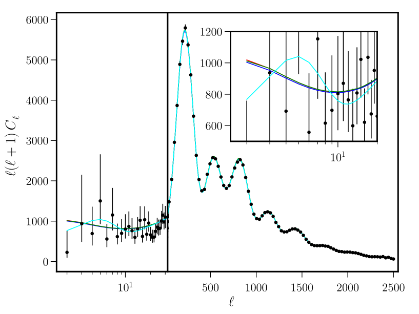
Lastly, we should mention that, in App. B, we have illustrated the marginalized posterior distribution on the inflationary parameters in the models SMIc, PI and SMII. We have also illustrated the constraints on the Hubble parameter $H_{0}$ that one obtains in these cases. Interestingly, we find that, though PI modestly improves the fit to the CMB data, it seems to exacerbate the so-called Hubble tension, a topic that is considerable interest today [53, 54].

Having described the alternative scenarios resulting in scalar spectra with a sharp drop in power on large scales, let us now turn to the evaluation of the scalar non-Gaussianities in these models.

III The third order action and the surface terms

In order to evaluate the scalar bispectrum, one requires the action describing the curvature perturbation at the third order. It can be shown that, at the third order, the action governing the curvature perturbation ${\mathcal{R}}$ can be expressed as (see, for instance, Refs. [55, 56, 43, 57])

$$\delta S_{3}[{\mathcal{R}}] = M_{{}_{\mathrm{Pl}}}^{2}\,\int_{\eta_{\mathrm{i}}}^{\eta_{\mathrm{e}}}\,{\mathrm{d}}\eta\,\int{\mathrm{d}}^{3}{\bm{x}}\,\biggl{[}a^{2}\,\epsilon_{1}^{2}\,{\mathcal{R}}\,{\mathcal{R}}^{\prime 2}+a^{2}\,\epsilon_{1}^{2}\,{\mathcal{R}}\,({\partial}{\mathcal{R}})^{2}-2\,a\,\epsilon_{1}\,{\mathcal{R}}^{\prime}\,({\partial}{\mathcal{R}})\,(\partial\chi)$$ (17)

$$+\,\frac{a^{2}}{2}\,\epsilon_{1}\,\epsilon_{2}^{\prime}\,{\mathcal{R}}^{2}\,{\mathcal{R}}^{\prime}+\frac{\epsilon_{1}}{2}\,({\partial}{\mathcal{R}})\,({\partial}\chi)\,\partial^{2}\chi+\frac{\epsilon_{1}}{4}\,{\partial}^{2}{\mathcal{R}}\,(\partial\chi)^{2}+2\,{\cal F}({\mathcal{R}})\,\frac{\delta{\cal L}_{2}}{\delta{\mathcal{R}}}\biggr{]},$$

where, as we have mentioned earlier, $\epsilon_{2}={\mathrm{d}}\,{\rm ln}\,\epsilon_{1}/{\mathrm{d}}N$ is the second slow roll parameter, while ${\partial}^{2}\chi=a\,\epsilon_{1}\,{\mathcal{R}}^{\prime}$. The quantity ${\cal F}$(${\mathcal{R}}$) is given by

$${\cal F}({\mathcal{R}}) = \frac{\epsilon_{2}}{4}\,{\mathcal{R}}^{2}+\frac{1}{a\,H}\,{\mathcal{R}}\,{\mathcal{R}}^{\prime}+\frac{1}{4\,a^{2}\,H^{2}}\biggl{\{}-({\partial}{\mathcal{R}})\,({\partial}{\mathcal{R}})+{\partial}^{-2}[{\partial}_{i}\,{\partial}_{j}\,({\partial}_{i}{\mathcal{R}}\,{\partial}_{j}{\mathcal{R}})]\biggr{\}}$$ (18)

$$+\,\frac{1}{2\,a^{2}\,H}\biggl{\{}({\partial}{\mathcal{R}})\,({\partial}\chi)-\partial^{-2}[{\partial}_{i}\,\partial_{j}\,({\partial}_{i}{\mathcal{R}}\,{\partial}_{j}\chi)]\biggr{\}}$$

and ${\cal L}_{2}$ denotes the Lagrangian density associated with the action governing the curvature perturbation at the second order. Note that $\eta_{\mathrm{i}}$ is the conformal time when the initial conditions are imposed on the perturbations and $\eta_{\mathrm{e}}$ is the conformal time close to the end of inflation, when the power and bispectra are evaluated. Typically, in analytical calculations, one assumes that $\eta_{\mathrm{i}}\to-\infty$ and $\eta_{\mathrm{e}}\to 0^{-}$.

The third order action (17) is arrived at from the original action governing the system of the gravitational and scalar fields. A set of temporal and spatial boundary terms are often ignored in arriving at the above action [55, 56, 57]. The spatial boundary terms do not contribute to the scalar bispectrum under any condition. However, in cases such as the scenario involving inflation of a finite duration, one finds that the temporal boundary terms can contribute non-trivially. These temporal boundary terms are given by [57]

$$\delta S^{\rm B}_{3}[{\mathcal{R}}] = M_{{}_{\mathrm{Pl}}}^{2}\,\int_{\eta_{\mathrm{i}}}^{\eta_{\mathrm{e}}}{\mathrm{d}}\eta\,\int{\mathrm{d}}^{3}{\bm{x}}\;\frac{{\mathrm{d}}}{{\mathrm{d}}\eta}\biggl{\{}-9\,a^{3}H\,{\mathcal{R}}^{3}+\frac{a}{H}\,(1-\epsilon_{1})\,{\mathcal{R}}\,({\partial}{\mathcal{R}})^{2}-\frac{1}{4\,a\,H^{3}}\,({\partial}{\mathcal{R}})^{2}\,{\partial}^{2}{\mathcal{R}}$$ (19)

$$-\frac{a\,\epsilon_{1}}{H}\,{\mathcal{R}}\,{\mathcal{R}}^{\prime 2}-\,\frac{a\,\epsilon_{2}}{2}\,{\mathcal{R}}^{2}\,{\partial}^{2}\chi+\frac{1}{2\,a\,H^{2}}\,{\mathcal{R}}\,\left({\partial}_{i}{\partial}_{j}{\mathcal{R}}\,{\partial}_{i}{\partial}_{j}\chi-\partial^{2}{\mathcal{R}}\,\partial^{2}\chi\right)$$

$$-\,\frac{1}{2\,aH}\,{\mathcal{R}}\,\left[{\partial}_{i}{\partial}_{j}\chi\,{\partial}_{i}{\partial}_{j}\chi-({\partial}^{2}\chi)^{2}\right]\biggr{\}}.$$

It should be mentioned here that, in standard slow roll inflation, apart from the term involving $\epsilon_{2}$, none of the above terms contribute either at early or at late times. The term involving $\epsilon_{2}$ contributes non-trivially at late times, and this contribution is often absorbed through a field redefinition (in this context, see, for example, Refs. [55, 57]). However, it is important to clarify that, in this work, we do not carry out any field redefinition. We shall explicitly calculate all the contributions due to the bulk and the boundary terms (17) and (19).

IV Evaluating the scalar bispectrum

In this section, we shall describe the numerical evaluation of the scalar bispectrum and the corresponding non-Gaussianity parameter $f_{{}_{\mathrm{NL}}}$ in the different models of our interest. In fact, these quantities have been calculated earlier in the cases of the second Starobinsky model and punctuated inflation (in this context, see, for example, Refs. [43, 38, 58]). We should mention here that, in an earlier work, we had briefly presented the main results for the scalar bispectrum in models with kinetic dominated initial conditions [27]. These models wherein the initial conditions are imposed on super-Hubble scales pose certain challenges and it is instructive to compare the numerical procedure for the computation of the bispectrum and the non-Gaussianity parameter $f_{{}_{\mathrm{NL}}}$ in the different cases.

IV.1 The scalar bispectrum and the non-Gaussianity parameter

Let us begin by recalling a few essential points regarding the scalar bispectrum $G({\bm{k}}_{1},{\bm{k}}_{2},{\bm{k}}_{3})$ and the corresponding non-Gaussianity parameter $f_{{}_{\mathrm{NL}}}({\bm{k}}_{1},{\bm{k}}_{2},{\bm{k}}_{3})$, where the three wavevectors ${\bm{k}}_{1}$, ${\bm{k}}_{2}$ and ${\bm{k}}_{3}$ form the edges of a triangle. In the single field inflationary scenarios of our interest, the scalar bispectrum is essentially the three-point function of the curvature perturbation in Fourier space. The bispectrum can be arrived at by using the third order action describing the curvature perturbation we discussed in the previous section and the standard rules of perturbative quantum field theory [55, 56, 43, 57].

It can be shown that the scalar bispectrum can be expressed as (see, for instance, Refs. [43, 38])

$$G({\bm{k}}_{1},{\bm{k}}_{2},{\bm{k}}_{3}) = \sum_{C=1}^{9}\;G_{{}_{C}}({\bm{k}}_{1},{\bm{k}}_{2},{\bm{k}}_{3})$$ (20)

$$= M_{{}_{\mathrm{Pl}}}^{2}\;\sum_{C=1}^{6}\;\Biggl{[}f_{k_{1}}(\eta_{\mathrm{e}})\,f_{k_{2}}(\eta_{\mathrm{e}})\,f_{k_{3}}(\eta_{\mathrm{e}})\,{\mathcal{G}}_{{}_{C}}({\bm{k}}_{1},{\bm{k}}_{2},{\bm{k}}_{3})+{\rm complex\;conjugate}\Biggr{]}$$

$$+\,G_{7}({\bm{k}}_{1},{\bm{k}}_{2},{\bm{k}}_{3})+\,G_{8}({\bm{k}}_{1},{\bm{k}}_{2},{\bm{k}}_{3})+G_{9}({\bm{k}}_{1},{\bm{k}}_{2},{\bm{k}}_{3}),$$

where, as we mentioned earlier, $f_{k}$ are the Fourier modes of the curvature perturbation [cf. Eq. (3)], while $\eta_{\mathrm{e}}$ denotes the conformal time close to the end of inflation. The quantities ${\mathcal{G}}_{{}_{C}}({\bm{k}}_{1},{\bm{k}}_{2},{\bm{k}}_{3})$ represent six integrals that involve the scale factor, the slow roll parameters, the modes $f_{k}$ and their time derivatives $f_{k}^{\prime}$. They correspond to the six bulk terms appearing in the cubic order action (17) and are described by the following expressions:

$${\mathcal{G}}_{1}({\bm{k}}_{1},{\bm{k}}_{2},{\bm{k}}_{3}) = 2\,i\,\int_{\eta_{\mathrm{i}}}^{\eta_{\mathrm{e}}}{\mathrm{d}}\eta\;a^{2}\,\epsilon_{1}^{2}\,\biggl{(}f_{k_{1}}^{\ast}\,f_{k_{2}}^{\prime\ast}\,f_{k_{3}}^{\prime\ast}+{\rm two\leavevmode\nobreak\ permutations}\biggr{)},$$ (21a)

$${\mathcal{G}}_{2}({\bm{k}}_{1},{\bm{k}}_{2},{\bm{k}}_{3}) = -2\,i\;\left({\bm{k}}_{1}\cdot{\bm{k}}_{2}+\,{\rm two\leavevmode\nobreak\ permutations}\right)\,\int_{\eta_{\mathrm{i}}}^{\eta_{\mathrm{e}}}{\mathrm{d}}\eta\;a^{2}\,\epsilon_{1}^{2}\,f_{k_{1}}^{\ast}\,f_{k_{2}}^{\ast}\,f_{k_{3}}^{\ast},$$ (21b)

$${\mathcal{G}}_{3}({\bm{k}}_{1},{\bm{k}}_{2},{\bm{k}}_{3}) = -2\,i\,\int_{\eta_{\mathrm{i}}}^{\eta_{\mathrm{e}}}{\mathrm{d}}\eta\;a^{2}\,\epsilon_{1}^{2}\,\biggl{(}\frac{{\bm{k}}_{1}\cdot{\bm{k}}_{2}}{k_{2}^{2}}\,f_{k_{1}}^{\ast}\,f_{k_{2}}^{\prime\ast}\,f_{k_{3}}^{\prime\ast}+{\rm five\leavevmode\nobreak\ permutations}\biggr{)},$$ (21c)

$${\mathcal{G}}_{4}({\bm{k}}_{1},{\bm{k}}_{2},{\bm{k}}_{3}) = i\,\int_{\eta_{\mathrm{i}}}^{\eta_{\mathrm{e}}}{\mathrm{d}}\eta\;a^{2}\,\epsilon_{1}\,\epsilon_{2}^{\prime}\,\biggl{(}f_{k_{1}}^{\ast}\,f_{k_{2}}^{\ast}\,f_{k_{3}}^{\prime\ast}+{\rm two\leavevmode\nobreak\ permutations}\biggr{)},$$ (21d)

$${\mathcal{G}}_{5}({\bm{k}}_{1},{\bm{k}}_{2},{\bm{k}}_{3}) = \frac{i}{2}\,\int_{\eta_{\mathrm{i}}}^{\eta_{\mathrm{e}}}{\mathrm{d}}\eta\;a^{2}\,\epsilon_{1}^{3}\;\biggl{(}\frac{{\bm{k}}_{1}\cdot{\bm{k}}_{2}}{k_{2}^{2}}\,f_{k_{1}}^{\ast}\,f_{k_{2}}^{\prime\ast}\,f_{k_{3}}^{\prime\ast}+{\rm five\leavevmode\nobreak\ permutations}\biggr{)},$$ (21e)

$${\mathcal{G}}_{6}({\bm{k}}_{1},{\bm{k}}_{2},{\bm{k}}_{3}) = \frac{i}{2}\,\int_{\eta_{\mathrm{i}}}^{\eta_{\mathrm{e}}}{\mathrm{d}}\eta\,a^{2}\,\epsilon_{1}^{3}\,\biggl{(}\frac{k_{1}^{2}\,\left({\bm{k}}_{2}\cdot{\bm{k}}_{3}\right)}{k_{2}^{2}\,k_{3}^{2}}\,f_{k_{1}}^{\ast}\,f_{k_{2}}^{\prime\ast}\,f_{k_{3}}^{\prime\ast}+{\rm two\leavevmode\nobreak\ permutations}\biggr{)}.$$ (21f)

These integrals are to be evaluated from a sufficiently early time ($\eta_{\mathrm{i}}$), when the modes are typically well inside the Hubble radius, until very late times, which can be conveniently chosen to be a time close to the end of inflation ($\eta_{\mathrm{e}}$). We should mention here that the last term in action (17) involving ${\cal F}({\mathcal{R}})\,({\delta{\cal L}_{2}}/{\delta{\mathcal{R}}})$ actually vanishes when we assume that the curvature perturbation satisfies the linear equation of motion [cf. Eqs. (3) and (1)].

In the expression (20) for the scalar bispectrum, the terms $G_{7}({\bm{k}}_{1},{\bm{k}}_{2},{\bm{k}}_{3})$, $G_{8}({\bm{k}}_{1},{\bm{k}}_{2},{\bm{k}}_{3})$ and $G_{9}({\bm{k}}_{1},{\bm{k}}_{2},{\bm{k}}_{3})$ are the contributions that arise due to the boundary terms (19) associated with the third order action governing the curvature perturbation. The contribution $G_{7}({\bm{k}}_{1},{\bm{k}}_{2},{\bm{k}}_{3})$ is due to the term containing $\epsilon_{2}$ in the boundary terms (19) and it can be expressed as

$$G_{7}({\bm{k}}_{1},{\bm{k}}_{2},{\bm{k}}_{3}) = -i\,M_{{}_{\mathrm{Pl}}}^{2}\,(f_{k_{1}}(\eta_{\mathrm{e}})\,f_{k_{2}}(\eta_{\mathrm{e}})\,f_{k_{3}}(\eta_{\mathrm{e}}))$$ (22)

$$\times\,\biggl{[}a^{2}\epsilon_{1}\epsilon_{2}\,f_{k_{1}}^{\ast}(\eta)\,f_{k_{2}}^{\ast}(\eta)\,f_{k_{3}}^{\prime\ast}(\eta)+{\rm two\leavevmode\nobreak\ permutations}\biggr{]}_{\eta_{i}}^{\eta_{\mathrm{e}}}$$

$$+\leavevmode\nobreak\ {\rm complex\leavevmode\nobreak\ conjugate}.$$

In standard slow roll inflation, the contribution due to $\eta_{\mathrm{i}}$ vanishes with the introduction of the regulator, and it is only the term evaluated towards end of inflation that contributes. Amongst the boundary terms, we have chosen to write this term separately as it is this contribution that is often taken into account (in slow roll inflation) through a field redefinition [55, 43, 57]. However, as we had mentioned, we do not carry out any field redefinition and explicitly calculate the contributions due to the bulk as well as the boundary terms.

The two terms $G_{8}({\bm{k}}_{1},{\bm{k}}_{2},{\bm{k}}_{3})$ and $G_{9}({\bm{k}}_{1},{\bm{k}}_{2},{\bm{k}}_{3})$ are the contributions due to the remaining temporal boundary terms of the cubic order action listed in Eq. (19). The contributions $G_{9}({\bm{k}}_{1},{\bm{k}}_{2},{\bm{k}}_{3})$ and $G_{8}({\bm{k}}_{1},{\bm{k}}_{2},{\bm{k}}_{3})$ arise due to terms with and without ${\mathcal{R}}^{\prime}$, respectively. They are given by the following expressions:

$$G_{8}({\bm{k}}_{1},{\bm{k}}_{2},{\bm{k}}_{3}) = i\,M_{{}_{\mathrm{Pl}}}^{2}\,f_{k_{1}}(\eta_{\mathrm{e}})\,f_{k_{2}}(\eta_{\mathrm{e}})\,f_{k_{3}}(\eta_{\mathrm{e}})\,\left[\frac{a}{H}\,f_{k_{1}}^{\ast}(\eta)\,f_{k_{2}}^{\ast}(\eta)\,f_{k_{3}}^{\ast}(\eta)\right]_{\eta_{\mathrm{i}}}$$ (23a)

$$\times\,\Biggl{\{}54\,(a\,H)^{2}+\,2\,(1-\epsilon_{1})\,({\bm{k}}_{1}\cdot{\bm{k}}_{2}+{\bm{k}}_{1}\cdot{\bm{k}}_{3}+{\bm{k}}_{2}\cdot{\bm{k}}_{3})$$

$$+\,\frac{1}{2\,(a\,H)^{2}}\,\biggl{[}({\bm{k}}_{1}\cdot{\bm{k}}_{2})\,{k_{3}}^{2}+({\bm{k}}_{1}\cdot{\bm{k}}_{3})\,{k_{2}}^{2}+({\bm{k}}_{2}\cdot{\bm{k}}_{3})\,{k_{1}}^{2}\biggl{]}\Biggr{\}}_{\eta_{\mathrm{i}}}$$

$$+\,{\rm complex\leavevmode\nobreak\ conjugate},$$

$$G_{9}({\bm{k}}_{1},{\bm{k}}_{2},{\bm{k}}_{3}) = i\,M_{{}_{\mathrm{Pl}}}^{2}\,f_{k_{1}}(\eta_{\mathrm{e}})\,f_{k_{2}}(\eta_{\mathrm{e}})\,f_{k_{3}}(\eta_{\mathrm{e}})$$ (23b)

$$\times\Bigg{\{}\frac{\epsilon_{1}}{2\,H^{2}}\,f_{k_{1}}^{\ast}(\eta)\,f_{k_{2}}^{\ast}(\eta)\,f_{k_{3}}^{\prime\ast}(\eta)\,\biggl{[}k_{1}^{2}+k_{2}^{2}-\left(\frac{{\bm{k}}_{1}\cdot{\bm{k}}_{3}}{k_{3}}\right)^{2}-\ \left(\frac{{\bm{k}}_{2}\cdot{\bm{k}}_{3}}{k_{3}}\right)^{2}\biggr{]}$$

$$-\,\frac{a\,\epsilon_{1}}{H}\,f_{k_{1}}^{\ast}(\eta)\,f_{k_{2}}^{\prime\ast}(\eta)\,f_{k_{3}}^{\prime\ast}(\eta)\,\left[2-\epsilon_{1}+\epsilon_{1}\,\left(\frac{{\bm{k}}_{2}\cdot{\bm{k}}_{3}}{k_{2}\,k_{3}}\right)^{2}\right]\Bigg{\}}_{\eta_{\mathrm{i}}}^{\eta_{\mathrm{e}}}$$

$$+\,{\rm two\leavevmode\nobreak\ permutations}+{\rm complex\leavevmode\nobreak\ conjugate}.$$

Note that, because $G_{8}({\bm{k}}_{1},{\bm{k}}_{2},{\bm{k}}_{3})$ involves only ${\mathcal{R}}$ (and not ${\mathcal{R}}^{\prime}$), its contribution at late times (i.e. at $\eta_{\mathrm{e}}$) vanishes identically in any scenario. Moreover, both the boundary terms $G_{8}({\bm{k}}_{1},{\bm{k}}_{2},{\bm{k}}_{3})$ and $G_{9}({\bm{k}}_{1},{\bm{k}}_{2},{\bm{k}}_{3})$ generally do not contribute in inflationary scenarios that do not have a finite duration. But, as we shall see, in the models with kinetically dominated initial regimes, these boundary terms can contribute significantly at the initial time $\eta_{\mathrm{i}}$.

The non-Gaussianity parameter $f_{{}_{\mathrm{NL}}}({\bm{k}}_{1},{\bm{k}}_{2},{\bm{k}}_{3})$ corresponding to the scalar bispectrum $G({\bm{k}}_{1},{\bm{k}}_{2},{\bm{k}}_{3})$ is defined as (see, for instance, Refs. [43, 38])

$$f_{{}_{\mathrm{NL}}}({\bm{k}}_{1},{\bm{k}}_{2},{\bm{k}}_{3}) = -\frac{10}{3}\,\frac{1}{\left(2\,\pi\right)^{4}}\;k_{1}^{3}\,k_{2}^{3}\,k_{3}^{3}\;G({\bm{k}}_{1},{\bm{k}}_{2},{\bm{k}}_{3})$$ (24)

$$\times\,\biggl{[}k_{1}^{3}\,{\mathcal{P}}_{{}_{\mathrm{S}}}(k_{2})\,{\mathcal{P}}_{{}_{\mathrm{S}}}(k_{3})+{\rm two\leavevmode\nobreak\ permutations}\biggr{]}^{-1},$$

where ${\mathcal{P}}_{{}_{\mathrm{S}}}(k)$ denotes the scalar power spectrum [cf. Eq. (2)].

IV.2 Numerical computation of the scalar bispectrum

Let us now discuss the numerical evaluation of the scalar bispectrum. Once the background evolution has been determined, it is a matter of arriving at the solution for the modes $f_{k}$ and then using them to compute the integrals ${\mathcal{G}}_{{}_{C}}({\bm{k}}_{1},{\bm{k}}_{2},{\bm{k}}_{3})$ [cf. Eqs. (21)] and the corresponding contributions to the bispectrum. Evidently, evaluating the contributions due to the boundary terms $G_{7}({\bm{k}}_{1},{\bm{k}}_{2},{\bm{k}}_{3})$, $G_{8}({\bm{k}}_{1},{\bm{k}}_{2},{\bm{k}}_{3})$ and $G_{9}({\bm{k}}_{1},{\bm{k}}_{2},{\bm{k}}_{3})$ [cf. Eqs. (22) and (23)] is relatively straightforward as it involves no integrals and can be arrived at from the background quantities and the modes $f_{k}$.

As we had discussed earlier, in the standard slow roll scenario or in situations involving brief intermediate departures from slow roll [such as in the second Starobinsky model (SMII) and punctuated inflation (PI)], to arrive at the scalar power spectrum, the modes $f_{k}$ are evolved from the time when $k=10^{2}\,\sqrt{z^{\prime\prime}/z}$ to the time when $k=10^{-5}\,\sqrt{z^{\prime\prime}/z}$. It has been established that it is often adequate to consider the evolution of modes over this domain to arrive at the bispectra as well (see Refs. [37, 38, 58]; in this context, also see Refs. [59, 60]). Since the amplitude of curvature perturbation freezes on super-Hubble scales, one finds that the contribution over the domain $k<10^{-5}\,\sqrt{z^{\prime\prime}/z}$ proves to be insignificant. However, as the bispectrum involves three modes, one has to evolve the modes and carry out the integrals from a domain when the smallest of the three wave numbers $(k_{1},k_{2},k_{3})$ satisfies the sub-Hubble condition $k=10^{2}\,\sqrt{z^{\prime\prime}/z}$ until the time when the largest of the three satisfy the super-Hubble condition $k=10^{-5}\,\sqrt{z^{\prime\prime}/z}$.

In fact, there is yet another point one needs to take into account when computing the integrals. Since the modes oscillate in the sub-Hubble domain, one actually needs to introduce a cut-off in order to regulate the integrals involved. Theoretically, such a cut-off is necessary to identify the correct perturbative vacuum (see, for instance, Refs. [55, 56]). Numerically, the cut-off helps us to efficiently compute the integrals. For an arbitrary triangular configuration of the wave vectors, one often works with a democratic cut-off of the form ${\rm exp}\,[-\kappa\,(k_{1}+k_{2}+k_{3})/(3\,\sqrt{z^{\prime\prime}/z})]$, where $\kappa$ is a suitably chosen constant. The value of $\kappa$ is determined by calculating the integrals starting from different times inside the Hubble radius and examining the dependence of the results for the integrals on the initial time and the value of $\kappa$. It is found that, in most of the cases, if one chooses to integrate from $k=10^{2}\,\sqrt{z^{\prime\prime}/z}$, the value of $\kappa\simeq 0.3$ proves to be optimal [38, 58, 59, 60]. In other words, for $\kappa=0.3$, the values of the integrals prove to be independent of how deep inside the Hubble radius the integrals are carried out from. We use this procedure to calculate the integrals ${\mathcal{G}}_{{}_{C}}({\bm{k}}_{1},{\bm{k}}_{2},{\bm{k}}_{3})$ [cf. Eqs. (21)], the resulting bispectrum $G({\bm{k}}_{1},{\bm{k}}_{2},{\bm{k}}_{3})$ and the corresponding non-Gaussianity parameter $f_{{}_{\mathrm{NL}}}({\bm{k}}_{1},{\bm{k}}_{2},{\bm{k}}_{3})$ in the cases of SMII and PI [38].

But, the scenario with kinetically dominated initial conditions and variations of it such as its dual and the hard cut-off model pose a peculiar problem. Recall that, in these cases, modes over a certain range of wave numbers are never inside the Hubble radius (in this context, see Fig. 1). Therefore, the integrals involving modes over this range do not actually require a cut-off. For these modes, we evaluate the integrals from $N=0$ or $N=N_{1}$ when we begin to evolve the perturbations. When we do so, we find that, the contributions to the scalar bispectrum for this range of modes are completely insensitive to the value of the cut-off parameter $\kappa$. This point is illustrated in Fig. 5 wherein we have plotted the contributions to the bispectrum in the equilateral limit (i.e. when $k_{1}=k_{2}=k_{3}=k$) due to the bulk and the boundary terms as a function of $\kappa$ in the case of QPa.

Figure 5: The bulk and the boundary contributions to the scalar bispectrum evaluated numerically in the equilateral limit for the case of the quadratic potential with kinetically dominated initial conditions have been plotted as functions of the cut-off parameter $\kappa$. For highlighting the points we wish to make, we have grouped the six standard bulk terms, along with the seventh term, viz. $G_{{}_{C}}(k)$ with $C=\left\{1,2,\ldots,7\right\}$ (in red) and the boundary terms, viz. $G_{8}(k)$ and $G_{9}(k)$ (in blue). We have plotted these quantities for two modes with the wave numbers $k=5\times 10^{-5}\,{\mathrm{Mpc}^{-1}}$ (in the top panel) and $k=0.1\,{\mathrm{Mpc}^{-1}}$ (in the bottom panel) in the case of the model QPa. The first of these wave numbers is representative of the modes with suppressed power and is always outside the Hubble radius, whereas the second corresponds to a typical mode in the nearly scale invariant regime that emerges from sufficiently deep inside the sub-Hubble domain (cf. Fig. 1). We have plotted the quantities when the integrals involved have been evaluated from $N=0$ (as solid curves) and from the $e$-folds satisfying the conditions $k=100\,\sqrt{z^{\prime\prime}/z}$ and $k=200\,\sqrt{z^{\prime\prime}/z}$ (as dashed and dotted curves, respectively), with the latter two being, evidently, possible only for the mode with the larger wave number. Note that, while the quantities are completely insensitive to $\kappa$ for the first mode, the plots suggest the optimal value of the cut-off parameter to be $\kappa=0.3$ for the second mode. Also, we should point out that the boundary terms dominate the bulk for the mode with the smaller wave number (cf. top panel). Moreover, in the case of the mode with the larger wave number, for $\kappa=0.3$, the boundary terms cease to be important and the contributions to the bispectrum are dominated by the bulk terms, as is expected for a mode that emerges from sufficiently deep inside the Hubble radius.

Also, in QPa and similar scenarios, for the initial conditions and the best-fit values of the parameters we have worked with, we find that we can impose the Bunch-Davies initial condition at $k=10^{2}\,\sqrt{z^{\prime\prime}/z}$ for modes with $k\gtrsim 8\times 10^{-3}\,{\mathrm{Mpc}^{-1}}$ (in this context, see Fig. 1). As one would have expected, for these modes, the choice of $\kappa=0.3$ turns out to be ideal as in the cases of SMII and PI (see Fig. 5). However, since the modes over the range $8\times 10^{-5}\lesssim k\lesssim 8\times 10^{-3}\,{\mathrm{Mpc}^{-1}}$ do not spend an adequate amount of time in the sub-Hubble domain, we are unable to carry out the exercise described above for identifying an apt value of $\kappa$ over this set of wave numbers. We choose to be democratic, and we work with $\kappa=0.3$ over this range of modes as well. Also, we carry out the integrals from $N=0$ or $N=N_{1}$ for all the modes (viz. for $10^{-5}<k<1\,{\rm Mpc}^{-1}$) until the time when the largest of the three wave numbers involved satisfies the condition $k=10^{-5}\,\sqrt{z^{\prime\prime}/z}$.

In Fig. 6, we have plotted the various bulk and boundary contributions to the bispectrum for QPa, SMII and PI.

Figure 6: The different contributions to the scalar bispectrum in the equilateral limit, viz. the bulk terms $G_{1}(k)+G_{3}(k)$ (in red), $G_{2}(k)$ (in blue), $G_{4}(k)+G_{7}(k)$ (in green), $G_{5}(k)+G_{6}(k)$ (in purple) and the boundary terms $G_{8}(k)$ (in cyan) and $G_{9}(k)$ (in orange), evaluated numerically, have been plotted for three models of our interest, viz, QPa (on top), PI (in the middle) and SMII (at the bottom). We should mention that we have made use of the smoothened potential (11) to evaluate the results numerically in the case of SMII. Note that, since all the modes of cosmological interest emerge from sufficiently inside the Hubble radius in SMII and PI, there arise no contributions from the boundary terms in these cases. However, in the case of QPa, it should be clear that the boundary terms dominate at small wave numbers. An interesting point to note regarding PI is that the contribution to the scalar bispectrum due to $G_{4}(k)+G_{7}(k)$ is much higher in magnitude when compared to the contribution $G_{1}(k)+G_{2}(k)+G_{3}(k)$ over small scales. This is due to the fact that the value of $\epsilon_{2}$ is relatively larger than $\epsilon_{1}$ during late times in the model. Hence, the contributions proportional to $\epsilon_{2}$ dominate over others that are proportional to $\epsilon_{1}$. We should also point out the linear growth in $G_{4}(k)+G_{7}(k)$ at large $k$ in SMII. The growth is known to become indefinite in the limit when the quantity $\Delta\phi$ in the potential (11) vanishes, i.e. when the change in the slope of the potential ceases to be smooth and is infinitely abrupt as in the original potential (10) [42, 44].

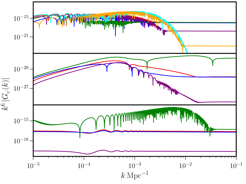
One finds that, in the equilateral limit, the contributions due to the first and the third terms and the contributions due to the fifth and the sixth terms have the same form. Therefore, in the figure, we have plotted the combinations $G_{1}(k)+G_{3}(k)$, $G_{2}(k)$, $G_{4}(k)+G_{7}(k)$, $G_{5}(k)+G_{6}(k)$, $G_{8}(k)$ and $G_{9}(k)$. In the cases of SMII and PI, the boundary terms do not contribute due to the fact that all the modes of interest emerge from well within the Hubble radius. Also, in these two models, as is well known, it is the contribution due to the term $G_{4}(k)+G_{7}(k)$ that dominates [38, 58]. This is easy to understand as the term $G_{4}(k)$ depends on $\epsilon_{2}^{\prime}$ which grows large for a brief period of time in these scenarios. In complete contrast, in QPa, one finds that all the contributions to the bispectrum are roughly of the same order over a wide range of wave numbers. Moreover, in SMII and PI, all the contributions to the bispectrum are enhanced over wave numbers that leave the Hubble radius during the period of departure from slow roll inflation. However, in the case of QPa, the contributions to the scalar bispectrum due to the boundary terms dominate the contributions due to the bulk terms over a range of large scale modes. This is a novel result that does not seem to have been noticed earlier in the literature [27].

IV.3 Analytical calculation in the hard cut-off model

Since it involves only slow roll, the hard cut-off model (HCO) provides a simple situation to evaluate the scalar bispectrum analytically. In this section, we shall compare the analytical results in this case with the corresponding numerical results to highlight the accuracy of our numerical computations in situations wherein the initial conditions for a range of modes are imposed on super-Hubble scales.

It is well known that in slow roll, it is the first, second and the third bulk terms, viz. $G_{{}_{C}}({\bm{k}}_{1},{\bm{k}}_{2},{\bm{k}}_{3})$ with $C=\{1,2,3\}$, that contribute significantly to the bispectrum. These bulk terms are characterized by integrals of the form [cf. Eqs .(21)]

$$I_{1} = \int_{\eta_{\mathrm{i}}}^{\eta_{\mathrm{e}}}{\mathrm{d}}\eta\,f_{k_{1}}(\eta)\,f_{k_{2}}^{\prime}(\eta)\,f_{k_{3}}^{\prime}(\eta)\,{\rm e}^{\kappa\,(k_{1}+k_{2}+k_{3})\,\eta/3}+\,\mbox{\rm two permutations},$$ (25a)

$$I_{2} = \int_{\eta_{\mathrm{i}}}^{\eta_{\mathrm{e}}}{\mathrm{d}}\eta\,f_{k_{1}}(\eta)\,f_{k_{2}}(\eta)\,f_{k_{3}}(\eta)\,{\rm e}^{\kappa\,(k_{1}+k_{2}+k_{3})\,\eta/3},$$ (25b)

with the modes $f_{k}$ given by Eq. (14) in the case of HCO. Since the initial conditions are imposed on super-Hubble scales for a range of modes, apart from these bulk terms, we also need to evaluate the contributions due to the boundary terms viz. $G_{{}_{C}}({\bm{k}}_{1},{\bm{k}}_{2},{\bm{k}}_{3})$ with $C=\{7,8,9\}$. While the boundary terms are straightforward to evaluate as they involve no integrals, one finds that the above-mentioned integrals are easy to calculate as well.

Note that, in the above integrals, we have introduced the cut-off in a democratic (in $k_{1}$, $k_{2}$, $k_{3}$) manner that we had discussed earlier. In Fig. 7, we have compared the analytical results for the different contributions to the bispectrum with the corresponding numerical results in the equilateral limit. To arrive at the numerical results, we have worked with the Starobinsky potential (7) and have started the evolution on the inflationary attractor, as we had described in Subsec. II.2.4 wherein we had discussed the scalar power spectrum arising in the model.

Figure 7: The different bulk and boundary contributions to the scalar bispectrum, evaluated in the equilateral limit, have been plotted for the hard cut-off model (HCO) with the same choices of colors as in the previous figure. We have plotted the quantities arrived at analytically (as dotted curves) as well as numerically (as solid curves). Clearly, the analytical results match the numerical results quite well. Moreover, as in the case of QPa plotted in the previous figure, the contributions from the boundary terms dominate those due to the bulk terms on large scales.

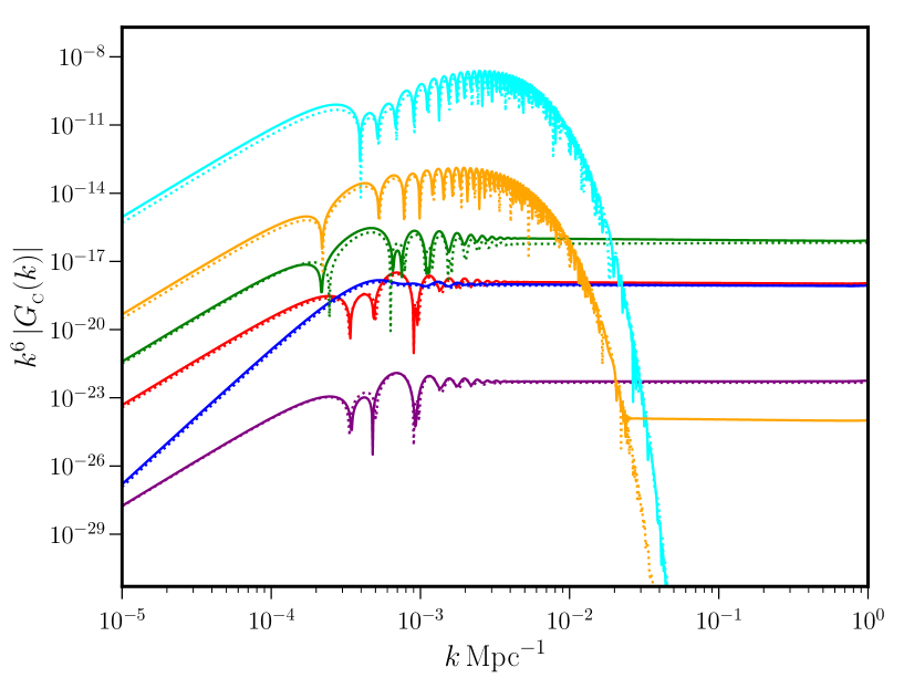
It is clear that the analytical results match well with the numerical results indicating the extent of accuracy of the numerical procedures we have adopted. As in the cases of QP and SMI, we find that the boundary terms, in particular $G_{8}(k)$, dominate at suitably small wave numbers.

V Amplitude and shape of the non-Gaussianity parameter

Having obtained the scalar bispectrum, let us now turn to understand the amplitude and shape of the corresponding non-Gaussianity parameter $f_{{}_{\mathrm{NL}}}$. In the next section, we shall discuss the behavior of the parameter in the so-called squeezed limit wherein it is expected to be expressed completely in terms of the scalar spectral index. In this section, we shall discuss the behavior in the equilateral limit as well as the complete shape, which is often illustrated in the form of density plots.

Let us first consider the equilateral limit. In Fig. 8, we have illustrated the behavior of the parameter $f_{{}_{\mathrm{NL}}}$ in the equilateral limit in the different models of our interest.

Figure 8: The scalar non-Gaussianity parameter $f_{{}_{\mathrm{NL}}}$ computed in the equilateral limit has been plotted for all the models of our interest: PI and SMII (in the top and bottom panels on the left), QPa, QPb and QPc (in the top three panels on the right, respectively, as red curves), SMIa, SMIb and SMIc (in the top three panels on the right, in blue) and, lastly, HCO (in the bottom panel on the right). Note that the scalar power spectrum appears in the denominator in the definition of $f_{{}_{\mathrm{NL}}}$ [cf. Eq. (24)]. The spike in the amplitude of $f_{{}_{\mathrm{NL}}}$ in the case of PI (at the left extreme of the figure) arises due to the sharp drop in the power spectrum (in this context, see Fig. 3). The oscillations with increasing amplitude at larger wave numbers in the case of SMII is caused due to the contribution from $G_{4}(k)+G_{7}(k)$, which rises linearly before eventually dying down (cf. Fig. 6). Such a behavior occurs due to the sharp transition that occurs in the evolution of the field as it crosses the discontinuity in the derivative of the potential. Also note that the maximum amplitude of $f_{{}_{\mathrm{NL}}}$ is larger in QPa and SMIa when compared to QPb and SMIb (also see Ref. [27]). This can be partly attributed to the larger initial velocity of the background scalar field when the initial conditions are imposed on the perturbations. Moreover, interestingly, we find that the amplitude of $f_{{}_{\mathrm{NL}}}$ is larger in the case of QP than SMI. Lastly, the amplitude of $f_{{}_{\mathrm{NL}}}$ in the cases of QPc, SMIc and HCO are extremely large, indicating that these models are unlikely to be viable in the light of the constraints on $f_{{}_{\mathrm{NL}}}$ from Planck.

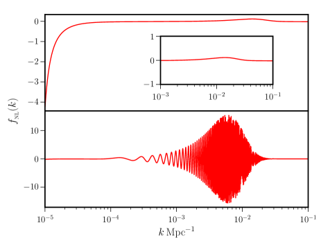
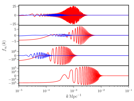
Recall that, according to the most recent constraints from Planck: $f_{{}_{\mathrm{NL}}}^{\rm local}=-0.9\pm 5.1$, $f_{{}_{\mathrm{NL}}}^{\rm equil}=-26\pm 47$ and $f_{{}_{\mathrm{NL}}}^{\rm ortho}=-38\pm 24$ [61]. Among the models we have considered, we find that the parameter $f_{{}_{\mathrm{NL}}}$ is very large in the cases of QPc, SMIc and HCO. In fact, these scenarios are likely to be inconsistent with the most recent constraints on the parameter. The models SMII and PI also lead to relatively large value of $f_{{}_{\mathrm{NL}}}$, but this can attributed to the sharp drop in the scalar power spectra over the relevant scales rather than a rise in the amplitude of the bispectrum. As we shall discuss in the concluding section, it seems urgent to arrive at a template for the bispectrum in models such as PI in order to be able to compare it with the CMB data at the level of three-point functions.

In Fig. 9, we have illustrated the complete shape of the scalar non-Gaussianity parameter $f_{{}_{\mathrm{NL}}}({\bm{k}}_{1},{\bm{k}}_{2},{\bm{k}}_{3})$ that arises in the various models of our interest in the form of density plots, as is usually done.

Figure 9: The amplitude and shape of the non-Gaussianity parameter $f_{{}_{\mathrm{NL}}}({\bm{k}}_{1},{\bm{k}}_{2},{\bm{k}}_{3})$ has been illustrated as density plots for the various models of our interest (QPa, SMIa and SMII from top to bottom on the left, and QPb, SMIb and PI in the same order on the right) as a function of $k_{1}/k_{3}$ and $k_{2}/k_{3}$. We have chosen $k_{3}$ to be the pivot scale in all the plots. Note that the top right and left corners of the triangles correspond to the non-Gaussianity parameter in the equilateral and squeezed limits, evaluated at the pivot scale, respectively.

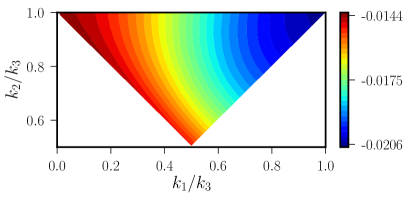
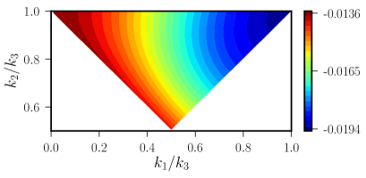
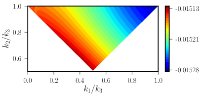
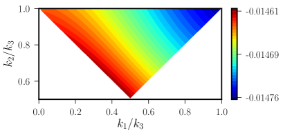
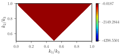
We should mention that the density plots of $f_{{}_{\mathrm{NL}}}$ have been computed with $k_{3}$ set to be the pivot scale (recall that, $k_{\ast}=0.05\,\mathrm{Mpc}^{-1}$). For the models QPa and QPb, we find that the non-Gaussianity parameter around the pivot scale is equilateral in shape corresponding to the slow roll value of $f_{{}_{\mathrm{NL}}}\simeq 2\times 10^{-2}$ in the equilateral limit (i.e. when $k_{1}=k_{2}=k_{3}$, corresponding to the top right corner of the triangular density plots). These results should be compared with the corresponding values in Fig. 8 around the pivot scale. The suppression in the scalar power spectrum, which occurs at roughly two decades away in wave number, does not affect the shape of $f_{{}_{\mathrm{NL}}}$ around the pivot scale. In the cases of SMIa and SMIb, we see a roughly similar behavior with a slightly lesser amplitude of $f_{{}_{\mathrm{NL}}}$ as expected in SMI models. In the case of SMII, we see small but persistent oscillations, with $f_{{}_{\mathrm{NL}}}\simeq 10^{-2}$, throughout the range of wave numbers around pivot scale. This can be understood from the behavior of the contribution $G_{4}(k)+G_{7}(k)$ in the model. In PI, the bispectrum is largely local in shape with a sharp increase in amplitude occurring at wave numbers around the location where the scalar spectrum exhibits a sharp drop in power.

VI Validity of the consistency relation

Let us now turn to the behavior of the three-point functions in the squeezed limit wherein one of the three wave numbers is much smaller than the other two [55, 62, 63, 58]. Since the amplitude of the long wavelength mode freezes on super-Hubble scales during inflation, it can be treated as part of the background. Consequently, one finds that, in such a limit, the three-point functions generated during inflation can be expressed entirely in terms of the two-point functions through the so-called consistency relation. In the squeezed limit, the scalar bispectrum is expected to reduce to the following form (see, for instance, Ref. [58]):

$$\lim_{k_{1}\to 0}G({\bm{k}}_{1},{\bm{k}},-{\bm{k}})=-\frac{(2\,\pi)^{4}}{4\,k_{1}^{3}\,k^{3}}\,\left[n_{{}_{\mathrm{S}}}(k)-1\right]\,{\mathcal{P}}_{{}_{\mathrm{S}}}(k_{1})\,{\mathcal{P}}_{{}_{\mathrm{S}}}(k),$$ (26)

where $n_{{}_{\mathrm{S}}}(k)=1+\left[{\mathrm{d}}\,{\rm ln}\,{\mathcal{P}}_{{}_{\mathrm{S}}}(k)/{\mathrm{d}}\,{\rm ln}\,k\right]$ is the scalar spectral index, and it should be clear that we have considered ${\bm{{\bm{k}}_{1}}}$ to be the squeezed mode. Upon substituting the above expression in the definition (24) for the non-Gaussianity parameter $f_{{}_{\mathrm{NL}}}({\bm{k}}_{1},{\bm{k}}_{2},{\bm{k}}_{3})$, we find that we can express the consistency relation in the squeezed limit as follows:

$$\lim_{k_{1}\to 0}\,f_{{}_{\mathrm{NL}}}({\bm{k}}_{1},{\bm{k}},-{\bm{k}})=\frac{5}{12}\,\left[n_{{}_{\mathrm{S}}}(k)-1\right]\equiv f_{{}_{\mathrm{NL}}}^{{}_{\rm CR}}(k).$$ (27)

With the results we have obtained, it is straightforward to examine if the consistency relation is satisfied in the models of our interest. Actually, it has already been established that the consistency relation is satisfied in SMII and PI despite the strong departures from slow roll, as reflected in the sharp features in the power spectra and bispectra (see Fig. 10; in this context, also see Refs. [43, 58]).

Figure 10: The non-Gaussianity parameter $f_{{}_{\mathrm{NL}}}(k)$ in the squeezed limit has been plotted (in red) for the cases of PI, SMII (top and bottom panels, on the left), QPa, QPb, SMIa and SMIb (panels from top to bottom in that order, on the right). We have also plotted the quantity $f_{{}_{\mathrm{NL}}}^{{}_{\rm CR}}(k)$ [cf. Eq. (27)], determined completely by the scalar spectral index, for each of these models (as dotted blue curves). Clearly, the consistency condition (27) is satisfied in PI and SMII (as is evident from the figure on the left) even over wave numbers wherein there arise strong departures from near scale invariance in the power and bi-spectra. In complete contrast, in QPa, QPb, SMIa and SMIb, the consistency condition is violated at large scales (as should be clear from the figure on the right), but it is eventually restored at the small scales (in this context, also see our earlier work [27]). We find that the behavior of $f_{{}_{\mathrm{NL}}}$ is similar in the cases of QPc, SMIc and HCO. Hence, we have not plotted them here. The difference arises only in the magnitude of $f_{{}_{\mathrm{NL}}}$ over large scales where the consistency condition is violated.

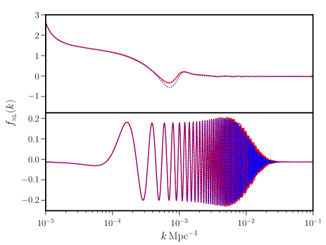
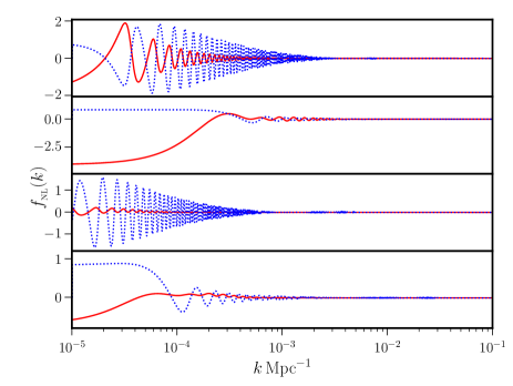
However, in the case of the scenarios with kinetically dominated initial conditions, we find that the consistency condition is violated on large scales where the scalar power spectrum exhibits a suppression. This should be clear from Fig. 10 wherein we have plotted the non-Gaussianity parameter $f_{{}_{\mathrm{NL}}}(k)$ in the squeezed limit as well as the quantity $f_{{}_{\mathrm{NL}}}^{{}_{\rm CR}}(k)$ [cf. Eq. (27)] for most of the models we have been interested in. We find that the consistency relation begins to be satisfied in these cases only at small scales (for $k\gtrsim 8\times 10^{-3}\,{\rm Mpc}^{-1}$) which emerge from sufficiently deep inside the Hubble radius [say, from $k\simeq 10^{2}\,\sqrt{|z^{\prime\prime}/z}|$] after slow roll inflation has set in. Evidently, the violation of the consistency condition is associated with the fact that the Bunch-Davies initial condition on the large scale modes are imposed when they are outside the Hubble radius. We should mention here that the violation of the consistency condition at large scales that we encounter is partly similar to the violation of the condition noticed earlier in the case of non-attractor inflation [64, 65, 66, 47, 48].

VII Summary and scope

At the level of the power spectrum, all the models we have considered here, viz. models with kinetically dominated initial conditions, their dual, the hard cut-off model, the second Starobinsky model and punctuated inflation, lead to a suppression of power on large scales. Naively, one would have expected that non-Gaussianities would help us discriminate between the different models, and we find that indeed they do. Though there arise some differences in the overall amplitude of the scalar bispectra in the various models, the crucial distinction seems to be their behavior in the squeezed limit. While the consistency condition is satisfied in PI and SMII over all the modes of cosmological interest, in the models with initial kinetic domination, their dual and HCO, the consistency relation is found to be violated on large scales for the modes that always remain in the super-Hubble regime. However, as in the cases of PI and SMII, in QP, SMI and HCO, the consistency relation is satisfied for the small scales modes which evolve from the sub-Hubble regime.

Models such as punctuated inflation or the second Starobinsky model may be considered to be more appealing theoretically than the models with kinetically dominated initial conditions. However, the data can help us evaluate the performance of the models and rule in favor of one over the other. In order to compare with the CMB data at the level of the bispectrum, it will be useful to obtain an analytical template for the scalar bispectrum (in this context, see, for example, Refs. [67, 68]). While there have been efforts to reproduce the power spectra analytically in the case of models with kinetically dominated initial conditions (in this context, see Ref. [7]), these analytical calculations seem to underestimate the amplitude of the oscillations that arise as the spectrum turns scale invariant. In the context of PI, there seems to have been no effort at all to arrive at the power spectrum analytically. We are currently working on evaluating the spectra as well as the bispectra analytically in PI as well as in models with kinetically dominated initial conditions with the aim of eventually comparing these models with the CMB data at the level of bispectra [69].

Appendix A Signatures of initial kinetic domination across models

To illustrate that the imprints of initial kinetic domination arise across all inflationary modes, in this appendix, we shall consider two other models of inflation, viz. a small field model and so-called the axion monodromy model, which are described by the following potentials:

$$V(\phi) = V_{0}\,\left[1-\left(\frac{\phi}{\phi_{0}}\right)^{4}\right],$$ (28a)

$$V(\phi) = \mu^{3}\,\left[\phi+b\,\phi_{0}\,{\rm cos}\,\left(\frac{\phi}{\phi_{0}}\right)\right].$$ (28b)

We work with parameters and initial conditions for the background such that the power spectra are COBE normalized around the pivot scale and the suppression on large scales occurs as in QPa. The corresponding scalar power spectra are illustrated in Fig. 11, and it is clear that, despite the different choice of potentials, the power spectra have the same shape at large and small scales across models.

Figure 11: The scalar power spectra in a small field inflationary model (in blue) and the axion monodromy model (in green) with kinetically dominated initial conditions have been plotted along with the power spectrum in the case of QPa (in red). The parameters have been chosen so that the features of the power spectra match at large scales. We should clarify we have not carried out a comparison of the small field model and the axion monodromy model against the CMB data.

In Fig. 12, we have plotted the behavior of the non-Gaussianity parameter $f_{{}_{\mathrm{NL}}}$ in the squeezed limit in these cases.

Figure 12: The behavior of the scalar non-Gaussianity parameter $f_{{}_{\mathrm{NL}}}$ in the squeezed limit has been plotted (in red) for the small field inflationary model (on top) and the axion monodromy model (at the bottom). Just as we had done earlier, we have also plotted the quantity $f_{{}_{\mathrm{NL}}}^{{}_{\rm CR}}$ (in blue). As in the cases of QP and SMI, while the consistency condition is violated at large scales, it is restored at small scales. This is clearly evident in the case of the axion monodromy model which is known to exhibit oscillations in the power spectrum as well as bispectrum even at small scales.

Clearly, the behavior of the parameter is similar to that encountered in the cases of QP and SMI. The restoration of the consistency condition is well illustrated in the case of the axion monodromy model, wherein both the power and bispectra exhibit continued oscillations even at small scales [70, 58].

Appendix B Constraints on the cosmological parameters

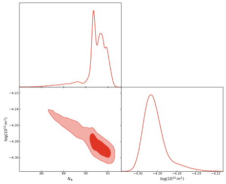
In this appendix, we shall present the confidence contours arrived at upon comparing the inflationary models of our interest with the CMB data. We shall focus on the three models SMIc, SMII and PI, which moderately improve the fit to the data [cf. Tab. 3]. We find that the background cosmological parameters, viz. $\Omega_{\mathrm{b}}h^{2}$, $\Omega_{\mathrm{c}}\,h^{2}$, $\theta$ and $\tau$ are constrained around the same region in the parameter space in cases of PL, SMIc and SMII. In case of PI, the contours differ slightly. However, we find that the distributions are within 1-$\sigma$ intervals of each other. In Fig. 13, we have illustrated the confidence contours for the inflationary parameters in the cases of SMIc and PI, models which are described by the parameters $\Lambda$ and $m$, apart from $N_{\ast}$.

Figure 13: We have presented the contours of the marginalized posterior distribution (1-$\sigma$ regions in dark red and 2-$\sigma$ regions in light red) of the inflationary parameters $\Lambda$ or $m$ and $N_{\ast}$ in the models of SMIc (on the left) and PI (on the right).

In Fig. 14, we have illustrated the constraints on all the inflationary parameters in the model SMII. In the figure, we have also included the constraints on the inflationary parameters in the PL case with a scale invariant tensor amplitude.

Figure 14: We have illustrated the contours of the marginalized posterior distribution of the parameters of the model SMII (in red) against the contours of the common parameters in the PL case (in blue), with a scale invariant tensor amplitude assumed in both the cases. Note that the contours on the parameters $A_{{}_{\mathrm{S}}}$, $n_{{}_{\mathrm{S}}}$ and $r$ overlap considerably in the two cases.

Lastly, in Fig. 15, we have presented the marginalized posterior distributions on the Hubble parameter $H_{0}$, which is of considerable interest today (in this context, see, for instance, the recent reviews [53, 54]).

Figure 15: We have presented the marginalized posterior distribution of the Hubble parameter $H_{0}$ arising in the PL case (in black) as well as in the inflationary models SMIc, SMII and PI (in red, blue and green). It is clear that that the estimates of $H_{0}$ from SMIc and SMII match that of the PL case. Whereas, the estimate from PI is slightly lower, which will actually aggravate the so-called Hubble tension.

We find that, while the mean values of $H_{0}$ in the cases of SMII and SMIc roughly match the value in the standard PL case, the mean value is lower in the case of PI which will aggravate the $H_{0}$ tension.

References

- Bridle et al. [2003] S. L. Bridle, A. M. Lewis, J. Weller, and G. Efstathiou, Mon. Not. Roy. Astron. Soc. 342, L72 (2003), arXiv:astro-ph/0302306 [astro-ph] .
- Shafieloo and Souradeep [2004] A. Shafieloo and T. Souradeep, Phys. Rev. D70, 043523 (2004), arXiv:astro-ph/0312174 [astro-ph] .
- Hunt and Sarkar [2004] P. Hunt and S. Sarkar, Phys. Rev. D70, 103518 (2004), arXiv:astro-ph/0408138 [astro-ph] .
- Hunt and Sarkar [2007] P. Hunt and S. Sarkar, Phys. Rev. D76, 123504 (2007), arXiv:0706.2443 [astro-ph] .
- Hazra et al. [2013a] D. K. Hazra, A. Shafieloo, and G. F. Smoot, JCAP 1312, 035, arXiv:1310.3038 [astro-ph.CO] .
- Cline et al. [2003] J. M. Cline, P. Crotty, and J. Lesgourgues, JCAP 0309, 010, arXiv:astro-ph/0304558 [astro-ph] .
- Contaldi et al. [2003] C. R. Contaldi, M. Peloso, L. Kofman, and A. D. Linde, JCAP 0307, 002, arXiv:astro-ph/0303636 [astro-ph] .
- Sinha and Souradeep [2006] R. Sinha and T. Souradeep, Phys. Rev. D74, 043518 (2006), arXiv:astro-ph/0511808 [astro-ph] .
- Powell and Kinney [2007] B. A. Powell and W. H. Kinney, Phys. Rev. D76, 063512 (2007), arXiv:astro-ph/0612006 [astro-ph] .
- Boyanovsky et al. [2006a] D. Boyanovsky, H. J. de Vega, and N. G. Sanchez, Phys. Rev. D74, 123007 (2006a), arXiv:astro-ph/0607487 [astro-ph] .
- Boyanovsky et al. [2006b] D. Boyanovsky, H. J. de Vega, and N. G. Sanchez, Phys. Rev. D74, 123006 (2006b), arXiv:astro-ph/0607508 [astro-ph] .
- Nicholson and Contaldi [2008] G. Nicholson and C. R. Contaldi, JCAP 0801, 002, arXiv:astro-ph/0701783 [astro-ph] .
- Jain et al. [2007] R. K. Jain, P. Chingangbam, and L. Sriramkumar, JCAP 0710, 003, arXiv:astro-ph/0703762 [astro-ph] .
- Jain et al. [2009] R. K. Jain, P. Chingangbam, J.-O. Gong, L. Sriramkumar, and T. Souradeep, JCAP 0901, 009, arXiv:0809.3915 [astro-ph] .
- Jain et al. [2010] R. K. Jain, P. Chingangbam, L. Sriramkumar, and T. Souradeep, Phys. Rev. D82, 023509 (2010), arXiv:0904.2518 [astro-ph.CO] .
- Hazra et al. [2014a] D. K. Hazra, A. Shafieloo, G. F. Smoot, and A. A. Starobinsky, Phys. Rev. Lett. 113, 071301 (2014a), arXiv:1404.0360 [astro-ph.CO] .
- Hazra et al. [2014b] D. K. Hazra, A. Shafieloo, G. F. Smoot, and A. A. Starobinsky, JCAP 1408, 048, arXiv:1405.2012 [astro-ph.CO] .
- White et al. [2014] J. White, Y.-l. Zhang, and M. Sasaki, Phys. Rev. D 90, 083517 (2014), arXiv:1407.5816 [astro-ph.CO] .
- Qureshi et al. [2017] M. H. Qureshi, A. Iqbal, M. A. Malik, and T. Souradeep, JCAP 1704, 013, arXiv:1610.05776 [astro-ph.CO] .
- Pi et al. [2018] S. Pi, Y.-l. Zhang, Q.-G. Huang, and M. Sasaki, JCAP 05, 042, arXiv:1712.09896 [astro-ph.CO] .
- Ramirez and Schwarz [2012] E. Ramirez and D. J. Schwarz, Phys. Rev. D85, 103516 (2012), arXiv:1111.7131 [astro-ph.CO] .
- Ramirez [2012] E. Ramirez, Phys. Rev. D85, 103517 (2012), arXiv:1202.0698 [astro-ph.CO] .
- Cicoli et al. [2014] M. Cicoli, S. Downes, B. Dutta, F. G. Pedro, and A. Westphal, JCAP 12, 030, arXiv:1407.1048 [hep-th] .
- Hergt et al. [2018a] L. T. Hergt, W. J. Handley, M. P. Hobson, and A. N. Lasenby, (2018a), arXiv:1809.07185 [astro-ph.CO] .
- Hergt et al. [2018b] L. T. Hergt, W. J. Handley, M. P. Hobson, and A. N. Lasenby, (2018b), arXiv:1809.07737 [astro-ph.CO] .
- Starobinsky [1992] A. A. Starobinsky, JETP Lett. 55, 489 (1992), [Pisma Zh. Eksp. Teor. Fiz.55,477(1992)].
- Ragavendra et al. [2020] H. Ragavendra, D. Chowdhury, and L. Sriramkumar, Springer Proc. Phys. 248, 39 (2020), arXiv:1906.03942 [astro-ph.CO] .
- Mukhanov et al. [1992] V. F. Mukhanov, H. A. Feldman, and R. H. Brandenberger, Phys. Rept. 215, 203 (1992).
- Martin [2004] J. Martin, Particles and fields. Proceedings, 24th National Meeting, ENFPC 24, Caxambu, Brazil, September 30-October 4, 2003, Braz. J. Phys. 34, 1307 (2004), arXiv:astro-ph/0312492 [astro-ph] .
- Martin [2005] J. Martin, Planck scale effects in astrophysics and cosmology. Proceedings, 40th Karpacs Winter School, Ladek Zdroj, Poland, February 4-14, 2004, Lect. Notes Phys. 669, 199 (2005), arXiv:hep-th/0406011 [hep-th] .
- Bassett et al. [2006] B. A. Bassett, S. Tsujikawa, and D. Wands, Rev. Mod. Phys. 78, 537 (2006).
- Sriramkumar [2009] L. Sriramkumar, (2009), arXiv:0904.4584 [astro-ph.CO] .
- Sriramkumar [2012] L. Sriramkumar, in Vignettes in Gravitation and Cosmology, edited by L. Sriramkumar and T. Seshadri (World Scientific, Singapore, 2012) pp. 207–249.
- Baumann [2011] D. Baumann, in Physics of the large and the small, TASI 09, proceedings of the Theoretical Advanced Study Institute in Elementary Particle Physics, Boulder, Colorado, USA, 1-26 June 2009 (2011) pp. 523–686, arXiv:0907.5424 [hep-th] .
- Linde [2015] A. Linde, in Proceedings, 100th Les Houches Summer School: Post-Planck Cosmology: Les Houches, France, July 8 - August 2, 2013 (2015) pp. 231–316, arXiv:1402.0526 [hep-th] .
- Martin [2016] J. Martin, The Cosmic Microwave Background, Astrophys. Space Sci. Proc. 45, 41 (2016), arXiv:1502.05733 [astro-ph.CO] .
- Chen et al. [2008] X. Chen, R. Easther, and E. A. Lim, JCAP 0804, 010, arXiv:0801.3295 [astro-ph] .
- Hazra et al. [2013b] D. K. Hazra, L. Sriramkumar, and J. Martin, JCAP 1305, 026, arXiv:1201.0926 [astro-ph.CO] .
- Horner and Contaldi [2013] J. S. Horner and C. R. Contaldi, (2013), arXiv:1303.2119 [astro-ph.CO] .
- Handley et al. [2014] W. J. Handley, S. D. Brechet, A. N. Lasenby, and M. P. Hobson, Phys. Rev. D89, 063505 (2014), arXiv:1401.2253 [astro-ph.CO] .
- Horner and Contaldi [2014] J. S. Horner and C. R. Contaldi, (2014), arXiv:1407.6948 [astro-ph.CO] .
- Arroja and Sasaki [2012] F. Arroja and M. Sasaki, JCAP 1208, 012, arXiv:1204.6489 [astro-ph.CO] .
- Martin and Sriramkumar [2012] J. Martin and L. Sriramkumar, JCAP 1201, 008, arXiv:1109.5838 [astro-ph.CO] .
- Martin et al. [2014] J. Martin, L. Sriramkumar, and D. K. Hazra, JCAP 1409 (09), 039, arXiv:1404.6093 [astro-ph.CO] .
- Dodelson and Hui [2003] S. Dodelson and L. Hui, Phys. Rev. Lett. 91, 131301 (2003), arXiv:astro-ph/0305113 [astro-ph] .
- Liddle and Leach [2003] A. R. Liddle and S. M. Leach, Phys. Rev. D68, 103503 (2003), arXiv:astro-ph/0305263 [astro-ph] .
- Cai et al. [2016] Y.-F. Cai, J.-O. Gong, D.-G. Wang, and Z. Wang, JCAP 10, 017, arXiv:1607.07872 [astro-ph.CO] .
- Cai et al. [2018] Y.-F. Cai, X. Chen, M. H. Namjoo, M. Sasaki, D.-G. Wang, and Z. Wang, JCAP 1805, 012, arXiv:1712.09998 [astro-ph.CO] .
- Aghanim et al. [2020a] N. Aghanim et al. (Planck), Astron. Astrophys. 641, A5 (2020a), arXiv:1907.12875 [astro-ph.CO] .
- Lewis et al. [2000] A. Lewis, A. Challinor, and A. Lasenby, Astrophys. J. 538, 473 (2000), arXiv:astro-ph/9911177 .
- Lewis and Bridle [2002] A. Lewis and S. Bridle, Phys. Rev. D 66, 103511 (2002), arXiv:astro-ph/0205436 .
- Aghanim et al. [2020b] N. Aghanim et al. (Planck), Astron. Astrophys. 641, A6 (2020b), arXiv:1807.06209 [astro-ph.CO] .
- Di Valentino et al. [2021] E. Di Valentino, O. Mena, S. Pan, L. Visinelli, W. Yang, A. Melchiorri, D. F. Mota, A. G. Riess, and J. Silk, Class. Quant. Grav. 38, 153001 (2021), arXiv:2103.01183 [astro-ph.CO] .
- Freedman [2021] W. L. Freedman, Astrophys. J. 919, 16 (2021), arXiv:2106.15656 [astro-ph.CO] .
- Maldacena [2003] J. M. Maldacena, JHEP 05, 013, arXiv:astro-ph/0210603 [astro-ph] .
- Seery and Lidsey [2005] D. Seery and J. E. Lidsey, JCAP 0506, 003, arXiv:astro-ph/0503692 [astro-ph] .
- Arroja and Tanaka [2011] F. Arroja and T. Tanaka, JCAP 1105, 005, arXiv:1103.1102 [astro-ph.CO] .
- Sreenath et al. [2015] V. Sreenath, D. K. Hazra, and L. Sriramkumar, JCAP 1502 (02), 029, arXiv:1410.0252 [astro-ph.CO] .
- Sreenath et al. [2013] V. Sreenath, R. Tibrewala, and L. Sriramkumar, JCAP 1312, 037, arXiv:1309.7169 [astro-ph.CO] .
- Sreenath and Sriramkumar [2014] V. Sreenath and L. Sriramkumar, JCAP 1410 (10), 021, arXiv:1406.1609 [astro-ph.CO] .
- Akrami et al. [2019] Y. Akrami et al. (Planck), (2019), arXiv:1905.05697 [astro-ph.CO] .
- Creminelli and Zaldarriaga [2004] P. Creminelli and M. Zaldarriaga, JCAP 0410, 006, arXiv:astro-ph/0407059 [astro-ph] .
- Cheung et al. [2008] C. Cheung, A. L. Fitzpatrick, J. Kaplan, and L. Senatore, JCAP 0802, 021, arXiv:0709.0295 [hep-th] .
- Namjoo et al. [2013] M. H. Namjoo, H. Firouzjahi, and M. Sasaki, EPL 101, 39001 (2013), arXiv:1210.3692 [astro-ph.CO] .
- Martin et al. [2013] J. Martin, H. Motohashi, and T. Suyama, Phys. Rev. D 87, 023514 (2013), arXiv:1211.0083 [astro-ph.CO] .
- Chen et al. [2013] X. Chen, H. Firouzjahi, M. H. Namjoo, and M. Sasaki, EPL 102, 59001 (2013), arXiv:1301.5699 [hep-th] .
- Adshead et al. [2011] P. Adshead, W. Hu, C. Dvorkin, and H. V. Peiris, Phys. Rev. D84, 043519 (2011), arXiv:1102.3435 [astro-ph.CO] .
- Basu et al. [2019] S. Basu, D. J. Brooker, N. C. Tsamis, and R. P. Woodard, Phys. Rev. D100, 063525 (2019), arXiv:1905.12140 [gr-qc] .
- Sohn and Fergusson [2019] W. Sohn and J. Fergusson, Phys. Rev. D100, 063536 (2019), arXiv:1902.01142 [astro-ph.CO] .
- Aich et al. [2013] M. Aich, D. K. Hazra, L. Sriramkumar, and T. Souradeep, Phys. Rev. D87, 083526 (2013), arXiv:1106.2798 [astro-ph.CO] .