Electronic structure of semiconductor nanoparticles from stochastic evaluation of imaginary-time path integral

Abstract

In the Kohn-Sham orbital basis imaginary-time path integral for electrons in a semiconductor nanoparticle has a mild Fermion sign problem and is amenable to evaluation by the standard stochastic methods. This is evidenced by the simulations of silicon hydrogen-passivated nanocrystals, such as $Si_{35}H_{36},~{}Si_{87}H_{76},~{}Si_{147}H_{100}$ and $Si_{293}H_{172},$ which contain $176$ to $1344$ valence electrons and range in size $1.0-2.4~{}nm$, utilizing the output of density functional theory simulations. We find that approximating Fermion action with just the leading order polarization term results in a positive-definite integrand in the functional integral, and that it is a good approximation of the full action. We compute imaginary-time electron propagators in these nanocrystals and extract the energies of low-lying electron and hole levels. Our quasiparticle gap predictions agree with the results of high-precision calculations using $G_{0}W_{0}$ technique. This formalism can be extended to calculations of more complex excited states, such as excitons and trions.

Applications of semiconductor nanomaterials require quantitative understanding of their electronic structure, including excited state properties. In recent years computational studies of atomistic models of these systems using ab initio electronic structure techniques have proven to be an attractive alternative to actual experiments as the ability to explore the vast set of possible configurations is inevitably limited. Currently, Density Functional Theory (DFT) Hohenberg and Kohn (1964); Kohn and Sham (1965) is the most useful first-principles atomistic tool for electronic structure. It combines reasonable accuracy and applicability, and naturally allows inclusion of surfaces, interfaces, dopants, ligands, etc.

However, DFT predicts ground state properties. Therefore, alternative methods are required to study the excited states. Currently, the most efficient comprehensive ab initio approach is based on many-body perturbation theory (MBPT), where DFT is augmented by the methods of perturbative many-body quantum mechanics. For instance, the GW method is used to compute single-particle energies, the Bethe-Salpeter equation (BSE) is solved for exciton states; an MBPT technique for three-body states, such as trions, has also been developed  Hedin (1965); Hybertsen and Louie (1986); Rohlfing and Louie (2000); Onida et al. (2002); Deilmann et al. (2016). The resulting energies and wave functions are subsequently used in calculations of various excited-state properties (e.g, Rohlfing and Louie (1998); Spataru et al. (2004); Kryjevski et al. (2018)).

Non-perturbative high-precision quantum Monte Carlo (QMC) techniques, such as fixed node, diffusion, and auxiliary field, exist (see, e.g., Zhang and Krakauer (2003); Austin et al. (2012); Zhang (2018)). Importantly, in these electronic systems the Fermion sign problem Schmidt and Kalos (1984); Loh et al. (1990) is mild enough to allow precise simulations. However, these MC methods are mostly suited for studying the ground state. Work to develop a QMC technique for excited states has started, but the studies so far have been based on the tight-binding approximation and applied to model systems (see, e.g., Zhang (1999); Rombouts et al. (1999)) and to graphene and carbon nanotubes Drut and Lähde (2009); Smith and von Smekal (2014); Ulybyshev et al. (2013); Otsuka et al. (2016); Beyl et al. (2018); Armour et al. (2011); Luu and Lähde (2016).

Here we present a DFT-based comprehensive nonperturbative QMC technique for a semiconductor nanoparticle, where excited states, such as electrons and holes, excitons and trions, can be obtained from the output of the same MC simulation. The system-specific Kohn-Sham (KS) orbitals are used as a basis in the electron action in the path integral representation of the statistical sum. Our results suggest that in this approach there is only a mild Fermion sign problem and evaluation by the standard stochastic importance sampling methods employed in, e.g., lattice Quantum Chromodynamics (QCD) (see Gattringer and Lang (2009) and references within) is possible. Specifically, we present results of simulations of several semiconductor nanocrystals, such as $Si_{35}H_{36},~{}Si_{87}H_{76},~{}Si_{147}H_{100}$ and $Si_{293}H_{172},$ including low-lying single-particle energies.

In the Born-Oppenheimer approximation the non-relativistic Hamiltonian for valence electrons is

$${\rm H} = \int{\rm d}{\bf x}~{}\psi^{\dagger}_{\alpha}\left(-\frac{\hbar^{2}\nabla^{2}}{2m}+eV_{eN}+A_{0}\right)\psi_{\alpha}+$$ (1)

$$+ \int\frac{{\rm d}{\bf x}}{8\pi e^{2}}\left({{\vec{\nabla}}A_{0}}\right)^{2}\ .$$ (2)

Here $\psi_{\alpha}({\bf x})$ is the electron field operator, $\alpha$ is the spin index, $e$ is the electron charge, $V_{eN}({\bf x},{\bf R}_{I})$ is a pseudopotential, i.e., an effective potential of ions at positions ${\bf R}_{I}$ felt by the valence electrons Phillips (1958); Yin and Cohen (1982); $A_{0}({\bf x})$ is the scalar potential operator which mediates electron electrostatic interactions. Note that the $A_{0}$ terms can be integrated out leading to the standard two-body Coulomb interaction operator.

The Kohn-Sham (KS) equation of the orbital-based DFT with a semi-local exchange-correlation functional, such as that by Perdew, Burke and Ernzerhof (PBE) Perdew et al. (1996), is

$$\left(-\frac{\hbar^{2}}{2m}\nabla^{2}+eV_{eN}+eV_{KS}\right)\phi_{i}({\bf x})=\epsilon_{i}\phi_{i}({\bf x}),$$ (3)

$$V_{KS}=V_{H}+V_{xc},~{}V_{H}({\bf x})=\int{\rm d}{\bf x}^{\prime}\frac{en({\bf x}^{\prime})}{|{\bf x}-{\bf x}^{\prime}|},$$ (4)

$$V_{xc}({\bf x})=\frac{\delta E_{xc}[n]}{e\delta n({\bf x})},\vspace{-1.2cm}$$ (5)

where $\phi_{i}({\bf x}),\epsilon_{i}$ are the KS orbitals and eigenvalues, respectively, and $E_{xc}[n]$ is the exchange-correlation functional, and $n({\bf x})$ is the ground state density of valence electrons Kohn and Sham (1965); Kümmel and Kronik (2008); Perdew et al. (1996). In general, the state label $i$ may include band number, lattice wave vector and spin label. But in this work we only consider spin-symmetric aperiodic systems so that $\phi_{i\uparrow}({\bf x})=\phi_{i\downarrow}({\bf x})\equiv\phi_{i}({\bf x})$. Extending this approach to the case of a periodic and/or spin-polarized system is straightforward.

In order to utilize electronic structure information from the DFT output we introduce ${\rm a}_{i\alpha},$ which is the annihilation operator of a Fermion in the KS state $|{i,\alpha}\rangle,$ so that $\psi_{\alpha}({\bf x})=\sum_{i}\phi_{i}({\bf x}){\rm a}_{i\alpha}$ (see, e.g., Abrikosov et al. (1963); Fetter and Walecka (1971)). In terms of ${\rm a}_{i\alpha}$ the imaginary-time (Euclidean) action corresponding to the Hamiltonian (2) is

$${S}_{E}=\int_{0}^{\beta}{\rm d}\tau\left(\sum_{ij\alpha}a^{\dagger}_{i\alpha}(\tau)\left[\left(\partial_{\tau}+\epsilon_{i}-\mu\right)\delta_{ij}-V^{xc}_{ij}+{\rm i}{A_{ij}}\right]a_{j\alpha}(\tau)-{\rm i}\int{\rm d}{\bf x}A_{0}n({\bf x})+\int\frac{{\rm d}{\bf x}}{8\pi e^{2}}\left({{\vec{\nabla}}A_{0}}\right)^{2}\right),$$ (6)

where $~{}\beta={1}/{T_{e}},~{}T_{e}$ is the electronic temperature in energy units used in the simulation, and

$$A_{ij}(\tau) = \int{\rm d}{\bf x}\phi^{*}_{i}({\bf x})A_{0}(\tau,{\bf x})\phi_{j}({\bf x}),$$ (7)

$$V^{xc}_{ij} = e\int{\rm d}{\bf x}\phi^{*}_{i}(\textrm{{x}})V^{xc}(\textrm{{x}})\phi_{j}(\textrm{{x}})\ .$$ (8)

The spatial integration is over the simulation box volume; KS indices $i$ and $j$ vary over the range of KS orbitals included in the simulation - the “active window”. Fermion fields $a_{i\alpha}(\tau)$ are anti-periodic $a_{i}(\tau)=-a_{i}(\tau+\beta),$ while the $A_{0}$-fields are periodic in time. The grand canonical chemical potential $\mu$ is set at the mid-gap which ensures charge neutrality. In order to obtain (6) we added and subtracted $eV_{KS}({\bf x})$ from (5) to the electron lagrangian, and then used ${\nabla}^{2}V_{H}=-4\pi en({\bf x})$ combined with the shift-invariance of the functional integration over $A_{0}.$ The statistical sum is given by

$$Z(\mu,T_{e})=\displaystyle\int{\rm D}A{\rm D}a_{i}{\rm D}a^{\dagger}_{i}\exp\left(-{S}_{E}\right).$$ (9)

The advantage of using KS orbital basis is that these states approximate binding of electrons to the ions and some of the electron interactions. Also, since KS states are labeled by their energy, it is straightforward to only include few KS states near the Fermi level that are relevant to the description of low-energy excitations, which is more efficient than using spatial grid covering the whole simulation cell. Thus, in this approach low-energy excitations of a nanoparticle are described by the KS quasiparticles subject to the static potential $V^{xc}_{ij}$ and interacting via $A_{ij}(\tau)$ exchanges. Strictly speaking, one should proceed using the basis of $\epsilon_{i}\delta_{ij}-V^{xc}_{ij}$ eigenstates. However, setting $V^{xc}_{ij}=V^{xc}_{ii}\delta_{ij}$ is an approximation often made in the GW method Onida et al. (2002); Govoni and Galli (2015). Also, for the systems we have simulated and for the range of KS states included, $V^{xc}_{ij}$ is strongly dominated by its diagonal entries. So, here we also approximate $V^{xc}_{ij}=V^{xc}_{ii}\delta_{ij}.$

Next we perform Grassmann integration over the Fermion variables and expand the resulting action ${S}(A_{0})$ in powers of $A_{0}(\tau,{\bf x}).$ The terms linear in $A_{0}$ cancel, which reflects the system’s overall charge neutrality. Retaining the leading non-vanishing term in the expansion yields the following action

$${S}_{2}=-\int\frac{{\rm d}\tau{\rm d}\textrm{{x}}}{8\pi e^{2}}A_{0}\nabla^{2}A_{0}-{\rm tr}{\cal M}{\cal A}{\cal M}{\cal A}+{\cal O}\left({A_{0}}^{3}\right),$$ (10)

where

$${\cal M}^{-1}_{ij}(\tau)=\left(\partial_{\tau}+\tilde{\epsilon}_{i}\right)\delta_{ij},~{}\tilde{\epsilon}_{i}=\epsilon_{i}-\mu-V^{xc}_{ii},$$ (11)

is the inverse non-interacting propagator and ${\cal A}_{i\tau,j\tau^{{}^{\prime}}}=A_{ij}(\tau)\delta_{\tau\tau^{{}^{\prime}}}.$ The second term in (10) includes the random phase approximation (RPA) polarization insertion in the KS orbital basis. The approximate action (10) has been used in this work to simulate the nanoparticle electrons. But, in order to evaluate the statistical sum (9) numerically we define the action on a discretized space-time grid. The Lagrangian corresponding to the Hamiltonian in (2) is invariant under time-dependent, spatially uniform $U(1)$ gauge transformations

$$\psi^{{}^{\prime}}(\tau)=e^{{\rm i}\Lambda(\tau)}\psi(\tau),~{}A_{0}^{{}^{\prime}}=A_{0}-\partial_{\tau}\Lambda(\tau),$$ (12)

where $\Lambda(\tau)$ is a function of time Drut and Lähde (2009). Note that the gauge field action - the last term in (6) - is invariant under (12) Drut and Lähde (2009) .

To generate $A_{0}$-field configurations we have used the frequency representation and a spatial grid, where the polarization term was expressed as a function of $\textrm{{x}},\textrm{{y}}$ using $\phi_{j}({\textrm{{x}}}).$ In this case $A_{0}(\omega,\textrm{{x}})$ can be used instead of the link variables required on a Euclidean time lattice Wilson (1974). However, a $\tau$-KS lattice, where ${\{}A_{0}(\omega,\textrm{{x}}){\}}$ have been converted to the link variables, has been used to compute the observables. While more computationally expensive than a $\tau$-KS lattice, the $\omega\textrm{{x}}$ basis is used since 1) numerical cancellation of the “tadpole” terms in a simulation requires perfect representation of the time derivative operator; 2) the Laplacian in the gauge field action cannot be represented accurately with the few KS orbitals included in a reasonably sized active window. Then, the action is

$${S}_{2}(A_{0})=-\sum_{k\geq 0}\sum_{\textrm{{x}},\textrm{{y}}}A_{0}^{*}(\omega_{k},\textrm{{x}}){\cal S}_{k}(\textrm{{x}},\textrm{{y}})A_{0}(\omega_{k},\textrm{{y}}),$$ (13)

where $\omega_{k}=2\pi kT_{e}$ is a bosonic Matsubara frequency, and

$${\cal S}_{k}(\textrm{{x}},\textrm{{y}}) = \frac{a_{x}a_{y}a_{z}T_{e}}{8\pi e^{2}}\nabla^{2}_{\textrm{{x}},\textrm{{y}}}+2(a_{x}a_{y}a_{z})^{2}\sum_{ij}\phi^{*}_{i}(\textrm{{x}})\phi_{j}({\textrm{{x}}})\phi^{*}_{j}(\textrm{{y}})\phi_{i}(\textrm{{y}})\frac{n_{j}-n_{i}}{2\pi{\rm i}k-\beta{\tilde{\epsilon}}_{j}+\beta{\tilde{\epsilon}}_{i}},$$ (14)

$$\nabla^{2}_{\textrm{{x}},\textrm{{y}}} = \sum_{l=1}^{3}\left(\nabla_{l}^{2}\right)_{\textrm{{x}},\textrm{{y}}},~{}\nabla_{l}^{2}f(\textrm{{x}})=\frac{1}{a_{l}^{2}}\left(f\left(\textrm{{x}}+a_{l}\hat{l}\right)-2f(\textrm{{x}})+f\left(\textrm{{x}}-a_{l}\hat{l}\right)\right)+{\cal O}(a_{l}^{2}),$$ (15)

where $a_{l},~{}l={x,y,z},$ are the lattice spacings and $n_{i}=\left({\rm exp}\left[\beta{\tilde{\epsilon}}_{i}\right]+1\right)^{-1}.$ Gauge invariance requires that each included $A(\omega)$ is coupled to at least one pair of fermion modes $a^{\dagger}(\omega_{1}),~{}a(\omega_{2})$ with $\omega=\omega_{2}-\omega_{1}.$ Therefore, in the simulations where a finite frequency cutoff was used the expression for ${\cal S}_{k}(\textrm{{x}},\textrm{{y}})$ was modified accordingly.

Importantly, ${\cal S}_{k}(\textrm{{x}},\textrm{{y}})$ from (15) is real and symmetric under $\textrm{{x}}\leftrightarrow\textrm{{y}},$ which is due to the basic properties of KS eigenfunctions (see, e.g., Landau and Lifshitz (1981)). Then the action ${S}_{2}(A_{0})$ from (13) is non-negative, which suggests that in this approach meaningful simulations are possible without resorting to sign-suppression techniques (see, e.g., Fodor and Katz (2002); Aarts (2009)). The size of neglected higher order terms in the action expansion will be discussed later.

The action (13) is quadratic in $A_{0}$. Therefore, importance sampling is done by diagonalizing ${\cal S}(\omega_{k},\textrm{{x}},\textrm{{y}})$ for each $\omega_{k}$ which results in

$${S}_{2}(A_{0})=\sum_{k\geq 0}\sum_{i=1}^{N_{x}-1}\frac{\lambda_{i}(\omega_{k})}{2}\left(u(\omega_{k})_{i}^{2}+{v}(\omega_{k})_{i}^{2}\right),$$ (16)

where $\lambda_{i}(\omega_{k})>0,{v}(0)_{i}\equiv 0,~{}N_{x}$ is the number of spatial grid points. Then one generates random values for the $u(\omega_{k})_{i},~{}{v}(\omega_{k})_{i}$ variables that are distributed normally according to the corresponding eigenvalue $\lambda_{i}(\omega_{k}),$ and changes the basis to get the $A_{0}(\tau,\textrm{{x}})$ configurations. For all the nanocrystals simulated here ${\cal N}\simeq 10^{3}$ configurations have been found to be sufficient to obtain statistically significant results.

The observables considered here are the electron and hole quasi-particle energies, which have been extracted from two-point propagators, which are the averages of the matrix elements of the propagator matrix corresponding to the state $i$ and time slices $\tau_{1}$ and $\tau_{2},$ in the long-time limit. For a particle state $i>HO,$ where $HO$ labels the highest occupied orbital, it is $E_{g}\beta\gg E_{g}\tau\gg 1,$ where $E_{g}$ is the quasiparticle gap. Then

$${\rm M}_{i}(A_{0})(\tau_{2},\tau_{1})=\left(\delta\left[{\rm D}+\tilde{\epsilon}_{i}\right]\right)^{-1}|_{i\tau_{2},i\tau_{1}},$$

$${\rm D}_{ij}f(\tau)=\frac{1}{\delta}\left(f(\tau+\delta)-e^{-{\rm i}\delta A_{ij}(\tau)}f(\tau)\right),$$

$${\rm M}_{i}(\tau,0)=\langle{{\rm M}_{i}(A_{0})}\rangle=\sum_{k=1}^{{\cal N}}\frac{{\rm M}_{i}(A^{k}_{0})}{\cal N}\rightarrow{}Ce^{-E_{i}\tau}\ ,$$ (17)

where $\delta=\beta/N_{t},~{}N_{t}$ is the number of time grid points, $A_{ij}(\tau)$ is defined in (8), $\tilde{\epsilon}_{i}$ is defined in (11). The last line in (17) shows the behavior of the correlator at large times on the fully interacting excitation energy $E_{i}$ ($C$ is an irrelevant coefficient). We fit for this energy and estimate the statistical error of $E_{i}$ via the bootstrapping technique Kunsch (1989). A full error analysis, which would include an assessment of systematic errors due to, e.g., fit-window sizes and fitting functions, finite lattice spacings, etc., is left to future work, though we do not expect the uncertainties quoted here to change significantly. We have used time grids with $\delta=0.025~{}eV^{-1}$ for all systems after checking that KS energies can be accurately extracted from the propagators in the non-interacting cases. Frequency cutoffs were chosen so that $\omega_{max}\delta\simeq 1.$ The procedure to extract hole excitation energies is analogous.

DFT simulations of the atomistic models of the nanocrystals (such as $Si_{293}H_{172}$ shown in Fig. 1), including geometry relaxation, have been done using Quantum Espresso DFT program with the PBE exchange-correlation functional Giannozzi et al. (2009). Norm-conserving pseudopotentials Hamann et al. (1979) have been used ensuring that the KS orbitals are orthonormal. Kinetic energy cutoff, which determines lattice spacings $a_{i},~{}i=x,y,z,$ has been set to $340.1~{}eV,$ which is the same as in Govoni and Galli (2015), resulting in $a_{i}\simeq 0.05~{}nm.$ Models of the nanocrystals ranging in size from $1.0$ to $2.4~{}nm$ were placed in the periodic cubic simulation boxes with about $1~{}nm$ of vacuum between the surfaces in order to prevent spurious interactions between periodic images. The number of KS orbitals included in the simulations have been chosen so that $\epsilon_{i_{max}}-\epsilon_{HO}\simeq\epsilon_{HO+1}-\epsilon_{i_{min}}\geq 1.5E^{PBE}_{g},$ where $i_{max},~{}i_{min}$ are the highest and the lowest included KS orbital labels and $E^{PBE}_{g}=\epsilon_{HO+1}-\epsilon_{HO}$ is the non-interacting gap. The corresponding number of states above/below Fermi level included in the simulation varied from 36 to 96 as the system’s size increased.

For the nanoparticles considered in this work $V^{xc}_{ii}$ shifts are sizable and tend to shrink the non-interacting gap $E^{PBE}_{g}$. This would require lowering $T_{e}$ in order to maintain $E^{PBE}_{g}\gg T_{e}$ required for the tadpole term cancellation, which would significantly increase the computational expense. So, here we have treated $V^{xc}_{ii}$ as self-energy corrections, i.e., we have simulated with $\tilde{\epsilon}_{i}=\epsilon_{i}-\mu$ and then subtracted $V^{xc}_{ii}$ from the resulting single-particle energies.

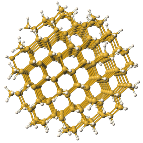
Figure 1: Atomistic model of $Si_{293}H_{172}.$ The smaller (white) surface atoms are the hydrogens.

$Si_{35}H_{36}$ $Si_{87}H_{76}$ $Si_{147}H_{100}$ $Si_{293}H_{172}$ $T_{e},~{}eV$ $0.5$ $0.5$ $0.4$ $0.3$ $N_{e}$ $176$ $424$ $688$ $1344$ $\langle{\tilde{s}}_{2}\rangle$ $74.1(5)$ $76.2(3)$ $315.4(3.4)$ $167.2(3)$ $Re\langle{s}\rangle$ $64.0(3)$ $70.0(2)$ $287.9(2.1)$ $162.2(2)$ $Im\langle{s}\rangle$ $0.1(2)$ $-0.1(1)$ $0.2(2)$ $-0.1(2)$ $\langle{\tilde{s}}_{2}/|{s}|\rangle$ $1.155(1)$ $1.0865(7)$ ${1.073(3)}$ ${1.0294(3)}$ $\langle{\rm tan}(\varphi)\rangle$ $0.002(3)$ $(-0.6\pm 2.0)\cdot 10^{-3}$ $0.0006(8)$ $-0.0005(12)$

Table 1: Both $s$ and ${\tilde{s}}_{2}$ dimensionless; ${s}=|s|e^{i\varphi}$. Numbers in parentheses represent statistical errors. $N_{e}$ is the valence electron number.

The calculation results are shown in Tables I and II. In order to check the size of the terms neglected in the approximate action (13) we used the A-configurations generated with (13) to compute

$${s} = {\rm tr}~{}{\rm log}\left(\frac{{\cal M}^{-1}+{\rm i}{\cal A}}{{\cal M}^{-1}}\right)-{\rm i}~{}{\rm tr}\left({\cal M}{\cal A}\right),$$ (18)

$${\tilde{s}}_{2} = \frac{1}{2}{\rm tr}\left({\cal M}{\cal A}{\cal M}{\cal A}\right).$$ (19)

While ${\tilde{s}}_{2}$ is only the leading non-vanishing term in the expansion of $s,$ we have found that in all cases $\langle{\tilde{s}}_{2}/|{s}|\rangle$ is close to one. (See Table I.) This suggests that the full Fermion action can be reasonably approximated by just the leading term. The average of the action’s phase $\varphi,$ where $s=|s|e^{i\varphi},$ is close to zero, which suggests that the sign problem in these systems is mild. Shown in Table II are the quasiparticle gap predictions in these nanocrystals. Our results agree with the results of high-precision calculations using $G_{0}W_{0}$ for the same nanocrystals Govoni and Galli (2015). Low-energy particle and hole levels in $Si_{293}H_{172}$ are shown in Fig. 2.

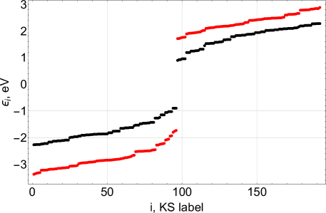
Figure 2: Interacting quasi-particle energies (red) for $Si_{293}H_{172}$. Black points are the KS eigenvalues. Error bars are too small to be seen at this scale.

$Si_{35}H_{36}$ $Si_{87}H_{76}$ $Si_{147}H_{100}$ $Si_{293}H_{172}$ $E_{g}^{PBE}$ 3.51 2.59 2.29 1.79 $E_{g}^{QP}$ $6.29(9)$ $4.76(8)$ $4.22(6)$ $3.45(3)$ $E_{g}^{G_{0}W_{0}}$ 6.29 4.77 4.21 3.46

Table 2: All entries are in eV. $E_{g}\equiv\epsilon_{HO+1}-\epsilon_{HO}$, is the PBE gap; the interacting gap is $E^{QP}_{g}=E_{p}^{min}-E_{h}^{max}.$ ${G_{0}W_{0}}$ results are from Govoni and Galli (2015).

In conclusion, we have performed initial steps toward development of a first-principles high-precision Monte Carlo technique for the excited states of a semiconductor nanoparticle, which utilizes KS orbital basis in the imaginary-time functional integral for the electrons. We find that approximating Fermion action with the leading order RPA polarization term in the expansion in powers of $A_{0}$ leads to a positive definite integrand in the statistical sum and that it is a reasonable approximation to the full action; $\langle{\tilde{s}}_{2}/|{s}|\rangle-1$ can be viewed as a source of systematic error. So, our results suggest that in this approach these systems have only a mild Fermion sign problem. Obvious improvements to our approximate calculations would be to use the full action instead of our quadratic approximation in (10), which could be done via re-weighting Salsburg et al. (1959); Ferrenberg and Swendsen (1988) or more advanced sampling techniques (e.g., hybrid Monte Carlo Duane et al. (1987)). Work to develop technique for other excited states, such as excitons and trions, is in progress.

The authors acknowledge use of computational resources at the Center for Computationally Assisted Science and Technology (CCAST) at North Dakota State University. TL acknowledges financial support from the Deutsche Forschungsgemeinschaft (Sino-German CRC 110). VVK acknowledges support by the Department of Energy National Nuclear Security Administration under Award No. DE-NA0003856.

References

- Hohenberg and Kohn (1964) P. Hohenberg and W. Kohn, Phys. Rev. 136, B864 (1964).
- Kohn and Sham (1965) W. Kohn and L. J. Sham, Phys. Rev. 140, A1133 (1965).
- Hedin (1965) L. Hedin, Phys. Rev. 139, A796 (1965).
- Hybertsen and Louie (1986) M. Hybertsen and S. Louie, Phys. Rev. B 34, 5390 (1986).
- Rohlfing and Louie (2000) M. Rohlfing and S. Louie, Phys. Rev. B 62, 4927 (2000).
- Onida et al. (2002) G. Onida, L. Reining, and A. Rubio, Rev. Mod. Phys. 74, 601 (2002).
- Deilmann et al. (2016) T. Deilmann, M. Drüppel, and M. Rohlfing, Phys. Rev. Lett. 116, 196804 (2016).
- Rohlfing and Louie (1998) M. Rohlfing and S. G. Louie, Phys. Rev. Lett. 80, 3320 (1998).
- Spataru et al. (2004) C. D. Spataru, S. Ismail-Beigi, L. X. Benedict, and S. G. Louie, Phys. Rev. Lett. 92, 077402 (2004).
- Kryjevski et al. (2018) A. Kryjevski, D. Mihaylov, and D. Kilin, The Journal of Physical Chemistry Letters 9, 5759 (2018).
- Zhang and Krakauer (2003) S. Zhang and H. Krakauer, Phys. Rev. Lett. 90, 136401 (2003).
- Austin et al. (2012) B. M. Austin, D. Y. Zubarev, and J. William A. Lester, Chemical Reviews 112, 263 (2012).
- Zhang (2018) S. Zhang, in Handbook of Materials Modeling, W. Andreoni, S. Yip (eds.) (Springer, Cham, 2018).
- Schmidt and Kalos (1984) K. E. Schmidt and M. H. Kalos, in Applications of theMonte Carlo Method in Statistical Physics, edited by K. Binder (Springer-Verlag, Heidelberg, 1984).
- Loh et al. (1990) E. Y. Loh, J. E. Gubernatis, R. T. Scalettar, S. R. White, D. J. Scalapino, and R. L. Sugar, Phys. Rev. B 41, 9301 (1990).
- Zhang (1999) S. Zhang, Phys. Rev. Lett. 83, 2777 (1999).
- Rombouts et al. (1999) S. M. A. Rombouts, K. Heyde, and N. Jachowicz, Phys. Rev. Lett. 82, 4155 (1999).
- Drut and Lähde (2009) J. E. Drut and T. A. Lähde, Phys. Rev. B 79, 165425 (2009).
- Smith and von Smekal (2014) D. Smith and L. von Smekal, Phys. Rev. B89, 195429 (2014), eprint 1403.3620.
- Ulybyshev et al. (2013) M. V. Ulybyshev, P. V. Buividovich, M. I. Katsnelson, and M. I. Polikarpov, Phys. Rev. Lett. 111, 056801 (2013).
- Otsuka et al. (2016) Y. Otsuka, S. Yunoki, and S. Sorella, Phys. Rev. X6, 011029 (2016), eprint 1510.08593.
- Beyl et al. (2018) S. Beyl, F. Goth, and F. F. Assaad, Phys. Rev. B97, 085144 (2018).
- Armour et al. (2011) W. Armour, S. Hands, and C. Strouthos, Phys. Rev. B 84, 075123 (2011).
- Luu and Lähde (2016) T. Luu and T. A. Lähde, Phys. Rev. B 93, 155106 (2016).
- Gattringer and Lang (2009) C. Gattringer and C. Lang, Quantum Chromodynamics on the Lattice: An Introductory Presentation, Lecture Notes in Physics (Springer Berlin Heidelberg, 2009).
- Phillips (1958) J. C. Phillips, Phys. Rev. 112, 685 (1958).
- Yin and Cohen (1982) M. T. Yin and M. L. Cohen, Phys. Rev. B 25, 7403 (1982).
- Perdew et al. (1996) J. P. Perdew, K. Burke, and M. Ernzerhof, Phys. Rev. Lett. 77, 3865 (1996).
- Kümmel and Kronik (2008) S. Kümmel and L. Kronik, Rev. Mod. Phys. 80, 3 (2008).
- Abrikosov et al. (1963) A. A. Abrikosov, L. Gorkov, and I. E. Dzyaloshinski, Methods of Quantum Field Theory in Statistical Physics (Prentice-Hall, Englewood Cliffs, NJ, 1963).
- Fetter and Walecka (1971) A. L. Fetter and J. Walecka, Quantum Theory of Many-Particle Systems (McGraw-Hill, New York, 1971).
- Govoni and Galli (2015) M. Govoni and G. Galli, Journal of Chemical Theory and Computation 11, 2680 (2015).
- Wilson (1974) K. G. Wilson, Phys. Rev. D 10, 2445 (1974).
- Landau and Lifshitz (1981) L. Landau and E. Lifshitz, Quantum Mechanics: Non-Relativistic Theory, Course of Theoretical Physics (Elsevier Science, 1981).
- Fodor and Katz (2002) Z. Fodor and S. D. Katz, Phys. Lett. B534, 87 (2002).
- Aarts (2009) G. Aarts, Phys. Rev. Lett. 102, 131601 (2009).
- Kunsch (1989) H. R. Kunsch, Ann. Statist. 17, 1217 (1989).
- Giannozzi et al. (2009) P. Giannozzi, S. Baroni, N. Bonini, M. Calandra, R. Car, C. Cavazzoni, D. Ceresoli, G. L. Chiarotti, M. Cococcioni, I. Dabo, et al., J. Phys.: Condensed Matter 21, 395502 (2009).
- Hamann et al. (1979) D. R. Hamann, M. Schlüter, and C. Chiang, Phys. Rev. Lett. 43, 1494 (1979).
- Salsburg et al. (1959) Z. W. Salsburg, J. D. Jacobson, W. Fickett, and W. W. Wood, The Journal of Chemical Physics 30, 65 (1959).
- Ferrenberg and Swendsen (1988) A. M. Ferrenberg and R. H. Swendsen, Phys. Rev. Lett. 61, 2635 (1988).
- Duane et al. (1987) S. Duane, A. D. Kennedy, B. J. Pendleton, and D. Roweth, Phys. Lett. B195, 216 (1987).