A census of the pulsar population observed with the international LOFAR station FR606 at low frequencies (25-80 MHz)

Abstract

Context. To date, only 69 pulsars have been identified with a detected pulsed radio emission below 100 MHz. A LOFAR-core LBA census and a dedicated campaign with the Nançay LOFAR station in stand-alone mode were carried out in the years 2014$-$2017 in order to extend the known population in this frequency range.

Aims. In this paper, we aim to extend the sample of known radio pulsars at low frequencies and to produce a catalogue in the frequency range of 25-80 MHz. This will allow future studies to probe the local Galactic pulsar population, in addition to helping explain their emission mechanism, better characterising the low-frequency turnover in their spectra, and obtaining new information about the interstellar medium through the study of dispersion, scattering, and scintillation.

Methods. We observed 102 pulsars that are known to emit radio pulses below 200 MHz and with declination above $-30\text{\,}\mathrm{\SIUnitSymbolDegree}$. We used the the Low Band Antennas (LBA) of the LOw Frequency ARray (LOFAR) international station FR606 at the Nançay Radio Observatory in stand-alone mode, recording data between 25-80 MHz.

Results. Out of our sample of 102 pulsars, we detected 64. We confirmed the existence of ten pulsars detected below 100 MHz by the LOFAR LBA census for the first time (Bilous et al., 2019) and we added two more pulsars that had never before been detected in this frequency range. We provided average pulse profiles, DM values, and mean flux densities (or upper limits in the case of non-detections). The comparison with previously published results allows us to identify a hitherto unknown spectral turnover for five pulsars, confirming the expectation that spectral turnovers are a widespread phenomenon.

1 Introduction

Until recently, radio frequencies below 100 MHz were largely under-explored in pulsar astronomy. The reasons for this are manifold: the interstellar medium causes high dispersion delays, which lead to pulse smearing unless coherent de-dispersion is used (computationally very expensive at such low frequencies); scattering on the inhomogeneities in the interstellar medium, leading to pulse smearing (regardless of the de-dispersion method); spectral turnover leading to low flux densities; the steep spectrum of the galactic background further reducing the measured signal-to-noise ratio (S/N); and the terrestrial ionosphere introducing angular shifts. Moreover, the times of arrival of pulsations extracted at such frequencies are highly affected by the profile frequency evolution due to the dependency of the emission altitude in the pulsar magnetosphere on the emission frequency (radius-to-frequency-mapping; see, e.g. Ruderman & Sutherland, 1975; Cordes, 1978).

However, these effects do not only pose problems for observations. They also constitute a treasure trove of rich and complex phenomena which can be studied with sufficiently sensitive radio telescopes. For example, following the radius-to-frequency-mapping, low-frequency radio emission traces the higher altitudes in the pulsars magnetosphere. As a consequence, a detailed wide-band study of low-frequency radio emission allows us, therefore, to map a large volume-fraction of the pulsar’s magnetosphere. Using observations with a large fractional bandwidth and high sensitivity at low frequencies, Hassall et al. (2012) were able to put strong constraints on the height of radio emission. Similarly, the precise measurement of the spectral turnover (for which the physical cause is still unknown; see, e.g. Bilous et al., 2019, their Section 5) will allow us to gain a better understanding of the pulsars’ radio emission mechanism. Finally, temporal variations of the dispersion measure and of scattering can be monitored with very high precision to study the distribution of ionised plasma in the interstellar medium.

At the time of this writing, 2702 pulsars have been listed in the Australia Telescope National Facility (ATNF) Pulsar Catalogue (Manchester et al., 2005). Out of this population, 158 slow pulsars and 48 millisecond pulsars have been detected using the LOFAR core in the frequency range 110-188 MHz (LOFAR HBA range, Bilous et al., 2016; Kondratiev et al., 2016).

At frequencies below 100 MHz, the number of pulsars detected via their periodic, pulsed radio emission is considerably lower: 40 pulsars have been detected by UTR-2 (Zakharenko et al., 2013); 44 by LWA (Dowell et al., 2013; Stovall et al., 2015); 28 non-recycled pulsars and 3 millisecond pulsars by LOFAR-LBA (Pilia et al., 2016; Kondratiev et al., 2016); and 2 millisecond pulsars by MWA (Bhat et al., 2018). Two additional pulsars have been previously reported at low significance (¡5$\sigma$) by Reyes et al. (1980) and Deshpande & Radhakrishnan (1992), and three additional pulsars have been reported by Izvekova et al. (1981, without pulse profiles). Combining these published results leads to a total of 69 different pulsars. In a companion study (Bilous et al., 2019), we present the results of the LOFAR core LBA census, which contributes 14 pulsars which had not previously been detected at frequencies below 100 MHz.

Taken altogether, 83 different pulsars have been detected below 100 MHz prior to this study, 82 of which are located in the visible part of the sky as observed from the French LOFAR station (FR606). This represents less than 20% of the population of low-DM, non-recycled radio pulsars visible for the LOFAR station FR606.

In view of the low number of pulsars known at frequencies below 100 MHz, we used the LOFAR station FR606 to conduct a systematic survey of the pulsar population below 100 MHz. Preliminary results of this survey have been already presented in Grießmeier et al. (2018). The survey is now complete and this article details the final results.

2 Observations

Our observations were carried out with the International LOFAR Station in Nançay, FR606, used in standalone mode, between 2016 and 2017. LOFAR, the Low Frequency Array, is fully described in Stappers et al. (2011) and van Haarlem et al. (2013). The international LOFAR station FR606 contains 96 LBA dipoles. These antennas can operate over the range 10-90 MHz, with a central frequency of $\sim$50 MHz and a total bandwidth of up to 80 MHz. LOFAR is a digital telescope: Signals from individual LBA antennas are coherently summed, synthesizing a tied-array beam. In this study, we recorded data from 25-80 MHz (i.e. a total bandwidth of 55 MHz) for pulsars with a DM ¡ 17 pc cm^-3 and data from 50-80 MHz (i.e. a total bandwidth of 30 MHz) for pulsars with higher DMs.

While a single LOFAR station such as FR606 only has a limited effective area, it allows us to take advantage of very flexible scheduling, especially for long observations or high cadence monitoring. The capability of this setup for pulsar science has already been demonstrated (Rajwade et al., 2016; Mereghetti et al., 2016, 2018; Grießmeier et al., 2018; Bondonneau et al., 2018; Tiburzi et al., 2019; Michilli et al., 2018a, b; Hermsen et al., 2018; Donner et al., 2019).

The sources of pulsating radio emission observed during our study were selected considering the pulsars previously detected at low frequencies by Zakharenko et al. (2013) and Stovall et al. (2015). We added some of the pulsars detected in the LOFAR HBA census ($110-188$ MHz, Bilous et al., 2016), along with some additional pulsars we deemed interesting. We only kept radio sources with declination $\geq$$-20\text{\,}\mathrm{\SIUnitSymbolDegree}$. With this limit, the minimum elevation at meridian observed at Nançay Radio Observatory is $20\text{\,}\mathrm{\SIUnitSymbolDegree}$, and the effective area of the telescope is $\sim$11.5% of the value for an observation at zenith. As an exception to this limit, we observed the bright sources B0628-28 and B1749-28 down to an elevation of $14\text{\,}\mathrm{\SIUnitSymbolDegree}$. We discarded all pulsars with a dispersion measure higher than 140 pc cm^-3. Based on these criteria, we were left with 102 radio sources, as detailed in Table 4.2 (detections) and Table A (non-detections).

All the pulsars in the sample were observed for a duration from one to six hours, depending on the source elevation and on constraints related to the scheduling of the radio telescope. Non-detections are based on observations of at least three hours. As a whole, the telescope time allocated to this project amounted to 294 hours (on average $\sim$3 h per pulsar).

3 Data processing

3.1 Initial pulsar processing

The nominal observing band (26-98 MHz) was split into three bands of 24 MHz each in order to spread the processing over three different computing nodes.

To optimise the observing time, waveform data were systematically post-processed off-line when the radio telescope was pre-empted for observations in the International LOFAR Telescope (ILT) mode. Our pulsar processing pipeline was based on DSPSR (van Straten & Bailes, 2011) which coherently de-dispersed the data, folded the resulting time series at the period of the pulsar, and created sub-integrations of 10 seconds. Subsequently, observations were written out in PSRCHIVE (Hotan et al., 2004) format. After this step, the data from the three recording machines were combined into a single file.

Before the final analysis, each observation was refolded with an up-to-date ephemeris file when available (compiled by Smith et al., 2019). For 29 of the observed pulsars, we were able to use ephemeris files produced by the Jodrell Bank Observatory and the Nançay Radio Observatory. Refolded with a strong period accuracy, these observations are identified in Tables 4.2 and A by ^ϵ. In this case, it is no longer useful to search for period drifting. Consequently the search range is only in dispersion.

Of these 29 ephemerides, most of them result from the timing analysis of observations made using the Lovell Telescope at Jodrell Bank (ongoing analysis carried out as a follow-up to Hobbs et al., 2004). The exceptions are the ephemeris of J2043$+$2740 and J2145-0750, which resulted from the timing analysis of the observations made using the Nançay radio-telescope by Ismaël Cognard and Lucas Gillemot (private communication); for details, see Cognard et al. (2011).

The dispersion measure (DM) values were provided by previous low-frequency observations (mostly Zakharenko et al., 2013; Bilous et al., 2016).

3.2 Radio interference mitigation

We used a custom radio frequency interference (RFI) mitigation scheme in order to automatically clean the observations. A few frequency channels near the top of the band, which was frequently polluted by radio transmission, were weighted to zero to improve the mitigation process. RFI mitigation at such low frequencies is a challenge, and it is further complicated by the strongly peaked response of the LBA antennas (sensitivity maximum at $\sim$58 MHz, see van Haarlem et al., 2013). With a classical RFI mitigation technique (searching signal above a certain threshold), strong RFI signals in the low-sensitivity zone would be under-evaluated and not completely mitigated. To correct for this effect, each observation was (temporarily) flattened along the frequency axis by its (time-)average, removing the frequency response of the instrument. A mitigation mask was then generated by running Coast Guard (Lazarus et al., 2016) on this flattened dataset. Finally, this mask was applied to the initial (un-flattened) datafile.

3.3 Fine-tuning of DM and period

After RFI mitigation, we refined the pulsar’s period and dispersion measure (DM) using pdmp (part of the software package PSRCHIVE). This was required to account for deviations of these values from those in the ephemeris files used during the observations (e.g. due to the limited precision of these files or due to a variation among these parameters). Given our frequency range, this was especially critical for the DM, where a small deviation from the nominal value can smear the pulse profile considerably.

This small correction to the DM is incoherent and can, in principle, result in a broadening of the pulse profile, which is more pronounced at low frequency as $\Delta t\propto DM(f_{1}^{-2}-f_{2}^{-2})$. In our sample of detected pulsars, this incoherent de-dispersion broadening ($\frac{\Delta t}{P0}$) does not affect the profile shape by more than one bin (out of a total of 512 phase bins).

The search range in pulsar period allows us to detect a drift up to one bin in a single sub-integration of 10 seconds corresponding to the same profile broadening than the dispersion range.

3.4 Classification

After visual inspection, pulsars were either classified as detections or non-detections. A pulsar was classified as a detection if (a) it had a signal-noise-ratio greater than 5, (b) was visible over a large frequency band, and (c) was detected in $\gtrsim$30% of all sub-integrations.

In some cases, remaining low-level RFI made the analysis ambiguous. In those cases, this RFI was manually cleaned using pazi (from the PSRCHIVE software package), and a new cycle of pdmp and visual inspection was required.

3.5 Flux densities of detected pulsars

Before calibration, we removed all data above 80 MHz and reduced the time resolution of the observation, increasing the length of an sub-integration to 60 seconds. This allowed us to considerably decrease the processing time of the calibration.

The flux calibration software we used is described in Kondratiev et al. (2016). It is based on the radiometer equation (Dicke, 1946), the Hamaker beam model (Hamaker, 2006), and the mscorpol package by Tobia Carozzi. It calculates, for each frequency channel, the antenna response for the LBA station FR606 as a function of the pointing direction.

The fraction of flagged antennas (i.e. antennas not used during a given observation) was low (on average 2% for our observations). Due to its low impact compared to the effect of scintillation, we ignored this factor in the flux calculation.

3.6 Upper limits for non-detected pulsars

For non-detected pulsars, we defined $S_{\text{lim}}$ as the upper limit for the mean flux density, according to the following equation (following Lorimer & Kramer, 2004):

$$S_{\text{lim}}=\frac{S/N(T_{\text{inst}}+T_{\text{sky}})}{G\sqrt{n_{\text{p}}t_{\text{obs}}\Delta F_{\text{eff}}}}\sqrt{\frac{W/P}{1-W/P}}$$ (1)

Here,

• $S/N=5$ is the signal-to-noise ratio limit required for a detection;

• $T_{\text{inst}}$ is the (frequency-dependent) instrument temperature (deduced from an observation of Cassiopeia A, see Wijnholds & van Cappellen, 2011);

• $T_{\text{sky}}$ is the sky temperature interpolated from a sky map at 408 MHz (Haslam et al., 1982), scaled to our frequencies using $f^{-2.55}$ (Lawson et al., 1987);

• $G$ is the the effective gain, which depends on the source elevation. For this, we use the Hamaker beam model (Hamaker, 2006) and the mscorpol package;

• $n_{\text{p}}=2$ is the number of polarizations;

• $t_{\text{obs}}$ is the duration of the observation;

• $\Delta F_{\text{eff}}$ is the effective bandwidth after RFI-cleaning;

• $W$ and $P$ are the width of the integrated profile and the pulse period, respectively. We assume a duty-cycle of $W/P=0.1$, which is consistent with the profiles of the detected pulsars.

Between $\sim$35-75 MHz, the sky temperature $T_{\text{sky}}$ (which is frequency- and direction-dependent) dominates over the instrument temperature $T_{\text{inst}}$. For example, at 60 MHz, $T_{\text{sky}}$ is 2350 K for pointing directions away from the Galactic plane (Galactic longitude of $0\text{\,}\mathrm{\SIUnitSymbolDegree}$, Galactic latitude of $90\text{\,}\mathrm{\SIUnitSymbolDegree}$), but rises to 8500 K in the Galactic plane (Galactic longitude of $90\text{\,}\mathrm{\SIUnitSymbolDegree}$, Galactic latitude of $0\text{\,}\mathrm{\SIUnitSymbolDegree}$) and can reach up to 50000 K in the direction of the Galactic centre (Galactic longitude of $0\text{\,}\mathrm{\SIUnitSymbolDegree}$, Galactic latitude of $0\text{\,}\mathrm{\SIUnitSymbolDegree}$). For comparison, $T_{\text{inst}}=140$ K at 53 MHz.

Figure 1 shows the dependence of $S_{\text{lim}}$ on source elevation for three typical pointing directions (blue: towards the Galactic Centre, with $T_{\text{sky}}=50000$ K; green: in the Galactic Plane, with $T_{\text{sky}}=8500$ K; red: outside the Galactic plane, with $T_{\text{sky}}=2350$ K). The figure is based on Equation (1), and assumes an observation duration of $t_{\text{obs}}=4$h. It shows that under optimal conditions (i.e. a high elevation source outside the Galactic plane), we can achieve an upper flux limit of $\sim$30 mJy, whereas it can be up to three orders of magnitude less constraining for non-ideal conditions (low elevation source in the direction of the Galactic Centre). Pulsars with mean flux densities in the colored region are not detectable, regardless of their position in the sky.

In Section 4, we will use Equation (1) to derive upper limits for each of our non-detections on a case by case basis.

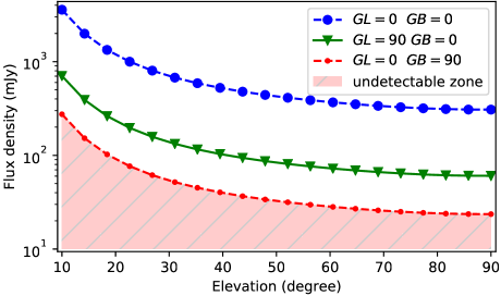
Figure 1: Minimum observable flux density depending on elevation and location of the radio source in the Galaxy for a S/N ratio of 5 and an observation duration of 4h. Three different Galactic temperature and location are used. Blue: Galactic centre ($gl=$$0\text{\,}\mathrm{\SIUnitSymbolDegree}$, $gb=$$0\text{\,}\mathrm{\SIUnitSymbolDegree}$, $T_{\text{sky}}=50000$ K); green: Galactic plane ($gl=$$90\text{\,}\mathrm{\SIUnitSymbolDegree}$, $gb=$$0\text{\,}\mathrm{\SIUnitSymbolDegree}$, $T_{\text{sky}}=8500$ K); red: and outside the Galactic plane ($gl=$$0\text{\,}\mathrm{\SIUnitSymbolDegree}$, $gb=$$90\text{\,}\mathrm{\SIUnitSymbolDegree}$, $T_{\text{sky}}=2350$ K). Pulsars with flux densities in the colored region are too faint, and thus undetectable for the LBA antennas of the LOFAR station FR606.

4 Results

4.1 Detection rates

Out of the 102 pulsating radio sources we observed, we successfully detected 64 pulsars (61 slow pulsars and 3 millisecond pulsars). 12 of these pulsars were either detected in this frequency range for the first time or were detected contemporaneously in this study and in the LOFAR core LBA census (see companion article by Bilous et al., 2019). Most of these ‘new’ low-frequency detections overlap with the simultaneous analysis of LOFAR core data (10 out of 12, cf. Bilous et al., 2019). Compared to Bilous et al. (2019), we detected two additional pulsars (B0105$+$65 and B2021$+$51) that were not in their sample and which were previously undetected at frequencies below 100 MHz.

Figure 2 compares the detected pulsars (blue and magenta points) and the non-detections (red crosses) in terms of measured DM and expected scattering delay at 60 MHz (calculated using the model of Yao et al., 2017) relative to the pulsar period. The two small plots indicate the fraction of detected pulsars as a function of DM (lower panel) and scattering delay (right panel). As expected, pulsars become undetectable once the scatter broadening exceeds the pulsar period (central plot, and right panel). The exception to this rule (B0355$+$54) is discussed in Section 5.2.

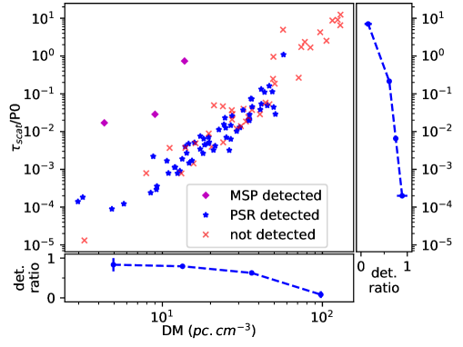
Figure 2: Scattering time in units of the pulsar period versus the dispersion measure for the pulsars of our sample (centre plot, double-logarithmic axes). Detected slow pulsars are shown as blue stars, millisecond pulsars as magenta diamonds, and non-detections as red crosses. Right and bottom panels (with semi-logarithmic axes) shows the fraction of detected pulsars for each axis of the central plot.

Figure 2 also shows a correlation between high DM and high scattering timescales. This correlation is well-known, and has been described, for example, by Bhat et al. (2004). This correlation allows us to estimate the maximum DM at which we can detect pulsars before their pulsations become undetectable due to scatter-broadening. In our case, the maximum detected DM value is $\sim 57$ (for B0355$+$54).

Of course, the DM is related to distance. We can, thus, estimate the maximum distance at which we can detect pulsars. For this, we look at the spatial distribution of our observations and detections. Figure 3 shows the location of our sources in the Galactic plane, with the Earth at the origin of the axes. The electron density model YMW16 from Yao et al. (2017) is represented in a gray scale. Pulsars detected in the present survey are shown as blue dots for normal pulsars and magenta diamonds for the MilliSecond Pulsars (MSPs), and non-detections are shown with red crosses. For this, pulsar distances are derived from the DM using the electron density model YMW16 (Yao et al., 2017). Only pulsars in the Galactic plane are shown (Galactic latitude between $-20\mathrm{°}$ and $20\mathrm{°}$).

A red isocontour denotes a dispersion measure of 100 pc cm^-3 in the Galactic plane ($gb$=$0\mathrm{°}$), corresponding to a scattering time of one second at 60 MHz (derived from the Galactic density model of Yao et al., 2017). With such a scattering delay, even the pulsations from slow pulsars are smeared out and become undetectable. Indeed, we do not have any detection beyond this isocontour. One can see that the red line is at a distance of only a few kpc of the Solar System. Indeed, low-frequency observations of pulsed signals are limited to the nearby population. For comparison, it is possible to observe sources close to the Galactic centre for observations at 1 GHz.

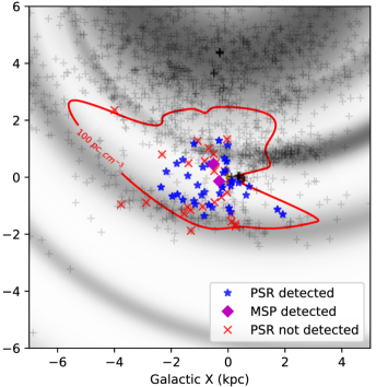
Figure 3: Representation of the census in the Galactic plane with the Earth at the origin of the axes. The electron density model YMW16 (Yao et al., 2017) is represented in grey-scale. Blue stars: detected pulsars. Magenta diamonds: detected MSPs. Red crosses: non-detected pulsars. Only pulsars in the galactic plane are plotted (distance to the galactic plane less than 700 pc). The red line is an isocontour for a DM of $100\text{\,}\mathrm{p}\mathrm{c}\,\mathrm{c}\mathrm{m}^{-3}$. Pulsar distances are derived from the dispersion measure using YMW16 (Yao et al., 2017).

4.2 Detected pulsars

For each detected pulsar, we measured the spin period $P0$, the DM, and the mean flux density, and we calculated the expected scattering delay $\tau_{\text{scat}}^{\text{calc}}$ (derived from the Galactic density model of Yao et al., 2017). These values are detailed in Table 4.2.

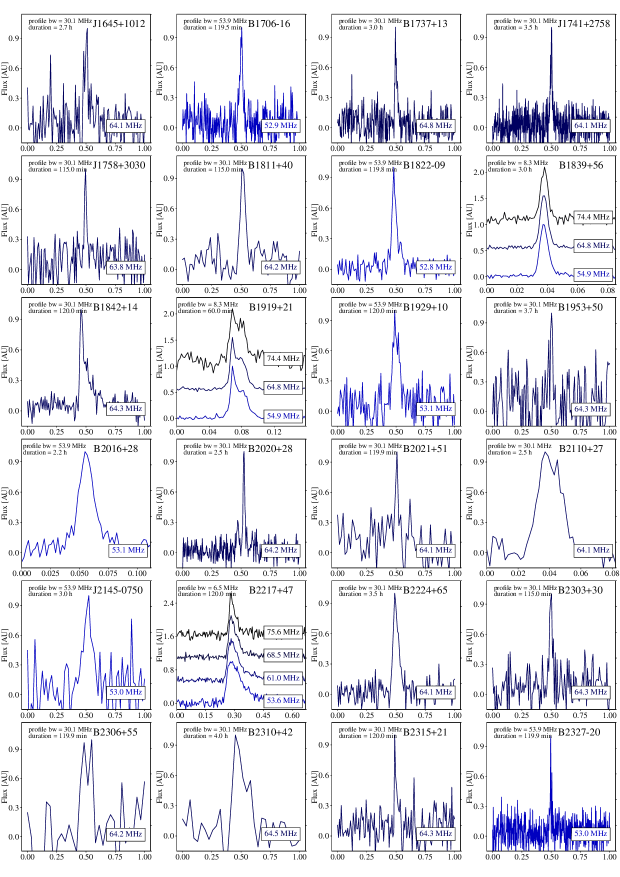
Figure 7: Profiles of the 64 pulsars detected in this study. The profiles are centred on the pulse region. Pulsars with a high S/N are divided into several frequency bands to show frequency-dependent variations in the profiles. At the top left of each sub-figure, the bandwidth and the integration time used for each profile are indicated.

For each detected pulsar, an average pulse profile was generated. These profiles are shown in Figure 7. When the signal-to-noise ratio is sufficient, pulse profiles can be compared at different observing frequencies. This allows us to reveal the frequency dependence of the beam pattern. This is illustrated in Figure 4 for the six pulsars with the best signal-to-noise ratio in our sample:
B0329$+$54 is a mode-switching pulsar (see, e.g. Chen et al., 2011). In the long observation period (1h) shown in Figure 4, we observed a mix of both modes.
Pulsar B0809$+$74 shows drifting sub-pulses and has a frequency-dependent profile. It is discussed in detail in Hassall et al. (2013).
Pulsar B1133$+$16 shows two components where the separation, the amplitudes, and widths are frequency-dependent. This frequency dependence of the beam pattern is visible on Figure 4 and in Hassall et al. (2012).
B1508$+$55 shows pulse echoes which drift across the profile on the timescale of a few years (see Wucknitz, 2019). This is the reason why the profile in Figure 4 is different than that in Bilous et al. (2019).
In contrast to the majority of pulsars detectable at low frequency, the separation between the components of B1919$+$21 decreases with decreasing frequency (see Hassall et al., 2012). In addition, the relative amplitudes of the components seem to be frequency-dependent.
Pulsar B2217$+$47 is highly affected by time-variable scattering (Michilli et al., 2018a; Donner et al., 2019). This effect, convolved with the profile, produces a frequency dependent exponential tail which is clearly visible in Figure 4.

A mean flux density value over the entire band was obtained for each detection (Table 4.2). The measured flux density is assumed to be correct within a 50% accuracy, as was recommended for LOFAR HBA observations (Bilous et al., 2016; Kondratiev et al., 2016) based on the comparison of flux measurements with literature data. This uncertainty includes refractive scintillation, intrinsic flux variation, and imperfections in the beam model used for calibration (Kondratiev et al., 2016). According to our estimates, refractive scintillation represents the dominant effect (at 60 MHz, the timescale for refractive scintillation is of the order of at least one month).

We should note that this estimation was originally established for LOFAR observations in the HBA band (100-200 MHz); for observations with a single station at frequencies below 100 MHz, the situation might be slightly different. This will be studied in more detail in a future paper.

top Pulsars detected in this census. JName, BName: pulsar name. P0: pulsar period. DM: the best-fit DM calculated using pdmp. $\tau^{\text{calc}}_{\text{scat}}$/P0: the scattering time as estimated using YMW16, at 60 MHz divided by the pulsar period, expressed in %. duty cycle: the effective width in pulses profiles (based on w50), expressed in %. S/N: the signal-to-noise-ratio of the detected pulsar profile. duration: total observation length in minutes. $f_{\text{centre}}$: the centre frequency of the observation in MHz. avg.elev: the average elevation during the observation. mean flux: the mean flux density determined for the corresponding centre frequency, with an error bar of 50%. ^σ: pulsed flux density only (due to scatter broadening, part of the pulsar’s energy reaches the telescope as continuum, see Section 5.2). ^τ: the dispersion measure is not corrected for the effect of scatter-broadening (see Section 5.1). ^ϵ: the dispersion measure is not corrected for the effect of intrinsic profile evolution with frequency (see Section 5.1). ^ϵ: the file is folded using an ephemeris file from either Jodrell Bank Observatory or Nançay Radio Observatory (see Section 3.3). J2000 Discovery P0 DM $\tau^{\text{calc}}_{\text{scat}}$/P0 duty SNR duration $f_{\text{centre}}$ avg.elev mean
NameName [s] [pc cm^-3] [%] cycle [%] [min] [MHz] degrees flux [mJy]
Continued from previous page
J2000 Discovery P0 DM $\tau^{\text{calc}}_{\text{scat}}$/P0 duty SNR duration $f_{\text{centre}}$ avg.elev mean
NameName [s] [pc cm^-3] [%] cycle [%] [min] [MHz] degrees flux [mJy]
Continued on next page

llllllllllll J0014$+$4746 & B0011$+$47 1.241^ϵ 30.30(2) 1.3 4.4 9 240 65 79 43(21)
J0030$+$0451 J0030$+$0451 0.005 4.33320(6) 1.7 4.9 9 180 53 46 86(43)
J0034$-$0534 J0034$-$0534 0.002 13.76580(4)^τ 73.8 46.6 55 180 53 32 855(428)
J0034$-$0721 B0031$-$07 0.943 10.916(5) 0.1 15.3 41 120 53 35 560(280)
J0051$+$0423 J0051$+$0423 0.355 13.9265(5) 0.4 5.3 14 120 53 46 30(15)
J0056$+$4756 B0053$+$47 0.472 18.14(1) 0.6 6.5 17 135 65 84 102(51)
J0108$+$6608 B0105$+$65 1.284 30.56(2) 1.3 4.0 11 325 65 67 74(37)
J0141$+$6009 B0138$+$59 1.223 34.931(2) 2.2 10.8 28 120 65 68 242(121)
J0152$-$1637 B0149$-$16 0.833 11.9289(5) 0.1 10.4 37 120 53 25 215(107)
J0323$+$3944 B0320$+$39 3.032 26.20(1) 0.3 20.8 31 165 65 73 127(63)
J0332$+$5434 B0329$+$54 0.715 26.768(1) 1.5 11.2 119 60 65 51 1841(921)
J0358$+$5413 B0355$+$54 0.156 57.15(1)^τ 109 7.9 9 240 65 77 129(64)^σ
J0454$+$5543 B0450$+$55 0.341 14.5921(10) 0.5 8.7 28 325 53 53 124(62)
J0528$+$2200 B0525$+$21 3.746 50.90(2)^ϵ 2.9 13.7 31 120 53 61 257(128)
J0611$+$30 J0611$+$30 1.412 45.31(4) 4.9 4.5 9 240 65 68 64(32)
J0630$-$2834 B0628$-$28 1.244 34.42(1) 2.0 7.9 23 55 65 14 1076(538)
J0700$+$6418 B0655$+$64 0.196^ϵ 8.7749(2) 0.2 10.7 33 120 53 68 95(47)
J0814$+$7429 B0809$+$74 1.292 5.7578(9)^ϵ 0.0 45.9 252 60 53 62 1630(815)
J0820$-$1350 B0818$-$13 1.238 40.962(10) 3.8 2.7 10 115 65 28 61(31)
J0826$+$2637 B0823$+$26 0.531 19.4743(8) 0.7 14.2 79 60 65 63 423(212)
J0837$+$0610 B0834$+$06 1.274 12.864(2)^ϵ 0.1 6.9 309 60 65 44 1268(634)
J0908$-$1739 B0906$-$17 0.402 15.875(2) 0.5 1.5 5 180 53 24 29(15)
J0922$+$0638 B0919$+$06 0.431 27.2965(5) 2.6 15.4 144 180 65 42 550(275)
J0927$+$23 J0927$+$23 0.762 23.127(2) 0.8 0.5 6 215 62 54 12(6)
J0946$+$0951 B0943$+$10 1.098 15.3291(5) 0.2 15.2 148 150 53 46 610(305)
J0953$+$0755 B0950$+$08 0.253 2.9711(2)^ϵ 0.0 14.6 140 60 62 41 2276(1138)
J1115$+$5030 B1112$+$50 1.656 9.197(3) 0.0 2.5 12 275 53 75 21(11)
J1136$+$1551 B1133$+$16 1.188 4.8468(7)^ϵ 0.0 18.7 261 120 53 53 894(447)
J1238$+$2152 J1238$+$2152 1.119 17.967(3) 0.3 4.1 15 155 65 62 38(19)
J1239$+$2453 B1237$+$25 1.382 9.2562(8)^ϵ 0.0 0.2 50 170 62 65 102(51)
J1313$+$0931 J1313$+$0931 0.849 12.0318(5) 0.1 2.2 7 215 57 48 25(13)
J1321$+$8323 B1322$+$83 0.670^ϵ 13.28(3) 0.2 1.4 5 225 53 43 16(8)
J1509$+$5531 B1508$+$55 0.740 19.616(1) 0.5 10.7 378 360 65 73 943(471)
J1532$+$2745 B1530$+$27 1.125 14.697(6) 0.1 6.0 18 240 53 66 69(35)
J1543$-$0620 B1540$-$06 0.709 18.372(4) 0.4 9.0 22 145 65 34 143(72)
J1543$+$0929 B1541$+$09 0.748 34.950(5) 3.5 5.6 26 90 53 50 541(270)
J1607$-$0032 B1604$-$00 0.422 10.6823(5) 0.2 9.9 64 60 53 42 575(288)
J1614$+$0737 B1612$+$07 1.207 21.401(2) 0.4 3.8 24 165 65 48 120(60)
J1635$+$2418 B1633$+$24 0.491^ϵ 24.24(1) 1.5 3.9 8 210 65 56 68(34)
J1645$-$0317 B1642$-$03 0.388 35.7589(5) 7.4 8.8 48 240 65 37 420(210)
J1645$+$1012 J1645$+$1012 0.411 36.165(6) 7.3 4.6 12 165 65 50 108(54)
J1709$-$1640 B1706$-$16 0.653 24.892(2) 1.3 7.3 17 120 53 25 317(159)
J1740$+$1311 B1737$+$13 0.803 48.660(5)^τ 11.3 4.6 14 180 65 36 131(66)
J1741$+$2758 J1741$+$2758 1.361 29.168(8) 1.0 9.6 21 210 65 67 54(27)
J1758$+$3030 J1758$+$3030 0.947 35.08(1) 2.8 2.0 8 115 65 67 26(13)
J1813$+$4013 B1811$+$40 0.931 41.60(2) 5.4 2.1 11 115 65 57 68(34)
J1825$-$0935 B1822$-$09 0.769 19.386(2) 0.5 5.7 33 120 53 32 2502(1251)
J1840$+$5640 B1839$+$56 1.653 26.773(2) 0.6 7.0 166 180 65 57 481(240)
J1844$+$1454 B1842$+$14 0.375 41.483(2)^τ 13.2 6.7 36 120 65 51 773(386)
J1921$+$2153 B1919$+$21 1.337 12.437(2) 0.1 8.4 180 60 65 63 1586(793)
J1932$+$1059 B1929$+$10 0.227 3.186(2) 0.0 5.8 15 120 53 41 306(153)
J1955$+$5059 B1953$+$50 0.519 31.990(5) 3.7 1.2 5 225 65 70 16(8)
J2018$+$2839 B2016$+$28 0.558 14.1982(5) 0.3 8.6 37 135 53 54 243(121)
J2022$+$2854 B2020$+$28 0.343 24.6315(10) 2.3 6.2 30 150 65 69 243(122)
J2022$+$5154 B2021$+$51 0.529 22.541(6) 1.1 1.3 6 120 65 81 46(23)
J2113$+$2754 B2110$+$27 1.203 25.121(3) 0.7 8.4 37 150 65 65 143(71)
J2145$-$0750 J2145$-$0750 0.016^ϵ 9.0058(2) 2.9 3.5 8 180 53 34 59(30)
J2219$+$4754 B2217$+$47 0.538 43.492(1)^τ 11.0 15.6 125 120 65 76 1239(620)
J2225$+$6535 B2224$+$65 0.683 36.473(4) 4.5 5.5 29 210 65 46 293(146)
J2305$+$3100 B2303$+$30 1.576 49.60(3) 6.2 4.1 11 115 65 72 45(22)
J2308$+$5547 B2306$+$55 0.475^ϵ 46.57(4)^τ 16.2 2.3 5 120 65 70 170(85)
J2313$+$4253 B2310$+$42 0.349 17.282(8) 0.8 2.6 11 240 65 60 81(41)
J2317$+$2149 B2315$+$21 1.445 20.876(5) 0.3 3.7 10 120 65 59 35(18)
J2330$-$2005 B2327$-$20 1.644 8.4554(10) 0.0 4.0 16 120 53 22 111(55)

Figure 4: Frequency-dependent profiles for the six pulsars with the best S/N in our sample. Profiles are zoomed in on the on-pulse region.

4.3 Upper limits for non-detections

For each non-detection, we computed an upper limit for the mean flux density according to Equation (1) in Section 3.6. The resulting values are given in Table A. Depending on source position and observation time, we obtained upper limits between $\sim 60$ and 4500 mJy, which is compatible with our initial expectation (Figure 1).

Compared to previous observations, only 20 pulsars previously detected below 100 MHz have either not been observed or not been detected. Of these, one (J0437$-$4715) is not observable for FR606 and seven others have not been observed as part of this survey. This leaves 13 previously reported pulsars which we have not detected, some of which were reported as faint or marginal detections:
B0226$+$70 was detected by the LOFAR core LBA census (Bilous et al., 2019) with a mean flux density of 49 mJy, which is consistent with our upper limit of 329 mJy.
B0301$+$19 has been reported by Izvekova et al. (1981, $\sim$40 mJy at 61 MHz), by Stovall et al. (2015, 120$\pm$60 mJy at 64.5 MHz), and has been detected in the LOFAR core LBA census (Bilous et al., 2019, 61$\pm$33 mJy at 50 MHz). Our upper limit is 121 mJy, which is compatible with all of these detections.
B0609$+$37 was detected by the LOFAR core LBA census (Bilous et al., 2019) with a mean flux density of 46 mJy, which is consistent with our upper limit of 664 mJy.
B0611$+$22 and B0656$+$14 were previously reported as a detections with flux densities (Izvekova et al., 1981, 180 mJy and 60 mJy at 85 MHz respectively), which are compatible with our upper limits of 337 mJy and 77 mJy.
We expected to detect J0921$+$6254 (detected in Pilia et al., 2016, but with no measured flux density). The pulsar was detected by the LOFAR core LBA census (Bilous et al., 2019) with a mean flux density of 41$\pm$22 mJy, which is consistent with our upper limit of 58 mJy.
B0940$+$16 was a weak detection in Zakharenko et al. (2013, 7.3 mJy at 25 MHz), which is compatible with our upper flux limit of 430 mJy (taking into account their spectral index of $\alpha=2.31$).
B1749$-$28 has been reported twice (Izvekova et al., 1981; Stovall et al., 2015), but is at very low elevation for FR606, which strongly reduced the efficiency of the antenna array. This is reflected in our poorly constraining upper limit of 4533 mJy, which is compatible with the previous detections.
B1839$+$09 was detected by the LOFAR core LBA census (Bilous et al., 2019) with a mean flux density of 190 mJy, which is consistent with our upper limit of 521 mJy.
J1851$-$0053 and J1908$+$0734 were weak detections in Zakharenko et al. (2013, 7 mJy for both pulsars at 25 MHz). Our upper flux limit of 578 mJy and 203 mJy are compatible with their data and constrains the spectral index to values $<5$ and $<4$ respectively.
Based on Zakharenko et al. (2013, 27 mJy at 25 MHz), we hoped to detect B1944$+$17. Still, their values are compatible with our upper limit of 110 mJy (taking into account their spectral index of $\alpha=1.22$).
Based on Zakharenko et al. (2013, 15 mJy at 25 MHz), we hoped to detect B1952$+$29 for which we have an upper limit of 124 mJy. Our non-detection is compatible with their data and constrains the spectral index to values $<2.5$.
Besides the lack of sensitivity, other possible reasons for non-detections are discussed in Section 5.6.

5 Discussion

5.1 Dispersion at low frequency

In Section 4.2, we present DM values for all pulsars detected in this census. To obtain these values, we used pdmp, which modifies the DM value until the S/N of the pulse profile is maximised.

This approach does not correctly take into account frequency-dependent pulse profile variations. A typical example for this would be a pulsar with two or more bright components, whose flux ratio changes as a function of frequency such as B1133$+$16 and B0809$+$74 (cf. Figure 4).

A similar situation arises for pulsars that are scatter-broadened. In that case, part of the scatter-broadening ($\propto$ $f^{-4}$) is absorbed by pdmp, resulting in an erroneous extra correction of the DM ($\propto$ $f^{-2}$), especially at low frequencies.

An ideal de-dispersion process should use a 2D template, either based on Gaussian fits (Pennucci et al., 2014; Liu et al., 2014) or based on the smoothed dataset (e.g. Donner et al., 2019). In addition, a fiducial point would be required (e.g. Hassall et al., 2012) in order to disentangle dispersion and frequency-dependent profile variation. Without this, the absolute DM cannot be measured.

We did not apply any of these methods in this publication, which limits the DM precision for some of the pulsars in this census. These pulsars are clearly labelled in Table 4.2.

5.2 Dispersion, scattering, and detection rate

As discussed in Section 4.1, dispersion and scattering are correlated. Indeed, Figure 2 shows that the measured DM and the calculated scattering time from YMW16 are correlated in our sample of detected pulsars. The detection rates decrease for high scattering time and high DM. Low-frequency observations are highly affected by the dispersion introduced by the interstellar medium. However, this effect is corrected using coherent de-dispersion (Hankins & Rickett, 1975; Bondonneau et al., 2019).

Consequently, the low detection rate in high DM is not due to the dispersion, but caused by the multi-path propagation in the interstellar medium which is usually described by a convolution between the pulse profile and an exponential function. The result is an exponential tail characterised by the scattering time $\tau$, as can be seen, for example, with B2217$+$47 in Figure 7. For some pulsars, the scattering time is greater than the rotational period and the pulsations disappear during the folding process. This is the reason why some of the radio sources (J0324$+$5239, B0531$+$21, B0540$+$23, B0611$+$22, B0626$+$24, B1931$+$24, B1946$+$35, B2148$+$63, and B2227$+$61) are not detected: their scattering time exceeds the pulsar’s period (cf. Figure 2 and Table A).

For B0355$+$54, the estimated scattering time slightly exceeds the pulse period (Table 4.2). With this, the pulsar should still remain visible, which is indeed the case (see Figure 7). Since part of the pulsar’s energy reaches the telescope as continuum rather than pulsed emission, the measured flux density only represents the pulsed flux.

We compared the scattering times obtained with YMW16 (Yao et al., 2017) to those given by a different Galactic density model, namely, NE2001 (Cordes & Lazio, 2002). The latter model seems to underestimate the scattering with respect to YMW16 and to the value deduced from our own observed profiles (Figure 7). This is true in particular for B0355$+$54, B2217$+$47 and B2306$+$55, where the values given by NE2001 are, respectively, 11.6%, 1.4%, and 3.4% of the phase, numbers that are far from those extracted based on our own observed profiles or from the values provided by the electron density model YMW16, namely 108.7%, 11.0%, and 16.2% (cf. Table 4.2, column 5).

We note that for some pulsars, the measured scattering index $\alpha_{\text{scat}}$ (defining the frequency dependence of the scattering time $\tau_{\text{scat}}$) obtained from observations can deviate considerably from the theoretical value of 4.0 or 4.4 used in models such as in Yao et al. (2017). In particular, Geyer et al. (2017) analysed LOFAR observations at 150 MHz and found a less steep behaviour for B0114$+$58, B0540$+$23 and B0611$+$22. If this is confirmed and can be extended to our observing frequency of 60 MHz, the resulting scattering time would be lower and the pulsars would not be rendered undetectable by scattering. In that case, the non-detection of these specific pulsars would be caused by a different reason (see e.g. Section 5.6).

5.3 Spectral turnover: comparison with HBA census (110-188 MHz)

The 39 pulsars of the FR606 LBA census (25-80 MHz) described in this publication have also been detected in the LOFAR HBA census (Bilous et al., 2016, 110-188 MHz). The spectral index and turnover frequency given in Bilous et al. (2016) can be used to estimate a theoretically expected mean flux density for the LBA frequency range and to compare it to our measurements.

Figure 5 compares the mean flux densities obtained from the present LBA census (X-axis) to the theoretical mean flux density extrapolated from Bilous et al. (2016) (Y-axis). Pulsars are represented with a blue dot if Bilous et al. (2016) identified a turnover, and a red triangle otherwise (i.e. the spectrum was fitted using only one spectral index). For FR606 observations, we indicate the nominal error resulting from the flux calibration. The systematic error of 50% is represented by the green surface around the diagonal line of equal fluxes.

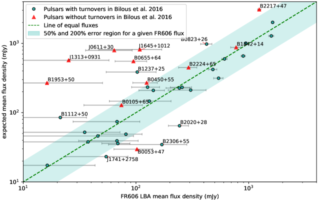
Figure 5: Comparison of the mean flux densities reported in this paper with those obtained from the fitted spectral indices in Bilous et al. (2016). Blue dots: pulsars fitted with at least one turnover in their spectrum. Red triangles: pulsars fitted with a single spectral index. The line of equal flux values is shown by a green dashed line. In order to maintain symmetry between the two axes, we take a range from 50-200 % of the equal flux value (green area) for the systematic error.

For most pulsars, the measured and the extrapolated mean flux densities agree within the error range. The exceptions are the following:
For five of the pulsars (J0611$+$30, B0655$+$64, J1313$+$0931, J1645$+$1012, and B1953$+$50), the mean flux density extrapolated from the HBA range is considerably higher than the flux density we measured in the LBA range. For these pulsars, Bilous et al. (2016) give a simple power-law without turnover. Our observations show a considerable lack of flux density below 100 MHz, indirectly showing that these pulsars do indeed have a spectral turnover at low frequencies. Similarly, in the companion article, Bilous et al. (2019) find that a low-frequency turnover is compatible with the flux density measurements of J0611$+$30, J1313$+$0931 and J1645$+$1012. Similarly, but with a lower significance, we see a hint for a turnover for B2217$+$47.
For B1112$+$50, the extrapolated flux is overestimated with respect to the measurement. It is, however, consistent with the HBA flux measured in in Bilous et al. (2016, see their Figure C.6). The extrapolation takes this HBA flux into account, but also (older) literature values, suggesting possible time variability of this pulsar.
For B1237$+$25, the expected mean flux density is overestimated even though Bilous et al. (2016) fit a spectral turnover. The model uses three frequency ranges with different spectral indices. We suspect that the turnover happens at slightly higher frequency than the 45 MHz estimated in Bilous et al. (2016, see their Figure C.6).
For B2020$+$28 the spectral index of the extrapolation is not well constrained. A shallower spectral index at low frequencies is compatible with both previous observations and our LBA data.

This comparison of observations at frequencies below 100 MHz (our work) to observations above 100 MHz (Bilous et al., 2016) shows that several pulsars which used to be described using a single power-law have a spectral turnover. This does not come as unexpected: Bilous et al. (2016) found that the average spectral index is lower for measurements at 150 MHz than for higher frequencies (potentially indicating proximity to a turnover) and noted that measurements below 100 MHz are required to study the phenomenon of turnover systematically.

For a number of pulsars which were modelled without spectral turnover (Bilous et al., 2016), our measured flux density is in agreement with the extrapolated flux density value. This indicates that these pulsars either have no turnover or (more likely) that the turnover occurs at frequencies below our sensitivity maximum ($\sim 58$ MHz). Again, more high sensitivity observations below 100 MHz are required for a systematic study.

The comparison presented above is just a first step. A detailed analysis of spectral indices and turnover frequencies will be presented in a companion publication for the brightest pulsars in our sample (Bondonneau et al. in prep), and more sensitive observations will be provided by NenuFAR in the near future.

5.4 Comparison with the LOFAR LBA census

In a companion study, we observed pulsars with the LBA antennas of the LOFAR core (Bilous et al., 2019). Between both studies, there are in total 64 common radio sources. Of these, 36 pulsars were detected by both FR606 and the LOFAR core, 5 were detected only by the LOFAR core, 1 was detected only by FR606, and 22 were not detected by either instrument.

5.4.1 Common detections

Figure 6 shows the measured flux densities from the LOFAR Core LBA census (Y-axis) reported by Bilous et al. (2019) in comparison with the flux density measurements from the current FR606 census (X-axis). For FR606 and LOFAR Core observations, we indicate the nominal error resulting from the flux calibration. The systematic error of 50% is represented by the green surface around the diagonal dashed line of equal fluxes.

For all of the 36 pulsars that were detected in both censuses, the measured flux densities are compatible or almost compatible within the uncertainties.

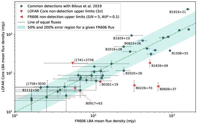
Figure 6: Comparison of mean flux densities reported in this paper with those obtained by Bilous et al. (2019). The line of equal flux values is shown by green dashed line. In order to maintain symmetry between the two axes, for the systematic error we take a range from 50-200 % of the equal flux value (green area) Red triangles show the flux density upper limits when a pulsar was detected only by FR606 LBA (triangle is pointing down), or only by LOFAR Core (triangles are pointing left). Note that for the upper limits for the LOFAR Core we used the value of $3\sigma$, where $\sigma$ is the nominal uncertainty on the flux following Bilous et al. (2016), while for the FR606 upper limits, we used Equation (1) from the present paper.

Some of the values are not perfectly matched (e.g. B1508$+$55, B1919$+$21, B1929$+$10). This can be attributed to a number of reasons (see, e.g., Kondratiev et al., 2016), such as the contribution of strong background sources to the wide low-frequency beam, beam jitter caused by the ionosphere, refractive scintillation (RISS), or intrinsic variability. Each of these factors can increase or decrease the measured flux density. For instance, both the censuses were performed at different epochs so that RISS could affect the measurements differently. For the pulsars B1508$+$55 and B2020$+$28, FR606 has measured a slightly higher flux density than the LOFAR core. This could be explained by ionosphere jitter during the LOFAR Core census observations (the field of view of the international station is wider, so that a small shift of the beam should not matter for our FR606 observations). Indeed, Bilous et al. (2019) used multiple beams simultaneously and found a higher flux density in one of the off-centre beams for several pulsars (including B1508$+$55).

The same factors could potentially lead to non-detections by one of the telescopes or by both. Figure 6 includes pulsars detected by at least one of the telescopes. In case of non-detection by one of the telescopes, we use the upper limit value on flux density.

5.4.2 Pulsars detected only by LOFAR core

Five of the pulsars seen with the LOFAR Core have not been detected by FR606, namely PSRs B0226$+$70, B0301$+$19, B0609$+$37, B0917$+$63, and B1839$+$09. For all of these non-detections, the upper limits deduced from our FR606 observations are compatible with the measured flux densites of the LOFAR core (see Figure 6). The non-detection of B0917$+$63 by FR606 in 275 minutes came as a bit of a surprise. It is possible that the RISS leads to intensity variations. Still, the upper limit of FR606 is compatible with the measured flux density from the LOFAR core.

5.4.3 Pulsars detected only by FR606

PSR J1741$+$2758 was not detected with the LOFAR Core in 23 minutes, whereas it was detected by FR606 in 210 minutes. The smaller effective area of FR606 (96 dipoles of FR606 vs. 24x48 dipoles of the Core) is balanced out by the longer integration time. Also, for the LOFAR Core observation, this particular dataset was of poor quality (more than half of the band was deleted due to dropped packets; see Bilous et al., 2019).

The non-detection by the LOFAR Core yields an upper flux density limit which is compatible with the detection by FR606. We also note that this pulsar had already been detected at frequencies below 100 MHz before (Zakharenko et al., 2013).

5.5 Millisecond pulsars

Currently, radio detections at frequencies below 100 MHz have been published for four millisecond pulsars (Dowell et al., 2013; Kondratiev et al., 2016; Bhat et al., 2018), of which three are observable by FR606. We have observed and detected all three of these pulsars. In view of the low flux densities of these pulsars, we did not include any other millisecond pulsars in our sample.

5.6 Possible reasons for non-detections

There are a number of potential reasons for non-detections:
The spectrum (as characterised by the spectral index $+$ turnover) is not favourable for very low frequency observations.
In principle, the pulse period or DM could be outside the range of values probed by pdmp. However, all of our pulsars have been previously detected below 200 MHz, so we expect the range in DM to be large enough. As we have used updated ephemeris files, we also expect the range in pulse period to be sufficient.
The pulse is smeared by scatter-broadening. This is the case, for example, for the Crab pulsar B0531$+$21, where the scattering time is about 500% of the pulse period. For a number of the pulsars in Table A, the expected scatter broadening is high ($\tau_{\text{scat}}^{\text{calc}}/P0>1$), which is indeed compatible with our non-detection. See Section 5.2 for details.
Intermittent emission such as nulling or mode-changing can affect a pulsars detectability. For example, B0943$+$10 (Hermsen et al., 2013; Bilous et al., 2014) and B0823$+$26 (Sobey et al., 2015) are known for their mode-changing behaviour at low frequencies. For mode-changing pulsars, the mean flux density depends on the state of the pulsar during the observation, which can make the difference between a detection and a non-detection. The same is, of course, true for nulling pulsars.
Diffractive scintillation should not affect our measurements because the decorrelation bandwidths should be lower than our bandwidth and, thus, many scintles are averaged out.
Slow fluctuations of the pulsar amplitudes can be caused by refractive scintillation by the interstellar medium. For observations at 74 MHz, Gupta et al. (1993) measured modulation indices (ratio of the standard deviation of the observed flux densities to their mean) in the range of 0.15-0.45, which can account for some of our non-detections. The bandwidth they used was of 500 kHz, which is much lower than our bandwidth. However, refractive scintillation is broadband in nature (Narayan, 1992) so bandwidth should not matter.
Some of the flux density values given in earlier publications can be over-estimations, especially for the cases with a low S/N.

6 Conclusion

In this publication, we observed a total of 102 pulsars, of which 64 were detected successfully. Two of these had never before been detected at frequencies below 100 MHz.

We obtained results similar to those in the companion study using the LOFAR core (Bilous et al., 2019). We were able to partially compensate for the lower effective area ($\sim$10%) with longer integrations during RFI-quiet moments (thus optimising the quality of the data). Due to the lower sensitivity of FR606, we did not detect all the pulsars detected by Bilous et al. (2019) but our upper limits are compatible with their flux density measurements. We detected two pulsars that were not part of the sample of Bilous et al. (2019), and one pulsar (J1741$+$2758) that was a non-detection in that study.

For several pulsars (J0611$+$30, B0655$+$64, J1313$+$0931, J1645$+$1012, and B1953$+$50), the comparison to observations at slightly higher frequencies (Bilous et al., 2016) indicates a previously unknown spectral turnover. This confirms the expectation that spectral turnovers are a widespread phenomenon and that measurements below 100 MHz are essential to studying this phenomenon systematically.

We should note that the pulsar population represented in this census is biased by the selection method, essentially based on the previous detections of (Stovall et al., 2015; Pilia et al., 2016; Kondratiev et al., 2016; Bilous et al., 2016). It does not take into account pulsars that have not been detected in the HBA range.

In order to further study the population statistics of these low-frequency pulsars, a more homogeneous and substantial dataset is required. This will be reached by the NenuFAR radio telescope (Zarka et al., 2012, 2014, 2015) and its pulsar instrumentation LUPPI (Bondonneau et al., 2019), which we are currently using to conduct a systematic census of the known pulsar population (Bondonneau et al. in prep). NenuFAR, while providing us with an equivalent sensitivity to the LOFAR core at 60 MHz, offers a flat gain response across the LBA frequency band (from 10-85 MHz). Consequently, a much higher detection rate can be expected than for the present census. In addition, the flat frequency response will allow a much higher sensitivity towards frequency-dependent effects such as dispersion, scattering, spectral turnovers, and pulsar profile evolution.

Appendix A Non-detection Table

top Pulsars that were not detected in this census. JName, BName: pulsar name. P0: pulsar period. DM: the DM used to coherently disperse the observations from Zakharenko et al. (2013) Stovall et al. (2015) and Bilous et al. (2016), and ATNF to complete. $\tau^{\text{calc}}_{\text{scat}}$/P0 : the scattering time (estimated using YMW16 Yao et al. (2017) at 60 MHz) divided by the pulsar period. duration: total duration of the observation in minutes. elev: the average elevation of the observation. upper limit for the mean flux: The upper limit for the mean flux density 1. ^η: excluding the contribution of the nebula to $T_{\text{sky}}$. ^τ: upper limit for the mean flux density is not valid ($\tau^{\text{calc}}_{\text{scat}}/$P0¿ 100 %). ^ϵ: the file is folded using an ephemeris file from either Jodrell Bank Observatory or Nançay Radio Observatory (see Section 3.3). J2000 Discovery P0 DM $\tau^{\text{calc}}_{\text{scat}}$/P0 duration elev upper limit for the
Name Name sec pc.cm^-3 % min degree mean flux density [mJy]
Continued from previous page
J2000 Discovery P0 DM $\tau^{\text{calc}}_{\text{scat}}$/P0 length elev upper limit for the
Name Name sec pc.cm^-3 % min degree mean flux density [mJy]
Continued on next page


lllllllll J0117$+$5914 & B0114$+$58 0.1014 49.4230 95.3 255 64 344^τ
J0139$+$5814 B0136$+$57 0.2725^ϵ 73.7790 172.6 225 63 366^τ
J0231$+$7026 B0226$+$70 1.4668^ϵ 46.6400 5.3 240 45 329
J0304$+$1932 B0301$+$19 1.3876^ϵ 15.7370 0.1 240 53 121
J0324$+$5239 J0324$+$5239 0.3366 119.0000 984.6 240 56 281^τ
J0415$+$6954 B0410$+$69 0.3907^ϵ 27.4650 2.9 360 44 253
J0534$+$2200 B0531$+$21 0.0334 56.7875 497.4 60 43 705^η,τ
J0543$+$2329 B0540$+$23 0.2460^ϵ 77.7115 235.8 120 61^τ 428^τ
J0612$+$3721 B0609$+$37 0.2980^ϵ 27.1350 3.7 110 42 664
J0614$+$2229 B0611$+$22 0.3350^ϵ 96.9100 426.0 240 61 337^τ
J0629$+$2415 B0626$+$24 0.4766^ϵ 84.1950 168.4 180 48 540^τ
J0653$+$8051 B0643$+$80 1.2144^ϵ 33.3320 1.8 240 56 316
J0659$+$1414 B0656$+$14 0.3849^ϵ 13.9770 0.4 240 53 77
J0921$+$6254 B0917$+$63 1.5680^ϵ 13.1580 0.1 275 51 58
J0943$+$1631 B0940$+$16 1.0874^ϵ 20.3200 0.4 115 58 430
J0943$+$22 J0943$+$22 0.5329 25.1000 1.6 360 65 24
J0947$+$27 J0947$+$27 0.8510^ϵ 29.0000 1.6 220 65 1344
J1503$+$2111 J1503$+$2111 3.3140 3.2600 0.0 360 48 57
J1612$+$2008 J1612$+$2008 0.4266 19.5440 0.9 240 56 298
J1627$+$1419 J1627$+$1419 0.4909 33.8000 4.8 180 55 415
J1649$+$2533 J1649$+$2533 1.0153^ϵ 35.5000 2.8 240 64 303
J1720$+$2150 J1720$+$2150 1.6157 41.1000 3.0 240 57 292
J1740$+$1000 J1740$+$1000 0.1541^ϵ 23.8500 4.6 120 43 501
J1752$-$2806 B1749$-$28 0.5626 50.3720 18.5 60 14 4533
J1841$+$0912 B1839$+$09 0.3813^ϵ 49.1070 24.8 120 50 521
J1851$-$0053 J1851$-$0053 1.4091 24.0000 0.5 240 38 578
J1907$+$4002 B1905$+$39 1.2358^ϵ 30.9600 1.4 250 53 262
J1908$+$0734 J1908$+$0734 0.2124 11.1040 0.4 360 45 203
J1933$+$2421 B1931$+$24 0.8137 105.9251 252.3 120 64 468^τ
J1946$+$1805 B1944$+$17 0.4406^ϵ 16.2200 0.5 120 59 110
J1948$+$3540 B1946$+$35 0.7173 129.0750 646.7 120 77 391^τ
J1954$+$2923 B1952$+$29 0.4267^ϵ 7.9320 0.1 115 54 124
J2043$+$2740 J2043$+$2740 0.0961^ϵ 21.0000 4.9 115 56 425
J2055$+$2209 B2053$+$21 0.8152^ϵ 36.3610 3.8 120 64 419
J2139$+$2242 J2139$+$2242 1.0835 44.1000 5.8 115 57 427
J2149$+$6329 B2148$+$63 0.3801^ϵ 128.0000 1178.8 120 72 1798^τ
J2157$+$4017 B2154$+$40 1.5253^ϵ 70.8570 26.2 180 36 399
J2229$+$6205 B2227$+$61 0.4431 124.6140 905.6 180 47 400^τ

Appendix B Pulsar profiles