Spin-Polaronic Effects in Electric Shuttling in a Single Molecule Transistor with Magnetic Leads

Abstract

Current-voltage characteristics of a spintromechanical device, in which spin-polarized electrons tunnel between magnetic leads with anti-parallel magnetization through a single level movable quantum dot, are calculated. New exchange- and electromechanical coupling-induced (spin-polaronic) effects that determine strongly nonlinear current-voltage characteristics were found. In the low-voltage regime of electron transport the voltage-dependent and exchange field-induced displacement of quantum dot towards the source electrode leads to nonmonotonic behavior of differential conductance that demonstrates the lifting of spin-polaronic effects by electric field. At high voltages the onset of electron shuttling results in the drop of current and negative differential conductance, caused by mechanically-induced increase of tunnel resistivities and exchange field-induced suppression of spin-flips in magnetic field. The dependence of these predicted spin effects on the oscillations frequency of the dot and the strength of electron-electron correlations is discussed.

The ability to control the spin of electrons by electrical 1 ; 2 ; 3 , magnetic 4 and optical 5 means has generated various applications in modern physics. Spin-controlled nanoelectromechanics fedorets1 is a promising new direction in nanoelectronics where the interplay of spin- and mechanical degrees of freedom can lead to novel electron transport phenomena involving the spin and charge of electrons that can not be observed in “ordinary” single electron transistors. Electron shuttling (see Ref. shuttle, and experimental papers Refs. exp1, ; exp2, ; exp3, ) induced by the magnetic exchange forces present in a single-electron transistor with magnetic leads was discussed in Ref. msh, . Unlike in a standard single-electron shuttle fedorets , where the electric field generated by a bias voltage always drives the charged quantum dot (QD) from the source- to the drain electrode, the exchange interaction between an electron spin in the dot and the magnetization of the source electrode results in an attractive exchange force (in what follows we assume that the source electrode only contains spin-up electrons and the drain electrode only spin-down electrons). For half-metallic leads with opposite magnetization directions (see Fig. 1) the electrical current through the system is blocked as long as the electron spin-projection is conserved and one needs to induce spin flips to lift this “spin blockade”.

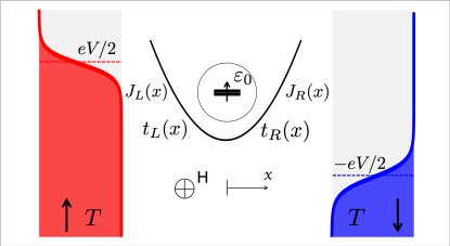
Figure 1: Sketch of the single-molecule transistor with magnetic leads discussed in the text (modelled by a single-level vibrating quantum dot). The dot couples to the fully and oppositely magnetized electrodes (spin-up electrons in the left- and spin-down electrons in the right lead) with position-dependent tunneling $t_{L/R}(x)$ and exchange $J_{L/R}(x)$ couplings. The electrons in the leads are described by equilibrium Fermi distribution functions, characterized by different chemical potentials $\mu_{L}-\mu_{R}=eV$ ($V$ is the bias voltage) but the same temperature $T$. A weak external magnetic field is applied perpendicular to the direction of the current and to the magnetization in the leads: $H\ll\Gamma/g\mu_{B}$ ($g$ is the gyromagnetic ratio, $\mu_{B}$ is the Bohr magneton and $\Gamma$ is level width, when the dot is located at the midpoint between the leads).

In a magnetic shuttle device the spin blockade is lifted by an external magnetic field perpendicular to both the tunneling direction and the magnetization in the leads. This magnetic field induces oscillations between the spin-up and spin-down projections of the spin of an electron in the dot, thus allowing an electrical current to flow through the system. Another effect of these oscillations is that during the time the quantum dot contains an electron in the spin-down state it is attracted to the drain- rather than to the source electrode. This is a necessary condition for shuttling and magnetic shuttling is indeed realized msh in weak magnetic fields, $g\mu_{B}H\lesssim g\mu_{B}H_{c}=\sqrt{3[\Gamma^{2}+(\hbar\omega)^{2}]}$, where $\mu_{B}$ is the Bohr magneton, $g$ is the gyromagnetic ratio, $\Gamma$ is the dot-lead tunneling coupling (the width of the QD energy level), and $\omega$ is the angular frequency of the QD mechanical oscillations.

The theory of magnetic shuttling developed in Refs. msh, , thsh, , and ilinskaya, neglects the electric driving force. This is a good approximation for small bias voltages when the exchange forces on the QD are much stronger than the electric force acting on it, while for larger bias voltages both types of forces must be taken into account. The interplay then occurring between the electric and magnetic driving forces in a single-electron magnetic shuttle is the subject of the present work.

In what follows we consider a symmetric tunnel junction, i.e. the energies characterizing the tunnel couplings of the QD (in its initial position) with the source and drain leads are equal, $\Gamma_{L}=\Gamma_{R}\equiv\Gamma$. For simplicity we consider a symmetric magnetic coupling as well $J_{L}=J_{R}\equiv J$ ($J$ is the exchange energy in the magnetic leads). The main questions we want to answer are: (i) is there room for spin effects in the transport regime where magnetic shuttling is forbidden and the electric field determines the rate of electron transfer between the leads, and (ii) if there is room, what is the signature of these effects in the current-voltage characteristic of our spintromechanical device?

Magnetic shuttling is possible only if there is a Coulomb blockade of tunneling ilinskaya . Therefore, in what follows we consider the electron transport regime where the bias voltage is larger than the Coulomb energy, $eV>U$, so that the blockade is lifted. (This is a different regime than considered in Ref. ilinskaya, , where it was assumed that $eV<U$). First we calculate $I-V$ characteristics for noninteracting electrons, $U=0$, and then we discuss how electron-electron correlations influence spin-polaronic effects.

The characteristic electric force acting on a charged QD in a voltage biased single-electron transistor is $F_{e}\sim eV/d$ (here $d$ is the distance between the source and drain electrodes). The exchange force can be estimated as $F_{m}\sim J/\lambda_{J}$, where $\lambda_{J}$ is the characteristic decay length of the exchange interaction. These forces can act either in the same or in opposite directions depending on the electron spin projection of the QD electron. If it is in the spin-up state, $\mid\uparrow\rangle$, the exchange force acts in the opposite direction to the electric force, which pushes the QD towards the drain electrode. If the QD electron is in the spin-down state, $\mid\downarrow\rangle$, both forces drive the QD towards the drain electrode. Spin-up states dominate in weak magnetic fields ($g\mu_{B}H\ll\Gamma$), in which spin flips are suppressed. This is the case that will be considered in what follows. We show that these states at low vibration frequencies, $\hbar\omega\ll\Gamma$, lead to a nonmonotonic behavior of the differential conductance even in the case when mechanical subsystem is stable with respect to buildup of developed oscillations (”vibronic“ regime of electron transport). It is evident from above considerations that there is a critical bias voltage of the order of $eV_{c}\sim(d/\lambda_{J})J$ when for $V>V_{c}$ electric shuttling occurs. In the shuttling regime of electron transport (periodic oscillation of the QD with voltage-dependent amplitude) large amplitudes of dot oscillations result in pronounced spin-polaronic effects.

Another physical phenomenon significant for the magnetic shuttle dynamics is the strength $U$ of electron-electron correlations in the QD. This parameter determines the population of the doubly occupied electron state $|2\rangle$. In the Coulomb blockade regime $U\gg T,eV$ (where $T$ is the temperature) magnetic shuttling is a possible regime of electron transport msh in small magnetic fields $H\lesssim H_{c}$. For noninteracting electrons, $U=0$, magnetic shuttling in symmetric junction is not realized in the whole range of model parameters ilinskaya ; LTP . In this case, at bias voltages for which the electric force exceeds the exchange force, electric shuttling takes place. The transformation from the vibronic regime of electron transport in exchange force-based spintronic transistor to electric shuttling is another significant problem we study in the present paper. We have shown that this transition is manifested in a current drop and therefore in a negative differential conductance in our spintromechanical device. The size of the current drop increases with an increase of frequency but saturates at a frequency of order $\hbar\omega\simeq\Gamma$.

The functionality of the magnetic shuttle device is determined by the interplay between three different physical processes: (i) the tunneling of electrons through a single-level vibrating QD, which interacts with the leads by coordinate-dependent exchange and tunnel interactions, (ii) the mechanical motion of the movable dot, which affects the electron tunneling probabilities and the electron energy level in the dot, and (iii) the external magnetic field-controlled electron spin dynamics, which influences the mechanical motion of the dot through the exchange force, acting on the quantum dot.

The Hamiltonian of our system consists of three different terms, $\hat{H}=\hat{H}_{l}+\hat{H}_{d}+\hat{H}_{tun}$. Noninteracting, fully and oppositely spin-polarized electrons in the left (L) and right (R) leads are described by the Hamiltonian $\hat{H}_{l}$,

$$\hat{H}_{l}=\sum_{k,j}\varepsilon_{k,j}a_{k,j}^{\dagger}a_{k,j},\qquad j=L,R=\uparrow,\downarrow.$$ (1)

Here $a_{k,j}^{\dagger}$ $(a_{k,j})$ is the creation (annihilation) operator of an electron with momentum $k$ ($\varepsilon_{k,j}$ is the electron energy) in lead $j=L,R$.

The QD Hamiltonian is a sum of two contributions, $\hat{H}_{d}=\hat{H}_{d}^{e}+H_{d}^{v}$, which describe respectively the interacting electron- and vibron subsystems. The vibronic subsystem is modelled by the Hamiltonian of a harmonic oscillator,

$$H_{d}^{v}=\frac{p^{2}}{2m}+\frac{m\omega^{2}}{2}x^{2},$$ (2)

where the center-of-mass coordinate $x$ and the momentum $p$ of the QD are treated as classical variables, $m$ is the mass of the QD and $\omega$ is the angular frequency of the dot vibrations. The electronic part reads

$$\hat{H}_{d}^{e}=\sum_{\sigma}\varepsilon_{\sigma}(x)c_{\sigma}^{\dagger}c_{\sigma}-\Omega_{H}\left(c_{\uparrow}^{\dagger}c_{\downarrow}+c_{\downarrow}^{\dagger}c_{\uparrow}\right)+Uc_{\uparrow}^{\dagger}c_{\uparrow}c_{\downarrow}^{\dagger}c_{\downarrow},$$ (3)

where $c^{\dagger}_{\sigma}$ ($c_{\sigma}$) is the creation (annihilation) operator of an electron with spin projection $\sigma$ in the QD, $\varepsilon_{\sigma}(x)=\varepsilon_{0}-eEx-(\sigma/2)J(x)$ [with $\sigma=\uparrow,\downarrow=+,-$] is the spin- and position-dependent energy of the Zeeman-split dot level $\varepsilon_{0}$ in the exchange field $J(x)=J_{L}(x)-J_{R}(x)$. Here $J_{L/R}(x)=J_{L/R}\exp(\mp x/\lambda_{J})$ is the interaction energy due to magnetic exchange interactions between the magnetization in the ferromagnetic leads, $L/R$, and a unit spin on the dot, $\lambda_{J}$ is the characteristic decay length of the exchange interaction, $E$ is the strength of the electric field between the leads, and $e$ is the electron charge. In Eq. (3) $\Omega_{H}/\hbar=g\mu_{B}H/(2\hbar)$ is the Larmor frequency of electron precession in the external magnetic field $H$, directed perpendicular to the antiparallel magnetizations in the leads, $g$ is the gyromagnetic ratio, $\mu_{B}$ is the Bohr magneton; $U$ is the Coulomb repulsion energy.

In the standard tunneling Hamiltonian,

$$\hat{H}_{tun}=t_{L}(x)\sum_{k}c^{\dagger}_{\uparrow}a_{k,L}+t_{R}(x)\sum_{k}c^{\dagger}_{\downarrow}a_{k,R}+\text{h.c.},$$ (4)

the coordinate dependence of the tunneling amplitudes, $t_{L,R}(x)$ is taken into account. This $x$-dependence is modelled by the one-parameter exponential function $t_{L/R}(x)=t_{L/R}\exp(\mp x/2\lambda)$, where $\lambda$ is the characteristic tunneling length, and the dot coordinate $x$ is measured from the isolated dot position in the center of the gap between the electrodes.

The classical nanomechanics of the shuttle vibrations (the time-dependent displacement $x(t)$ of the dot center-of-mass coordinate) can be described by Newton’s equation for the oscillator with a spin- and displacement-dependent exchange force, which is strongly nonlinear in $x(t)$ and nonlocal in time ilinskaya . Here, we derived this equation by taking into account the bias voltage-dependent electric force acting on the dot

$$\ddot{x}+\omega^{2}x=-\frac{1}{2m}\frac{\partial J(x)}{\partial x}\left[\rho_{\uparrow}\{x(t^{\prime})\}-\rho_{\downarrow}\{x(t^{\prime})\}\right]$$ (5)

$$+\frac{eV}{md}[\rho_{2}\{x(t^{\prime})\}-\rho_{0}\{x(t^{\prime})\}]+\frac{eV}{md}.$$

The probabilities $\rho_{j}$ ($j=0,\uparrow,\downarrow,2$; $\sum\rho_{j}=1$) are the diagonal matrix elements of the QD density operator $\hat{\rho}_{d}$ in the four-dimensional Fock space of a single-level QD: $\rho_{0}=\langle 0|\hat{\rho}_{d}|0\rangle$, $\rho_{\uparrow}=\langle\uparrow|\hat{\rho}_{d}|\uparrow\rangle$, $\rho_{\downarrow}=\langle\downarrow|\hat{\rho}_{d}|\downarrow\rangle$, $\rho_{2}=\langle 2|\hat{\rho}_{d}|2\rangle$. Here $|0\rangle$ is the ground state (empty QD), the singly occupied electron states are $|\uparrow(\downarrow)\rangle=c^{\dagger}_{\uparrow(\downarrow)}|0\rangle$, and the doubly occupied electron state is $|2\rangle=c^{\dagger}_{\uparrow}c^{\dagger}_{\downarrow}|0\rangle$.

The probabilities $\rho_{j}$ and the non-diagonal matrix element $\rho_{\uparrow\downarrow}=\langle\uparrow|\hat{\rho}_{d}|\downarrow\rangle=\rho_{\downarrow\uparrow}^{\ast}$ obey the set of linear differential equations derived in Refs. ilinskaya, ; LTP, . The main approximation in the derivation of these equations (see Eqs. (A.1)–(A.9) in Appendix A of Ref. LTP, ) is that perturbation theory is applied, using the level width as a small parameter, $\Gamma/\max\{T,eV\}\ll 1$. This allows one to (i) represent the total density operator of our system as a product of the desired QD density operator $\hat{\rho}_{d}$ and the equilibrium density matrices of the leads novotny , and to (ii) trace out the electron degrees of freedom in the leads and make the Liouville–von Neumann equation for the reduced density operator local in time. In our case, when the electric force is taken into account, the set of equations derived in the Appendix of Ref. LTP, is slightly changed, viz. $\varepsilon_{0}$ is replaced by $\varepsilon_{0}-eEx$. In what follows we will analyze the resulting coupled nonlinear (and nonlocal in time) mechanical equation and the set of linear kinetic equations numerically.

Now we derive an analytic expression for the average electric current, $I=Tr(\hat{\rho}\hat{I})$, where the full density operator $\hat{\rho}$ for sequential electron tunneling is factorized as $\hat{\rho}\simeq\hat{\rho}_{d}\hat{\rho}_{l}$ (here $\hat{\rho}_{l}=\hat{\rho}_{L}\hat{\rho}_{R}$ is the equilibrium density matrix of the source and drain electrodes). The electric tunnel current operator in the source/drain lead ($j=L/R$) takes the standard form

$$\hat{I}_{j}=-ie\sum_{k}t_{j}(x)(c_{j}^{\dagger}a_{k,j}-a_{k,j}^{\dagger}c_{j}).$$ (6)

We calculate the average current in the adiabatic transport regime, where the dot coordinate $x(t)$ can be considered to be a slowly varying function of time. In this case we can neglect the dynamics of $x(t)$ and treat the dot coordinate as a parameter when deriving $I_{j}\{x(t)\}$. The current-voltage dependencies in the asymptotic regime of QD oscillations are obtained by time-averaging of the current during one period $\Delta t=2\pi/\omega$,

$$I_{j}(V)=\frac{1}{\Delta t}\int_{t_{s}}^{t_{s}+\Delta t}\;I_{j}\{x(t)\}dt.$$ (7)

Here the time $t_{s}$ is chosen large enough for the QD oscillation amplitude to have reached a stationary value. With this constraint the averaging does not depend on the specific choice of $t_{s}$.

In the adiabatic limit the average current can be expressed in terms of matrix elements of the QD density operator. To obtain this expression, we calculate the trace in the equation for the electric current in the interaction representation. By using the integral form of the Liouville–von Neumann equation, one easily finds the result

$$I_{j}=-i\,Tr\left\{\widetilde{I}_{j}(t)\int_{-\infty}^{t}dt^{\prime}\left[\widetilde{H}_{tun}(t^{\prime}),\widetilde{\rho}(t^{\prime})\right]\right\}\,,$$ (8)

where all operators are in the interaction representation, $\widetilde{I}(t)=\exp{(i\hat{H}_{0}t)}\hat{I}\exp{(-i\hat{H}_{0}t)}$, $\hat{H}_{0}=\hat{H}_{l}+\hat{H}_{d}$. Now Eq. (8) can be rewritten in a more convenient form for further calculations

$$\begin{split}I_{j}=-i\int_{0}^{\infty}d\tau\,Tr&\left\{\left(e^{i\hat{H}_{0}\tau}\hat{I}_{j}e^{-i\hat{H}_{0}\tau}\hat{H}_{tun}\right.\right.\\ &\left.\left.-\hat{H}_{tun}e^{i\hat{H}_{0}\tau}\hat{I}_{j}e^{-i\hat{H}_{0}\tau}\right)\hat{\rho}\right\}.\\ \end{split}$$ (9)

We calculate the current in the source lead ($I_{L}=-I_{R}\equiv I$). By inserting Eq. (4) for the tunneling Hamiltonian and Eq. (6) for the electrical current operator into Eq. (9) and noting that $\exp{(i\hat{H}_{l}\tau)}\,a_{k,L}\exp{(-i\hat{H}_{l}\tau)}=\exp{(-i\epsilon_{k}\tau)}a_{k,L}$, one finds that

$$\begin{split}I=-e\int_{0}^{\infty}d\tau\sum_{k}\,t_{L}^{2}(x)\,e^{i\epsilon_{k}\tau}\,Tr&\left\{\left(-a_{k,L}^{{\dagger}}e^{i\hat{H}_{d}\tau}c_{\uparrow}e^{-i\hat{H}_{d}\tau}c_{\uparrow}^{{\dagger}}a_{k,L}\right.\right.\\ &\left.\left.+c_{\uparrow}^{\dagger}a_{k,L}a_{k,L}^{\dagger}e^{i\hat{H}_{d}\tau}c_{\uparrow}e^{-i\hat{H}_{d}\tau}\right)\hat{\rho}_{l}\hat{\rho}_{d}\right\}+\text{h.c.}\\ \end{split}$$ (10)

In our approximation the traces over the electronic degrees of freedom in the leads and in the dot can be evaluated separately. For the electrons in the leads one finds that $Tr\left(\hat{\rho}_{l}a_{k,L}^{\dagger}a_{k,L}\right)=f_{L}(\epsilon_{k})$ and $Tr\left(\hat{\rho}_{l}a_{k,L}a_{k,L}^{\dagger}\right)=1-f_{L}(\epsilon_{k})$, where $f_{L}(\varepsilon)$ is the Fermi distribution function for chemical potential $\mu_{L}$ and temperature $T$. It follows that the equation for the current takes the form

$$\begin{split}I=-e\int_{0}^{\infty}d\tau\sum_{k}\,t_{L}^{2}(x)\,e^{i\epsilon_{k}\tau}\,&\left\{-f_{L}(\epsilon_{k})\,Tr\left(\hat{\rho}_{d}e^{i\hat{H}_{d}\tau}c_{\uparrow}e^{-i\hat{H}_{d}\tau}c_{\uparrow}^{{\dagger}}\right)\right.\\ &\left.+[1-f_{L}(\epsilon_{k})]\,Tr\left(\hat{\rho}_{d}c_{\uparrow}^{{\dagger}}e^{i\hat{H}_{d}\tau}c_{\uparrow}e^{-i\hat{H}_{d}\tau}\right)\right\}+\text{h.c.}\\ \end{split}$$ (11)

To evaluate traces over the QD operators, it is necessary to diagonalize the electronic part $\hat{H}_{d}^{e}$ of the dot Hamiltonian by the unitary transformation (see Ref. thsh, )

$$\begin{split}&b_{1}=\cos{\varphi}\;c_{\uparrow}-\sin{\varphi}\;c_{\downarrow}\,,\\ &b_{2}=\sin{\varphi}\;c_{\uparrow}+\cos{\varphi}\;c_{\downarrow}\,,\\ \end{split}$$ (12)

with $\tan{2\varphi}=-2\Omega_{H}/J(x)$. Using the fact that the vectors $|0\rangle$, $b_{1}^{\dagger}|0\rangle$, $b_{2}^{\dagger}|0\rangle$, $b_{1}^{\dagger}b_{2}^{\dagger}|0\rangle$ are eigenvectors of $\hat{H}_{d}^{e}$ with eigenvalues $0$, $E_{+}$, $E_{-}$, and $E_{+}+E_{-}+U$, respectively, ($E_{\pm}=\varepsilon_{0}-eEx\pm(1/2)\sqrt{4\Omega_{H}^{2}+J^{2}(x)}$), the traces in Eq. (11) can easily be evaluated. The result of the summation over $k$ reads

$$\sum_{k}\,e^{i\epsilon_{k}\tau}f_{L}(\epsilon_{k})=\frac{-\pi i\nu_{L}Te^{i\mu_{L}\tau}}{\sinh{[\pi T(\tau-i0)]}}$$ (13)

and

$$\sum_{k}\,e^{i\epsilon_{k}\tau}[1-f_{L}(\epsilon_{k})]=2\pi\nu_{L}e^{i\mu_{L}\tau}\delta(\tau)-\sum_{k}\,e^{i\epsilon_{k}\tau}f_{L}(\epsilon_{k})\,,$$ (14)

where $\delta$ denotes the Dirac delta-function and $\nu_{L}$ is the density of states in the source lead which is assumed to be constant (wide-band approximation). After evaluating the integrals over $\tau$, such as

$$\int_{-\infty}^{\infty}d\tau\,\frac{e^{i(\mu_{L}-E_{+})\tau}}{\sinh{[\pi T(\tau-i0)]}}=\frac{2i}{T}f_{L}(E_{+})\,,$$ (15)

we obtain the desired result for the electrical current in terms of the matrix elements of the QD density operator as

$$\begin{split}I=e&\left\{-\Gamma_{L}(x)(\rho_{\uparrow}+\rho_{2})+[\Gamma_{L}(x)f_{L}^{+}+\Upsilon_{1L}(x)](\rho_{0}+\rho_{\uparrow})\right.\\ &+[\Gamma_{L}(x)f_{L}^{U,+}+\Upsilon_{1L}^{U}(x)](\rho_{\downarrow}+\rho_{2})\\ &\left.+2[\Upsilon_{2L}(x)-\Upsilon_{2L}^{U}(x)]\text{Re}\rho_{\uparrow\downarrow}\right\}\,.\\ \end{split}$$ (16)

Here $2f_{L,R}^{\pm}=f_{L,R}(E_{-})\pm f_{L,R}(E_{+})$ and $2f_{L,R}^{U,\pm}=f_{L,R}(E_{-}+U)\pm f_{L,R}(E_{+}+U)$, while

$$\Upsilon_{1L/R}(x) = f_{L/R}^{-}\frac{J(x)\Gamma_{L/R}(x)}{\sqrt{J^{2}(x)+4\Omega_{H}^{2}}}\,,$$ (17)

$$\Upsilon_{1L/R}^{U}(x) = f_{L/R}^{U,-}\frac{J(x)\Gamma_{L/R}(x)}{\sqrt{J^{2}(x)+4\Omega_{H}^{2}}}\,,$$ (18)

$$\Upsilon_{2L/R}(x) = f_{L/R}^{-}\frac{\Omega_{H}\Gamma_{L/R}(x)}{\sqrt{J^{2}(x)+4\Omega_{H}^{2}}}\,,$$ (19)

$$\Upsilon_{2L/R}^{U}(x) = f_{L/R}^{U,-}\frac{\Omega_{H}\Gamma_{L/R}(x)}{\sqrt{J^{2}(x)+4\Omega_{H}^{2}}}\,.$$ (20)

Results of numerical calculations are presented in Figs. 2(a), 2(b), 3 and 4. In Fig. 2(a) $I-V$ curves are plotted for two different frequencies; $\hbar\omega\simeq 0.15\,\Gamma$, $\hbar\omega=0.50\,\Gamma$. The currents are normalized to the maximum (saturation) current $I_{m}=(e\Gamma/2\hbar)[4\Omega_{H}^{2}/(\Gamma^{2}+4\Omega_{H}^{2})]$ of a spintronic transistor with an immobile quantum dot symmetrically coupled to the leads (see, e.g., Ref. Zubov, ). The plots reveal a significantly non-monotonic dependence of the electrical current on bias voltage. Figure 2(a) clearly shows that there is a low bias-voltage region and a high bias-voltage region, which are characterized by a qualitatively different behavior of the current. At low biases the current grows with increasing voltage until at some threshold voltage $V_{th}$ it almost reaches the maximum current, $I_{m}$, through a symmetric junction, a small deviation being due to the fact that occupation factors differ slightly from 1 or 0 (cf. Eq.(21)).

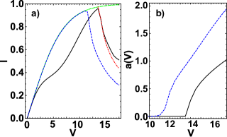
Figure 2: a) Current through the model spintromechanical transistor shown in Fig. 1 as a function of bias voltage for different dot oscillation frequencies. The current is normalized to the maximum (saturation) current of a device with an immobile quantum dot, $I_{m}=(e\Gamma/2\hbar)[4\Omega_{H}^{2}/(\Gamma^{2}+4\Omega_{H}^{2})]$ (see Ref. Zubov, ]; the bias voltage is measured in units of $\Gamma$. The solid (black on-line) curve corresponds to $\hbar\omega/\Gamma\simeq 0.15$ and the short-dashed curve (blue on-line) to $\hbar\omega=0.5\Gamma$. Curves for higher frequencies (e.g., $\hbar\omega=1.5\Gamma$) practically coincide with the short-dashed curve and are not shown. The dashed-dotted curve (red on-line) is the result of a simplified semi-analytical model calculation (see text) and the dashed curve (green on-line) is the $I-V$ curve for a device with an immobile quantum dot. The plots demonstrate that in contrast to what is the case for an ordinary single-electron transistor, the $I-V$ characteristics of a spintromechanical transistor are strongly nonlinear. b) The dependence of amplitude $a(V)$ of the developed shuttling oscillations (normalized to the tunneling length $\lambda$) on bias voltage normalized by $\Gamma$. The solid curve corresponds to $\hbar\omega/\Gamma\simeq 0.15$ and the short-dashed curve (blue on-line) to $\hbar\omega/\Gamma=0.5$. It is clearly seen from the plots that low- and high-voltage parts of $I-V$ curves in Fig.2(a) correspond to vibronic and shuttling regimes of electron transport. Other parameters used in numerical calculations are: the Coulomb correlation energy $U=0$, the level energy (counted from the Fermi energy) $\varepsilon_{0}/\Gamma=1$, magnetic field $\Omega_{H}/\Gamma=0.1$, temperature $T/\Gamma=1.5$, exchange coupling $J/\Gamma=0.77$, the electromechanical coupling constant $\kappa=\hbar^{2}/(m\lambda\lambda_{J}\Gamma)=0.06$, where $\kappa$ is the coefficient multiplying r.h.s. of Eq. (5) written in terms of dimensionless variables $x$ and $t$, and the distance between the leads is set to be $d=20\lambda$.

With a further increase of bias voltage the current decreases rapidly. The magnitude of the current drop is of the order of the maximum current. The two different regimes of electron transport are related to two different phases of the mechanical QD oscillations. In the low-bias regime the amplitude $a(V)$ of the QD oscillations is vanishingly small (vibronic phase). At the threshold bias voltage the amplitude starts to grow rapidly until it reaches a value of a few $\lambda$ (see Fig. 2(b), where the QD vibration amplitude $a(V)$ is normalized to the tunneling length $\lambda$). This is the shuttling regime of electron transport fedorets ; fedorets1 .

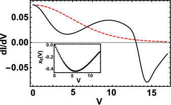
Figure 3: Differential conductance as a function of bias voltage. The solid (black on-line) curve corresponds to $\hbar\omega/\Gamma\simeq 0.15$ and the dashed (red on-line) curve is for an immobile quantum dot. The oscillation of magnetic shuttle introduces the negative differential conductance in $V\gtrsim 13$. The inset shows the exchange and electric force-induced shift of dot coordinate $x_{0}(V)$. Strongly non-linear dependence of $x_{0}(V)$ on bias voltage results in non-monotonic differential conductance. Other parameters used in numerical calculations are the same as in Fig. 2.

As mentioned in the Introduction, a rough estimate of the threshold bias voltage gives $eV_{th}\sim Jd/\lambda\simeq 16\,\Gamma$ (for $J=0.77\,\Gamma$ and $d/\lambda=20$, $\lambda=\lambda_{J}$). This is in a reasonably good agreement ($\sim 50\%$) with numerical results for the same parameters (see Fig. 2(a)). Notice, however, that the threshold voltage observed numerically depends on frequency (see Fig. 2(b)) and that this frequency dependence in the considered spintromechanical device looks qualitatively different from the one for shuttling of spinless electrons, in which case $eV_{th}\propto\hbar\omega$ (see Ref. fedorets, ). It is clear from Fig. 2(b) that $V_{th}(\omega_{1})\leq V_{th}(\omega_{2})$ for $\omega_{2}\leq\omega_{1}$. However, the effect is not numerically large since $\max(\delta V_{th}/V_{th})<0.2$.

Let us first explain the non-monotonic behavior of the differential conductance, $dI/dV$, in the vibronic ”phase“ of dot oscillations and focus on the adiabatic regime, where $\hbar\omega\ll\Gamma$ (see Fig. 3, where the red curve shows the voltage dependence of the differential conductance of a non-movable quantum dot as calculated using Eq. (A.20) of Ref. Zubov, ). For small magnetic fields, $h\equiv g\mu_{B}H\ll\Gamma$, the exchange force induces a shift, $x_{0}(V)<0$, of the quantum dot in the direction of the source electrode if the dot is occupied by a spin-up electron. This shift depends non-monotonically on the bias voltage (see the inset in Fig. 3) due to the different voltage-dependencies of the electric and magnetic forces. The electric force has a simple linear dependence on the bias voltage while the voltage dependence of the exchange force is more complicated. This is because it has an exponential dependence on the voltage dependent shift $x(V)$ of the dot, $\sim J\sinh x_{0}(V)$. In addition the exchange force depends on the voltage-dependent probability for the dot to be occupied by a spin-up electron, see Eq. (5).

At zero bias, $V=0$, the probabilities to fill the dot level with a spin-up electron from the source or a spin-down electron from the drain are equal, so there is no net exchange force on the dot (nor is there any electric force). A finite bias voltage favors spin-up states on the dot and therefore leads to an exchange force that acts to shift the dot towards the source electrode, a shift that itself increases the exchange force. The exchange force is opposed by the electric force, $\propto V$, and the elastic restoring force, $\propto\omega^{2}x_{0}(V)$, which leads to a voltage dependent shift $x_{0}(V)$ for which these forces balance each other. The shift has a maximum value for some finite voltage and decreases if the voltage is increased further as the electric force, which is always directed towards the drain electrode, grows in strength. When the electric force equals the magnetic force the dot returns to its symmetric position and there is no shift (see the inset in Fig. 3). (Note that in the vibronic phase at low frequencies this maximum shift is always smaller than the tunneling length $\lambda$, decreases with increasing $\omega$, and saturates at negligibly small values when $\hbar\omega\geq\Gamma$.) As a result, the differential conductance is a non-monotonic function of voltage. This is a special feature of a spintromechanical transistor in the adiabatic regime of dot oscillations. The effect disappears at high oscillation frequencies $\hbar\omega\geq\Gamma$ when the voltage-induced shift of the quantum dot is negligibly small and the $I-V$ characteristics coincide with the simple analytical dependence known for an immobile quantum dot Zubov .

Now we proceed to a discussion of the shuttling regime of transport. Electric shuttling starts in the vicinity of the threshold bias voltage for which the current almost reaches the maximum value that can be achieved in a symmetric junction. If we neglect small frequency-dependent variations in $V_{th}$, electric shuttling begins exactly at the point where the electric and magnetic forces compensate each other, the quantum dot is in its symmetrical position and the current is maximal. At these high voltages the dot level (in our simulations $\varepsilon_{0}=1\,\Gamma$) is populated by spin-up electrons with almost 100% probability. The magnetic force is compensated and there is no threshold for electric shuttling. Is there room for spin-induced effects in this regime of electron transport? To answer this question we consider a simple adiabatic model for shuttling, using the numerically evaluated dependence of the shuttling amplitude on bias voltage, see Fig. 2(b).

In Ref. Zubov, an analytic expression for the electric current in a spintronic transistor with an immobile quantum dot was derived (see Eq. (A.20) in the Appendix of the cited paper)

$$I=e\frac{\Gamma_{L}\Gamma_{R}}{\Gamma_{L}+\Gamma_{R}}\frac{h^{2}}{\Gamma_{L}\Gamma_{R}+h^{2}}(f_{L}^{+}-f_{R}^{+}).$$ (21)

Here $h=g\mu_{B}H$ and $2f^{\pm}_{L,R}=f_{L,R}(\varepsilon_{1})\pm f_{L,R}(\varepsilon_{2})$, $\varepsilon_{1,2}=\varepsilon_{0}\pm h/2$ are the Zeeman-split dot energy levels and $f_{j}(\varepsilon)$ is the Fermi distribution function characterized by chemical potential $\mu_{j}$ and temperature $T$. We generalize this simple model for our case by assuming that in the adiabatic regime of dot oscillations one can replace the tunneling couplings $\Gamma_{j}$ by the time-dependent quantities $\Gamma_{j}\{x(t)\}=\exp(\mp x(t)/\lambda)$, where $x(t)=a(V)\cos\omega t$ is the voltage-dependent amplitude of shuttle oscillations (see Fig. 2(b)). We include also the exchange-interaction-induced time-dependent gap in the level splitting $\delta\varepsilon=\sqrt{h^{2}+4J^{2}\sinh^{2}[x(t)/\lambda]}$ in order to take into account the effects of the exchange interaction. Now the time-dependent current takes the form (we omit the last factor in Eq.(21), which describes the effects of level populations; we numerically checked that this factor is very close to one and it does not modify the calculated $I-V$ characteristics in the shuttle regime of transport)

$$I_{m}(t)=\frac{e\Gamma}{2\hbar\cosh[x(t)/\lambda]}\frac{h^{2}}{\Gamma^{2}+h^{2}+4J^{2}\sinh^{2}[x(t)/\lambda]}.$$ (22)

This current depends on bias voltage through the voltage-dependent amplitude $a(V)$ of shuttling, Fig. 2(b). The current Eq. (22) averaged over one period of oscillation $2\pi/\omega$ results in the desired current-voltage characteristics $\bar{I}(V)$ plotted in Fig. 2(a) (dashed-dotted curve, red on-line) for the case of a low frequency $\hbar\omega\simeq 0.15\,\Gamma$.

We note the good agreement, obvious from Fig. 2(a), between the full numerical solution and the result of our simple adiabatic model. More importantly, however, we can use the analytical model to reveal physical effects hidden in the numerically obtained $I-V$ curves. The two factors in Eq. (22) describe two different effects that result in a reduction of the current (and in a negative differential conductance) in our spintromechanical transistor. The first factor in Eq. (22), when averaged over time, describes the current suppression that originates from the increased contact resistance of an effectively non-symmetric tunnel junction. It has nothing to do with spin effects in our magnetic device. The second term appears due to spin-flips in the external magnetic field. We see that the appearance of a voltage-dependent gap in the Rabi-oscillations between spin-up and spin-down states could strongly suppress the averaged current. For the parameters used in our calculations the two factors contribute almost equally to the current drop. This means that the spin-polaronic effects (see also Ref. pulkin, ) are significant in the electric shuttling regime in magnetic spintromechanical transistors. Note that the time-averaged current $\bar{I}(V)$ depends on frequency $\omega$ through the frequency dependence of the shuttling amplitude, which can be evaluated numerically, see Fig. 2(b). We have compared $I-V$ curves calculated by using the adiabatic model with full numerical results for $\hbar\omega=0.5\,\Gamma$ and $1.5\,\Gamma$ and found agreement within an accuracy of a few per cent (the comparison for $\hbar\omega=0.5\,\Gamma$ as well as the curves for $\hbar\omega=1.5\,\Gamma$ are not presented in Fig. 2(a) in order not to overload the figure with plots).

The last question we want to discuss here is: How do electron-electron correlations influence the $I-V$ characteristics in the transport regime where the Coulomb blockade is not pronounced? Figure 4 shows numerical results for a Coulomb energy of $U=4.5\,\Gamma$. All other model parameters are essentially the same as those used for the case of noninteracting electrons (note the different normalization current, $e\Gamma/(2\hbar)$, as compared to Fig. 2(a)). We see that all spin effects discussed earlier for noninteracting electrons survive when the Coulomb interaction is turned on. There is no qualitative change in the current-voltage dependencies. The only new effect is the appearance of a small negative differential conductance for the case of an immobile quantum dot (see Ref. gorelik, ).

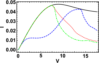
Figure 4: The $I-V$ curves of spintromechanical transistor for a Coulomb energy $U=4.5\,\Gamma$. Other parameters used in numerical calculations are: the level energy (counted from the Fermi energy) $\varepsilon_{0}/\Gamma=1$, magnetic field $\Omega_{H}/\Gamma=0.1$, temperature $T/\Gamma=1.5$, exchange coupling $J/\Gamma\simeq 0.8$, the electromechanical coupling constant $\kappa=0.06$ and the distance between the leads is set to be $d=20\lambda$. Note that the current is normalized to $(e\Gamma)/(2\hbar)$. The dashed curve (blue on-line) corresponds to $\hbar\omega/\Gamma\simeq 0.16$, the short-dashed curve (red on-line) - $\hbar\omega/\Gamma=0.5$, the dashed-dotted curve (green on-line) - $\hbar\omega/\Gamma=1.5$ and the solid curve (black on-line) represents current-voltage dependence for the spintronic device with a non-movable quantum dot.

In summary, we have shown that spin-polaronic effects give rise to special features in the current-voltage characteristics of a spintromechanical magnetic transistor even in the case when exchange forces do not lead to magnetic shuttling. Both the low-voltage (vibronic) and the high-voltage (electric shuttling) phases demonstrate unusual behavior, which is characterized by a differential conductance with a non-monotonic voltage dependence (vibronic phase) and a negative differential conductance (electric shuttling phase). We predict that the appearance of a negative differential conductance can be used as a signature of shuttling in spintromechanical magnetic devices.

Acknowledgement. This work was supported by the Institute for Basic Science in Korea (IBS-R024-D1); the National Academy of Sciences of Ukraine (grant No. 4/19-N and Scientific Program 1.4.10.26.4); the Croatian Science Foundation, project IP-2016-06-2289, and by the QuantiXLie Centre of Excellence, a project cofinanced by the Croatian Government and the European Union through the European Regional Development Fund - the Competitiveness and Cohesion Operational Programme (Grant KK.01.1.1.01.0004). The authors acknowledge the hospitality of PCS IBS in Daejeon (Korea). OAI thanks V.V. Slavin and Y.V. Savin for the help in organization of computer calculations.

References

- (1) R. Hansen, L.P. Kouwenhoven, J.R. Petta, S. Tarucha, and L.M.K. Vandersypen, Rev. Mod. Phys. 79, 1217 (2007).
- (2) K.C. Novak, F.H.L. Koppens, Yu.V. Nazarov, and L.M.K. Vandersypen, Science 318, 1430 (2007).
- (3) S. Foletti, H. Bluhm, D. Mahalu, V. Umansky, and A. Yacoby, Nat. Phys. 5, 903 (2009).
- (4) F. Jelezko, T. Gaebel, I. Popa, A. Gruber, and J. Wrachtrup, Phys. Rev. Lett. 92, 076401 (2004).
- (5) D. Press, T.D. Ladd, B. Zhang, and Y. Yamamoto, Nature 456, 218 (2008).
- (6) L.Y. Gorelik, D. Fedorets, R.I. Shekhter, and M. Jonson, New J. Phys. 7, 242 (2005).
- (7) L.Y. Gorelik, A. Isacsson, M.V. Voinova, B. Kasemo, R.I. Shekhter, and M. Jonson, Phys. Rev. Lett. 80, 4526 (1998).
- (8) A. Erbe, C. Weiss, C.W. Zwerger, and R.H. Blick, Phys. Rev. Lett. 87, 096106 (2001).
- (9) D.R. Koenig and E.M. Weig, Appl. Phys. Lett. 101, 213111 (2012).
- (10) Chulki Kim, Marta Prada, Gloria Platero, and Robert H. Blick, Phys. Rev. Lett. 111, 197202 (2013).
- (11) S.I. Kulinich, L.Y. Gorelik, A.N. Kalinenko, I.V. Krive, R.I. Shekhter, Y.W. Park, and M. Jonson, Phys. Rev. Lett. 112, 117206 (2014).
- (12) D. Fedorets, L.Y. Gorelik, R.I. Shekhter, and M. Jonson, Europhys. Lett. 58, 99 (2002).
- (13) O.A. Ilinskaya, S.I. Kulinich, I.V. Krive, R.I. Shekhter, H.C. Park, and M. Jonson, New J. Phys. 20, 063036 (2018).
- (14) O.A. Ilinskaya, D. Radic, H.C. Park, I.V. Krive, R.I. Shekhter, and M. Jonson, Phys. Rev. B 100, 045480 (2019).
- (15) O.A. Ilinskaya, A.D. Shkop, D. Radic, H.C. Park, I.V. Krive, R.I. Shekhter, and M. Jonson, Low Temp. Phys. 45, 1032 (2019).
- (16) T. Novotny, A. Donarini, and A.-P. Jauho, Phys. Rev. Lett. 90, 256801 (2003).
- (17) Yu.D. Zubov, O.A. Ilinskaya, I.V. Krive, and A.A. Krokhin, J. Phys.: Condens. Matter 30, 315303 (2018).
- (18) R.I. Shekhter, A. Pulkin, M. Jonson, Phys. Rev. B 86, 100404 (2012).
- (19) L.Y. Gorelik, S.I. Kulinich, R.I. Shekhter, M. Jonson, and V.M. Vinokur, Phys. Rev. Lett. 95, 116806 (2005).