How to Choose the Most Appropriate Centrality Measure? A Decision Tree Approach

Abstract

Centrality metrics play a crucial role in network analysis, while the choice of specific measures significantly influences the accuracy of conclusions as each measure represents a unique concept of node importance. Among over 400 proposed indices, selecting the most suitable ones for specific applications remains a challenge. Existing approaches—model-based, data-driven, and axiomatic—have limitations, requiring association with models, training datasets, or restrictive axioms for each specific application. To address this, we introduce the culling method, which relies on the expert concept of centrality behavior on simple graphs. The culling method involves forming a set of candidate measures, generating a list of as small graphs as possible needed to distinguish the measures from each other, constructing a decision-tree survey, and identifying the measure consistent with the expert’s concept. We apply this approach to a diverse set of 40 centralities, including novel kernel-based indices, and combine it with the axiomatic approach. Remarkably, only 13 small 1-trees are sufficient to separate all 40 measures, even for pairs of closely related ones. By adopting simple ordinal axioms like Self-consistency or Bridge axiom, the set of measures can be drastically reduced making the culling survey short. Applying the culling method provides insightful findings on some centrality indices, such as PageRank, Bridging, and dissimilarity-based Eigencentrality measures, among others. The proposed approach offers a cost-effective solution in terms of labor and time, complementing existing methods for measure selection, and providing deeper insights into the underlying mechanisms of centrality measures.

I Introduction

Understanding networks relies heavily on centrality metrics. However, the vast number of proposed point centrality measures, which now exceeds 400 and continues to grow [1] (cf. [2, 3, 4]), poses a challenge when it comes to selecting the most appropriate centrality indices for specific applications.

In some cases, researchers have a mathematical model that accurately captures the influence of nodes in the process of interest, naturally suggesting a measure of node importance that can be interpreted as centrality [5, 6, 7, 8, 9, 10, 11].

However, in many cases, no detailed model is available, while the centrality of network nodes needs to be estimated. To address this, researchers rely on studying the typology of the application and theoretical taxonomy of centrality indices [6, 2, 3, 12, 13, 4, 14] to narrow down the options. Further, specific measures can be compared experimentally by studying correlations, regressions, and appropriate distances between them and external network characteristics [15, 16, 17, 2, 18, 19, 20, 21, 14] and (or) using Principal Components Analysis (PCA) [12, 22]. On the other hand, such studies yield varying results across datasets within the same subject area [23] and do not uncover the underlying causes of correlations.

Hence, to supplement the experimental perspective, it is essential to focus on the properties of centralities and the conditions they satisfy. The quintessence of this is the axiomatic approach, which seeks to characterize a measure by a minimal set of axioms it uniquely satisfies (we refer to [24, 25, 26, 27, 28, 29, 30] for several examples). In [14], typology is incorporated into this approach by the use of nodal statistics.

However, the axiomatic approach has its limitations. Some of them are as follows.

1. Only a minority of measures are axiomatized, since constructing a suitable set of axioms is a non-trivial task.

2. For parametric families of measures (such as those in [31, 32, 33]), selecting the parameter value rarely has an axiomatic solution.

3. In many axiomatics, there is at least one technical axiom, which is not appealing in itself and rather specifies the functional form of a centrality (see, e.g., Closeness, Degree, and Decay axioms in [27], Linearity in [28], Neighbor separability in [34]). It can be argued that adopting such an axiom does not fundamentally differ from adopting a measure at once.

4. Some non-technical axioms have rather sophisticated formulations, which makes it difficult to assess their desirability.

5. Comparing multiple axiomatics can be laborious, with no guarantee of reaching a definitive choice among them.

6. The rankings of nodes in simple networks provided by a measure satisfying a set of axioms may be counterintuitive to users, despite the initial appeal of the axioms.

For example, the Weighted degree centrality [35]

$$f(u)=\sum_{v\in V,\,v\neq u}\frac{D(v)}{d(u,v)},$$

where $V$ is the node set of a graph $G,$ $D(v)$ is the degree of node $v$, $d(u,v)$ being the shortest path distance between $u$ and $v,$ implements the reasonable idea of measuring the centrality of $u$ by the sum of the degrees of all other nodes with weights decreasing with distance from $u.$ This measure satisfies four out of six axioms considered in [35] (while Betweenness or Eigenvector centrality satisfy three axioms and no measure under study satisfies five or six) and its characterization is likely to be obtained by adding a suitable axiom of an algebraic nature. However, for any star (a graph with $n>2$ nodes and $n-1$ edges incident to the same node called the center), this index considers the center to be less central than the leaves. It follows that $(i)$ the Weighted degree measures something other than centrality; $(ii)$ the performance of a measure on simple examples is no less informative than the underlying heuristics or axioms it satisfies.

The main observation that prompted this study was that professionals familiar with a particular application often rely on their experience (frequently based on objective results) to compare node centrality in simple networks. In this case, we can select a centrality measure that ranks the nodes in the same way. Furthermore, such a centrality can be sought in the set of measures that satisfy the axioms that the expert considers important.

As another instructive example, consider the PageRank centrality [36, 37, 38], which was originally proposed for directed reference networks (see [39, 5]) and has axiomatizations [40, 30]. Note that it sets $f(4)>f(5)$ (node 4 is more central than node 5) for the graph $G_{5}$ in Fig. 1. As well as some other inequalities it produces (namely, $f(4)>f(0)$ for $G_{2}$; $f(1)>f(0)$ for $G_{7}$; $f(0)>f(2)$ and $f(1)>f(5)$ for $G_{9}$), this seems rather counterintuitive. On the other hand, an analysis of the mechanism of this centrality reveals [41] some types of real-world undirected networks that may require such a measure. This kind of singularity of measures may go unnoticed in an axiomatic study, but it is easy to detect when centralities are tested on a set of specially selected graphs.

Taking into account the above limitations of the axiomatic strategy, in this paper we propose an alternative approach based on expert beliefs on how the desired centrality should act on test graphs.

Purpose of the Study

We consider centrality measures on undirected graphs. Given a graph $G=(V,E)$ with node set $V=V(G)$ such that $|V(G)|>3$ and edge set $E=E(G)$, a centrality measure $f$ associates a real number $f(v)$ to each node $v\in V(G)$. This number is interpreted as follows: the larger $f(v),$ the more central $v$ is considered. While $f(v)$ depends on $G,$ for simplicity we do not reflect this in the notation as only one graph is considered at a time. We confine ourselves to connected graphs, since there are centralities defined only for them. Let ${\cal F}=\{f_{1},\ldots,f_{m}\}$ be a set of centrality measures, and each $f_{i}$ is applicable to any graph of the above type.

In this paper, we are mainly interested in the order of centrality values, not the numerical values themselves. Let us say that a graph $G$ distinguishes $($or separates$)$ measures $f_{i}$ and $f_{j}$ on a pair of nodes $\{u,v\}$ $(u,v\in V(G))$ whenever

$$\mathop{\rm sign}\nolimits(f_{i}(u)-f_{i}(v))\neq\mathop{\rm sign}\nolimits(f_{j}(u)-f_{j}(v)).$$ (1)

In words (1) means that $f_{i}$ and $f_{j}$ disagree in comparing the centrality of $u$ and $v.$

Centrality measures $f_{i}$ and $f_{j}$ are rank equivalent if and only if there exists no graph that distinguishes them. We suppose that no distinct measures in ${\cal F}$ are rank equivalent. Eliminating rank equivalent “twins” of some measures can be done by considering a large enough series of large enough graphs: if no graph distinguishes a couple of measures, we remove one of them, even if we have not been able to rigorously prove that they are rank equivalent.

The aim of this work is to propose a method that allows the expert to select a centrality measure that matches their application-specific understanding of how such a measure should act on a collection of test graphs.

Given a set of measures ${\cal F}$, we need to construct:

• a collection of fairly simple graphs that contains a distinguishing graph for every pair of distinct measures $f_{i},f_{j}\in{\cal F};$

• a questionnaire such that every set of responses to its questions determines a unique measure.

Ideally, these collection and questionnaire should be generated and modified automatically whenever a new set ${\cal F}$ is provided or an existing set ${\cal F}$ is updated.

The method that consists in constructing such collections and questionnaires and passing the corresponding surveys to select the most appropriate centrality measures will be called culling. We develop this method in the following section. The computer code that implements it is provided at https://github.com/DAGubanov/centralities_dec_tree.

II Results

We now present the main procedures of the culling method and then illustrate its application.

II-A Generating Graphs that Distinguish Measures

Let a set ${\cal F}$ of rank-nonequivalent centrality measures be given. We aim to construct a list ${\cal G}=(G_{1},\ldots,G_{K})$ of graphs that separate all measures in ${\cal F}.$

The distinguishing graphs should be simple enough for experts to answer which pairwise centrality order, i.e., $f(u)>f(v)$ or $f(u)<f(v)$ or $f(u)=f(v)$ is most consistent with their application-specific understanding based on their experience and previous studies.

For our first survey, we opted for the class of unicyclic graphs (also called unicycles, $1$-trees, or augmented trees). These are connected graphs with the number of edges equal to the number of nodes. Such a graph can be obtained from a tree by connecting any two non-adjacent nodes with an edge.

The advantage of $1$-trees is that they are simple and can be even more comfortable to perceive and compare the centrality of nodes than trees, thanks to an eye-catching cycle (Fig. 1).

The procedure of constructing the list ${\cal G}=(G_{1},\ldots,G_{K})$ of separating $1$-trees is as follows.

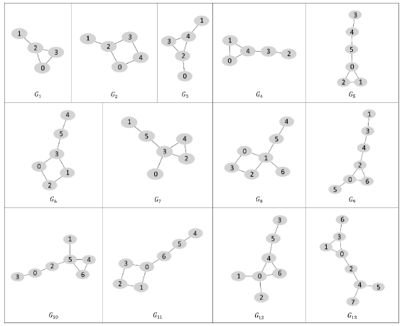
Figure 1: Distinguishing graphs for the test set ${{\cal F}^{40}}$ of 40 centrality measures.

1. At the beginning, the list ${\cal G}$ is empty.

2. We sequentially generate unlabeled trees, starting from the trees with four nodes and increasing the number of nodes.

   1. For each tree, we produce various $1$-trees by adding different edges that connect non-adjacent nodes.

      1. For each unlabeled $1$-tree $G$, we look for the couples $f_{i},f_{j}\in{\cal F}$ such that the current list ${\cal G}$ (let $|{\cal G}|=k$) still contains no graph that separates $f_{i}$ and $f_{j},$ while $G$ separates them on some pair $\{u,v\}$ of its nodes.

         1. If $\{f_{i},f_{j}\}$ is such a couple, then we add $G$ to the list ${\cal G}$ as $G_{k+1}$ and associate a separating triple $(G_{k+1},u,v)$ with $\{f_{i},f_{j}\}$.

3. We stop the generation process when a separating triple $(G_{k+1},u,v)$ is associated with every pair of distinct centrality measures in ${\cal F}$.

This simple procedure was sufficient to separate all measures in the set ${{\cal F}^{40}}$ of $40$ centralities (see Section II-D) by means of $13$ $1$-trees with at most $8$ nodes. Among them, there are five graphs with $7$ nodes and only one with $8$ nodes. Therefore, the “separating power” of $1$-trees on $8$ nodes is far from exhausted and can potentially separate a much larger number of measures. Moreover, for our test survey we limited ourselves to $1$-trees with node degrees at most four, which is not obligatory in the above procedure.

However, there is no guarantee that all couples of different measures in ${\cal F}$ can be separated by $1$-trees. To guarantee a complete separation, we propose the following general procedure that iterates over the entire set of connected graphs. It includes the above procedure as the first stage to make the most of $1$-trees.

1. At the beginning, the list ${\cal G}$ is empty.

2. Increase $n$ starting with $3,$ and while there are unseparated measures in ${\cal F}$ and $n\leq 8,$ sequentially use all connected graphs with $n$ nodes and $n$ edges ($1$-trees) to separate measures in ${\cal F}$ as in the previous procedure.

3. If there are still unseparated measures in ${\cal F}$, proceed as in Item 2 with trees (i.e., with connected graphs having $n-1$ edges).

4. If there are still unseparated measures in ${\cal F}$, proceed as in Item 2 with connected graphs having $n+1$ edges.

5. Continue in the following way until all measures in ${\cal F}$ are separated:

   1. For each increasing $n>8$ :

      1. Sequentially use, to separate the not yet separated measures in ${\cal F},$ all connected graphs with $n$ nodes and: (a) $n$ edges ($1$-trees); (b) $n-1$ edges (trees); (c) $n+1$ to $2n-8$ edges;

      2. Generate and use: (d) all connected graphs with $n^{\prime}\leq n$ nodes and $n^{\prime}+n-7$ edges, starting with the smallest $n^{\prime}$ allowing that many edges and increasing $n^{\prime}.$

In this general procedure, with each incremented $n>8$, we increase the maximum difference between the number of edges and nodes to $(n^{\prime}+n-7)-n^{\prime}=n-7$ (see (d) in 5.1.2 above) and check all graphs with this difference and the number of nodes at most $n.$ This maximum difference grows slowly to keep the test graphs simple enough by keeping their density as low as possible.

The next task is constructing a questionnaire that allows the expert to choose the centrality measure that suits them best.

II-B Constructing a Decision Tree

We now present a procedure for constructing a questionnaire, which takes the form of a decision tree.

In every next question, the expert is asked to compare the centrality of two nodes $u$ and $v$ in some graph $G_{k}\in{\cal G}.$ This graph separates certain measures that match all the expert’s responses already received. The new response is $f(u)>f(v),$ or $f(u)<f(v),$ or $f(u)=f(v)$ and it narrows down the set of suitable measures keeping only those $f_{i}\in{\cal F}$ for which this response is correct. The survey continues until only one measure remains.

Thus the questions in the survey depend on the responses to the previous ones. Therefore, the questionnaire has the structure of a rooted directed tree. The expert navigates the tree answering the questions associated with the root and intermediate vertices. Each answer is identified with an arc directed from the vertex corresponding to the question. The leaves, i.e., the vertices of the tree that have no outgoing arcs, are identified with the measures.

We now present a procedure for constructing such a tree. Let us have a set ${\cal F}$ ($|{\cal F}|>1$) of centrality measures and a list of distinguishing graphs ${\cal G}=(G_{1},\ldots,G_{K}).$ For each couple of distinct measures $f_{i},f_{j}\in{\cal F},$ a triple $(G_{k},u,v)$ is associated with this couple such that $G_{k}\in{\cal G}$ separates $f_{i}$ and $f_{j}$ on the pair $\{u,v\}$ of its nodes.

At the initial step of the procedure, we are at the root of the tree. There are no other vertices in the tree yet, and no question is associated with the root.

On each step of the procedure, we are at some vertex $x$ of the tree. A standard step of the procedure is any step, except for “finish.”

The standard step consists of the following.

• Consider the path from the root to $x.$ Each arc of this path corresponds to some condition: it is a response to the question associated with the vertex this arc is directed from. Let ${\cal F}_{x}\subseteq{\cal F}$ be the set of measures satisfying all conditions in this path (if $x$ is the root, then ${\cal F}_{x}={\cal F}$).

• If no question has yet been associated with $x$ and ${|{\cal F}_{x}|>1}$, then take $G_{k}\in{\cal G}$ with the smallest $k$ such that $G_{k}$ separates some measures in ${\cal F}_{x}$ on a certain pair of its nodes $\{u,v\}.$ Choose a suitable pair $\{u,v\}$ arbitrarily and associate the question “What inequality (equality) holds true for $f(u)$ and $f(v)$ in $G_{k}$?” with $x.$ Draw two or three arcs directed from $x$ to newly created vertices, depending on which of the three conditions $f(u)>f(v),$ $f(u)<f(v),$ or $f(u)=f(v)$ are met by the measures in ${\cal F}_{x}.$ Assign the conditions that can be satisfied by the measures in ${\cal F}_{x}$ to these arcs. Mark these arcs as “new.”

• If there is at least one “new” arc directed from $x,$ choose any such arc, move to the vertex this arc is directed to, and mark this arc as “old.”

• If $|{\cal F}_{x}|=1,$ then associate with $x$ the unique centrality measure that belongs to ${\cal F}_{x}.$

• If (a) there is no “new” arc directed from $x,$ while there is a question associated with $x,$ and $x$ is not the tree root or (b) $|{\cal F}_{x}|=1,$ then make one move back from $x$ toward the root.

• If there is no “new” arc directed from $x,$ while there is a question associated with $x$ and $x$ is the root, then finish: the decision tree is built. Otherwise, make another standard step from $x.$

A high-level pseudocode of the standard step is given in Algorithm 1.

Algorithm 1 Recursive Construction of a Decision Tree.

Input: $\mathcal{F}$, a set of centrality measures; $\mathcal{G}=(G_{1},\dots,G_{K})$, a list of distinguishing graphs; a set of distinguishing triples of the form $(G_{k},u,v)$.

Result: Decision tree for choosing a centrality measure

procedure standardStep($x$)

     if $|\mathcal{F}_{x}|>1$ then

         $(G_{k},u,v)\leftarrow\text{distinguishMeasures}(\mathcal{F}_{x})$

         $x.\text{associateQuestion}(\text{``$f(u)$ vs $f(v)$ in $G_{k}$''})$

         $x.\text{addNewArcsAndChilds}(G_{k},u,v)$

         while $x.\text{hasNewArcs()}$ do

              $arc\leftarrow x.\text{getAnyNewArc()}$

              $\text{markArcAsOld}(arc)$

              $\text{standardStep}(arc.target)$          

     else

         $x.\text{associateUniqueMeasure}(\mathcal{F}_{x})$      

II-C Extending a Decision Tree

Suppose now that several new centrality measures (for example, recently appeared in the literature) are added to an existing set ${\cal F}$. Should we rebuild the decision tree from the beginning? The answer is no.

First consider the simplest case where only one measure $f^{\prime}$ is added. There are two possibilities:

• the new measure $f^{\prime}$ satisfies the same set of conditions (answers to the questions of the current decision tree) as one of the “old” measures;

• in the current decision tree applied to the extended set ${\cal F}^{\prime}={\cal F}\cup\{f^{\prime}\},$ there is a vertex $x$ such that $f^{\prime}\in{\cal F}^{\prime}_{x},$ but only two arcs are directed from $x,$ while the third possible answer to the question associated with $x$ is correct for $f^{\prime}.$

In case (b), it remains to add a third arc directed from $x,$ i.e., attach the third possible answer to the question associated with $x,$ after which an updated tree is built.

In case (a), we need to distinguish $f^{\prime}$ from an “old” measure $f_{i}$ that satisfies the same set of conditions. Since $f_{i}$ and $f^{\prime}$ end up on the same leaf of the current decision tree, we need to make this leaf an intermediate vertex by associating a new question with it. To formulate this question, we first check if ${\cal G}$ contains a graph that separates $f_{i}$ and $f^{\prime}$ on some pair of its nodes $\{u,v\}.$ If such a graph $G$ exists, then the required question is: “Which inequality (or equality) is true for $f(u)$ and $f(v)$ in $G$?” Otherwise, we need a new graph that separates $f_{i}$ and $f^{\prime},$ so we call the graph generation procedure described in Section II-A for the set of measures $\{f_{i},f^{\prime}\}$.

Thus, adding a new measure $f^{\prime}$ leads to the addition of /either a question or a possible answer to an existing question. So the total number of questions in the questionnaire does not exceed $m-1,$ where $m$ is the number of measures. If three arcs are directed from $k$ vertices of the tree, then the number of questions is obviously $m-k-1.$

Suppose now that several measures have been added to ${\cal F}.$ Then we need the following:

1. For each new measure $f^{\prime},$ check the above condition (b); if it is satisfied, then add the lacking arc to the decision tree;

2. Attach the new measures for which condition (b) is violated to the existing leaves of the tree, as for the above case (a);

3. Check whether ${\cal G}$ contains graphs that separate the measures associated with the same leaf and add the separating questions whenever such graphs exist;

4. For the couples of measures that cannot be distinguished by any graphs in ${\cal G},$ generate new graphs as described in Section II-A and add the required questions.

The above procedures of the culling method allow one to build a decision tree for selecting the most appropriate centralities for any set of measures ${\cal F}.$

II-D Test Survey

In Materials and Methods, we present several parametric classes of centralities based on similarity/dissimilarity measures for network nodes. Representatives of these classes are included in the set ${{\cal F}^{40}}$ designed to test the culling method. This set consists of the centralities listed in Table I.

TABLE I: The test set ${{\cal F}^{40}}$ of centrality measures

1. Betweenness​[42]	21. Bonacich​[43]
2. Closeness​[44]	22. Total communicability​[45]
3. Connectivity​[46]	23. Communicability $(K_{ij})$​[47]
4. Connectedness power​[34] ​​​​​​​​​​	24. Walk $(K_{ij})$​[48]
5. Degree​[44]	25. Walk $(K_{ii})$​[48]
6. Coreness​[49]	26. Estrada​[47]
7. Bridging​[50]	27. Eigencentrality (Dice dissimilarity​[51])
8. PageRank​[36]	28. Eigencentrality (Jaccard dissimilar.​[51])
9. Harmonic closeness​[52]	29. Closeness (Forest​[53])
10. Eccentricity​[44]	30. Closeness (Heat​[54])
11. $p$-Means $(p=-2)$​[33]	31. Closeness (logarithmic Forest​[55])
12. $p$-Means $(p=0)$​[33]	32. Closeness (logarithmic Walk​[56])
13. $p$-Means $(p=2)$​[33]	33. Closeness (logarithmic Heat​[54])
14. Beta current flow​[57]	34. Closeness (log-Communicability​[58])
15. Weighted degree​[35]	35. Eccentricity (Forest​[53])
16. Decaying degree​[35]	36. Eccentricity (Heat​[54])
17. Decay​[59]	37. Eccentricity (logarithmic Forest​[55])
18. Generalized degree​[32]	38. Eccentricity (logarithmic Walk​[56])
19. Katz​[48]	39. Eccentricity (logarithmic Heat​[54])
20. Eigenvector​[60]	40. Eccentricity (log-Communicability​[58])

The set ${{\cal F}^{40}}$ contains several pairs of closely related centralities. We include them to check whether they can be separated by sufficiently small low-density graphs, or whether large or dense graphs are necessary for this purpose.

The list ${\cal G}$ of distinguishing graphs generated for ${{\cal F}^{40}}$ consists of $13$ $1$-trees shown in Fig. 1. The culling decision tree involves $33$ questions in total. The length of a particular survey ranges from 1 to 12, with an average of $6.6$.

The survey begins with the question about the centrality of nodes 1 and 2 in $G_{1}$ (Fig. 2).

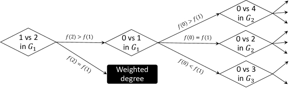
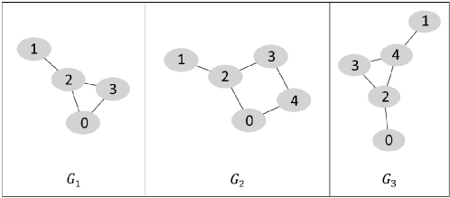
Figure 2: The beginning of the decision tree for the test set ${{\cal F}^{40}}.$

If the expert chooses $f(2)>f(1),$ then the second question concerns the centrality of nodes 0 and 1 in the same graph. If the answer is $f(0)>f(1),$ then the third question is about the centrality of nodes 0 and 4 in $G_{2}$. Otherwise, the expert who chooses $f(0)=f(1)$ is asked to compare $f(0)$ and $f(2)$ in $G_{2},$ whereas in the case of answer $f(0)<f(1),$ the third question is about the centrality of nodes 0 and 3 in $G_{3}$. If the expert chooses $f(2)=f(1)$ for the first question, then the survey ends yielding the Weighted degree [35] centrality.

The beginning of the survey is represented by the tree of Fig. 2. The whole tree is shown in Fig. 3 and Fig. 4.

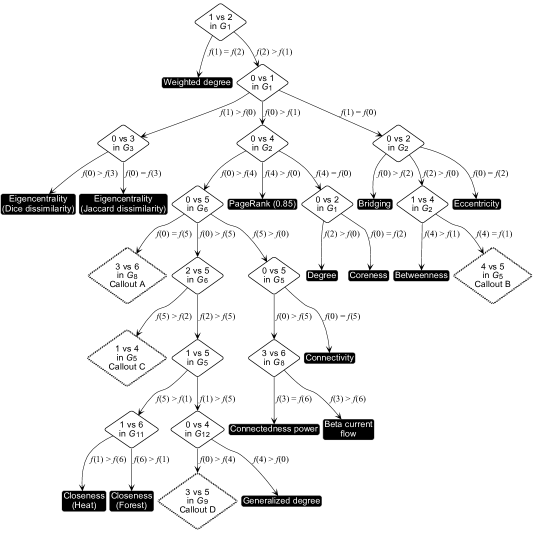
Figure 3: The decision tree for the test set ${{\cal F}^{40}}$; the callouts A to D are shown in Fig. 4.

   

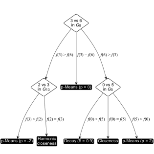
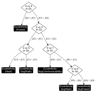
Callout A                                                  Callout B

   

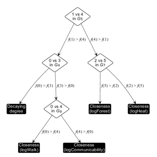
Callout C                                                  Callout D

Figure 4: Callouts A to D in Fig. 3.

The corresponding survey is implemented using Google Forms [61]. It allows everyone to choose from ${{\cal F}^{40}}$ the measure that best suits their concept of centrality. Each survey form (one of which is shown in Fig. 5) contains the instruction: “Choose the answer that best matches your feelings or your professional judgment… It would be optimal if you consider your specific application when choosing an answer.”

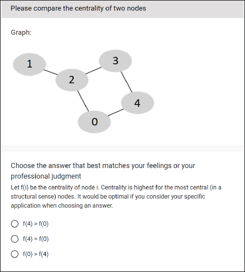
Figure 5: A sample survey form in [61].

Of particular interest will be the statistics of measure selection by a significant number of experts. The leaders of the early limited statistics are Degree, Closeness (Heat), and Closeness (logarithmic Forest).

Note that a decision tree for the entire set of known centralities can be built by extending the tree (or, in other terminology, the dendrogram) presented in Figures 3 and 4.

II-E Combination with the Axiomatic Approach

It can be seen that some questions in the above test survey are quite simple. Say, comparison of the centrality of nodes 1 and 2 in $G_{1}$ (Fig. 2) should be clearly in favor of 2. Therefore, the first question along with the Weighted degree index assigning equal centrality to nodes 1 and 2 can be eliminated, which reduces the number of questions in each survey by one.

The second question on the comparison of $f(0)$ and $f(1)$ in $G_{1}$ is less obvious, but also fairly simple. Indeed, the answer $f(0)<f(1)$ is unlikely to be popular, and most experts would probably choose $f(0)>f(1).$ Based on this, the Eigencentrality measures based on Dice dissimilarity and Jaccard dissimilarity can be eliminated as they suggest $f(0)<f(1).$ The answer $f(0)=f(1)$ may have some basis and ${{\cal F}^{40}}$ contains nine centralities that match it. These are the well-known Bridging and Betweenness measures and also the Eccentricity measures based on the Shortest path, Forest, Heat, logarithmic Forest, logarithmic Heat, logarithmic Walk, and logarithmic Communicability proximities. The decision tree of Fig. 3 makes the expert realize that choosing either of them implies adopting that nodes 0 and 1 in $G_{1}$ are equally central. Furthermore, the subsequent question (comparing nodes 0 and 2 in $G_{2}$) reveals that Bridging states that $f(0)>f(2),$ which is not very easy to accept; $f(0)=f(2)$ leads to Eccentricity; the remaining seven measures on this branch of the tree suggest $f(0)<f(2).$

Presumably the most popular answer, $f(0)>f(1),$ to the second question is followed by the comparison of $f(0)$ and $f(4)$ in $G_{2}.$ The rather specific answer $f(0)<f(4)$ leads to the PageRank measure (its peculiarities, which occur for all $\alpha\in\,(0;1)$, were discussed in Section I and in more detail in [41]), $f(0)=f(4)$ to Degree and Coreness, while $f(0)>f(4)$ to the remaining 25 measures on this branch of the tree.

The presence of questions, the answer to which is prompted by common sense or an application-specific understanding, suggests the formulation of the corresponding properties of centrality measures in the form of normative conditions (axioms). If the expert deems some of them necessary, this can drastically reduce the set of measures to be compared (cf. [62]). Based on this, we can offer the expert an abbreviated survey on the corresponding reduced set ${\cal F}^{\prime}\subset{\cal F}.$

This leads to a combination of culling with the axiomatic approach. In the next section, we discuss two conditions that can be used in this combination.

II-F Abbreviated Surveys

Among the axioms used in the literature to characterize centrality measures, the ones that are particularly appealing are those based on ordinal conditions. These axioms allow us to compare the centrality of certain nodes, but they do not provide explicit guidelines on how to calculate centrality in the general case.

Let us consider two such axioms and show how they can help significantly reduce the culling survey.

First, one may believe that the vector of centrality values of the neighbors (adjacent nodes) of any node $u$ carries a lot of information about the centrality of $u$ itself (cf. Consistency in [28]). A refinement of this requirement is that the greater the centrality values of the neighbors of a node, the greater the centrality of the node itself.

The following axiom is based on this idea. In the case of directed graphs, it appeared in [63]; for undirected graphs, in [35, 64] under the name of Structural consistency.

Let $N_{u}$ denote the set of neighbors of node $u$ in $G.$

Self-consistent monotonicity.  ​​If for $u,v\in V,$ there is an injection from $N_{u}$ to $N_{v}$ such that every element of $N_{u}$ is, according to $f(\cdot),$ no more central than the corresponding element of $N_{v}$, then $f(u)\leq f(v).$ If, additionally, $|N_{u}|<|N_{v}|$ or “no more” is actually “less” at least once, then $f(u)<f(v).$

For the subsequent analysis, we choose the following weaker and simpler axiom (cf. [65]).

Self-consistency.  ​​If for $u,v\in V,$ there exists a bijection between $N_{u}$ and $N_{v}$ such that each element of $N_{u}$ is, according to $f(\cdot),$ no more central than the corresponding element of $N_{v}$, then $f(u)\leq f(v).$ If “no more” is actually “less” at least once, then $f(u)<f(v).$

The idea of another axiom [29] is quite different. It allows to compare the centrality of two endpoints of a bridge. Recall that we consider centralities defined for all connected graphs $G$ with $|V(G)|>3.$

Bridge axiom.  ​​If the removal of edge $\{u,v\}$ from $E(G)$ separates $G$ into two connected components with node sets denoted by $V_{u}\ni u$ and $V_{v}\ni v$ (i.e., $\{u,v\}$ is a bridge), then $|V_{u}|<|V_{v}|\Leftrightarrow$ $f(u)<f(v).$

A strengthening of this axiom is the Ratio property [46], which holds when for a positive $f(\cdot),$ under the same premise, $f(u)/f(v)=|V_{u}|/|V_{v}|.$

The Self-consistency and Bridge axioms are studied in more detail in [41], where a necessary and sufficient condition for Self-consistency and a sufficient condition for the Bridge axiom are obtained. Moreover, it is shown that in the presence of Monotonicity and Equivalence, these axioms are incompatible.

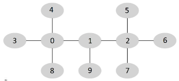
(a)

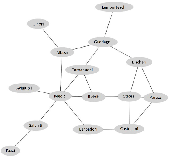
(b)

Figure 6: Graphs used to test the Self-consistency and Bridge axioms.
(a) Caterpillar $G_{14}$. (b) The Renaissance Florentine families marriage network $G_{15}$ [66].

TABLE II: Verification of the Self-consistency and Bridge axioms for the measures in ${{\cal F}^{40}}$. ‘$\bm{+}$’ indicates that the measure satisfies the axiom; ‘$\bm{+/-}$’ that it is satisfied by a slightly modified measure; ‘$\bm{-}$’ that the axiom is violated. In the latter case, a graph and an ordered pair of nodes are indicated for which the axiom is violated. “Comm.” is short for Communicability.

Centrality measures	Self-consistency	Bridge axiom
1. Betweenness	$-_{(0,3)G_{4}}$	$-_{(0,5)G^{\prime}_{5}}$
2. Closeness	$-_{(0,3)G_{4}}$	$+$
3. Connectivity	$-_{(0,3)G_{4}}$	$+$
4. Connectedness power	$-_{(0,3)G_{4}}$	$-_{(0,5)G_{5}}$
5. Degree	$-_{(0,4)G_{2}}$	$-_{(0,5)G_{5}}$
6. Coreness	$-_{(0,1)G_{7}}$	$-_{(0,5)G_{5}}$
7. Bridging	$-_{(0,3)G_{4}}$	$-_{(0,5)G_{5}}$
8. PageRank	$-_{(0,3)G_{4}}$	$-_{(0,5)G_{5}}$
9. Harmonic closeness	$-_{(0,3)G_{4}}$	$-_{(0,5)G_{5}}$
10. Eccentricity	$-_{(0,4)G_{2}}$	$-_{(0,5)G_{5}}$
11. $p$-Means,  $p=-2$	$-_{(0,3)G_{4}}$	$-_{(0,5)G_{5}}$
12. $p$-Means,  $p=0$	$-_{(0,3)G_{4}}$	$-_{(0,5)G_{5}}$
13. $p$-Means,  $p=2$	$-_{(0,3)G_{4}}$	$-_{(0,5)G_{5}}$
14. Beta current flow	$-_{(0,3)G_{4}}$	$-_{(0,5)G_{5}}$
15. Weighted degree	$-_{(0,4)G_{2}}$	$-_{(1,2)G_{1}}$
16. Decaying degree	$-_{(1,5)G_{5}}$	$-_{(0,5)G_{5}}$
17. Decay	$-_{(0,3)G_{4}}$	$-_{(0,5)G_{5}}$
18. Generalized degree	$+$	$-_{(0,5)G_{5}}$
19. Katz	$+$	$-_{(0,5)G_{5}}$
20. Eigenvector	$+$	$-_{(0,5)G_{5}}$
21. Bonacich	$+$	$-_{(0,5)G_{5}}$
22. Total communicability	$-_{(8,9)G_{14}}$	$-_{(0,5)G_{5}}$
23. Communicability$(K_{ij})$	$-_{(8,9)G_{14}}$	$-_{(0,5)G_{5}}$
24. Walk$(K_{ij})$	$-_{(8,9)G_{14}}$	$-_{(0,5)G_{5}}$
25. Walk$(K_{ii})$	$-_{\mbox{\scriptsize(Bischeri,Peruzzi)}G_{15}}$	$-_{(0,5)G_{5}}$
26. Estrada	$-_{\mbox{\scriptsize(Bischeri,Peruzzi)}G_{15}}$	$-_{(0,5)G_{5}}$
27. Eigencentrality(Dice)	$-_{(3,6)G_{9}}$	$-_{(0,5)G_{5}}$
28. Eigencentrality(Jaccard)	$-_{(3,6)G_{9}}$	$-_{(0,5)G_{5}}$
29. Closeness(Forest)	$-_{(1,5)G_{5}}$	$-_{(0,5)G_{5}}$
30. Closeness(Heat)	$-_{(1,5)G_{5}}$	$-_{(0,5)G_{5}}$
31. Closeness(logForest)	$-_{(0,3)G_{4}}$	$\!\!\!+/-_{(0,5)G_{5}}$
32. Closeness(logWalk)	$-_{(0,3)G_{4}}$	$\!\!\!+/-_{(0,5)G_{5}}$
33. Closeness(logHeat)	$-_{(0,3)G_{4}}$	$-_{(0,5)G_{5}}$
34. Closeness(logComm.)	$-_{(0,3)G_{4}}$	$-_{(0,5)G_{5}}$
35. Eccentricity(Forest)	$-_{(0,1)G_{7}}$	$-_{(0,5)G_{5}}$
36. Eccentricity(Heat)	$-_{(0,1)G_{7}}$	$-_{(0,5)G_{5}}$
37. Eccentricity(logForest)	$-_{(0,1)G_{7}}$	$-_{(0,5)G_{5}}$
38. Eccentricity(logWalk)	$-_{(0,1)G_{7}}$	$-_{(0,5)G_{5}}$
39. Eccentricity(logHeat)	$-_{(0,1)G_{7}}$	$-_{(0,5)G_{5}}$
40. Eccentricity(logComm.)​​	$-_{(0,1)G_{7}}$	$-_{(0,5)G_{5_{\mathstrut}}}$

Table II presents the results of verification of the Self-consistency and Bridge axioms for the centralities in ${{\cal F}^{40}}$. It turns out that only four measures satisfy Self-consistency. Four other measures satisfy the Bridge axiom, including two measures that do so after a slight modification. When a measure violates an axiom, a record of the form ‘$-_{(u,v)G_{k}}\!$’ indicates that the axiom is violated, in particular, for the ordered pair of nodes $(u,v)$ in graph $G_{k}.$ Graphs $G_{1}$ to $G_{13}$ are shown in Fig. 1; two additional graphs found in Table II, $G_{14}$ and $G_{15},$ are shown in Fig. 6. Graph $G^{\prime}_{5}$ is obtained from $G_{5}$ by replacing $E(G_{5})$ with $E(G_{5})\smallsetminus\{\{1,2\}\}.$

The following propositions describe the positive results in Table II.

Proposition 1 ([41]).

The Generalized degree, Eigenvector, Katz, and Bonacich centralities satisfy Self-consistency.

The second result includes Closeness${}^{*}(\log$Forest$)$ and Closeness${}^{*}(\log$Walk$)$ introduced in Materials and Methods. They are based on cutpoint additive distances as distinct from Closeness$(\log$Forest$)$ and Closeness$(\log$Walk$)$ included in ${{\cal F}^{40}}$. This property enforces the Bridge axiom.

Proposition 2 ([41]).

The Closeness, Closeness${}^{*}(\log$Forest$)$, Closeness${}^{*}(\log$Walk$)$, and Connectivity centralities satisfy the Bridge axiom.

It follows from Lemma 1 in [41] that other strictly positive transitional measures [67] and cutpoint additive distances also produce centralities that satisfy the Bridge axiom.

Suppose the expert believes that all appropriate centralities must satisfy Self-consistency (or Bridge axiom). This leads to a drastic reduction of the set ${{\cal F}^{40}}$ and the culling survey.

The decision trees for the subsets of centralities satisfying the Self-Consistency or Bridge axiom are shown in Fig. 7 and Fig. 8, respectively.

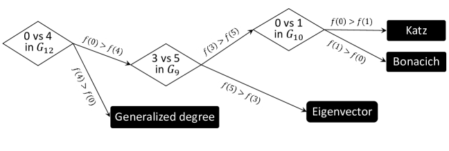
Figure 7: A decision tree for the measures in ${{\cal F}^{40}}$ satisfying Self-consistency.

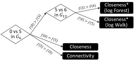
Figure 8: A decision tree for the four measures satisfying the Bridge axiom.

The first one can be extracted from the general tree of Figures 3 and 4. The second tree involves graphs that separate Closeness${}^{*}(\log$Forest$)$ and Closeness${}^{*}(\log$Walk$)$ from each other and the other measures that satisfy the Bridge axiom.

Some of the questions in the survey of Fig. 7 may not be easy to answer. This is due to the fact that the measures satisfying Self-consistency, as Lemma 2 in [41] shows, have the same operating principle based on supporting neighborhood representations, so the difference between them can be quite subtle. The comparison “0 vs 1 in $G_{10}$” can be replaced by “2 vs 6 in $G_{11}$” with $f(6)>f(2)$ leading to Katz centrality and $f(2)>f(6)$ yielding Bonacich centrality (which is a variation of Katz centrality) with the parameter values specified in Materials and Methods.

III Discussion

In this paper, we proposed a method called culling for selecting a point centrality measure based on expert understanding of how a measure suitable for a particular application should act on test graphs. The method consists of the following steps:

• Choosing a finite set ${\cal F}$ of candidate measures, among which there are no rank equivalent measures;

• Generating a list of small (if possible) test graphs that separate all measures in ${\cal F}$;

• Compiling a decision-tree survey composed of questions about the comparative centrality of test nodes in the test graphs;

• Completing the survey to obtain a centrality measure consistent with the expert’s responses.

The developed procedures enable one to apply the culling method to any finite set ${\cal F}$ of centrality measures.

The conclusions are as follows.

1. Centrality measures based on rational ideas and satisfying reasonable axioms may behave counterintuitively (in the logic of a particular application or even in general) on small test graphs. This was seen in the examples of Weighted degree, PageRank, dissimilarity based Eigencentralities, and some other measures. Therefore, examining the performance of measures on test graphs is a good complement to typological, axiomatic, and data-driven methods of analysis. Poor results of such tests indicate inherent weaknesses in the measures and leave little chance for high-quality processing of real data.

2. The culling method relies on the expert’s ability to judge with some certainty which of two nodes in a fairly simple graph has a higher centrality. We assume that this ability can be based upon both the findings of prior studies and cumulative experience. Moreover, the certainty of such a judgment is often stronger than the appeal of the heuristics behind a measure. Given a set of centralities, the culling method generates a decision-tree survey for selecting the measure that best fits the expert concept of centrality. The implementation of the method varies depending on the choice of graphs for separating measures. In this paper, we studied a test set ${{\cal F}^{40}}$ consisting of forty centralities, which included, among others, several kernel-based closeness, eccentricity and other measures introduced in Materials and Methods. It contained many couples of closely related measures, and we were interested in whether large or dense graphs are necessary to separate them. The answer is no: we opted for $1$-trees (unicycles), and 13 graphs of this class of order $8$ (just one graph) or lower with node degrees at most $4$ were sufficient to separate all the measures in ${{\cal F}^{40}}$. For the case of an arbitrary set of measures, a general procedure was proposed.

3. If a set of measures ${\cal F}$ is updated to a new set ${\cal F}^{\prime}\supset{\cal F},$ then the culling method adapts by extending the existing decision tree to accommodate the changes.

4. The culling method generates a collection of triples in the form of a graph and a pair of its nodes that distinguish each measure in the set ${\cal F}$ from others. The centrality inequalities/equalities on these triples form the “profile” of a measure characterizing its behavior and helping to decide whether to accept or discard it. They can also be used to classify measures. In this way, culling allows one to reveal some perplexing features of centralities. Examples have been mentioned in Item 1 of the conclusions. As another example consider the Bridging centrality [50]. The expert who chooses it must approve the following claims of this measure (see Fig. 1): $f(0)>f(2)$ in $G_{2};$ $f(3)>f(4)$ in $G_{4};$ $f(5)>f(3)$ in $G_{6}$ and $G_{7};\,$ $f(5)>f(0)>f(1)$ in $G_{8};$ $f(4)>f(2)$ in $G_{9};$ $f(5)>f(1)$ in $G_{11},$ and $f(0)=f(1)$ in $G_{1}.$

5. A decision tree for the entire set of known centralities can be built by extending the tree presented above (Figures 3 and 4). Such a dendrogram may be useful (along with correlation-based methods [3]) for hierarchical clustering of measures. This is suggested by the fact that the tree for ${{\cal F}^{40}}$ contains several subtrees whose leaves correspond to closely related centralities. For example, Callout B (Fig. 4) consists of Eccentricity measures; Callout C comprises Closeness measures and the related Decaying degree; three measures satisfying Self-consistency belong to Callout D, while the fourth one is a “sister” of it. The reason for this is that the survey begins with the simplest graphs, while subtle differences between kindred measures are distinguished by more complex graphs that appear later in the survey.

6. On the other hand, relying solely on culling for selecting a single output measure from an extensive set of input measures may not be entirely robust. Indeed, the corresponding survey may contain rather difficult questions, the answers to which may not be confident enough, which can lead to an unstable result. To enhance reliability, option “not sure” can be added to the survey forms, potentially leading to multiple outcome. The choice among the resulting measures can be made by analyzing their application to real networks and checking their adherence to credible axioms. Moreover, the expert may take the survey multiple times to obtain a comprehensive picture by using relevant centralities of several types (cf. [12, 21]).

7. A promising application of the culling method is to combine it with a normative approach by constructing decision trees for subsets of measures that satisfy the most credible axioms. The paper presents short surveys for the measures in ${{\cal F}^{40}}$ (or their slight modifications) that meet the Self-consistency or Bridge axioms.

Thus, the recommended approach to address the question posed in the paper’s title is to utilize a strategy that encompasses several elements: verification of compliance with the most important axioms, culling, consideration of computational complexity factors, experimental studies involving statistical methods and machine learning, as well as a typological perspective that connects network dynamics to the underlying assumptions and concepts of each centrality measure.

Among these components, the culling method stands out as one of the least labor-intensive and time-consuming. It relies on expert knowledge while its procedures are transparent.

This study identifies several directions for future research. Here are some of those topics:

• Explore larger culling surveys;

• Collect and analyze statistics of survey results from diverse experts to obtain a measure attractiveness rating;

• Construct decision trees for subsets of measures that satisfy crucial axioms, such as monotonicity conditions, and their combinations;

• Adapt the culling method to centrality measures designed for directed networks;

• Utilize decision tree theory [68] to develop variations of the proposed procedure for constructing culling trees;

• Enhance the flexibility of culling surveys by (a) allowing the “not sure” option, (b) employing all graphs in ${\cal G}$ that separate specific pairs of measures, (c) allowing experts to utilize their own test graphs to select measures, (d) enabling experts to report confidence levels in their answers;

• Create an interactive web application implementing culling surveys for any chosen subset of centrality measures;

• Apply the culling approach to the problem of selecting scoring methods for unbalanced tournaments [63].

IV Materials and Methods

IV-A Closeness and Eccentricity Centralities Induced by Graph Kernels

In this section, we present several new classes of centrality measures used in Test Survey and subsequent sections. More information about them can be found in [69, 41].

Let $d(u,v)$ be the shortest path distance between nodes $u$ and $v$ of a graph $G$, i.e., the length of a shortest path between $u$ and $v.$ Two popular distance based centrality measures are the [shortest path] Closeness [44]

$$f(u)=\Big{(}\sum_{v\in V}d(u,v)\Big{)}^{-1},\quad u\in V$$ (2)

and [shortest path] Eccentricity [44]

$$f(u)=(\max_{v\in V}d(u,v))^{-1},\quad u\in V.$$ (3)

General classes of Closeness and Eccentricity centralities are defined by (2) and (3) with $d(u,v)$ being arbitrary distances for graph nodes. In the literature, several classes of such distances and, more generally, dissimilarity measures have been proposed (see, e.g., [70, 71, 69]). Many of them are defined via graph kernels. Let us consider four classes of them.

1. The parametric Katz [48] kernels (also referred to as Walk [72] or Neumann diffusion [71] kernels) are defined as

$$P^{{\operatorname{Walk}}}(t)=\sum_{k=0}^{\infty}(tA)^{k}=(I-tA)^{-1}$$ (4)

with $0<t<(\rho(A))^{-1},$ where $A=(a_{ij})$ is the adjacency matrix of $G$ and $\rho(A)$ is the spectral radius of $A.$

2. The Communicability kernels [47] are

$$P^{\operatorname{Comm}}(t)=\sum_{k=0}^{\infty}\frac{(tA)^{k}}{k!}=\exp(tA),\quad t>0.$$

Two other classes are defined similarly via the Laplacian matrix

$$L=\mathop{\mathrm{diag}}(A\bm{1})-A,$$

where $\bm{1}=(1,\ldots,1)^{T}$ and $\mathop{\mathrm{diag}}(\bm{x})$ is the diagonal matrix with vector $\bm{x}$ on the diagonal.

3. The Forest kernels, or regularized Laplacian kernels [73] are

$$P^{\operatorname{For}}(t)=(I+tL)^{-1},\;\;\mbox{where}\;\;t>0.$$ (5)

4. The Heat kernels are the Laplacian exponential diffusion kernels [54]

$$P^{\operatorname{Heat}}(t)=\sum_{k=0}^{\infty}\frac{(-tL)^{k}}{k!}=\exp(-tL),\quad t>0.$$

By Schoenberg’s theorem [74], if matrix $P=(p_{uv})$ is a kernel (i.e., is positive semidefinite), then it produces a Euclidean distance $d(u,v)$ by means of the transformation

$$d(u,v)=\big{(}\tfrac{1}{2}(p_{uu}+p_{vv}-p_{uv}-p_{vu})\big{)}^{\frac{1}{2}},\quad u,v\in V,$$ (6)

where $\frac{1}{2}$ is the scaling factor.

Thus, all Walk, Communicability, Forest, and Heat kernels with appropriate parameter values provide distances of the form (6) whose substitution in (2) and (3) yields Closeness and Eccentricity centralities. We will denote them by Closeness(Kernel) and Eccentricity(Kernel) with the corresponding kernels substituted.

Furthermore, if $P_{n\times n}=(p_{uv})$ determines a proximity measure (which means that for any $x,y,z\in V,$  $p_{xy}+p_{xz}-p_{yz}\leq p_{xx}$, and the inequality is strict whenever $z=y$ and $y\neq x$), then [75] transformation

$$d(u,v)=\tfrac{1}{2}(p_{uu}+p_{vv}-p_{uv}-p_{vu}),\quad u,v\in V$$ (7)

provides a distance function that satisfies the axioms of a metric. The Forest kernel with any $t>0$ produces a proximity measure, while kernels in the remaining three classes do so when $t$ is sufficiently small [69]. The centralities obtained from a Proximity measure by transformation (7) and substitution of the resulting distance into (2) and (3) are denoted in the present paper by Closeness${}^{*}($Proximity$)$ and Eccentricity${}^{*}($Proximity$)$, respectively.

Moreover, if $P$ represents a strictly positive transitional measure on $G$ (i.e., $p_{xy}\,p_{yz}\leq p_{xz}\,p_{yy}$ for all nodes $x,y,$ and $z,$ with $p_{xy}\,p_{yz}=p_{xz}\,p_{yy}$ whenever every path in $G$ from $x$ to $z$ visits $y$), then transformation

$$\hat{p}_{uv}=\ln p_{uv},\quad u,v\in V$$ (8)

produces [67, 70] a proximity measure. In this case, (7) applied to $\hat{P}=(\hat{p}_{uv})$ reduces to

$$d(u,v)=\tfrac{1}{2}(\ln p_{uu}+\ln p_{vv}-\ln p_{uv}-\ln p_{vu})$$ (9)

and generates [70] a cutpoint additive distance $d(u,v),$ viz., such a distance that $d(u,v)+d(v,w)=d(u,w)$ whenever $v$ is a cutpoint between $u$ and $w$ in $G$ (or, equivalently, whenever all paths connecting $u$ and $w$ visit $v$). The centralities obtained from any ​Transitional_Measure by transformation (9) and substitution of the resulting distance into (2) and (3) are denoted by Closeness${}^{*}($$\log$Transitional_Measure$)$ and Eccentricity${}^{*}($$\log$Transitional_Measure$)$, respectively.

Since the Walk and Forest kernels determine [67] strictly positive transitional measures, transformation (9) applied to them generates cutpoint additive distances. Substituting them into (2) and (3) produces Closeness${}^{*}(\log$Forest$)$ and Closeness${}^{*}(\log$Walk$)$, as well as the corresponding Eccentricity${}^{*}(\cdot)$ measures.

Thus, based on the above properties, we define Closeness and Eccentricity centralities obtained by substituting the:

• Forest kernel;

• Heat kernel;

• logarithmic Forest kernel;

• logarithmic Walk kernel;

• logarithmic Heat kernel, and

• logarithmic Communicability kernel

transformed by (6) or (7) into (2) and (3). These centralities are included in the test survey. We set $t=1$ for the Forest, Heat, and Communicability kernels and $t=(\rho(A)+1)^{-1}$ for the Walk kernel. Regarding other measures, we use PageRank centrality with $\alpha=0.85$, Generalized degree with $\varepsilon=2$, Decay centrality with $\delta=0.9$, Katz centrality with $a=(\rho(A)+1)^{-1}$, and Bonacich centrality (which is a variation of Katz centrality) with $\alpha=1$ and $\beta=(\rho(A)+0.5)^{-1}.$ The difference between the Katz and Bonacich centralities lies in the difference in their parameters $a$ and $\beta$.

The Closeness^∗(Forest) centrality was examined in [76] with the conclusion that “forest distance centrality has a better discriminating power than alternate metrics such as betweenness, harmonic centrality, eigenvector centrality, and PageRank.” The authors of [76] believe that the order of node importance induced by the forest distances on simple graphs is “consistent with human intuition.” The $t\to\infty$ case of this centrality is [53] the Resistance centrality featuring in [10].

IV-B Some Other Kernel-based Centralities

While the above measures are meaningful kernel-based centralities, they do not exhaust all kernels and transformations [71, 69] that can be used to obtain such measures. To mention some alternative constructions, note that each distance on graph nodes can be integrated in the harmonic closeness framework [52], $p$-Means framework [33], or the framework developed in [31].

Furthermore, kernels and similarity/proximity measures can be used to obtain centralities directly, without transformations into distances. An example of such measures is the Estrada subgraph centrality [47]. This index of a graph node $u$ is equal to the diagonal entry $p^{\operatorname{Comm}}_{uu}$ of the Communicability kernel, so we denote it by Communicability$(K_{ii}).$ Similarly, Walk$(K_{ii})$ is the measure $f(u)=p^{{\operatorname{Walk}}}_{uu},$ $u\in V$ determined by the diagonal entries of the Walk kernel.

One more type of centrality measures is constructed by summing the non-diagonal entries of the rows of a kernel matrix. We consider the measures of this kind Communicability($K_{ij}$) and Walk($K_{ij})$ defined by $f(u)=\sum_{v\neq u}p^{\operatorname{Comm}}_{uv}$ and $f(u)=\sum_{v\neq u}p^{{\operatorname{Walk}}}_{uv},$ $u\in V,$ respectively. Finally, Total communicability [45] is obtained by summing all row entries of the Communicability kernel: $f(u)=\sum_{v\in V}p^{\operatorname{Comm}}_{uv}$; it can be described [77] in terms of “potential gain.” The Total walk measure $f(u)=\sum_{v\in V_{\mathstrut}}p^{\operatorname{Walk}}_{uv}=(P^{\operatorname{Walk}}\hskip 0.70007pt\bm{1})_{u}$ is order equivalent to the Katz centrality [48] expressed as $f(u)=((P^{\operatorname{Walk}}-I)\bm{1})_{u}$.

Note that the existence of hundreds of types and subtypes of centrality, coupled by the existence of infinite families of measures, highlights the need for powerful tools for comparing centrality indices and selecting the most appropriate ones.

References

- [1] “Centiserver: The most comprehensive centrality resource and web application for centrality measures calculation,” [Online]. Available: https://www.centiserver.org/?q1=centrality, 2023.
- [2] L. Lü, D. Chen, X.-L. Ren, Q.-M. Zhang, Y.-C. Zhang, and T. Zhou, “Vital nodes identification in complex networks,” Phys. Reports, vol. 650, pp. 1–63, 2016.
- [3] A. Saxena and S. Iyengar, “Centrality measures in complex networks: A survey.” arXiv, pp. 1–75, 2020, https://arxiv.org/abs/2011.07190.
- [4] Z. Wan, Y. Mahajan, B. W. Kang, T. J. Moore, and J.-H. Cho, “A survey on centrality metrics and their network resilience analysis,” IEEE Access, vol. 9, pp. 104 773–104 819, 2021.
- [5] N. E. Friedkin, “Theoretical foundations for centrality measures,” Am. J. Sociol., vol. 96, no. 6, pp. 1478–1504, 1991.
- [6] S. P. Borgatti, “Centrality and network flow,” Soc. Networks, vol. 27, no. 1, pp. 55–71, 2005.
- [7] Z. Wang, A. Scaglione, and R. J. Thomas, “Electrical centrality measures for electric power grid vulnerability analysis,” in 49th IEEE Conference on Decision and Control CDC. IEEE, 2010, pp. 5792–5797.
- [8] A. G. Chkhartishvili, D. A. Gubanov, and D. A. Novikov, Social Networks: Models of Information Influence, Control and Confrontation. Springer, 2019.
- [9] D. A. Gubanov and A. G. Chkhartishvili, “Influence levels of users and meta-users of a social network,” Autom. Remote Control, vol. 79, no. 3, pp. 545–553, 2018.
- [10] M. Tyloo, L. Pagnier, and P. Jacquod, “The key player problem in complex oscillator networks and electric power grids: Resistance centralities identify local vulnerabilities,” Science Advances, vol. 5, no. 11, p. eaaw8359, 2019.
- [11] A. Saxena, “A survey of evolving models for weighted complex networks based on their dynamics and evolution.” arXiv, pp. 1–43, 2020, https://arxiv.org/abs/2012.08166.
- [12] K. Vignery and W. Laurier, “A methodology and theoretical taxonomy for centrality measures: What are the best centrality indicators for student networks?” PLoS One, vol. 15, no. 12, p. e0244377, 2020.
- [13] R. Yousefi Nooraie, J. E. Sale, A. Marin, and L. E. Ross, “Social network analysis: An example of fusion between quantitative and qualitative methods,” J. Mix. Methods Res., vol. 14, no. 1, pp. 110–124, 2020.
- [14] F. Bloch, M. O. Jackson, and P. Tebaldi, “Centrality measures in networks,” Soc. Choice Welf., vol. 61, pp. 413–453, 2023.
- [15] J. M. Bolland, “Sorting out centrality: An analysis of the performance of four centrality models in real and simulated networks,” Soc. Networks, vol. 10, no. 3, pp. 233–253, 1988.
- [16] R. B. Rothenberg, J. J. Potterat, D. E. Woodhouse, W. W. Darrow, S. Q. Muth, and A. S. Klovdahl, “Choosing a centrality measure: Epidemiologic correlates in the Colorado Springs study of social networks,” Soc. Networks, vol. 17, no. 3-4, pp. 273–297, 1995.
- [17] K. Batool and M. A. Niazi, “Towards a methodology for validation of centrality measures in complex networks,” PLoS One, vol. 9, no. 4, p. e98379, 2014.
- [18] J. Cao, Z. Bu, Y. Wang, H. Yang, J. Jiang, and H.-J. Li, “Detecting prosumer-community groups in smart grids from the multiagent perspective,” IEEE Trans. Syst., Man, Cybern., Syst., vol. 49, no. 8, pp. 1652–1664, 2019.
- [19] S. Oldham, B. Fulcher, L. Parkes, A. Arnatkevičiūtė, C. Suo, and A. Fornito, “Consistency and differences between centrality measures across distinct classes of networks,” PLoS One, vol. 14, no. 7, p. e0220061, 2019.
- [20] H. Rastogi and M. Jain, “A correlative study of centrality measures across real-world networks,” in 2020 Fourth International Conference on I-SMAC. IEEE, 2020, pp. 987–994.
- [21] G. Brysbaert and M. F. Lensink, “Centrality measures in residue interaction networks to highlight amino acids in protein–protein binding,” Front. Bioinforma., vol. 1, p. 684970, 2021.
- [22] D. F. Sakellariou, A. Vakrinou, M. Koutroumanidis, and M. P. Richardson, “Neurocraft: Software for microscale brain network dynamics,” Sci. Reports, vol. 11, no. 1, p. 20716, 2021.
- [23] M. Ashtiani, A. Salehzadeh-Yazdi, Z. Razaghi-Moghadam, H. Hennig, O. Wolkenhauer, M. Mirzaie, and M. Jafari, “A systematic survey of centrality measures for protein-protein interaction networks,” BMC Syst. Biol., vol. 12, no. 1, pp. 1–17, 2018, article number: 80.
- [24] R. Holzman, “An axiomatic approach to location on networks,” Math. Oper. Res., vol. 15, no. 3, pp. 553–563, 1990.
- [25] R. Vohra, “An axiomatic characterization of some locations in trees,” Eur. J. Oper. Res., vol. 90, no. 1, pp. 78–84, 1996.
- [26] H. Monsuur and T. Storcken, “Centers in connected undirected graphs: An axiomatic approach,” Oper. Res., vol. 52, no. 1, pp. 54–64, 2004.
- [27] M. Garg, “Axiomatic foundations of centrality in networks,” Mimeo, Stanford University, Tech. Rep., 2009, [Online]. Available: https://papers.ssrn.com/sol3/papers.cfm?abstract_id=1372441.
- [28] V. Dequiedt and Y. Zenou, “Local and consistent centrality measures in parameterized networks,” Math. Soc. Sci., vol. 88, pp. 28–36, 2017.
- [29] O. Skibski and J. Sosnowska, “Axioms for distance-based centralities,” in Thirty-Second AAAI Conference on Artificial Intelligence AAAI–18, 2018, pp. 1218–1225.
- [30] T. Wąs and O. Skibski, “Axiomatic characterization of PageRank,” Artif. Intell., vol. 318, p. 103900, 2023.
- [31] F. Agneessens, S. P. Borgatti, and M. G. Everett, “Geodesic based centrality: Unifying the local and the global,” Soc. Networks, vol. 49, pp. 12–26, 2017.
- [32] L. Csató, “Measuring centrality by a generalization of degree,” Cent. Eur. J. Oper. Res., vol. 25, no. 4, pp. 771–790, 2017.
- [33] R. L. de Andrade and L. C. Rêgo, “-means centrality,” Commun. Nonlinear Sci. Numer. Simul., vol. 68, pp. 41–55, 2019.
- [34] M. L. Mágó, “Power values and framing in game theory,” Ph.D. dissertation, CentER, Tilburg University, 2018.
- [35] S. Bandyopadhyay, M. N. Murty, and R. Narayanam, “A generic axiomatic characterization of centrality measures in social network.” arXiv, pp. 1–20, 2017, https://arxiv.org/abs/1703.07580.
- [36] S. Brin and L. Page, “The anatomy of a large-scale hypertextual web search engine,” Comput. Networks ISDN Syst., vol. 30, no. 1–7, pp. 107–117, 1998.
- [37] A. N. Langville and C. D. Meyer, Google’s PageRank and Beyond: The Science of Search Engine Rankings. Princeton University Press, 2006.
- [38] K. Avrachenkov and M. Dreveton, Statistical Analysis of Networks. Boston–Delft: Now Publishers, 2022.
- [39] N. E. Friedkin and E. C. Johnsen, “Two steps to obfuscation,” Soc. Networks, vol. 39, pp. 12–13, 2014.
- [40] A. Altman and M. Tennenholtz, “Ranking systems: The PageRank axioms,” in Proceedings of the 6th ACM Conference on Electronic Commerce. ACM, 2005, pp. 1–8.
- [41] P. Chebotarev, “Selection of centrality measures using self-consistency and bridge axioms.” arXiv, pp. 1–21, 2023, https://arxiv.org/abs/2301.00084, accepted for publication in J. Complex Networks.
- [42] L. C. Freeman, “A set of measures of centrality based on betweenness,” Sociometry, vol. 40, no. 1, pp. 35–41, 1977.
- [43] P. Bonacich, “Power and centrality: A family of measures,” Am. J. Sociol., vol. 92, no. 5, pp. 1170–1182, 1987.
- [44] A. Bavelas, “A mathematical model for group structures,” Appl. Anthropol., vol. 7, no. 3, pp. 16–30, 1948.
- [45] M. Benzi and C. Klymko, “Total communicability as a centrality measure,” J. Complex Networks, vol. 1, no. 2, pp. 124–149, 2013.
- [46] A. Khmelnitskaya, G. van der Laan, and D. Talman, “The number of ways to construct a connected graph: A graph-based generalization of the binomial coefficients,” J. Integer Seq., vol. 26, no. 23.4.3, 2023.
- [47] E. Estrada and J. A. Rodriguez-Velazquez, “Subgraph centrality in complex networks,” Phys. Rev. E, vol. 71, no. 5, p. 056103, 2005.
- [48] L. Katz, “A new status index derived from sociometric analysis,” Psychometrika, vol. 18, no. 1, pp. 39–43, 1953.
- [49] J. Bae and S. Kim, “Identifying and ranking influential spreaders in complex networks by neighborhood coreness,” Phys. A: Stat. Mech. Its Appl., vol. 395, pp. 549–559, 2014.
- [50] R. Breitling, P. Armengaud, A. Amtmann, and P. Herzyk, “Rank products: A simple, yet powerful, new method to detect differentially regulated genes in replicated microarray experiments,” FEBS Lett., vol. 573, no. 1–3, pp. 83–92, 2004.
- [51] A. Alvarez-Socorro, G. Herrera-Almarza, and L. González-Díaz, “Eigencentrality based on dissimilarity measures reveals central nodes in complex networks,” Sci. Reports, vol. 5, p. 17095, 2015.
- [52] M. Marchiori and V. Latora, “Harmony in the small-world,” Phys. A: Stat. Mech. its Appl., vol. 285, no. 3-4, pp. 539–546, 2000.
- [53] P. Chebotarev and E. Shamis, “The forest metrics for graph vertices,” Electron. Notes Discret. Math., vol. 11, pp. 98–107, 2002.
- [54] R. I. Kondor and J. Lafferty, “Diffusion kernels on graphs and other discrete structures,” in Proceedings of the 19th International Conference on Machine Learning, 2002, pp. 315–322.
- [55] P. Chebotarev, “A class of graph-geodetic distances generalizing the shortest-path and the resistance distances,” Discret. Appl. Math., vol. 159, no. 5, pp. 295–302, 2011.
- [56] ——, “The walk distances in graphs,” Discret. Appl. Math., vol. 160, no. 10–11, pp. 1484–1500, 2012.
- [57] K. E. Avrachenkov, V. V. Mazalov, and B. T. Tsynguev, “Beta current flow centrality for weighted networks,” in 4th International Conference on Computational Social Networks. Springer, 2015, pp. 216–227.
- [58] V. Ivashkin and P. Chebotarev, “Do logarithmic proximity measures outperform plain ones in graph clustering?” in Models, Algorithms, and Technologies for Network Analysis. Springer, 2016, pp. 87–105.
- [59] N. Tsakas, “On decay centrality,” The B. E. J. Theor. Econ., vol. 19, no. 1, pp. 1–18, 2018.
- [60] E. Landau, “Zur relativen Wertbemessung der Turnierresultate,” Deutsches Wochenschach, vol. 11, pp. 366–369, 1895.
- [61] “Choosing the most appropriate centrality measure: A sample interactive internet survey,” [Online]. Available: https://docs.google.com/forms/d/e/1FAIpQLSfeyetuPJV0wYDuRXxheHHyRaclfTVvfSRRz3oyesPcYUT6Dg/viewform, 2023.
- [62] P. Boldi, F. Furia, and S. Vigna, “Monotonicity in undirected networks.” arXiv, 2022, https://arxiv.org/abs/2207.06218.
- [63] P. Y. Chebotarev and E. Shamis, “Constructing an objective function for aggregating incomplete preferences,” in Econometric Decision Models. Berlin: Springer, 1997, pp. 100–124.
- [64] S. Bandyopadhyay, R. Narayanam, and M. N. Murty, “A generic axiomatic characterization for measuring influence in social networks,” in 24th International Conference on Pattern Recognition ICPR–2018. IEEE, 2018, pp. 2606–2611.
- [65] P. Chebotarev and E. Shamis, “Characterizations of scoring methods for preference aggregation,” Annals Oper. Res., vol. 80, pp. 299–332, 1998.
- [66] J. F. Padgett and C. K. Ansell, “Robust action and the rise of the Medici, 1400–1434,” Am. J. Sociol., vol. 98, no. 6, pp. 1259–1319, 1993.
- [67] P. Chebotarev, “The graph bottleneck identity,” Adv. Appl. Math., vol. 47, no. 3, pp. 403–413, 2011.
- [68] L. Rokach and O. Maimon, Data Mining with Decision Trees: Theory and Applications, 2nd ed. World Scientific, 2015.
- [69] K. Avrachenkov, P. Chebotarev, and D. Rubanov, “Similarities on graphs: Kernels versus proximity measures,” Eur. J. Comb., vol. 80, pp. 47–56, 2019.
- [70] P. Chebotarev, “Studying new classes of graph metrics,” in Proceedings of the SEE Conference “Geometric Science of Information” GSI–2013, ser. LNCS 8085. Berlin: Springer, 2013, pp. 207–214.
- [71] F. Fouss, M. Saerens, and M. Shimbo, Algorithms and Models for Network Data and Link Analysis. Cambridge University Press, 2016.
- [72] P. Y. Chebotarev and E. V. Shamis, “On proximity measures for graph vertices,” Autom. Remote Control, vol. 59, no. 10, pp. 1443–1459, 1998.
- [73] P. Y. Chebotarev and E. Shamis, “On the proximity measure for graph vertices provided by the inverse Laplacian characteristic matrix,” in Abstracts of the Conference “Linear Algebra and its Applications”. University of Manchester, 1995, pp. 6–7, Available: http://web.archive.org/web/20230314224253/http://www.ma.man.ac.uk/~higham/laa95/abstracts.ps.
- [74] I. J. Schoenberg, “Remarks to M. Fréchet’s article “Sur la définition axiomatique d’une classe d’espaces vectoriels distanciés applicables vectoriellement sur l’espace de Hilbert”,” Annals Math., vol. 36, pp. 724–732, 1935.
- [75] P. Y. Chebotarev and E. V. Shamis, “On a duality between metrics and -proximities,” Autom. Remote Control, vol. 59, pp. 608–612, 1998.
- [76] Y. Jin, Q. Bao, and Z. Zhang, “Forest distance closeness centrality in disconnected graphs,” in 2019 IEEE International Conference on Data Mining ICDM. IEEE, 2019, pp. 339–348.
- [77] P. De Meo, M. Levene, F. Messina, and A. Provetti, “A general centrality framework based on node navigability,” IEEE Trans. Knowl. Data Eng., vol. 32, no. 11, pp. 2088–2100, 2020.