Blending and obscuration in weak lensing magnification

Abstract

We test the impact of some systematic errors in weak lensing magnification measurements with the COSMOS 30-band photo-$z$ Survey flux limited to $I_{auto}<25.0$ using correlations of both source galaxy counts and magnitudes. Systematic obscuration effects are measured by comparing counts and magnification correlations. We use the ACS-HST catalogs to identify potential blending objects (close pairs) and perform the magnification analyses with and without blended objects. We find that blending effects start to be important ($\sim$ 0.04 mag obscuration) at angular scales smaller than 0.1 arcmin. Extinction and other systematic obscuration effects can be as large as 0.10 mag (U-band) but are typically smaller than 0.02 mag depending on the band. After applying these corrections, we measure a $3.9\sigma$ magnification signal that is consistent for both counts and magnitudes. The corresponding projected mass profiles of galaxies at redshift $z\simeq 0.6$ ($M_{I}\simeq-21$) is $\Sigma=25\pm 6M_{\sun}h^{3}/pc^{2}$ at 0.1 Mpc/h, consistent with NFW type profile with $M_{200}\simeq 2\times 10^{12}M_{\sun}h/pc^{2}$. Tangential shear and flux-size magnification over the same lenses show similar mass profiles. We conclude that magnification from counts and fluxes using photometric redshifts has the potential to provide complementary weak lensing information in future wide field surveys once we carefully take into account systematic effects, such as obscuration and blending.

1 Introduction

Gravitational lensing can be used to measure the total matter distribution projected onto the sky (for a review see Bartelmann & Schneider 2001) and in combination with galaxy clustering provides a powerful tool to study cosmology and structure formation (see e.g. Bernstein & Cai 2011, Cai & Bernstein 2012, Gaztanaga et al. 2012, Weinberg et al. 2013, Eriksen & Gaztanaga 2015a-c, Eriksen & Gaztanaga 2018).

In the weak lensing regime gravitational distortions result in shear and magnification in the shapes, sizes, fluxes, and counts of galaxies in the background of the lenses we want to study. Magnification changes the observed galaxy fluxes and this manifests itself in two separate observational quantities: galaxy number counts (e.g. see Schneider 1987, Narayan 1989) and magnitude-counts cross-correlations (e.g. see Menard et al. 2010). In this paper we will focus on these two effects and will compare them to magnification from galaxy sizes and shear derived from shapes using the same galaxy sample (Schmidt et al. 2012). Van Waerbeke (2010) discusses the cosmological gain from combining magnification and shear.

The magnification signal from cross-correlation of galaxy samples is small (a per cent level change in clustering on arcminute scales) while the corresponding statistical noise (from the auto-correlation of the samples) can be large. We therefore need either a large area or large density to sample enough galaxy pairs to achieve a significant signal-to-noise ratio (SNR) magnification measurement. These two situations are complementary because the survey cost is proportional to the total number of objects and therefore the number of pairs available. The two common strategies are to use either low densities with large survey area or high densities with small survey area. The former samples large scales (mainly probing the 2-halo term) while the latter is usually restricted to small scales (probing the 1-halo term). Besides SNR we also need accuracy of the measurements and there are several systematic bias that can affect such small cross-correlation signal (see Hildebrandt et al. 2016).

Current magnification measurements have been achieved over dilute spectroscopic samples spread over large areas (e. g. Scranton et al. 2005, Bauer et al. 2014). Samples are well separated in redshifts by selecting foreground spectroscopic subsamples (e. g. LRG or clusters) which are cross-correlated with high redshift selected samples: spectroscopic QSO (e. g.  Gaztanaga 2003, Menard et al. 2010) or photometric Dropout Galaxies (e. g. Hildebrant et al. 2009, Morrison et al. 2012). These measurements therefore sample large (2-halo terms) correlations. The small scale weak lensing regime (of 1-halo term) is currently better explored with sheared shape measurements over smaller and denser samples using the Hubble Space Telescope (HST) Advanced Camera for Surveys (ACS) (e. g. Leuthaud et al. 2007 and references therein) or larger ground based WL Surveys such as Deep Lens Survey (Wittman et al. 2002, Jee et al. 2013), CFHTLenS (Heymans et al. 2013, Ford et al 2015), KIDS (Hildebrandt et al. 2017), DES (Abbott et al. 2018), or HSC (Hikage et al. 2019).

Schmidt et al. (2012) presented one of the few existing comparisons of magnification and shear measurements using the same lens samples. This work uses the same COSMOS reference catalog as the one we use in our analysis. The main difference with Schmidt et al. (2012) is that we use flux limited samples (rather than galaxy groups) for lenses, and that we estimate magnification from the combination of flux and (HST) sizes, while here we focus on magnification from counts and fluxes. The motivation for our approach is to test systematic effects in magnification measurements of deep samples where morphological (space based) information is not available or is not that reliable. We will also compare our results with those using shear and flux-size magnification for the same lens samples.

Future deep photometric surveys, such as the Legacy Survey of Space and Time (LSST) to be carried out in 2022-2032 by the the Rubin Observatory, Euclid, and WFIRST, have the potential to measure magnification for flux limited samples (e.g. the LSST Science Book). For deep samples ($I_{auto}>25$) ground based shape measurements are limited by systematics, and it might be harder to measure weak lensing from shapes and sizes than from flux and counts, as presented in this paper. But there are several systematic effects that could limit the potential of such magnification measurements. Among them are: 1) the accuracy of the photometric redshift selection and characterization (which could add intrinsic cross-correlation) 2) flux/count obscuration effects due to the atmosphere, extinction or data reduction (e.g background subtraction) 3) blending of sources, which can affect both the counts and the fluxes. In this paper we explore these three effects in a working example, the COSMOS field which has a wealth of deep and accurate data, including space based observations, to explore some of these issues.

This paper is organized as follows. In §2 we present the modelling of the magnification, obscuration and blending effects. In §3 we present the data selection and validation. In §4 we present the magnificaiton results to finish with the conclusions in §5.

2 Modeling

In this section we discuss how magnification can be measured using either galaxy counts or fluxes. We also present a method to combine cross-correlation measurements of density fluctuations (counts) and magnitudes (or fluxes) to account for systematic effects. §2.1 introduces the definition of magnification and shows its effects on individually observed magnitudes. §2.2 adds the impact of obscuration to observed magnitudes, while §2.3 shows how counts can be affected by magnification and obscuration. The effects of blending are presented in §2.4. §2.5 proposes a way to separate the effects of magnification and obscuration, while §2.6 introduces the cross-correlation measurements that we use in this paper.

2.1 Magnification

Magnification of flux $\mu$ in gravitational lensing distortion is:

$$\mu\equiv 1+\delta_{\mu}={1\over{detA}}={1\over{(1-\kappa)^{2}-|\gamma|^{2}}}$$ (1)

where $A$ is the Jacobian matrix for the lensing transformation (see e.g. Bartelmann & Schneider 2000). In the weak lensing (WL) regime, fluctuations in magnification $\delta_{\mu}$, convergence $\kappa$ and shear $\gamma$ are closely related. Small fluctuations in convergence $\delta_{\kappa}$, according to Eq.1, are half as large as magnification $\delta_{\mu}=2\delta_{\kappa}$.

The measured flux $F$ is changed relative to the emitted flux $F_{0}$ as $F=F_{0}\mu$. So the change to the apparent magnitude in band $\lambda$ is :

$$\delta m_{\lambda}=-{2.5\over{\ln{10}}}\delta_{\mu}$$ (2)

which is independent of the observational wavelength $\lambda$ used to measure the flux. This independence is helpful in separating the magnification signal from systematic effects that are chromatic, such as obscuration.

2.2 Magnitudes and Obscuration

In addition to magnification, observed magnitudes can be biased by galactic and extra galactic extinction/absorption, optical and atmospheric variations, blending and errors in the process of data imaging reduction (e.g. see for example Chang et al. 2015). From now on we will refer to the ensemble of all these effects as “obscuration" and we will not attempt to disentangle the different possible origins of these contributions. However, we will attempt to disentangle them from magnification by comparing their impact on magnitudes and counts.

The measured flux $F$ is changed as $F=F_{0}\mu e^{-\tau_{\lambda}}$ where $\tau_{\lambda}$ is the optical depth for obscuration effects and $F_{0}$ is the flux in the absence of obscuration. So the total combined change in observed magnitude due to magnification and obscuration is then:

$$\delta m_{\lambda}={2.5\over{\ln{10}}}\left(\tau_{\lambda}-\delta_{\mu}\right)=-{2.5\over{\ln{10}}}\delta_{\mu}+A_{\lambda}$$ (3)

where $A_{\lambda}$ is the magnitude of obscuration, which could depend on wavelength $\lambda$ (contrary to magnification).

The change in a magnitude of wavelength $\lambda$ for an individual galaxy due to lensing alone: $\delta m=-{2.5\over{\ln{10}}}\delta_{\mu}$ is the same for all $\lambda$. For a sample of galaxies, the corresponding change for the magnitude difference:

$$\Delta_{\lambda} \equiv \delta(m_{\lambda}-\bar{m}_{\lambda})=\delta m_{\lambda}-\delta\bar{m}_{\lambda}$$ (4)

$$\bar{m}_{\lambda} \equiv <m_{\lambda}>$$

depends on how the mean $<m_{\lambda}>$ changes due to magnification. This is a function of the distribution of magnitudes and the way that the galaxies are selected. If galaxies are selected based on magnitude, the effects of magnification could move galaxies inside or outside the sample selection limits, which we denote here by $m_{*}$. The change in the survey magnitude limit $m^{*}_{\lambda}$ due to magnification is: $\delta m^{*}_{\lambda}=-\delta m_{\lambda}={2.5\over{\ln{10}}}\delta_{\mu}$, so:

$$\delta\bar{m}_{\lambda}={\partial m^{*}_{\lambda}\over{\partial\mu}}{\partial\bar{m}_{\lambda}\over{\partial m^{*}_{\lambda}}}~{}\delta_{\mu}={2.5\over{\ln{10}}}~{}{\partial\bar{m}_{\lambda}\over{\partial m^{*}_{\lambda}}}~{}\delta_{\mu}$$ (5)

so that:

$$\Delta_{\lambda}=-{2.5\over{\ln{10}}}~{}\left(1+{\partial\bar{m_{\lambda}}[m^{*}_{\lambda}]\over{\partial m^{*}_{\lambda}}}\right)\delta_{\mu}\equiv\alpha_{\lambda}~{}\delta_{\mu}$$ (6)

where $\alpha_{\lambda}$ accounts for both the changes in individual magnitudes and the changes induced by the selection. This is the equivalent of $C_{s}$ in Eq.12 of Menard et al. (2010). We have unified the notation here so that the global magnification factors for counts (see below) and magnitudes are called $\alpha$ with different subscripts. However, we note that this notation varies in the literature. If we now add the effect of obscuration, we have:

$$\Delta_{\lambda}=\alpha_{\lambda}~{}\delta_{\mu}+A_{\lambda}-\left({\ln{10}\over{2.5}}\alpha_{\lambda}+1\right)A_{\lambda}*$$ (7)

as obscuration also moves galaxies across the sample selection limits. Here $A_{\lambda}*$ refers to the obscuration in the magnitude band $\lambda*$ used to select galaxies, while $A_{\lambda}$ is the obscuration for the magnitude band $\lambda$ that we use as data vector to measure magnification. In the case considered in this paper, both magnitude bands are the same, and the above equations simplifies a bit:

$$\Delta_{\lambda}=\alpha_{\lambda}~{}\delta_{\mu}-{\ln{10}\over{2.5}}\alpha_{\lambda}A_{\lambda}$$ (8)

2.3 Galaxy counts

Lensing does not change surface brightness of the source, but it changes the area of the background sources behind lenses, which induces a fluctuation in the galaxy counts:

$$\delta_{G}\equiv{dN\over{N}}=-\delta_{\mu}.$$ (9)

The change in individual source magnitudes can also induce an additional change to $\delta_{G}$ if there is a shift in the mean survey magnitude limit $m_{*}$, where the magnification boosts faint, previously undetected galaxies, above the background detection threshold, i. e.  $dm^{*}_{\lambda}=-dm_{\lambda}={2.5\over{\ln{10}}}\delta_{\mu}$, so that:

$$\delta_{G}={1\over{N}}{dN\over{dm^{*}_{\lambda}}}dm^{*}_{\lambda}=2.5{d\log_{10}N\over{dm^{*}_{\lambda}}}\delta_{\mu}$$ (10)

Adding both contributions gives

$$\delta_{G}=\left(2.5{d\log_{10}{N}\over{dm^{*}_{\lambda}}}-1\right)\delta_{\mu}\equiv\alpha_{c}\delta_{\mu}$$ (11)

This notation is equivalent of $\alpha_{c}=\alpha-1$ in Eq.4 of Scranton et al. 2005. Thus the sign (and amplitude) of the magnification effect depends on the slope of the observed number counts $\alpha_{c}$. This will be tested later on in section 3.2.

As shown in Eq. 7, obscuration will contribute to the change in the counts through the change of $A_{\lambda}^{*}$ in the magnitude limit $m^{*}_{\lambda}$. So the total contribution to $\delta_{G}$ is:

$$\delta_{G}=\alpha_{c}\delta_{\mu}-{\ln{10}\over{2.5}}(\alpha_{c}+1)A_{\lambda}^{*}$$ (12)

Note that for $\alpha_{c}\simeq-1$, we have $\delta_{G}\simeq-\delta_{\mu}$ and the signal is independent of obscuration.

Fig. 1 shows the differential number counts $dN/dm_{\lambda}$ as a function of the $m_{\lambda}=I_{auto}$ magnitude for the full source sample (labeled "All" in pink) and for different photo-$z$ selections. In each selection we only include galaxies which have $50\%$, $68\%$ or $90\%$ probability of being within $0.8<z<1.2$ (according to the probability distribution provided in the photo-$z$ catalog for each galaxy). The bottom panel shows $\alpha_{c}$ defined in Eq. 11 above. In this paper we use the 99% cut to reduce the contamination source and lens bins.

Figure 1: Differential number counts $dN/dm$ as a function of $I_{auto}-auto$ band (top panel) and logarithmic count slope $\alpha_{c}$ (bottom) for all galaxies (pink) and for galaxies selected with 50% (blue), 68% (red) or 99% (black) photo-$z$ percentiles inside photo-$z$ bin $0.8<z<1.2$. In this paper we will use the 99% selection at $I_{auto}<25$ which gives a total surface density of $\simeq 4$ galaxies/arcmin². While the photo-$z$ cut reduces the sample size (by a factor of 13), the reduction is necessary to avoid contamination between the lens and source bins. The cut also produces a slope of $\alpha_{C}\sim-1$ at $I_{auto}<25$ sample, which maximizes the signal and minimizes the effect of the second term in Eq.12.

Fainter objects have larger photometric uncertainties and less certain photo-$z$ estimates, thus the photo-$z$ quality cuts reduce the number of faint objects in the sample, thus the more stringent the quality cut, the more galaxies are removed, and preferentially removed at fainter magnitudes, as can be seen in Fig. 1. These cuts can produce a number counts slope consistent with zero, which results in $\alpha_{c}\rightarrow-1$ in Eq. 11. This has several advantages: it reduces the uncertainty in the $\alpha_{c}$ estimation, it increases the signal of the magnification effect (note how the 50% and 68% cuts with slopes closer to zero) and minimizes the impact of the second term in Eq. 12. That the magnification signal is expected to be negative also helps to separate cross-correlation from magnification from the one from photo-$z$ contamination, which always gives positive signal.

2.4 The effects of Blending in the counts

At total apparent magnitude in the I-band $I_{auto}<25$ the size and density of galaxies is such that there is a small, but non negligible, chance for two galaxies to appear as a blended object in space based observations (see Dawson et al. 2016). Data reduction software and background estimation can also blend or split images. These blending effects can also change the measured counts and the fluxes. The change in the fluxes is already accounted for under the obscuration effect (§2.2), which includes any changes in fluxes due to the treatment of blending and background subtraction in the image reduction. On top this, blending can also reduce the galaxy counts. Dawson et al. (2016) compare HST and Subaru imaging over the COSMOS field (using a parent sample nearly identical to the one used in our analysis) to estimate the effects of blending in the observed local projected density of galaxies $n_{G}$ to find:

$$\Delta n_{B}=-Bn_{G}^{3.15}$$ (13)

with $B\simeq 2.3\times 10^{-6}arcmin^{-1}$ where $n_{G}$ is the true (intrinsic) total density at a given sky position (without magnification or obscuration). We have tested that the above expression works well for our samples. For that test we used the COSMOS ACS sample (Leauthaud et al. 2007) to calculate the distribution of number of pairs of galaxies as a function of the background density. The fraction of objects separated by less than 0.5 to 1.0 arcsec, which is the typical size of ACS galaxies+Subaru seeing and are therefore potential blends, agrees well with the above relation for the densities $n_{G}$ in our samples.

Blending can therefore reduce the background fluctuation by $\delta_{G}^{B}\simeq-Bn_{G}^{2.15}$. Including all effects:

$$\delta_{G}=\alpha_{c}\delta_{\mu}-{\ln{10}\over{2.5}}(\alpha_{c}+1)A_{\lambda}^{*}-Bn_{G}^{2.15}$$ (14)

In our analysis, samples are restricted to $I_{auto}<25$ where $\bar{n}_{G}\simeq 40$ galaxies/arcmin², which yields a $<0.6\%$ amplitude in $\delta_{G}$ for the mean blending effect. This is suppressed by $\bar{n}_{F}/\bar{n}_{G}$ when we only consider the contribution of blending to the cross-correlation to foreground galaxies, $\bar{n}_{F}$. The actual density of our samples are much lower because we impose restrictive photometric redshift cuts (as shown in Fig. 1), which may also correlate with the blending effect and complicate predictions. Despite this, when including this blending effect we find that the blending contribution is negligible in our case: it is always much smaller than our errorbars in the cross-correlation measurements (we show results for this in later figures, but they can not be distinguished by eye).

In our analysis we attempt to separate the effect of blending from other obscuration effects by repeating the analysis for a sample where we remove all potential blended objects. As mentioned above, this can only be done here because we use space based data with higher resolution to identify objects that are merged into single objects in ground based observations. More generally, as detailed in Dawson et al. (2012), the ability to recognize a blend is a function of scale. Adding fluxes of objects that are potential blends produces negligible differences in our results below.

2.5 Separating Magnification and Obscuration

Magnification and obscuration produce different effects in the galaxy counts (see Eq. 14), and the galaxy magnitudes (see Eq. 7). We can therefore combine these observations to separate both effects.

The corresponding proportionality constants $\alpha_{c}$ and $\alpha_{m}$, are defined in Eq. 11 and 6. Fig. 2 shows values of $\alpha_{c}$ and $\alpha_{m}$ estimated for different subsamples. Errors in Fig. 2 correspond to the difference between measured numerical slopes using different magnitude increments ($dm_{*}=0.01$ compared to $dm_{*}=0.02$). The top panel is the one relevant for our analysis, the other panels are included to illustrate how this could change for brighter samples. As mentioned above in Fig. 1, the photo-$z$ selection (99% C.L.) suppresses the counts at the faint end of the sample and the slopes are close to $\alpha\simeq-1$. This maximizes the magnification signal and also makes the predictions insensitive to the uncertainties in the slope $\alpha$ estimation. The drawback is that we reduce the number of objects and bias the sample brighter than the parent flux limit sample.

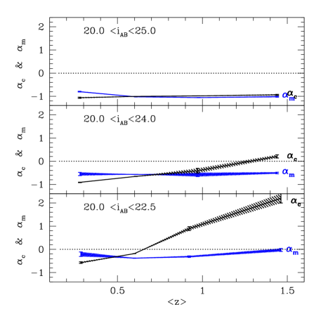
Figure 2: The magnification amplitude is proportional to the number counts slope $\alpha_{c}$ (black, defined in Eq. 11) and mean magnitude slope $\alpha_{\lambda}$ (blue, defined in Eq. 6), which are shown here as a function of the mean redshift of the source sample. Top panel corresponds to the main samples used in this paper ($20.0<I_{auto}<25.0$) for which the slopes are nearly constant (after photo-$z$ selection, see Fig. 1). For comparison, middle and bottom panels show the results for brighter samples (which we will also used in the test of Fig. 5) where the slopes can be closer to zero or positive.

We can now estimate the obscuration $A_{\lambda}^{*}$ in band $\lambda^{*}$ by combining $\Delta_{\lambda}^{*}$ and $\delta_{G}$:

$$A_{\lambda}^{*}={2.5\over{\ln 10}}\left[{\alpha_{c}\over{\alpha_{\lambda}^{*}}}\Delta_{\lambda}^{*}-\delta_{G}-Bn_{G}^{2.15}\right]$$ (15)

where $\lambda^{*}$ correspond to the band where the (flux limited) sample is selected. For other bands $\lambda$:

$$A_{\lambda}=A_{\lambda}^{*}+\Delta_{\lambda}-{\alpha_{\lambda}\over{\alpha_{\lambda}^{*}}}\Delta_{\lambda}^{*}$$ (16)

Magnification can then be found as:

$$\delta_{\mu}={\Delta_{\lambda}^{*}\over{\alpha_{\lambda}^{*}}}+A_{\lambda}^{*}{\ln 10\over{2.5}}$$ (17)

In our analysis we will select samples with $\alpha_{c}\simeq\alpha_{\lambda}^{*}\simeq-1$, for which $\delta_{\mu}\simeq-\delta_{G}$ as obscuration only affects fluxes (i.e. $\Delta_{\lambda}^{*}$) and cancels out for counts.

Note that this estimator for $\delta_{\mu}$ only uses $\lambda^{*}$, the wavelength where galaxies are selected (which in our case is the $I_{auto}-band$). The other bands can not be used here because we have used the information to determine the size of the obscuration correction. To have separate estimates of magnification from different bands we need to combine flux and counts estimates of galaxies selected in the different bands. Here we only consider the $i-band$ selection because we are using the publicly available COSMOS 30-band catalog of Ilbert et al. (2009), which is only provided in the $i-band$ selection. But, we will show results for the obscuration in several bands to see how important this effect is as a function of wavelength. To be able to select in other bands we would need PSF corrected total magnitudes and a catalog that is uniform in that band.

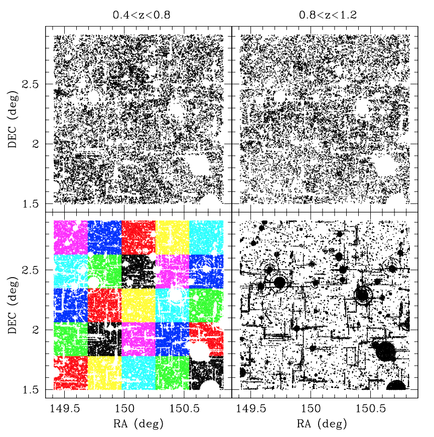
Figure 3: Galaxy positions of the $I_{auto}<25.0$ COSMOS samples used in this paper: lenses $0.4<z<0.8$ (top left) and sources $0.8<z<1.2$ (top right). For flux measurements we use different bands: U, B, G, V, R, I, Z and K as given in the public version of the COSMOS catalog of Ilbert et al. (2009). Bottom left panel shows the random catalogs with different colors for each of the 25 jack-knife regions. Bottom right panel shows the mask.

2.6 Cross-Correlations

As mentioned previously, we can not estimate the effects of magnification directly from $\delta m$ in Eq. 3 or $\delta_{G}$ in Eq. 9 for lens galaxies because we do not know the intrinsic fluxes or intrinsic counts before magnification or obscuration. Instead, we can estimate an average value for a population of lenses by comparing to the mean in a given galaxy selection: $\Delta_{\lambda}$ in Eq.4 or $\delta_{G}$ in Eq.12.

To estimate the population values $\Delta_{\lambda}$ and $\delta_{G}$ we stack the background observables (i.e.sources, labeled as $j$) around the foreground galaxy (i.e. lenses, labeled $i$) positions:

$$<\delta_{G_{i}}\delta_{G_{j}}>(\theta) = \frac{1}{\sum_{i,j}1}\sum_{i,j}\delta_{G_{i}}\delta_{G_{j}}$$

$$<\delta_{G_{i}}\Delta_{\lambda_{j}}>(\theta) = \frac{1}{\sum_{i,j}1}\sum_{i,j}\delta_{G_{i}}\Delta_{\lambda_{j}}$$ (18)

binned as a function of the $(i,j)$ pair separation $\theta$, the radius of an annulus $d(i,j)\in\theta\pm d\theta$. We estimate $\delta_{G}=n/\left<n\right>-1$ using uniform random (positions) catalogs (excluding masked and boundary regions, as shown in the bottom right panel of Fig. 3) to define the mean density $\left<n\right>$ that is available around each annulus. We also use random catalogs to estimate the mean magnitude $\bar{m}_{\lambda}\equiv<m_{\lambda}>$ in $\Delta_{\lambda}=m_{\lambda}-<m_{\lambda}>$ in each annulus. We assign magnitudes randomly from the real catalog to the random position catalog and this results in a mean that is independent of position.

The dominant contribution to the fluctuations $\Delta_{\lambda}$ and $\delta_{G}$ around each lens galaxy is not magnification, but the intrinsic clustering of galaxies. We can cancel this contribution by averaging over the full lens distribution, where we stack the background galaxies for all foreground galaxies. This is equivalent to doing the counts-counts cross-correlation. We have validated the cross-correlation results presented here against two independent cross-correlation codes over the same samples.

To interpret the results we assume that two samples are well separated in redshift space so that there is no intrinsic contribution to the cross-correlation from overlapping galaxies. This will be tested in §1.

3 DATA

We use the public COSMOS 30-band photometric redshift catalog of Ilbert et al. (2009) in the 2-deg² COSMOS field. We limit our study to $19<I_{auto}<25$ for both source and lensed samples, and to the 1.64 sq. deg region that overlaps with the HST-ACS catalog of Leauthaud et al. (2007) to identify potential blended objects. The results are robust to different sample selections which we have explored. We have not tried to optimize the sample selection to get better results, but rather use the simplest case to focus on the blending and obscuration effects. Fig. 3 shows the galaxy distribution in COSMOS catalog, the random catalogs, the jack-knife-regions and the mask that we have used. We split COSMOS in 5x5 grid regions (shown as color in the random catalog on the bottom left panel of Fig. 3) to use as jack-knife-regions for errorbar estimation (see Norberg et al. 2009). We use a conservative mask (bottom right panel in Fig. 3) to avoid impact of background light from star halos on galaxy photometry.

For flux measurements we use different bands: U, B, G, V, R, I, Z and K as given in the public version of the COSMOS catalog of Ilbert et al. (2009). For the i-band we use $I_{auto}$ which is a total magnitude corrected for PSF and provides a uniform selection (the parent sample was defined to a depth at least one magnitude deeper in $I_{auto}$-band ($I_{auto}<26$). For the other bands we use the fixed SUBARU aperture photometry provided in the catalog, which is optimal for photo-$z$ estimation, but non-optimal for magnification measurements. These are only used for the flux magnification and not for selection of the samples or estimating count fluctuations. The goal is to assess the importance of obscuration effects in different bands.

3.1 Photo-z selection and validation

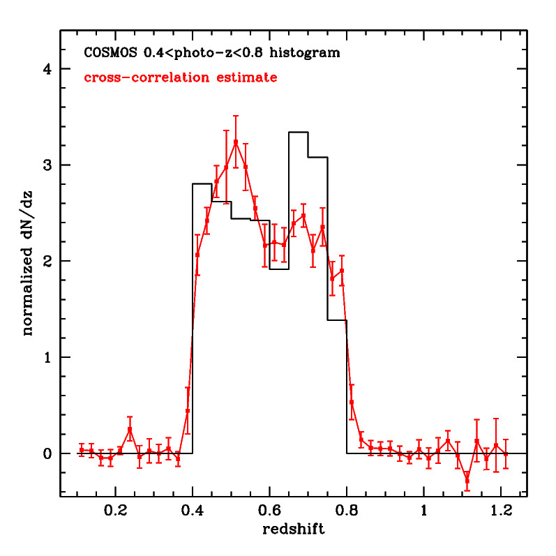
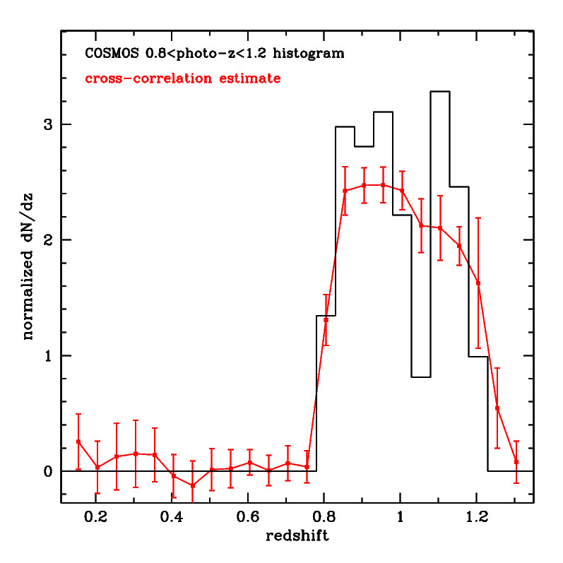
Figure 4: Comparison of redshift distributions from best photo-$z$ values (black histograms) and from cross-correlation with a spectroscopic sample from zCOSMOS (red lines and errorbars). Top panel corresponds to $0.4<z<0.8$ while bottom panel has $0.8<z<1.2$. Cross-correlation estimates of the bin N(z) are consistent with those of the high quality photo-$z$ binning.

We first explore the impact of photometric redshift errors on galaxy selection. Ideal samples would contain no overlap in redshift between the lens and source samples, as this overlap could include a small but significant auto-correlation signal that could contaminate the lensing measurement. In order to accomplish this sample separation we select only those galaxies which have $99\%$ of their individual PDF inside the chosen z-bin range. Figure 4 shows the density distribution $dN(z)/dz$ of best photo-$z$ values normalized to the total number of galaxies, and shows that the conservative 99% cut ensures that our lens and source bins are well separated. Table 1 shows statistics of these samples.

$z$-bin	$\left<z\right>$	$N_{g}$	$<I_{auto}>$	$\alpha_{c}/\alpha_{m}$	$n_{g}$
$z$ range	mean	$\#$	mag		$\#$/arcm2
0.4 - 0.8	0.61	23532	22.48		5.0
0.8 - 1.2	0.98	19581	23.10	-1.0/-1.0	4.1
stars		10088	21.98		2.2

Table 1: Background (sources) and foreground (lenses) samples used in this paper. Both samples have $19<I_{auto}<25.0$ and $99\%$ of each galaxy individual photo-$z$ pdf is within $z$ range. As a null test we also use a sample of stars in the foreground with same magnitude cuts. Stars are brighter and more sparse.

We validate the $dN(z)/dz$ estimates using cross-correlation with spectroscopic redshifts, following the technique described in Schmidt et al. (2013). We cross-correlate our 99% photometric redshift cut samples with spectroscopically confirmed galaxies from the final release of the zCOSMOS bright sample (Lilly et al. 2007). The validation is shown as lines with error-bars in Fig. 4. The top panel corresponds to $0.4<z<0.8$, while the bottom panel has $0.8<z<1.2$. By comparing the two panels we can see that there is little overlap between the two samples. As expected by our selection, the overlapping tails between bins are smaller than 1% which have negligible effects on the cross-correlation measurements, given our error-bars and the amplitude of the signal. Results are relatively insensitive to specific details of the redshift bin choice. We choose a z-bin width or $\Delta z=0.4$ in order to define a large enough sample to measure a significant correlation signal, and start at $z=0.4$ in order to define a sample with a substantial cosmological volume.

3.2 Cross-correlation validation

Here we test if our cross-correlation measurements are consistent with the weak lensing magnification signal.

We select three ($j=1,2,3$) different source galaxies (all within $0.8<z<1.2$) with $22.5<I_{auto}(1)<25.0$, $20<I_{auto}(2)<24.4$ and $20.0<I_{auto}(3)<24.0$ which have slopes: $\alpha_{c}=$-1.26, 0.01 and 0.38 and mean magnitudes $<I_{auto}>=$23.6, 23.0 and 22.7. We test if the cross-correlation with the same lens sample ($0.4<z<0.8$ as in Table 1) scales linearly with the number count slope $\alpha_{c}$, as expected from Eq. 11. This test is shown in Fig. 5, which displays the amplitude of the cross-correlation in the first angular bin (where S/N is largest) as a function of $\alpha_{c}$. The dashed line shows the prediction based on the first point: $\delta_{G}(j)=\alpha_{c}(j)/\alpha_{c}(1)~{}\delta_{G}(1)$ (with $\alpha_{c}(1)=-1.26$). There is a very good agreement, which indicates that the cross-correlation signal is consistent with the weak lensing magnification effect. Note in particular the null test (middle point) where we find no cross-correlation for $\alpha_{c}\simeq 0$, as expected. Brighter fluxes give larger slopes (see Fig. 2), but they also include fewer galaxies and larger cross-correlation errors (because of the small area of COSMOS), so this regime has lower S/N and is more difficult to test with COSMOS.

Figure 5: Amplitude of counts cross-correlation at small scales ($0.03<\theta_{12}<0.09$ arcmin) between a lens sample at $0.4<z<0.8$ and a source sample at $0.8<z<1.2$ as a function of $\alpha_{c}$. Each point corresponds to one in three ($j=1,2,3$) different magnitude cuts ($<I_{auto}(j)>=$23.6, 23.0 and 22.7) which result in $\alpha_{c}(j)=$-1.26, 0.01 and 0.38. The dashed line is the prediction in Eq.11 based on the first measurement. The scaling with $\alpha_{c}$ agrees well with that expected for weak lensing magnification.

4 Results

In this section we apply the methodology presented in section 2 to the COSMOS samples defined in section 3. The goal is to combine the two cross-correlation signals from fluxes and counts to estimate the obscuration effects and recover a cross-correlation signal that is consistent with the magnification effect. We then estimate the mass profiles of the lenses and compare the results with simulations. We end with a comparison of the corresponding profiles obtained using tangential shear and flux-size magnification for the same lenses.

4.1 Raw cross-correlations

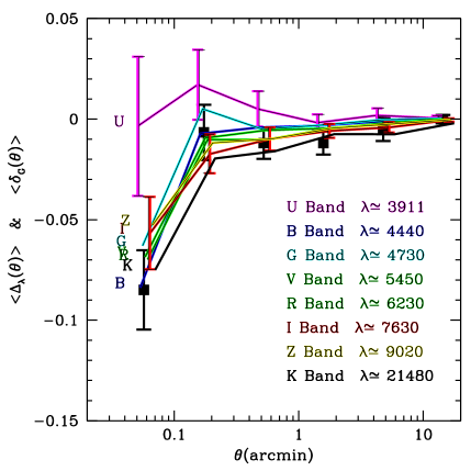
Figure 6: Source counts fluctuations $\left<\delta_{G}\right>$ (filled squares) and magnitude differences $\left<\Delta_{\lambda}\right>$ in different bands (color lines) for galaxy sources ($0.8<z<1.2$) around galaxy lenses ($0.4<z<0.8$) in circular annulus of mean radius $\theta$. For clarity we only show errors for counts and for K, I, and U bands (black, red, and purple lines). These are the raw cross-correlations without any correction for obscuration effects or scaling by slopes. Except for the U-band, all estimates seem to be consistent with each other.

We first present here the raw cross-correlation results without any corrections. The angular cross-correlation of density fluctuations $\left<\delta_{G}\right>$ and magnitude fluctuations $\left<\Delta_{\lambda}\right>$ in several bands $\lambda$, as detailed in Section §2.6. We use six angular bins, which are uniform in log space in the range: $0.03<\theta<30$ arcmin, but results are similar, within errors, for different bins. Errors are estimated using the jack-knife samples, as explained in section 3. Fig. 6 compares the raw source count fluctuations and magnitude differences of sources around lenses, i.e. $\left<\delta_{G}\right>$ and $\left<\Delta_{\lambda}\right>$ in §2.6, using different bands: U, B, G, V, R, I, Z and K for $\lambda$.

Because in our case $\alpha_{c}\simeq\alpha_{\lambda}\simeq-1$ we can already see here that there is a good agreement between the magnification signal from counts and flux for most of the bands. This is a good internal consistency check and shows that we can use different bands to estimate magnification. The U-band shows the biggest outlier, indicating that is more affected by systematic effects (see below).

As a null test, we have also cross correlated the stellar counts and magnitude fluctuations around the same lenses. In this case the errors are only slightly larger because there are only $N=10088$ stars in the sample (with same magnitude cuts as for galaxies) with a mean magnitude of $\left<I_{auto}\right>=21.98$ compared to $\left<I_{auto}\right>=23.10$ in the galaxy sources. Within errors there is no signal in the stars counts or fluxes, as expected (see dashed line in Fig. 8). This already indicates that obscuration (or merging) errors are not large, as compared to errorbars, at least for the brighter stellar sample.

4.2 Effects of obscuration and blending

From the above raw cross-correlations we can use the formalism presented in Section 2 to estimate the obscuration effect $A(\Lambda)$ from comparing the average flux to the average counts around lenses. We estimate the obscuration for each jack-knife region and use it to estimate the errors as detailed in section 3. The top panel of Fig. 7 shows the obscuration correction $A(\lambda)$ using Eq. 16, which combines the effects of counts and magnitudes to separate obscuration from magnification. Recall that the values of $A(\lambda)$ have units of magnitudes. We can see that these corrections are small (less than 0.1 mag) but significant and need to be taken into account for accurate magnification estimates.

The general trend shown in Fig. 7 is that obscuration is consistent with extinction in that is larger for bluer bands and close to zero for reddest bands. But there are exceptions to this (e. g. the B-band) so that we can not exclude that some of these trends are due to other systematics.

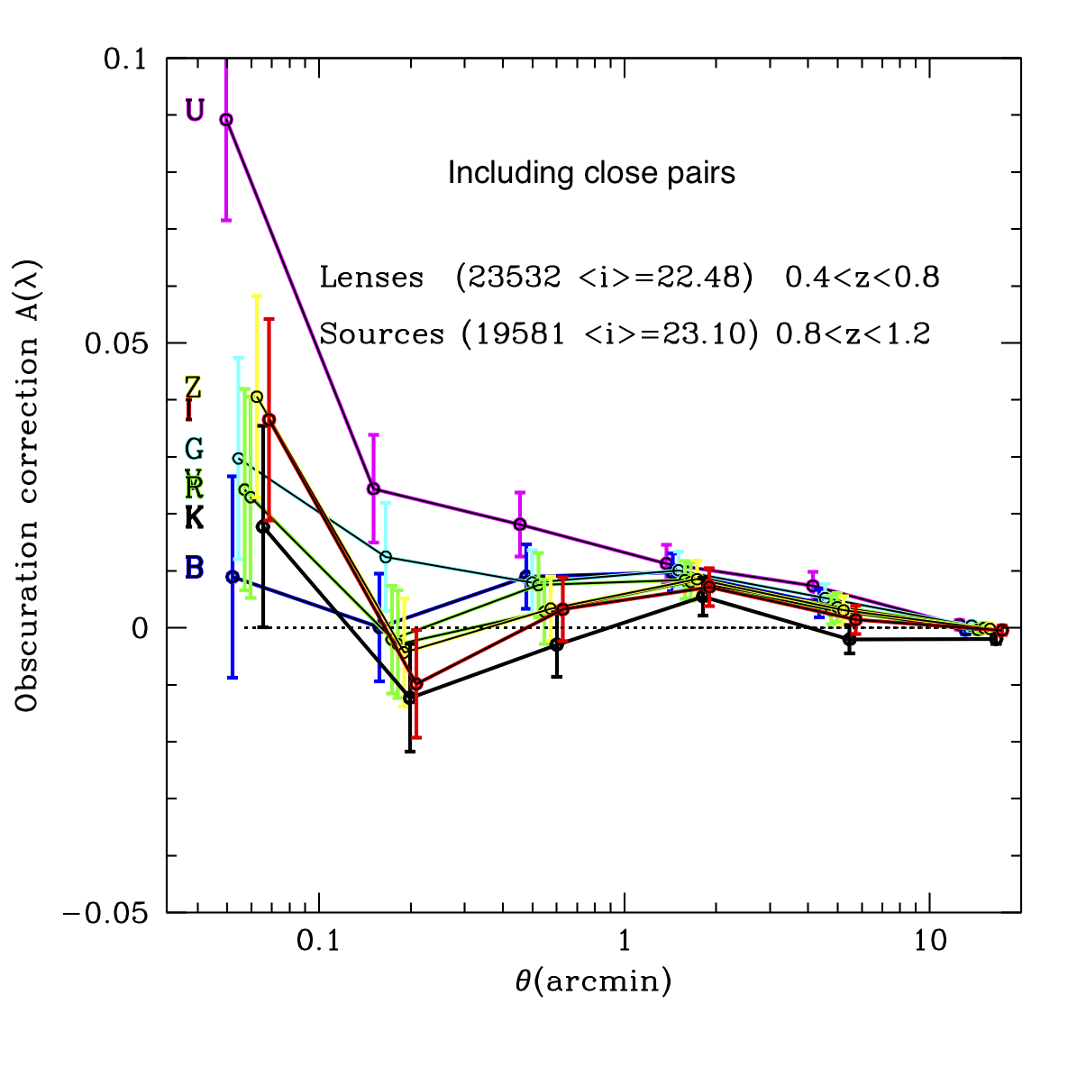
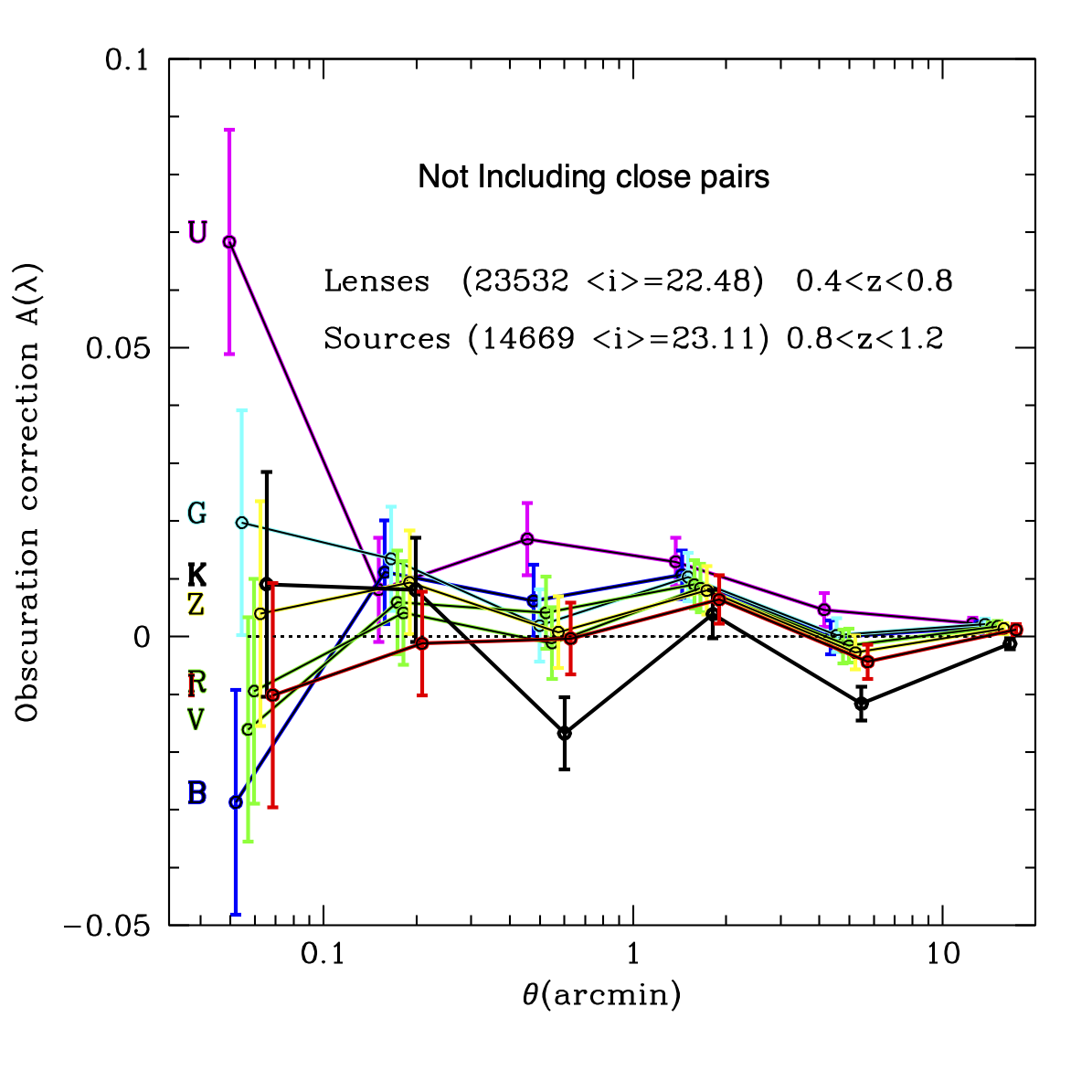
Figure 7: Obscuration correction (from Eq. 16) for different bands $\lambda$ when galaxies are selected in the I-band. Color coding is as in Fig. 6. The top panel include all galaxies, while the bottom panel exclude pairs that are too close (potential blends). Blending effects are important (up to 0.04 mag obscuration) at angular scales smaller than a few arcsec, but errors are too large to characterise this effect with confidence as a function of $\lambda$.

The bottom panel of Fig. 7 shows the same obscuration correction when we remove from the sample objects that are potential blends (galaxies in close pairs, separated by $\theta<1$ arcsec according to ACS-HST measurements, see §2.4). The number of pairs is slightly reduced, which increases the uncertainties, however, the size of the errorbars does not increase much. In general, we can see that when using all galaxies, there is obscuration for all bands on the smallest scales, while this tendency tends to disappear when we remove the potential blends (with the exception of the U-band). This indicates that blending is playing some role in the obscuration signal and can not be ignored, even for our sample which is relatively bright on average because of the photo-$z$ selection ($<I_{auto}>\sim 23.1$, see Table 1).

We can see this tendency more clearly when we focus in the I-band case in Fig. 8. The correction for the I-band, which is the one most relevant for our magnification estimation, is consistent with zero at large scales but is significantly different from zero at the smallest scales. After removing the potential blends (bottom panel) there is no significant obscuration correction.

The black lines show the mean corrected values for all galaxies, while the red lines (which lies just on top) shows the results without the average blending subtraction in Eq. 13

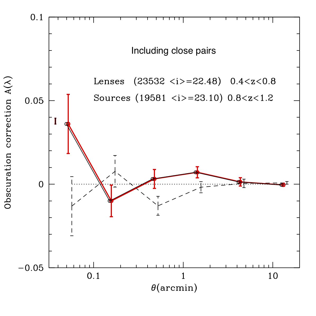
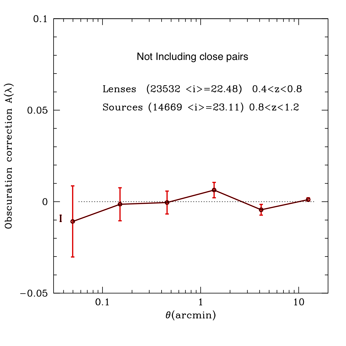
Figure 8: Obscuration correction for the I-band (i.e. one of the curves in Fig.7). The top panel includes all galaxies, while the bottom panel excludes pairs that are too close (potential blends). The dashed line in the top panel shows the corresponding obscuration correction when using the foreground stars in the field instead of the galaxy sources. Obscuration correction is significant for galaxies, but it is negligible after removing the potential blends (bottom panel).

The dashed line in the top panel of Fig. 8 shows the corresponding obscuration correction when we use stars instead of galaxies to correlate around the same lenses. This test indicates that the obscuration correction is negligible for stars, which could be explained by the fact that the stellar sample is over one magnitude brighter than the galaxy sample and their cross-correlation is negligible, as mentioned in previous section. Note that we are masking the area around bright stars with data reduction flags which also reduces the potential contamination in stars. We also note that de-blending effects in data reduction apply differently for stars and galaxies.

4.3 Magnification estimates

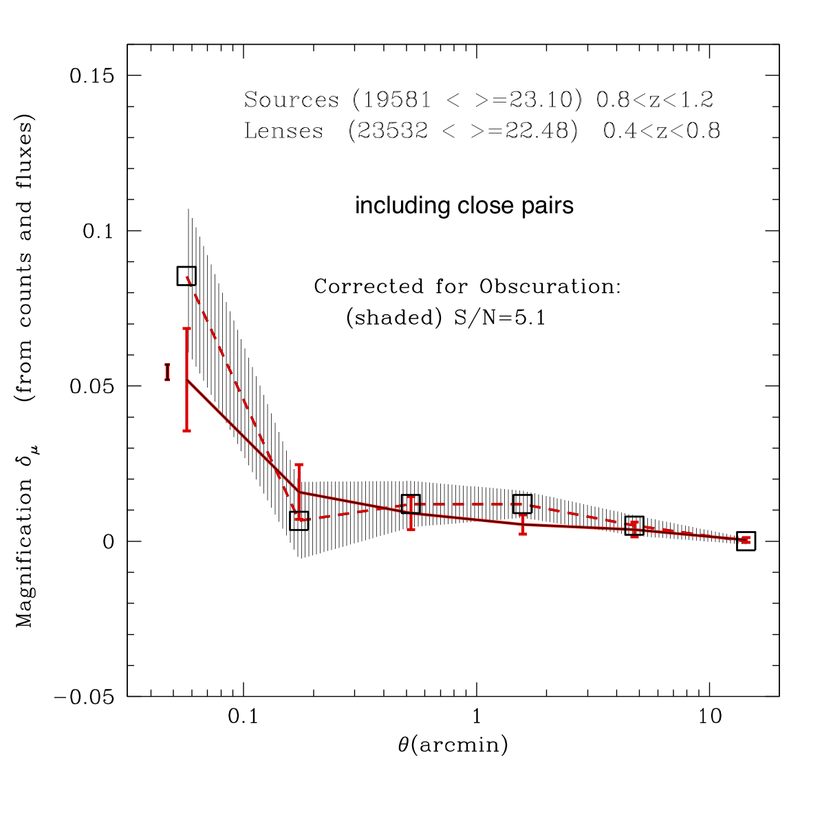
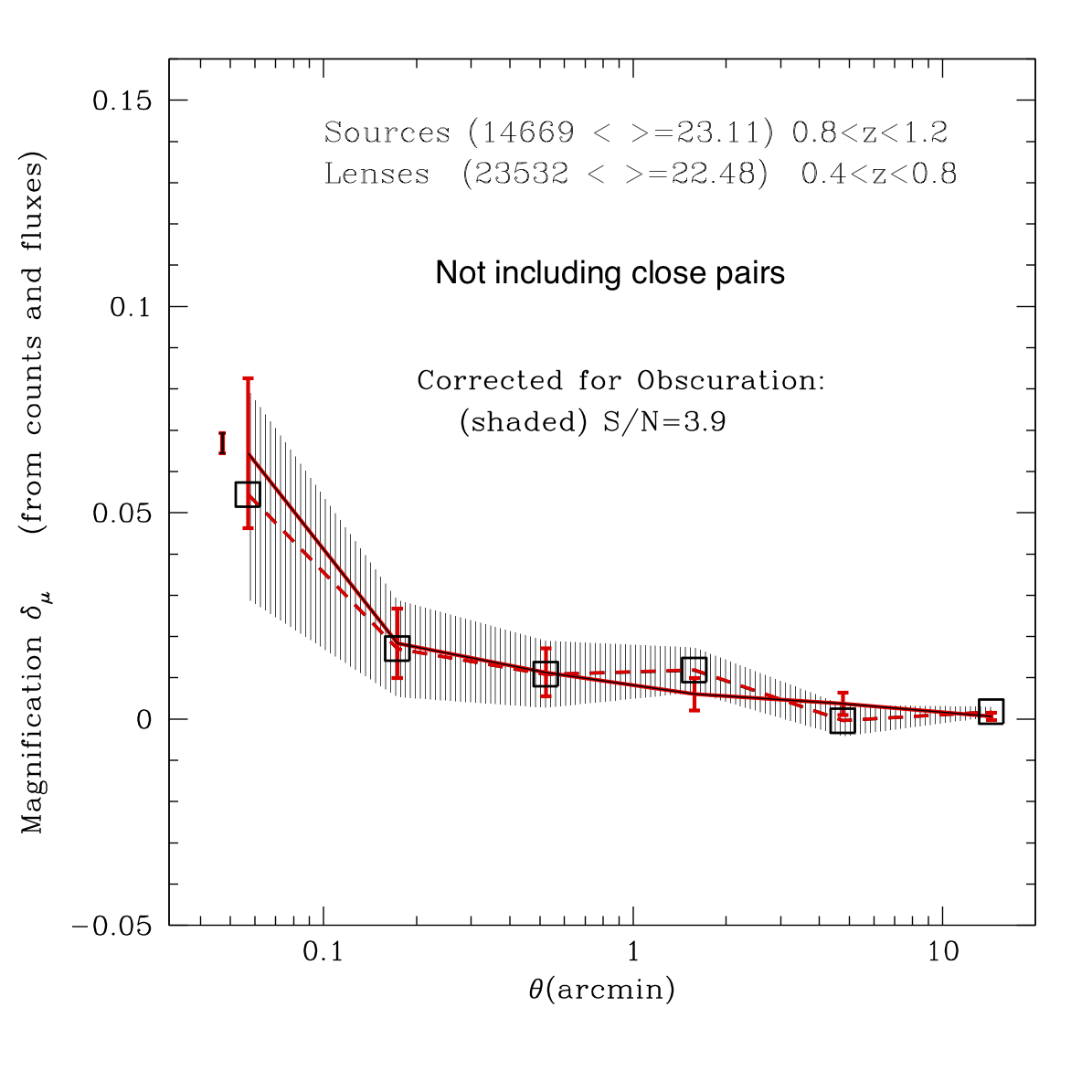
Figure 9: Magnification with obscuration correction (shaded region with dashed line) in the i-band as compared to the magnification estimate without any correction from counts (squares) and from magnitudes (continuous lines). The top panel includes all objects. In the bottom panel we remove potential blends (close pairs in HST images). Removal of the close pairs does not cause a statistically significant shift in the measurement. Small scales have the highest S/N, but obscuration is also largest at these scales, see Fig.7-8.

After obtaining the obscuration correction in previous sub-section, we now use it to recover the magnification signal combining flux and counts in the i-band. We estimate the magnification for each jack-knife region and use the variance of the 25 jack-knife regions to estimate the errors. Fig. 9 shows the magnification estimates with obscuration correction in Eq. 17 (shaded region) and without corrections (lines and points), i.e. scaled by the corresponding slopes $\alpha_{c}$ and $\alpha_{\lambda}$. The grey dashed line shows the mean corrected values for all galaxies, while the red dashed (which lies just on top of the grey line) shows the results without the average blending subtraction in Eq. 13. As mentioned before this term is negligible for our sample. But this does not mean the blending (or associated data reduction effects) can not cause obscuration effects, as indicated in Fig. 7-8.

Magnification from I-band flux has higher signal-to-noise than from I-band counts, though both measurements are consistent after we include the obscuration correction, which only degrades the S/N slightly with respect to the uncorrected flux estimate.

The bottom panel of Fig. 9 shows the same results when we remove pairs that are potential blends (i.e. galaxies that have pairs closer than $\theta<1$ arcsec according to the ACS-HST). Close pairs are only present in the source galaxies sample ($0.8<z<1.2$). There are no close pairs in the lens sample ($0.4<z<0.8$) as the corresponding physical scales are smaller and the sample contains brighter galaxies (see Table 1). The number of sources is reduced from 19581 to 14669. Removing potential blends reduces the magnification signal (and the $S/N$) by about $\sim 30\%$. Removing the close pairs results in measurements that fall within the 1-sigma uncertainties, showing that the close pairs are not having an appreciable impact on the magnification measurement. However, out of an abundance of caution we remove close pairs in our calculations to avoid any potential systematic effects. In next sub-section, we use it to estimate matter profiles and compare to other results.

4.4 Matter profiles

The gravitational lensing effect is proportional to the projected mass density $\Sigma$, which on small scales is typically dominated by the surface density of a single dark matter halo, which acts as a lens:

$$\delta_{\mu}(\theta)\simeq 2~{}\kappa(\theta)\simeq 2~{}{\Sigma(\theta)\over{\Sigma_{c}}}$$ (19)

The weight, $\Sigma_{c}$, depends on the critical density $\rho_{c}$ and the lensing geometry, but is independent of wavelength $\lambda$:

$$\Sigma_{c}={c^{2}\over{4\pi G}}{\chi_{j}\over{\chi_{i}\chi_{ij}}}={2\over{3}}{\chi^{2}_{H}\chi_{j}\over{\chi_{i}\chi_{ij}}}\rho_{c}$$ (20)

where $\chi_{H}\equiv c/H_{0}$ and $\chi_{i}$, $\chi_{j}$, $\chi_{ij}$ refers to the comoving distance to the lenses, to the sources and between them.

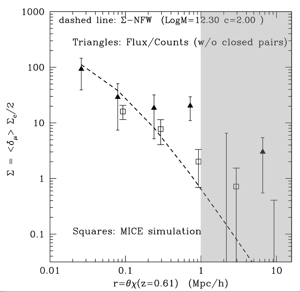
Figure 10: Projected mass $\Sigma=\delta_{\mu}\Sigma_{c}/2$ from flux/counts magnification without close pairs (triangles) compared with results from the MICE simulations (squares). Dashed line shows the NFW 1-halo with $M_{200}\simeq 2\times 10^{12}M_{\sun}h/pc^{2}$ and $c=2$. The mean simulation results show a clear (and significant) excess above the NFW profile on the largest scales, indicating the presence of a 2-halo term. The data is consistent with the 1-halo term on small scales ($<0.5$ Mpc/h) but are too noisy in the 2-halo scales (shaded region) because of the small size of the COSMOS field.

Closed triangles in Fig. 10 show the mass profile (in comoving coordinates $r=\chi_{i}\theta$) inferred from the magnification measurement $\delta_{\mu}$ (shown in bottom panel Fig. 9) using the following relation:

$$\Sigma(r)=\delta_{\mu}(\theta)~{}\Sigma_{c}/2$$ (21)

We estimate the mass profile for each jack-knife region and use the variance of the 25 jack-knife regions to estimate the errors. Fitting a power law to the triangles in Fig. 11 we find a mean amplitude of dark matter projected mass $\Sigma=25\pm 6M_{\sun}h/pc^{2}$ at comoving radius of 0.1 Mpc/h. The dashed line shows the 1-halo NFW profile with concentration $c=2$ that best matches this profile. We fit the first 3 points because the NFW is too steep to fit the measured profiles and we only expect the 1-halo term to dominate in the smallest scales. On larger scales ($>0.3Mpc/h$) the magnification measurements show marginal evidence for an up-turn (above the 1-halo term) which could be related to the 2-halo term. However, note that the 3 last points in the profile are consistent with zero at a 2-sigma level of significance.

Our flux limited (photo-$z$ selected) lenses have $<I_{auto}>\simeq 22.5$ at $<z>\simeq 0.61$ (see Table 1). This corresponds to a k-corrected absolute magnitude of $M\simeq-21$ which matches a NFW profile with mass of $M_{200}\simeq 2\times 10^{12}M_{\sun}h/pc^{2}$ and $c=2$.

4.5 Comparison with simulations

We utilize simulations to validate our method, to test the error estimation and to compared the mass profile estimates with the LCDM model. We use the MICE simulations (Fosalba et al. 2015a, Crocce et al. 2015, Fosalba et al. 2015b, Carretero et al. 2015, Hoffmann et al. 2015), which include the magnification effect both in magnitudes and positions (see Section 5 and Fig.14 in Fosalba et al. 2015b). In the simulations we use true cosmological redshifts instead of photometric redshifts, as the photometric redshift effects is already tested in Section 3.2. We first limit the simulations to $19<I_{auto}<25$. To include the same galaxy selection in the simulation as in the samples of Table 1, we draw objects randomly from the simulation to have the same $I_{auto}$ magnitude distribution in steps of $\Delta z=0.01$ and $\Delta I_{auto}=0.01$.

Fig. 10 shows as squares the results in the simulation. Here we show the $\Sigma$ measurements from the galaxy-magnitude cross-correlations for galaxies selected in a similar way as in Table 1. Mass profiles in the simulation are only reliable for scales larger that $\simeq 0.1$ Mpc/h because of resolution effects (particle mass is $\simeq 3\times 10^{10}M_{\sun}/h$ and $l_{soft}=50$ kpc/h).

Error bars on the the square points in Fig. 10 are derived from a set of 50 separate COSMOS-sized regions (of $\simeq 1.7$ deg² and using the same mask as used in this paper, see Fig. 3). We can see that the simulation errors are comparable to the jack-knife errors in the COSMOS galaxies. We do not expect these errors to be identical because jack-knife errors are only approximate and the simulations are not realistic in the obscuration effects, photometric errors or the photo-$z$ performance.

The MICE simulations follow a similar NFW profile as data at small scales. But note the systematic differences above $\simeq 1$ Mpc/h due to the 2-halo term. Even when the simulation errors shown are large, because they correspond to the COSMOS area, the mean simulated values have a much smaller error, as they come from 50 times larger area. Deviations from NFW seem larger in the real data than in the simulations, but as mentioned above, these differences are not significant at the 2-sigma level in the data. Moreover, the sampling variance errors in the simulation indicate that the COSMOS field is too small to provide a detection above $\simeq 1$ Mpc/h scales.

4.6 Comparison with tangential shear

With the results from the previous sections, we can now ask the question: are mass profiles estimated from magnification consistent with those derived from shear? We measure differential mass profiles, $\Delta\Sigma$, from tangential shear $\gamma_{t}$ around the same lenses (see Schmidt et al. 2012):

$$\Delta\Sigma(\theta)\equiv\Sigma(<\theta)-\Sigma(\theta)=~{}\gamma_{t}(\theta)~{}\Sigma_{c}$$ (22)

We then use the shear measurements of Leauthaud et al. 2007 to estimate tangential shear average over the same lenses (from sources in Schmidt et al. 2012). The result is shown in Fig. 11. Profiles are shown as a function of comoving radius: $r=\theta\chi$ Mpc/h, where $\chi$ is the comoving distance to $z=0.61$, the mean redshift of the lenses, and $\theta$ is the measured angular separation. To compare both profiles we show $\Sigma$ (dashed line) and $\Delta\Sigma$ (continuous line) for the same NFW profile (with $c=2$ and $M_{200}\simeq 2\times 10^{12}M_{\sun}h/pc^{2}$). We see how both measurements give similar profiles for the smallest comoving scales ($r<0.3Mpc/h$). Our measurements from flux/counts (triangles) show a flatter profile, possibly due to the 2-halo term (see Fig. 10), while the tangential shear measurements seem to follow the 1-halo term. Note that $\Delta\Sigma$ in Eq.22 is in general less sensitive to the 2-halo term than $\Sigma$ because the former is cumulative. However, the systematics for $\Delta\Sigma$ and $\Sigma$ are different.

Our results for the 2-halo term (shaded region Fig. 11) in are not conclusive. Recall that the NFW profile shown was fitted to the three smallest scale points in $\Sigma$, which could bias this interpretation. The shear values could also be subject to some uncorrected shape biases. But note that magnification measurements have low significance on scales larger than $\simeq 1$ Mpc/h (see Fig.10) and we need larger areas to be able to make a more detailed comparison on the 1-halo to 2-halo term transition.

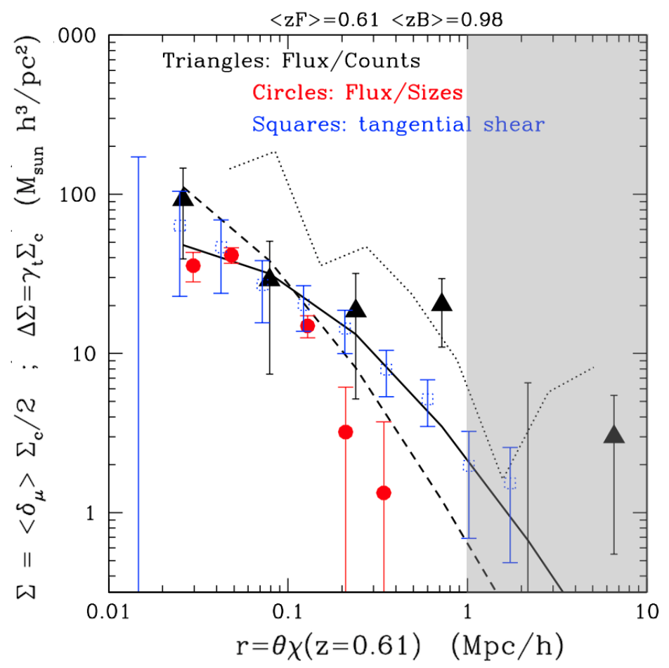
Figure 11: Projected mass $\Sigma=\delta_{\mu}\Sigma_{c}/2$ from magnification in flux/counts (black triangles) compared to that from flux/sizes (red circles) and $\Delta\Sigma$ from tangential shear (blue squares with errorbars), all over the same galaxy lenses (first raw in Table 1). The different methods agree well with each other and with the NFW predictions for $\Sigma$ (dashed line) and for $\Delta\Sigma$ (continuous line) with $M_{200}\simeq 2\times 10^{12}M_{\sun}h/pc^{2}$ and $c=2$. Shaded region correspond to scales that are too noisy for the area of the COSMOS field. The dotted line shows $\Sigma$ from Flux/sizes in galaxy groups (Schmidt et al. 2012). The group profile has similar shape to that of individual galaxies, but a factor of 4-8 larger amplitude for the density profiles, as expected.

4.7 Comparison with flux/size and group profiles

In addition to changing the flux of galaxies, magnification ($\mu$ in Eq.1) also changes their apparent size (e.g. Bartelmann & Narayan 1995, Bartelmann & Schneider 2001). In this work, we have, to this point, not used measured galaxy sizes, but this information is available in the parent COSMOS catalog. We estimate mass profiles for the same lens sample (first row in Table 1) with the method presented by Schmidt et al. (2012) which combines flux and size magnification. This method has its own potential systematics which are discussed in Schmidt et al. (2012) and are not addressed here.

Is the flux-counts magnification signal consistent with the flux-size magnification signal? Red circles in Fig. 11 show the mass profiles estimated with flux-size measurements using the method presented in Schmidt et al. (2012), over the same sample of lenses used in this paper. There is good agreement with the profiles from our flux-counts magnification estimates on the smallest scales. On the largest scales, measurements have low significance and the flux-size measurements don’t provide a detection. At 2-sigma level both results are consistent. We also plot as dotted line the flux-size measurements for galaxy groups in Schmidt et al. (2012). As expected the group estimates are larger: $\Sigma\simeq 100-200M_{\sun}h/pc^{2}$ at comoving radius of 0.1 Mpc/h, four-eight times larger than for flux limited galaxies ($<M_{i}>\simeq-21$ at $z\simeq 0.6$).

5 Conclusions & Discussion

We have studied magnification with the COSMOS photo-$z$ Survey to $I_{auto}<25.0$ both with galaxy densities and fluxes (magnitudes). We take advantage of the good photo-$z$ characterization to split foreground ($0.4<z<0.8$) and background ($0.8<z<1.2)$) galaxies into contiguous redshift bins using photo-$z$ selection with 99% CL. We estimate the redshift distribution $N(z)$ from cross-correlation with zCOSMOS spectroscopic sample and find good agreement with the 99% photo-$z$ selection.

We introduce a formalism to account for systematic obscuration effects (i.e. not due to magnification) in the fluxes by combining counts and magnitudes. We find that obscuration effects are typically smaller than $0.05\ mag$ at all scales when galaxies are selected in the COSMOS $I_{auto}$ band, but they need to be taken into account given the errorbars. The general trend of obscuration is consistent with extinction in that is larger for the U band and consistent with zero for the reddest bands. On the smallest scales, where our results are more significant, this obscuration reduces significantly when we remove close pairs. This indicates that blending effects have an important impact ($\simeq 30\%$) in our magnification signal.

We measure a significant ($S/N\simeq 3.9$) magnification signal that is consistent for counts and magnitudes. We use these measurements to estimate the matter mass profiles of regular (flux limited) ($<I_{auto}>\simeq 22.48$) galaxies at redshift $z\simeq 0.61$ ($<M_{i}>\simeq-21$). We find a mean amplitude of dark matter projected mass $\Sigma=25\pm 6M_{\sun}h/pc^{2}$ at comoving radius of 0.1 Mpc/h, which is consistent with a NFW type profile ( $M_{200}\simeq 2\times 10^{12}M_{\sun}h/pc^{2}$ and concentration of $c=2$ ) on scales $\simeq 30-300$ Kpc/h and shows marginal evidence of 2-halo term at larger scales, up to 10 Mpc/h. We compare these results with simulations and shear profiles (for the same lenses) which agree on small scales.

As shown in Fig. 8 and Fig. 9 blending effects start to be important (up to a factor of $0.04~{}mag$ obscuration) at angular scales smaller than a few arcsec. But, due to the small area of the COSMOS field, errors are too large to characterize this effect with confidence. Extinction and other systematic obscuration effects can be as large as 0.1 mag but are typically smaller than 0.02 mag depending on the band (see Fig. 7). These effects can quickly become more important for deeper samples, such as the deepest samples expected from the LSST survey (but not in the LSST Gold Sample).

Results in this paper are a proof of concept for magnification measurements using only galaxy counts and fluxes. We have not tried to optimize choices, such as sample selection, redshift binning or use of weights because the COSMOS field is too small to provide significant statistics. Looking ahead, these methods are now being tested over wider areas ($\simeq 50-100$ deg2) with accurate photo-z, such as those in the PAU Survey (Eriksen et al 2019). As the statistical errors reduced, we will need better control of systematic effects and to explore ways to optimize our estimates. In the near future we expect these methods to mature and to be applied to the much deeper and wider (18,000 deg2) LSST samples. The COSMOS statistical errors presented in this paper should decrease by a factor of $\sqrt{10,000}\simeq 100$ for LSST, at the price of having a less accurate photo-z estimation. The challenge then will be to have a better control of photometric and photo-z error uncertainties. Results with better photo-z precision from the smaller area surveys can then be used to help calibrate some of these uncertainties. Besides the methods explored in this paper to mitigate systematic effects, we should also use image simulations: embeding fake objects (with known properties) in real imaging to accurately characterize measurement biases (e.g. see Suchyta et al. 2016, Garcia-Fernandez et al. 2018).

We conclude that magnification from counts and fluxes using photometric redshifts in flux limited galaxy samples has the potential to provide accurate weak lensing measurements in future wide field surveys once we carefully take into account systematic effects, such as obscuration and blending. These weak lensing measurements can be complementary (compared to cosmic shear and size magnification) for the deeper samples.

Data Availability Statement

The data and codes used in this article will be shared on reasonable request to the corresponding author.

References

- (1) Abbott, T.M.C., et al. 2018, Phys. Rev. D, 98, 043526
- (2) Bartelmann, M., & Schneider, P. 2001, Phys.Rep., 340, 291
- (3) Bartelmann, M., & Narayan, R. 1995, ApJ, 451, 60
- (4) Bauer, A. H., Gaztanaga, E., Marti, P., Miquel, R. 2014, MNRAS, 440, 3701
- (5) Bernstein, G. M., & Cai, Y.C., 2011, MNRAS, 445, 2825
- (6) Carretero, J., , Castander, F. J., Gaztanaga E. , Crocce, M. & Fosalba, P., 2015, MNRAS, 447, 646
- (7) Carretero, J. et al., 2017, Proceedings, 2017 European Physical Society Conference on High Energy Physics (PoS, EPS-HEP2017), 488
- (8) Cai, Y.C. & Bernstein, G. M., 2011, MNRAS, 445, 2825
- (9) Chang C. et al., 2015, ApJ, 801, 73
- (10) Crocce, M. Castander, F. J., Gaztanaga E., & Fosalba, P., 2015, MNRAS, 453, 1513
- (11) Jee, M. J., et al., 2012, ApJ, 765, 26
- (12) Dawson, W. A., et al., 2016, ApJ, 816, 11
- (13) Eriksen, M. & Gaztanaga, E., 2015a, MNRAS, 451, 1553
- (14) Eriksen, M. & Gaztanaga, E., 2015b, MNRAS, 452, 2149
- (15) Eriksen, M. & Gaztanaga, E., 2015c, MNRAS, 452, 2168
- (16) Eriksen, M. & Gaztanaga, E., 2018, MNRAS, 480, 5226
- (17) Eriksen, M. et al., 2019, MNRAS, 484, 4200
- (18) Ford, J., et al., 2015, MNRAS, 447, 1304
- (19) Fosalba, P., Crocce, M. Gaztanaga, E., & Castander, F. J., 2015a, MNRAS, 448, 2987
- (20) Fosalba, P., Gaztanaga, E., Castander, F. J., & Crocce, M. 2015b, MNRAS, 447, 1319
- (21) Garcia-Fernandez, M., 2018, MNRAS, 476, 1071
- (22) Gaztanaga, E., 2003, ApJ, 589, 1
- (23) Gaztanaga, E., Eriksen, M., Crocce, M., Castander, F., Fosalba, P., Marti, P., Miquel, R. and Cabre, A. 2012, MNRAS, 2904
- (24) Heymnans, C., et al., 2013, MNRAS, 432, 2433
- (25) Hikage, C. et al. 2019 PASJ, 71, 43.
- (26) Hildebrant, H. et al. 2009 A&A, 507, 683.
- (27) Hildebrant, H., et al., 2016, MNRAS, 455, 3943
- (28) Hildebrant, H., et al., 2017, MNRAS, 465, 1454
- (29) Hoffmann K., Bel J., Gaztanaga E., Crocce M., Fosalba P., & Castander F.J., 2015, MNRAS, 447, 1724
- (30) Ilbert, O., Capak, P., Salvato, M., et al. 2009, ApJ, 690, 1236
- (31) Leauthaud, A., Massey, R., Kneib, J.-P., et al. 2007, ApJS, 172, 219
- (32) Lilly, S.J. et al. 2007, ApJS, 172, 70
- (33) LSST Science Book, arXiv:0912.0201
- (34) Narayan, R. 1989, ApJ, 339, L53
- (35) Norberg, P., Baugh, C. M., Gaztanaga, E., & Croton, D. J. 2009, MNRAS, 396, 19
- (36) Ménard, B., Scranton, R., Fukugita, M., & Richards, G. 2010, MNRAS, 405, 1025
- (37) Morrison, C.B., Scranton, R., Ménard, B., Schmidt, S. J., Tyson, J.A., Ryan, R., Choi, A., Wittman, D.M. 2012, MNRAS, 426, 2489
- (38) Schmidt, S. J., Ménard, B., Scranton, R., Morrison, C., & McBride, C. K. 2013, MNRAS, 431, 3307
- (39) Schmidt, F., Leauthaud, A., Massey, R., et al. 2012, ApJL, 744, L22
- (40) Schneider, P. 1987 ApJ, 319, 9
- (41) Scranton et al. 2005 ApJ, 633, 589
- (42) Suchyta, E., et al., 2016, MNRAS, 457, 786
- (43) Van Waerbeke, L., et al., 2010, ApJ, 723, 13
- (44) Wittman D. M., et al., 2002, in Tyson J. A., Wolff S., eds, Society of Photo-Optical Instrumentation Engineers (SPIE) Conference Series, Vol. 4836, pp. 73-82
- (45) Weinberg, D., et al., 20, 2013, Phy. Rep. 530, 87