A Least-Squares Formulation of the Moving Discontinuous Galerkin Finite Element Method with Interface Condition Enforcement

Abstract

A least-squares formulation of the Moving Discontinuous Galerkin Finite Element Method with Interface Condition Enforcement (LS-MDG-ICE) is presented. This method combines MDG-ICE, which uses a weak formulation that separately enforces a conservation law and the corresponding interface condition and treats the discrete geometry as a variable, with the Discontinuous Petrov-Galerkin (DPG) methodology of Demkowicz and Gopalakrishnan to systematically generate optimal test functions from the trial spaces of both the discrete flow field and discrete geometry. For inviscid flows, LS-MDG-ICE detects and fits a priori unknown interfaces, including shocks. For convection-dominated diffusion, LS-MDG-ICE resolves internal layers, e.g., viscous shocks, and boundary layers using anisotropic curvilinear $r$-adaptivity in which high-order shape representations are anisotropically adapted to accurately resolve the flow field. As such, LS-MDG-ICE solutions are oscillation-free, regardless of the grid resolution and polynomial degree. Finally, for both linear and nonlinear problems in one dimension, LS-MDG-ICE is shown to achieve optimal convergence of the $L^{2}$ solution error with respect to the exact solution when the discrete geometry is fixed and super-optimal convergence when the discrete geometry is treated as a variable.

1 Introduction

The Moving Discontinuous Galerkin Finite Element Method with Interface Condition Enforcement (MDG-ICE) is a high-order, $r$-adaptive method that is capable of computing flows with a priori unknown interfaces [1, 2]. The method simultaneously solves for the discrete flow field and discrete geometry in order to satisfy the governing conservation law and corresponding interface condition, which are enforced separately within a weak formulation. As such, MDG-ICE is capable of resolving flows containing a priori unknown interfaces, including shocks with non-trivial topology, with high-order accuracy by moving the grid to fit the interfaces, avoiding low-order errors introduced by artificial stabilization terms such as shock capturing. The same mechanism that enables MDG-ICE to detect and fit interfaces, i.e., satisfaction of the weak form, allows it to automatically resolve sharp, but smooth, gradients using anisotropic curvilinear $r$-adaptivity. Furthermore, since it is formulated in terms of a general conservation law, incorporating additional physics is straightforward and natural.

Recently, the method was applied to compressible viscous flows [3], extending the ability of MDG-ICE to move the grid in order to accurately resolve complex flow features to the case of viscous flows with internal and boundary layers. In the viscous setting, MDG-ICE separately enforces a constitutive law and the corresponding interface condition, which constrains the continuity of the state variable across the interface, in addition to the conservation law and interface (Rankine-Hugoniot) condition.

So far, MDG-ICE has been implemented in terms of a discrete least squares (DLS) formulation, cf. [4], where discretization occurs prior to formulation of the least-squares system. In this work, we derive a least-squares formulation of MDG-ICE by applying the DPG methodology of Demkowicz and Gopalakrishnan [5, 6, 7, 8, 9, 10, 11, 12, 13] to systematically generate optimal test functions from the trial spaces of both the discrete flow field and discrete geometry. The proposed approach, LS-MDG-ICE also extends least-squares finite element methods [14, 15, 16] by introducing the discrete geometry as a variable.

In this work, we apply LS-MDG-ICE to inviscid and viscous flow problems, many of which were considered in our earlier work [2, 3], in order to study the ability of the least-squares formulation to further improve the convergence properties of MDG-ICE. In particular, we derive optimal test spaces in the context of the MDG-ICE formulation for one-dimensional ordinary differential equation integration. We assess the ability of LS-MDG-ICE to move the grid in order to fit a priori unknown interfaces as well as resolve internal and boundary layers via anisotropic curvilinear $r$-adaptivity. Finally, we study convergence of $L^{2}$ solution error under both grid, $h$, and polynomial, $p$, refinement for LS-MDG-ICE in both the case of a static and variable discrete geometry.

1.1 Background

Whereas traditional finite element methods choose trial and test spaces a priori, the DPG methodology [5, 6, 7] pioneered an approach for automatically generating optimal test functions from trial functions for a given variational problem. The test spaces are chosen to ensure stability and are optimal in the sense that they provide the best approximation error in the energy norm [6, Theorem 2.2]. The DPG method makes use of discontinuous or broken test spaces [13], enabling so-called practical DPG methods [6, 11, 12]. In its ultra-weak formulation, global coupling is then achieved through the introduction of single-valued flux variables defined on the element interfaces. Unlike standard DG, optimal error estimates in the $L^{2}$ norm for both the mesh size, $h$, and polynomial degree, $p$, were proven for DPG [5, Theorems 3.2 and 3.3].

DPG has been successfully applied to a wide range of applications governed by both linear and nonlinear equations. It was applied to Burgers equation and the compressible Navier-Stokes equations in one dimension [17], the two-dimensional Navier-Stokes equations [18], Stokes equations [19], the incompressible Navier-Stokes equations [20], Maxwell’s equations [13], and Friedrichs’ systems [21]. Here we apply the DPG methodology to inviscid and viscous MDG-ICE formulations, which are weak formulations in what are referred to as trivial, or strong, form, i.e., derivatives remain on the trial functions, and not moved to the test functions via integration by parts, cf. [9]. The resulting LS-MDG-ICE formulation with optimal test functions minimizes the residual in the $L^{2}$ norm, reducing to a classical least-squares formulation [14, 15, 16]. Furthermore, since the $L^{2}$ space admits discontinuous solutions, there is no need to introduce additional interface variables [13]. Instead, LS-MDG-ICE accounts for discontinuous solutions and achieves global coupling through the enforcement of interface conditions on the element interfaces.

Previous work has also applied least-squares finite element methods to resolve discontinuous solutions through enforcement of a jump condition. Gerritsma and Proot [22] presented a least squares spectral element method capable of accurately handling prescribed discontinuities at element interfaces by incorporating a term that penalizes jumps in the state. The method was successfully applied to a one-dimensional test problem with a prescribed discontinuity. Cao and Gunzburger [23] directly incorporated the elliptic interface conditions into the least-squares functional that allowed them to consider non-conforming, with respect to the interface, approximating subspaces. MDG-ICE builds on these methods by introducing the grid as a variable in order to align the grid with any interfaces present in the a priori unknown exact solution, including shocks.

MDG-ICE falls within the class $r$-adaptive methods that reposition the grid points to better resolve the flow, cf. Budd et al [24] and the survey of Huang and Russell [25]. MDG-ICE also falls within a class of shock fitting or tracking methods that to align the grid with shocks or other discontinuous interfaces present in the exact solution. However, MDG-ICE is an implicit shock fitting method, a new form of shock fitting that moves the grid and implicitly fits a priori unknown shocks with arbitrary topology via satisfaction of the weak form, thus overcoming a key limitation of earlier explicit shock fitting methods, cf. Moretti [26] and Salas [27, 28].

The optimization-based approach of Zahr and Persson [29, 30, 31] is another promising form of implicit shock fitting, or tracking. Their approach retains a standard discontinuous Galerkin method as the state equation, while employing an objective function to detect and fit interfaces present in the flow, while also treating the discrete geometry as a variable. It has been used to compute very accurate solutions to discontinuous inviscid flows on coarse grids without the use of artificial stabilization. Recently, Zahr et. al. [32, 33] have extended their implicit shock tracking framework with a new objective function based on an enriched test space, an improved SQP solver, and grid topology modification. Furthermore, they extend the Levenberg-Marquardt elliptic or Laplacian regularization used by the present authors [34], to incorporate a factor proportional to the inverse volume of each element in order to account for variations in the element size throughout a given grid. In this work, we incorporate their improved scaling into the regularization we employ for the solution of a Mach 5 compressible Navier-Stokes flow over a blunt body at Reynolds numbers of $10^{3}$ and $10^{4}$ in Section 4.6.

Grid design, or grid point placement, is not only important at discontinuous interfaces, it is critical for achieving optimal-order accuracy in the case of problems that contain regions with sharp, but smooth, gradients, e.g., internal and boundary layers, which are common features in solutions to singularly perturbed boundary value problems of the form

$$\nabla\cdot\left(vy-\varepsilon\nabla y\right)-ay-f=0 \textup{ in }\Omega,$$ (1.1)

where $\Omega\subset\mathbb{R}^{d}$ is a given domain, $y:\mathbb{R}^{d}\rightarrow\mathbb{R}$, $v\in\mathbb{R}^{d}$ is uniform, $a\in\mathbb{R}$ is constant, and $\varepsilon\in\left(0,1\right)$ is constant. Accurate approximations to singularly perturbed problems are difficult to obtain since they require either very small element sizes or a large number of collocation points [35, 36, 37]. Oscillations in the solution can be reduced through the addition of stabilizing terms. However, these terms can pollute high-order solutions with low-order errors and have the effect of masking a poor quality approximation to a difficult problem with a better approximation to a simpler problem [38]. We advocate an alternative approach, improving the approximation by incorporating the discrete geometry as a solution variable and solving for an optimal grid.

Additionally, one can seek the design of optimal grids, in the sense of efficiency and accuracy, which, in the context of singularly perturbed problems, has been an active area of research for the past 50 years [39, 40]. Boundary layer-adapted grids were first introduced by Bakhvalov [41]. The so-called Bakhvalov-meshes combine a nonuniform grid inside the boundary layer with an otherwise uniform grid. Exponentially graded grids that do not transition to a uniform grid have been proposed [42, 43], but were only derived in the context of the reaction-diffusion equation. Simpler Shishkin-meshes [44] combine two piecewise uniform grids where the boundary layer is contained in the finer region. Shishkin-meshes are usually less accurate than Bakhvalov meshes but easier to analyze. Regardless, they share the difficulty of defining both the transition point from fine-to-coarse as well as the grid resolution in the coarse region. Furthermore, all three methods for generating layer-adapted grids fail to account for the interior nodes of high-order curvilinear element shape representations. In contrast, MDG-ICE accounts for these issues as an intrinsic part of the solver.

Polynomial ($p$) refinement is an alternative to the quasi-uniform, or exponential, grid ($h$) refinement used in the design of Bakhvalov, Shishkin, and exponentially graded grids. Schwab and Suri [45] showed that at least two elements are required for exponential convergence in the energy norm under polynomial refinement using standard finite element approximations for problems with boundary layer type solutions. In addition, they showed that the size of the element adjacent to the boundary layer must be on the order of the diffusive scale, i.e. the size of the boundary layer [45]. For convection-reaction-diffusion the size of the boundary layer is on the order of $\mathcal{O}\left(\varepsilon=\nicefrac{{1}}{{\mathrm{Pe}}}\right)$ while it is it is order $\mathcal{O}\left(\sqrt{\varepsilon}=\sqrt{\nicefrac{{1}}{{\mathrm{Pe}}}}\right)$ reaction-diffusion [40, 46, 47]. The two element, adaptive version is referred to as the $hp$ version, however, Schwab and Suri note that $rp$ is a more appropriate term for the scheme since the size of elements, not the number of elements, change as the polynomial degree is refined. Their result provide strong evidence of the intrinsic coupling between the solution to singularly perturbed boundary value problems and the corresponding optimal mesh design. To achieve spectral, or exponential convergence, the grid must adapt to the approximate solution. Furthermore, to achieve both algebraic and exponential convergence for problems with evolving or a priori unknown layers, internal or boundary, the solution process must incorporate grid design, thus further motivating the application of MDG-ICE to viscous problems.

2 Optimal Test Spaces

In this section, we derive optimal test spaces for MDG-ICE using the DPG methodology [5, 6, 7, 8, 9, 10, 11, 12, 13] in a specialized setting. In earlier work [2, 3], we proposed an MDG-ICE formulation using equal-order test spaces chosen a priori, which was solved using a discrete least-squares solver. In order to demonstrate optimal convergence under grid refinement for flows with shocks and other discontinuous interfaces, we introduced a generalized discretization strategy, cf. [2, Section 6]. Using this generalized discretization strategy, we considered two distinct discretizations. One discretization only enforced the interface condition on interfaces present in the coarse grid, while employing a DG-type numerical flux on interfaces introduced on refined grids, achieving optimal-order convergence for a flow with a curved bow shock using higher-order elements, cf. [2, Section 6.3]. The other discretization enforced the interface condition on all interfaces present in the discrete grid at all levels of refinement, cf. [2, Section 6.2]. Using this strategy, it was observed for the case of two-dimensional, steady, linear advection, that an ad hoc scaling of the test functions is required in order to achieve optimal-order convergence, a problem which will be revisited in Section 4.4. In the present work, we seek to weight test functions in a systematic fashion using the DPG methodology in order to ensure optimal-order convergence.

We follow the work of Demkowicz and Gopalakrishnan [6, 11] in order to derive optimal test spaces for MDG-ICE in the special case of a linear, ordinary differential equation (ODE) defined on a static grid. The generalization for multi-dimensional flow problems on moving grids will be presented in Section 3. The ODE is defined in strong form for piecewise smooth $y$,

$$y^{\prime}=f \textup{ in }\kappa\qquad\forall\kappa\in\mathcal{T},$$ (2.1)

$$\left\llbracket y\right\rrbracket=0 \textup{ on }\epsilon\qquad\forall\epsilon\in\mathcal{E}.$$ (2.2)

We assume that $\Omega=\left(0,1\right)$ is the domain, which is partitioned by $\mathcal{T}$, consisting of disjoint sub-domains or cells $\kappa$, so that $\overline{\Omega}=\cup_{\kappa\in\mathcal{T}}\overline{\kappa}$, with interfaces $\epsilon$, composing a set $\mathcal{E}$ so that $\cup_{\epsilon\in\mathcal{E}}\epsilon=\cup_{\kappa\in\mathcal{T}}\partial\kappa$. Here, $f$ is state independent source term data, i.e., it does not depend on $y$. An inflow boundary condition $y=y_{\text{in}}$ is imposed via (2.2) at the inflow interface $\epsilon_{\text{in}}\in\mathcal{E}$ located at $x=0$. Over interior interfaces, $\mathcal{E}_{0}=\left\{\epsilon\in\mathcal{E}\bigl{|}\epsilon\cap\partial\Omega=\emptyset\right\}$, the jump is defined as $\left\llbracket y\right\rrbracket=y^{+}-y^{-}$ between the right and left limits. We recall [11, Definition 3], which is restated here as follows: for a given trial space $Y_{h}\subset Y$, the optimal test space for the continuous bilinear form $b\left(\cdot,\cdot\right):Y\times V\rightarrow\mathbb{R}$ is

$$V_{h}=T\left(Y_{h}\right),$$ (2.3)

where the trial-to-test operator $T:Y\rightarrow V$ is defined by

$$\left(Tz,v\right)_{V}=b\left(z,y\right)\qquad\forall v\in V,\>\forall z\in Y.$$ (2.4)

Using the above definition, we compute the optimal test space corresponding to the MDG-ICE formulation for a single-element, $\Omega=\kappa=\left(0,1\right)$, spectral discretization. Given $y\in Y$ and $\left(v,w\right)\in V\times W$, the bilinear form $b:Y\times\left(V\times W\right)\rightarrow\mathbb{R}$ is defined by

$$b\left(y,\left(v,w\right)\right)=\left(y^{\prime},v\right)_{L^{2}\left(\kappa\right)}-y\left(0\right)w,$$ (2.5)

while the data functional $\ell\in\left(V\times W\right)^{*}$ is

$$\ell\left(v,w\right)=\left(f,v\right)_{L^{2}\left(\kappa\right)}+y_{\text{in}}w,$$ (2.6)

whose Riesz representation is

$$\left(f,y_{in}\right)\in V\times W.$$ (2.7)

The trial space is

$$Y=H^{1}\left(\kappa\right)=\left\{y\in L^{2}\left(\kappa\right)\bigl{|}y^{\prime}\in L^{2}\left(\kappa\right)\right\},$$ (2.8)

where $y^{\prime}$ denotes the weak derivative, and the test space is

$$V\times W=L^{2}\left(\kappa\right)\times\mathbb{R}.$$ (2.9)

For higher-dimensional spatial domains, the trace space $W$ would have to be defined in terms of a fractional Sobolev space on the inflow interface, denoted $\epsilon_{\text{in}}$, however in the present setting we follow [11] and treat the trace space $W$ as $\mathbb{R}$. The norm is defined as

$$\left\|\left(v,w\right)\right\|_{V\times W}^{2}=\left\|v\right\|_{L^{2}\left(\Omega\right)}^{2}+\left|w\right|^{2}.$$ (2.10)

Following [11, Examples 18 and 19], it can be shown that the trial-to-test operator $T:Y\rightarrow V\times W$ is defined in this case by

$$Ty=\left(y^{\prime},y\left(0\right)\right).$$ (2.11)

In particular, if the finite-dimensional trial space $Y_{h}\subset Y,$ is given by $Y_{h}=\mathcal{P}_{p}\left(\Omega\right)$, where $\mathcal{P}_{p}$ denotes the space of polynomials of degree at most $p$, then

$$TY_{h}=\mathcal{P}_{p-1}\left(\Omega\right)\times\mathbb{R},$$ (2.12)

since if $y_{h}\in Y_{h}=\mathcal{P}_{p}\left(\Omega\right)$ then $y^{\prime}\in\mathcal{P}_{p-1}\left(\Omega\right)$ and $y\left(0\right)\in\mathbb{R}$.

Following [11, Example 25], we generalize the one-element formulation to a discretization over a partitioned domain. We consider a partition of $\Omega=\left(0,1\right)$ into a number of elements or intervals $\kappa_{i}=\left(x_{i-1},x_{i}\right)$ with $x_{0}=0$ and $x_{m}=1$ for $i=1,\ldots,m$. We construct the MDG-ICE formulation over the broken Sobolev space

$$Y=H^{1}\left(\mathcal{T}\right)=\left\{y\in L^{2}\left(\Omega\right)\bigl{|}\forall\kappa\in\mathcal{T},\left.y\right|_{\kappa}\in H^{1}\left(\kappa\right)\right\}$$ (2.13)

with norm defined by

$$\left\|\cdot\right\|_{Y}^{2}=\left\|\cdot\right\|_{H^{1}\left(\mathcal{T}\right)}^{2}=\sum_{\kappa\in\mathcal{T}}\left\|\cdot\right\|_{H^{1}\left(\kappa\right)}^{2}.$$ (2.14)

The test space is

$$V\times W=L^{2}\left(\Omega\right)\times\mathbb{R}^{\left|\mathcal{E}_{0}\right|+1}$$ (2.15)

where $\left|\mathcal{E}_{0}\right|+1$ is the number of interior and inflow interfaces, which is equal to the number of cells $m$. Given $y\in Y$ and $\left(v,w\right)\in V\times W$, the bilinear form $b:Y\times\left(V\times W\right)\rightarrow\mathbb{R}$ is

$$b\left(y,\left(v,w\right)\right)=\sum_{\kappa\in\mathcal{T}}\left(y^{\prime},v\right)_{L^{2}\left(\kappa\right)}-y\left(0\right)w-\sum_{\epsilon\in\mathcal{E}_{0}}\left\llbracket y\right\rrbracket w$$ (2.16)

with data functional $\ell\left(v,w\right)\in\left(V\times W\right)^{*}$

$$\ell\left(v,w\right)=\sum_{\kappa\in\mathcal{T}}\left(f,v\right)_{L^{2}\left(\kappa\right)}+y_{\text{in}}w.$$ (2.17)

that has Riesz representation

$$\left(f,\left(y_{\text{in}},\ldots,\left.0\right|_{\epsilon\in\mathcal{E}_{0}},\ldots\right)\right)\in V\times W.$$ (2.18)

The trial-to-test operator $T:Y\rightarrow V\times W$ is

$$Ty=\left(y^{\prime},\left(y\left(0\right),\ldots,\left.\left\llbracket y\right\rrbracket\right|_{\epsilon\in\mathcal{E}_{0}},\ldots\right)\right).$$ (2.19)

If the finite-dimensional trial space $Y_{h}\subset Y,$ is given by

$$Y_{h}=\left\{y\in Y\,\middle|\,\forall\kappa\in\mathcal{T},\left.y\right|_{\kappa}\in\mathcal{P}_{p}\right\},$$ (2.20)

which we denote $\mathcal{P}_{p}\left(\mathcal{T}\right)$, then

$$T\left(Y_{h}\right)=\mathcal{P}_{p-1}\left(\mathcal{T}\right)\times\mathbb{R}^{\left|\mathcal{E}_{0}\right|+1},$$ (2.21)

since if $y_{h}\in\mathcal{P}_{p}\left(\mathcal{T}\right)$ then $y^{\prime}\in\mathcal{P}_{p-1}\left(\mathcal{T}\right)$ while $\left(y\left(0\right),\ldots,\left.\left\llbracket y\right\rrbracket\right|_{\epsilon\in\mathcal{E}_{0}},\ldots\right)\in\mathbb{R}^{\left|\mathcal{E}_{0}\right|+1}$.

Having identified the optimal test space, in this specialized setting, the LS-MDG-ICE method with optimal test functions can be implemented in a number of equivalent ways. One way would be to discretize the optimal space (2.21) directly using a standard finite element basis for $\mathcal{P}_{p-1}\left(\mathcal{T}\right)$: find $y\in Y_{h}$ such that

$$b\left(y,\left(v,w\right)\right)=\sum_{\kappa\in\mathcal{T}}\left(y^{\prime},v\right)_{L^{2}\left(\kappa\right)}-y\left(0\right)w-\sum_{\epsilon\in\mathcal{E}_{0}}\left\llbracket y\right\rrbracket w=0\qquad\forall\left(v,w\right)\in\mathcal{P}_{p-1}\left(\mathcal{T}\right)\times\mathbb{R}^{\left|\mathcal{E}_{0}\right|+1}.$$ (2.22)

We observe that in this case the dimensionality of the trial space and optimal test space match,

$$\dim\left(Y_{h}\right) =\dim\left(\mathcal{P}_{p}\left(\mathcal{T}\right)\right)$$

$$=m\left(p+1\right)$$

$$=m\left(\left(p-1\right)+1\right)+m$$

$$=\dim\left(\mathcal{P}_{p-1}\left(\mathcal{T}\right)\right)+\dim\left(\mathbb{R}^{\left|\mathcal{E}_{0}\right|+1}\right)$$

$$=\dim\left(T\left(Y_{h}\right)\right).$$ (2.23)

In comparison, in previous work, we used an MDG-ICE formulation that assumed equal-order polynomial test spaces, leading to a weak formulation: find $y\in Y_{h}$ such that

$$b\left(y,\left(v,w\right)\right)=\sum_{\kappa\in\mathcal{T}}\left(y^{\prime},v\right)_{L^{2}\left(\kappa\right)}-y\left(0\right)w-\sum_{\epsilon\in\mathcal{E}_{0}}\left\llbracket y\right\rrbracket w=0\qquad\forall\left(v,w\right)\in\mathcal{P}_{p}\left(\mathcal{T}\right)\times\mathbb{R}^{\left|\mathcal{E}_{0}\right|+1},$$ (2.24)

for which the dimensionality of the test space is higher than the trial space, necessitating a discrete least-squares solver strategy [2].

In a more general setting, it will not be possible to identify the optimal test space as a standard polynomial space. The DPG methodology, however, provides a systematic and generalizable approach to generating optimal test spaces automatically from the chosen discrete trial space, without explicit identification of the optimal test space. Since we formulate MDG-ICE using a so-called trivial or strong formulation as opposed to an ultra-weak formulation, cf. [9], we compose the weak formulation with the trial-to-test operator to systematically generate optimal test functions from a standard discontinuous finite element basis of the trial space $\mathcal{P}_{p}\left(\mathcal{T}\right)$: find $y\in Y_{h}$ such that

$$b\left(y,T\left(v\right)\right)=h\sum_{\kappa\in\mathcal{T}}\left(y^{\prime},v^{\prime}\right)_{L^{2}\left(\kappa\right)}-y\left(0\right)v\left(0\right)-\sum_{\epsilon\in\mathcal{E}_{0}}\left\llbracket y\right\rrbracket\left\llbracket v\right\rrbracket\qquad\forall v\in Y_{h},$$ (2.25)

where $h$ is a scaling discussed in Section 3.2.3.

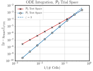
(a) Convergence of MDG-ICE($\mathcal{P}_{2}$) discretizations using the sub-optimal, $\mathcal{P}_{2}\left(\mathcal{T}_{h}\right)\times\mathbb{R}^{\left|\mathcal{E}_{h,0}\right|+1}$, test space given by weak formulation (2.28) and the optimal, $\mathcal{P}_{1}\left(\mathcal{T}_{h}\right)\times\mathbb{R}^{\left|\mathcal{E}_{h,0}\right|+1}$, test space given by weak formulation (2.26).

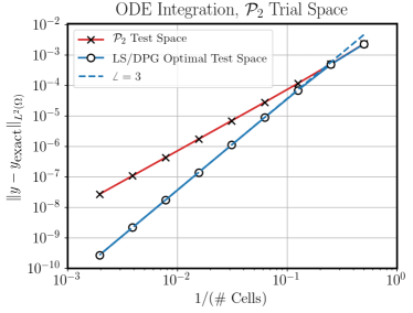
(b) Convergence of MDG-ICE($\mathcal{P}_{2}$) discretizations using the sub-optimal, $\mathcal{P}_{2}\left(\mathcal{T}_{h}\right)\times\mathbb{R}^{\left|\mathcal{E}_{h,0}\right|+1}$, test space given by weak formulation (2.28) and the optimal, $T\left(Y_{h}\right)$, test space given by weak formulation (2.27).

Figure 2.1: Convergence plots for solving an ODE integration problem with exact solution (2.29) using MDG-ICE($\mathcal{P}_{2}$) on a static grid with the sub-optimal, $\mathcal{P}_{2}\left(\mathcal{T}_{h}\right)\times\mathbb{R}^{\left|\mathcal{E}_{h,0}\right|+1}$, test space (2.28), the optimal, $\mathcal{P}_{1}\left(\mathcal{T}_{h}\right)\times\mathbb{R}^{\left|\mathcal{E}_{h,0}\right|+1}$, test space (2.26), and the automatically generated optimal test space (2.27). The coarsest grid consisted of $2$ line cells, while the finest grid consisted of $512$ line cells. Weak formulations (2.26) and (2.27) achieve optimal, third-order convergence, while the weak formulation (2.28) exhibits sub-optimal convergence behavior.

In order to verify both the optimality of weak formulations (2.22) and (2.25) and the sub-optimality of the weak formulation (2.24), we study their convergence under mesh refinement. Mesh refinement introduces a family of meshes $\mathcal{T}_{h}$ for which the set of interfaces $\mathcal{E}_{h}$ is increasingly dense as $h\rightarrow 0$. Ultra-weak DPG methods, which “break” the test space and introduce a mesh-dependent variational form cf. [6, 13], introduce interface unknowns on a mesh-dependent interface trial space over $\mathcal{E}_{h}$. In an analogous fashion, the DPG formulation of MDG-ICE, which “breaks” the trial space by defining $Y_{h}=\mathcal{P}_{p}\left(\mathcal{T}_{h}\right)$ and introduces a mesh-dependent variational form, enforces the interface condition on a mesh-dependent interface test space over $\mathcal{E}_{h}$. The mesh-dependent variational form is given as: find $y\in\mathcal{P}_{p}\left(\mathcal{T}_{h}\right)$ such that

$$b_{h}\left(y,\left(v,w\right)\right)=\sum_{\kappa\in\mathcal{T}_{h}}\left(y^{\prime},v\right)_{L^{2}\left(\kappa\right)}-y\left(0\right)w-\sum_{\epsilon\in\mathcal{E}_{h,0}}\left\llbracket y\right\rrbracket w=0\qquad\forall\left(v,w\right)\in\mathcal{P}_{p-1}\left(\mathcal{T}_{h}\right)\times\mathbb{R}^{\left|\mathcal{E}_{h,0}\right|+1}.$$ (2.26)

or, equivalently,

$$b_{h}\left(y,T_{h}\left(v\right)\right)=h\sum_{\kappa\in\mathcal{T}_{h}}\left(y^{\prime},v^{\prime}\right)_{L^{2}\left(\kappa\right)}-y\left(0\right)v\left(0\right)-\sum_{\epsilon\in\mathcal{E}_{h,0}}\left\llbracket y\right\rrbracket\left\llbracket v\right\rrbracket\qquad\forall v\in\mathcal{P}_{p}\left(\mathcal{T}_{h}\right).$$ (2.27)

As a result, the trial-to-test operator inherits a dependence on $\mathcal{T}_{h}$. Such a dependence also arises in the context of “practical” DPG methods where the inverse Riesz map defining the trial-to-test operator is approximated in a mesh-dependent fashion, the effect of which has been analyzed by Gopalakrishnan and Qiu [12]. We defer such analysis to future work and instead in the present study investigate the mesh or grid convergence behavior of solutions to  (2.26) and (2.27) as well as discrete least-squares solutions to: find $y\in\mathcal{P}_{p}\left(\mathcal{T}_{h}\right)$ such that

$$b_{h}\left(y,\left(v,w\right)\right)=\sum_{\kappa\in\mathcal{T}_{h}}\left(y^{\prime},v\right)_{L^{2}\left(\kappa\right)}-y\left(0\right)w-\sum_{\epsilon\in\mathcal{E}_{h,0}}\left\llbracket y\right\rrbracket w=0\qquad\forall\left(v,w\right)\in\mathcal{P}_{p}\left(\mathcal{T}_{h}\right)\times\mathbb{R}^{\left|\mathcal{E}_{h,0}\right|+1}.$$ (2.28)

We consider discrete trial spaces defined by $Y_{h}=\mathcal{P}_{2}\left(\mathcal{T}_{h}\right)$, and measure the $L^{2}$ error of these formulations with respect to an exact solution given by

$$y\left(x\right)=\left(x-0.1\right)\left(x-0.2\right)\left(x-0.3\right)\left(x-0.4\right)\left(x-0.5\right)\left(x-0.9\right)$$ (2.29)

generated by data $f=y^{\prime}$ and $y_{\text{in}}=y\left(0\right)$. Figure 2.1a shows that the formulation (2.26) defined using a $\mathcal{P}_{1}\left(\mathcal{T}_{h}\right)\times\mathbb{R}^{\left|\mathcal{E}_{h,0}\right|+1}$ test space achieves optimal, third-order convergence. Likewise, Figure 2.1b shows that the equivalent formulation (2.27) defined using the trial-to-test operator also achieves optimal, third-order convergence. We also observe the sub-optimal convergence behavior of the formulation (2.28) using an equal-order test space $\mathcal{P}_{2}\left(\mathcal{T}_{h}\right)\times\mathbb{R}^{\left|\mathcal{E}_{h,0}\right|+1}$. Having verified optimal-order convergence, in the following section, we proceed to extend LS-MDG-ICE from formulation (2.27) to a general setting.

3 Least-Squares Moving Discontinuous Galerkin Method with Interface Condition Enforcement

In this section, we derive the least-squares formulation of MDG-ICE for conservation laws governed by convection-diffusion with state independent source term data in arbitrary spatial dimensions. Let $\Omega\subset\mathbb{R}^{d}$ be a given domain. Our earlier work also considered unsteady problems where the domain is defined over space-time $\Omega\subset\mathbb{R}^{d=d_{x}+1}$, cf. [2, 3]. Although LS-MDG-ICE readily applies to unsteady problems, in the present work, we focus on steady problems defined over a spatial domain $\Omega\subset\mathbb{R}^{d=d_{x}}$. Throughout this work, we assume that $\Omega$ is partitioned by $\mathcal{T}$, consisting of disjoint sub-domains or cells $\kappa$, so that $\overline{\Omega}=\cup_{\kappa\in\mathcal{T}}\overline{\kappa}$, with interfaces $\epsilon$, composing a set $\mathcal{E}$ so that $\cup_{\epsilon\in\mathcal{E}}\epsilon=\cup_{\kappa\in\mathcal{T}}\partial\kappa$. Furthermore, we assume that each interface $\epsilon$ is oriented so that a unit normal $n:\epsilon\rightarrow\mathbb{R}^{d}$ is defined. For consistency of notation with earlier work [3], we also define the spatial normal $n_{x}:\epsilon\rightarrow\mathbb{R}^{d_{x}}$, which coincides with the normal $n$ in the spatial setting.

In Section 3.1 we present the governing equations. Then, in Section 3.2 we derive a least-squares formulation of MDG-ICE for both inviscid and viscous flows in physical space with static, discrete geometry. The most powerful aspect of MDG-ICE is its ability to fit a priori unknown interfaces and resolve otherwise under-resolved flow features. Therefore, in Section 3.3 we transform to reference space and introduce the discrete geometry as a variable, so that using DPG we systematically generate optimal test functions for the case of moving grid geometry.

3.1 Governing equations [3, Section 2.1]

In this work, we will apply LS-MDG-ICE to governing equations also considered in our earlier work [3], cf. Section 2.1. Consider a nonlinear conservation law governing the behavior of smooth, $\mathbb{R}^{m}$-valued, functions $y$,

$$\nabla\cdot\mathcal{F}\left(y,\nabla_{x}y\right)-\mathcal{S}\left(y\right)=0 \textup{ in }\Omega,$$ (3.1)

in terms of a given flux function, $\mathcal{F}:\mathbb{R}^{m}\times\mathbb{R}^{m\times d_{x}}\rightarrow\mathbb{R}^{m\times d}$ that depends on the flow state variable $y$ and its $d_{x}$-dimensional spatial gradient,

$$\nabla_{x}y=\left(\frac{\partial y}{\partial x_{1}},\ldots,\frac{\partial y}{\partial x_{d_{x}}}\right).$$ (3.2)

For unsteady flows, $\mathcal{F}$ is defined to be the space-time flux with $d=d_{x}+1$, cf. [3]. In the present work, we focus on the case of steady flows, $d=d_{x}$, so that $\mathcal{F}$ coincides with a given spatial flux, $\mathcal{F}^{x}:\mathbb{R}^{m}\times\mathbb{R}^{m\times d_{x}}\rightarrow\mathbb{R}^{m\times d_{x}}$. The spatial flux is defined in terms of a convective flux, which depends on the state variable only, and a viscous, or diffusive flux, which also depends on the spatial gradient of the state variable,

$$\mathcal{F}^{x}\left(y,\nabla_{x}y\right)=\mathcal{F}^{c}\left(y\right)-\mathcal{F}^{v}\left(y,\nabla_{x}y\right).$$ (3.3)

The governing equation (3.1) also incorporates a source term $\mathcal{S}:\mathbb{R}^{m}\rightarrow\mathbb{R}^{m}$, which in previous work we assumed to be zero [2, 3]. Here, we incorporate a source term of the form $\mathcal{S}\left(y\right)=f$, defined in terms of data $f\in\mathbb{R}^{m}$ that is independent of both the state $y$ and position $x\in\Omega$.

3.1.1 Linear advection-diffusion

Linear advection-diffusion involves a single-component flow state variable $y:\Omega\rightarrow\mathbb{R}^{1}$ with a linear diffusive flux,

$$\mathcal{F}^{v}\left(y,\nabla_{x}y\right)=\epsilon\nabla_{x}y,$$ (3.4)

that is independent of the state $y$, where the coefficient $\epsilon$ represents mass diffusivity. The convective flux is given as

$$\mathcal{F}^{c}\left(y\right)=\left(v_{1}y,\ldots,v_{d_{x}}y\right),$$ (3.5)

where $\left(v_{1},\ldots,v_{d_{x}}\right)\in\mathbb{R}^{d_{x}}$ is a prescribed spatial velocity that in the present setting is assumed to be uniform.

3.1.2 One-dimensional Burgers flow

As in the case of linear advection-diffusion, one-dimensional Burgers flow involves a single-component flow state variable $y:\Omega\rightarrow\mathbb{R}^{1}$ with a linear viscous flux,

$$\mathcal{F}^{v}\left(y,\nabla y\right)=\epsilon\nabla y,$$ (3.6)

is independent of the state $y$, where the coefficient $\epsilon$ represents viscosity. The convective flux is given as

$$\mathcal{F}^{c}\left(y\right)=\left(\frac{1}{2}y^{2}\right).$$ (3.7)

3.1.3 Compressible Navier-Stokes flow

For compressible Navier-Stokes flow, the state variable $y:\Omega\rightarrow\mathbb{R}^{m}$, where $m=d_{x}+2$, is given by

$$y=\left(\rho,\rho v_{1},\ldots,\rho v_{d_{x}},\rho E\right).$$ (3.8)

The $i$-th spatial component of the convective flux, $\mathcal{F}^{c}:\mathbb{R}^{m}\rightarrow\mathbb{R}^{m\times d_{x}}$, is

$$\mathcal{F}_{i}^{c}\left(y\right)=\left(\rho v_{i},\rho v_{i}v_{1}+p\delta_{i1},\ldots,\rho v_{i}v_{d_{x}}+p\delta_{id_{x}},\rho Hv_{i}\right),$$ (3.9)

where $\delta_{ij}$ is the Kronecker delta, $\rho:\Omega\rightarrow\mathbb{R}_{+}$ is density, $\left(v_{1},\ldots,v_{d_{x}}\right):\mathbb{R}^{m}\rightarrow\mathbb{R}^{d_{x}}$ is velocity, $\rho E:\Omega\rightarrow\mathbb{R}_{+}$ is stagnation energy per unit volume, and

$$H=\left(\rho E+p\right)/\rho$$ (3.10)

is stagnation enthalpy, where $H:\mathbb{R}^{m}\rightarrow\mathbb{R}_{+}$. Assuming that the fluid is a perfect gas, the pressure $p:\mathbb{R}^{m}\rightarrow\mathbb{R}_{+}$ is defined as

$$p=\left(\gamma-1\right)\left(\rho E-\frac{1}{2}\sum_{i=1}^{d_{x}}\rho v_{i}v_{i}\right),$$ (3.11)

where the ratio of specific heats for air is given as $\gamma=1.4$. The $i$-th spatial component of the viscous flux is given by

$$\mathcal{F}_{i}^{\nu}\left(y,\nabla y\right)=\left(0,\tau_{1i},\ldots,\tau_{d_{x}i},\sum_{j=1}^{d_{x}}\tau_{ij}v_{j}-q_{i}\right),$$ (3.12)

where $q:\mathbb{R}^{m}\times\mathbb{R}^{m\times d_{x}}\rightarrow\mathbb{R}^{d_{x}}$ is the thermal heat flux, $\tau:\mathbb{R}^{m}\times\mathbb{R}^{m\times d_{x}}\rightarrow\mathbb{R}^{d_{x}\times d_{x}}$ is the viscous stress tensor. The $i$-th spatial component of the thermal heat flux is given by

$$q_{i}=-k\frac{\partial T}{\partial x_{i}},$$ (3.13)

where $T:\mathbb{R}^{m}\rightarrow\mathbb{R}_{+}$ is the temperature and $k$ is thermal conductivity. The temperature $T$ is defined as

$$T=\frac{p}{R\rho},$$ (3.14)

where $R=287$ is the mixed specific gas constant for air. The $i$-th spatial component of the viscous stress tensor is given by

$$\tau_{i}=\mu\left(\frac{\partial v_{1}}{\partial x_{i}}+\frac{\partial v_{i}}{\partial x_{1}}-\delta_{i1}\frac{2}{3}\sum_{j=1}^{d_{x}}\frac{\partial v_{j}}{\partial x_{j}},\ldots,\frac{\partial v_{d_{x}}}{\partial x_{i}}+\frac{\partial v_{i}}{\partial x_{d_{x}}}-\delta_{id_{x}}\frac{2}{3}\sum_{j=1}^{d_{x}}\frac{\partial v_{j}}{\partial x_{j}}\right),$$ (3.15)

where $\mu$ is the dynamic viscosity coefficient.

3.2 Formulation in physical space with fixed geometry

We consider the first-order system corresponding to convection-diffusion that includes a conservation law, constitutive law, and the corresponding interface conditions. The viscous interface conditions, more specifically the viscous contribution to (3.18) and (3.19), were derived in Section 2.2 of our earlier work [3].

3.2.1 Strong formulation [3, Section 2.3.1]

We consider the strong formulation presented in Section 2.3.1 of our earlier work [3] involving a nonlinear conservation law, generalized constitutive law, and their corresponding interface conditions,

$$\nabla\cdot\mathcal{F}\left(y,\sigma\right)-f=0 \textup{ in }\kappa\qquad\forall\kappa\in\mathcal{T},$$ (3.16)

$$\sigma-G(y)\nabla_{x}y=0 \textup{ in }\kappa\qquad\forall\kappa\in\mathcal{T},$$ (3.17)

$$\left\llbracket n\cdot\mathcal{F}\left(y,\sigma\right)\right\rrbracket=0 \textup{ on }\epsilon\qquad\forall\epsilon\in\mathcal{E},$$ (3.18)

$$\left\{\!\!\left\{G\left(y\right)\right\}\!\!\right\}\left\llbracket y\otimes n_{x}\right\rrbracket=0 \textup{ on }\epsilon\qquad\forall\epsilon\in\mathcal{E},$$ (3.19)

governing the flow state variable $y$ and auxiliary variable $\sigma$. The interface condition (3.18) corresponding to the conservation law (3.16) is the jump or Rankine-Hugoniot condition [48], which accounts for both the convective and viscous flux, ensuring continuity of the normal flux at the interface. The interface condition (3.19) corresponds to the constitutive law (3.17) and enforces a constraint on the continuity of the state variable at the interface.

The flux $\mathcal{F}\left(y,\sigma\right)$ is now defined

$$\mathcal{F}\left(y,\sigma\right)=\mathcal{F}^{c}\left(y\right)-\mathcal{\tilde{F}}^{v}\left(y,\sigma\right),$$ (3.20)

in terms of the convective flux and a modified viscous flux $\tilde{F}^{v}:\mathbb{R}^{m}\times\mathbb{R}^{m\times d_{x}}\rightarrow\mathbb{R}^{m\times d_{x}}$ . The modified viscous flux is defined consistently with the primal formulation of Section 3.1, as

$$\mathcal{F}^{v}\left(y,\nabla_{x}y\right)=\mathcal{\tilde{F}}^{v}\left(y,G\left(y\right)\nabla_{x}y\right),$$ (3.21)

where $G\left(y\right)\in\mathbb{R}^{m\times d_{x}\times m\times d_{x}}$ is a generalized constitutive tensor that depends on the specific choice of constitutive law, a detailed discussion of which is provided in our earlier work [3]. In this work, we continue to use the flux formulation [3] in the case of linear advection-diffusion and viscous Burgers flow, where the constitutive tensor is defined so that

$$G\left(y\right)\nabla_{x}y=\mathcal{F}^{v}\left(y,\nabla_{x}y\right)=\mathcal{F}_{\nabla_{x}y}^{v}\left(y,\nabla_{x}y\right)\nabla_{x}y,$$ (3.22)

and the modified viscous flux is defined to be the auxiliary variable,

$$\mathcal{\tilde{F}}^{v}\left(y,\sigma\right)=\sigma.$$ (3.23)

In the case of compressible Navier-Stokes flow, we define $G\left(y\right)\nabla_{x}y$, up to a factor $\mu_{\infty}^{-\nicefrac{{1}}{{2}}}$, as the viscous stress tensor, $\tau$, given by (3.15) and thermal heat flux, $q$, given by (3.13)., which is an approach similar to that of Chan et al. [18] while also incorporating the scaling advocated by Broersen and Stevenson [49, 50] and later Demkowicz and Gopalakrishnan [9]. Thus, the constitutive tensor $G\left(y\right)$ is defined such that

$$\left(G\left(y\right)\nabla y\right)_{i}=\mu_{\infty}^{-\nicefrac{{1}}{{2}}}\left(0,\tau_{1i},\ldots,\tau_{d_{x}i},-q_{i}\right),$$ (3.24)

where $\mu_{\infty}$ is the freestream dynamic viscosity and the viscous flux is defined in terms of the auxiliary variable as

$$\mathcal{F}_{i}^{v}\left(y,\sigma\right)=\mu_{\infty}^{\nicefrac{{1}}{{2}}}\left(\sigma_{1i},\sigma_{2i},\ldots,\sigma_{d_{x}+1i},\sigma_{i+1j}v_{j}+\sigma_{mi}\right).$$ (3.25)

3.2.2 Interior and boundary interfaces [3, Section 2.3.2]

We assume that $\mathcal{E}$ consists of two disjoint subsets: the interior interfaces $\mathcal{E}_{0}=\left\{\epsilon_{0}\in\mathcal{E}\,\middle|\,\epsilon_{0}\cap\partial\Omega=\emptyset\right\}$ and exterior interfaces $\mathcal{E}_{\partial}=\left\{\epsilon_{\partial}\in\mathcal{E}\,\middle|\,\epsilon_{\partial}\subset\partial\Omega\right\},$ so that $\mathcal{E}=\mathcal{E}_{0}\cup\mathcal{E}_{\partial}$. For interior interfaces $\epsilon_{0}\in\mathcal{E}_{0}$ there exists $\kappa^{+},\kappa^{-}\in\mathcal{T}$ such that $\epsilon_{0}=\partial\kappa^{+}\cap\partial\kappa^{-}$. On interior interfaces Equations (3.18), (3.19) are defined as

$$\left\llbracket n\cdot\mathcal{F}\left(y,\sigma\right)\right\rrbracket=n^{+}\cdot\mathcal{F}\left(y^{+},\sigma^{+}\right)+n^{-}\cdot\mathcal{F}\left(y^{-},\sigma^{-}\right)=0, \textup{ on }\epsilon\qquad\forall\epsilon\in\mathcal{E}_{0},$$ (3.26)

$$\left\{\!\!\left\{G\left(y\right)\right\}\!\!\right\}\left\llbracket y\otimes n_{x}\right\rrbracket=\frac{1}{2}\left(G\left(y^{+}\right)+G\left(y^{-}\right)\right)\left(y^{+}\otimes n_{x}^{+}+y^{-}\otimes n_{x}^{-}\right)=0, \textup{ on }\epsilon\qquad\forall\epsilon\in\mathcal{E}_{0}.$$ (3.27)

where $n^{+},n^{-}$ denote the outward facing normal of $\kappa^{+},\kappa^{-}$ respectively, so that $n^{+}=-n^{-}$. For exterior interfaces

$$\left\llbracket n\cdot\mathcal{F}\left(y,\sigma\right)\right\rrbracket=n^{+}\cdot\mathcal{F}\left(y^{+},\sigma^{+}\right)-n^{+}\cdot\mathcal{\mathcal{F}}_{\partial}\left(y^{+},\sigma^{+}\right)=0, \textup{ on }\epsilon\qquad\forall\epsilon\in\mathcal{E}_{\partial},$$ (3.28)

$$\left\{\!\!\left\{G\left(y\right)\right\}\!\!\right\}\left\llbracket y\otimes n_{x}\right\rrbracket=G_{\partial}\left(y^{+}\right)\left(y^{+}\otimes n_{x}^{+}-y_{\partial}\left(y^{+}\right)\otimes n_{x}^{+}\right)=0, \textup{ on }\epsilon\qquad\forall\epsilon\in\mathcal{E}_{\partial}.$$ (3.29)

Here $n^{+}\cdot\mathcal{F}_{\partial}\left(y^{+},\sigma^{+}\right)$ is the imposed normal boundary flux, $G_{\partial}\left(y^{+}\right)$ is the boundary modified homogeneity tensor, and $y_{\partial}\left(y^{+}\right)$ is the boundary state, which are functions chosen depending on the type of boundary condition. Therefore, we further decompose $\mathcal{E}_{\partial}$ into disjoint subsets of inflow and outflow interfaces $\mathcal{E}_{\partial}=\mathcal{E}_{\text{in}}\cup\mathcal{E}_{\text{out}},$ so that at an outflow interface $\epsilon_{\textup{out}}$ the boundary flux is defined as the interior convective flux, and the boundary state is defined as the interior state,

$$n^{+}\cdot\mathcal{F}_{\partial}\left(y^{+},\sigma^{+}\right)=n^{+}\cdot\mathcal{F}\left(y^{+},\sigma_{\text{out}}=0\right), \textup{ on }\epsilon\qquad\forall\epsilon\in\mathcal{E}_{\text{out}},$$ (3.30)

$$G_{\partial}\left(y^{+}\right)=G\left(y^{+}\right), \textup{ on }\epsilon\qquad\forall\epsilon\in\mathcal{E}_{\text{out}},$$ (3.31)

$$y_{\partial}\left(y^{+}\right)=y^{+}, \textup{ on }\epsilon\qquad\forall\epsilon\in\mathcal{E}_{\text{out}},$$ (3.32)

and therefore (3.29) is satisfied trivially. At an inflow boundary $\epsilon_{\textup{in}}\in\mathcal{E}_{\text{in}}$, the normal convective boundary flux and boundary state are prescribed values independent of the interior state $y^{+}$ , while the normal viscous boundary flux is defined as the interior normal viscous flux,

$$n^{+}\cdot\mathcal{\mathcal{F}}_{\partial}\left(y^{+},\sigma^{+}\right)=n^{+}\cdot\mathcal{\mathcal{F}}_{\text{in}}^{c}-n^{+}\cdot\mathcal{\tilde{F}}^{v}\left(y_{\partial}\left(y^{+}\right),\sigma^{+}\right), \textup{ on }\epsilon\qquad\forall\epsilon\in\mathcal{E}_{\text{in}},$$ (3.33)

$$G_{\partial}\left(y^{+}\right)=G\left(y_{\partial}\left(y^{+}\right)\right), \textup{ on }\epsilon\qquad\forall\epsilon\in\mathcal{E}_{\text{in}},$$ (3.34)

$$y_{\partial}\left(y^{+}\right)=y_{\text{in}}, \textup{ on }\epsilon\qquad\forall\epsilon\in\mathcal{E}_{\text{in}}.$$ (3.35)

3.2.3 Least-squares weak formulation

We now describe a least-squares weak formulation of MDG-ICE in physical space. Before proceeding, we note that special care is required to weight the interface condition terms in the weak formulation in physical space. If $h$ represents an element length scale, then a scaling $h^{-1}$ arises in an inverse inequality that applies to functions $v$ in a finite-dimensional subspace $V_{h}$,

$$\left(v,v\right)_{H^{1/2}\left(\epsilon\right)}=\left\|v\right\|_{H^{1/2}\left(\epsilon\right)}^{2}\leq Ch^{-1}\left\|v\right\|_{L^{2}\left(\epsilon\right)}^{2},$$ (3.36)

where $C$ is a positive constant independent of $h$, cf. the works of Bochev and Gunzberger [15, (4.22)–(4.23)], Cao and Gunzburger [23, (3.6)], and Guermond [51, (3.3)]. Practically speaking, the element integrals that arise in LS-MDG-ICE over $\kappa$ scale proportionally to $h^{d-2}$ while the interface integrals over $\epsilon$ scale proportionally to $h^{d-1}$. This scaling has been accounted for in other least-squares finite element methods involving interface or jump condition enforcement, cf. the works of Cao and Gunzburger [23] and Gerritsma and Proot [22]. We present an LS-MDG-ICE formulation in physical space in order to illustrate the methodology that will be used to derive the reference space formulation, and to this end, we neglect the scaling. However, the scaling will be naturally accounted for in the process of transforming to a reference space least-squares formulation in Section 3.3. Therefore, the results presented in Section 4 will use the reference space formulation of Section 3.3 even in the case of a static grid.

The solution spaces $Y$ and $\Sigma$ are the broken Sobolev spaces,

$$Y = \left\{y\in\left[L^{2}\left(\Omega\right)\right]^{m\hphantom{\times d_{x}}}\bigl{|}\forall\kappa\in\mathcal{T},\>\>\hphantom{\nabla_{x}\cdot}\left.y\right|_{\kappa}\in\left[H^{1}\left(\kappa\right)\right]^{m}\right\},$$ (3.37)

$$\Sigma = \left\{\sigma\in\left[L^{2}\left(\Omega\right)\right]^{m\times d_{x}}\bigl{|}\forall\kappa\in\mathcal{T},\left.\nabla_{x}\cdot\sigma\right|_{\kappa}\in\left[\>L^{2}\left(\kappa\right)\right]^{m}\right\},$$ (3.38)

defined over a mesh $\mathcal{T}$. The test spaces are defined as $V_{y}=\left[L^{2}\left(\Omega\right)\right]^{m}$ and $V_{\sigma}=\left[L^{2}\left(\Omega\right)\right]^{m\times d_{x}}$, with $W_{y}$ and $W_{\sigma}$ defined to be the corresponding single-valued trace spaces, cf. Carstensen et al. [13]. We integrate (3.16)-(3.19) on each element and interface against separate test functions to define a nonlinear state operator,

$$e:Y\times\Sigma\rightarrow\left(V_{y}\times V_{\sigma}\times W_{y}\times W_{\sigma}\right)^{*}$$ (3.39)

where,

$$\left\langle e\left(y,\sigma\right),\left(v,\tau,w_{y},w_{\sigma}\right)\right\rangle= \;\;\;\;\sum_{\kappa\in\mathcal{T}}\left(\nabla\cdot\mathcal{F}\left(y,\sigma\right)-f,v\right)_{\kappa}$$

$$+\sum_{\kappa\in\mathcal{T}}\left(\sigma-G(y)\nabla_{x}y,\tau\right)_{\kappa}$$

$$-\sum_{\epsilon\in\mathcal{E}}\left(\left\llbracket n\cdot\mathcal{F}\left(y,\sigma\right)\right\rrbracket,w_{y}\right)_{\epsilon}$$

$$-\sum_{\epsilon\in\mathcal{E}}\left(\left\{\!\!\left\{G\left(y\right)\right\}\!\!\right\}\left\llbracket y\otimes n_{x}\right\rrbracket,w_{\sigma}\right)_{\epsilon},$$ (3.40)

for $\left(y,\sigma\right)\in Y\times\Sigma$ and $\left(v,\tau,w_{y},w_{\sigma}\right)\in V_{y}\times V_{\sigma}\times W_{y}\times W_{\sigma}$. Due to the nonlinear state operator, the trial-to-test operator is defined in terms of the linearization of the state operator, cf. [18, 52]. Given $\left(y,\sigma\right)\in Y\times\Sigma$, we have

$$T\left(y,\sigma\right):Y\times\Sigma\rightarrow V_{y}\times V_{\sigma}\times W_{y}\times W_{\sigma},$$ (3.41)

defined for $\left(v_{y},v_{\sigma}\right)\in Y\times\Sigma$ by

$$T\left(y,\sigma\right)=\left(v_{y},v_{\sigma}\right)\mapsto R_{V}^{-1}e^{\prime}\left(y,\sigma\right)\left(v_{y},v_{\sigma}\right),$$ (3.42)

where make use of Riesz map notation, cf. [6],

$$R_{V}=R_{V_{y}\times V_{\sigma}\times W_{y}\times W_{\sigma}}:\left(V_{y}\times V_{\sigma}\times W_{y}\times W_{\sigma}\right)\rightarrow\left(V_{y}\times V_{\sigma}\times W_{y}\times W_{\sigma}\right)^{*}.$$ (3.43)

Since each test space is equipped with an $L^{2}$ inner product, we can write the trial-to-test-operator as

$$T\left(y,\sigma\right):\left(v_{y},v_{\sigma}\right)\mapsto\left(v^{\text{opt}},\tau^{\text{opt}},w_{y}^{\text{opt}},w_{\sigma}^{\text{opt}}\right),$$ (3.44)

with

$$v^{\text{opt}}= \nabla\cdot\left(\mathcal{F}^{\prime}\left(y,\sigma\right)\left(v_{y},v_{\sigma}\right)\right),$$

$$\tau^{\text{opt}}= v_{\sigma}-\left(\left(G^{\prime}\left(y\right)v_{y}\right)\nabla_{x}y+G\left(y\right)\nabla_{x}v_{y}\right),$$

$$w_{y}^{\text{opt}}= \left\llbracket n\cdot\left(\mathcal{F}^{\prime}\left(y,\sigma\right)\left(v_{y},v_{\sigma}\right)\right)\right\rrbracket,$$

$$w_{\sigma}^{\text{opt}}= \left\{\!\!\left\{G^{\prime}\left(y\right)v_{y}\right\}\!\!\right\}\left\llbracket y\otimes n_{x}\right\rrbracket+\left\{\!\!\left\{G\left(y\right)\right\}\!\!\right\}\left\llbracket v_{y}\otimes n_{x}\right\rrbracket.$$ (3.45)

Therefore, the DPG/least-squares formulation is given as: find $\left(y,\sigma\right)\in Y\times\Sigma$ such that

$$0= \;\;\;\;\sum_{\kappa\in\mathcal{T}}\left(\nabla\cdot\mathcal{F}\left(y,\sigma\right)-f,v^{\text{opt}}\right)_{\kappa}$$

$$+\sum_{\kappa\in\mathcal{T}}\left(\sigma-\left(G\left(y\right)\nabla_{x}y\right),\tau^{\text{opt}}\right)_{\kappa}$$

$$-\sum_{\epsilon\in\mathcal{E}}\left(\left\llbracket n\cdot\mathcal{F}\left(y,\sigma\right)\right\rrbracket,w_{y}^{\text{opt}}\right)_{\epsilon}$$

$$-\sum_{\epsilon\in\mathcal{E}}\left(\left\{\!\!\left\{G\left(y\right)\right\}\!\!\right\}\left\llbracket y\otimes n_{x}\right\rrbracket,w_{\sigma}^{\text{opt}}\right)_{\epsilon}\qquad\forall\left(v_{y},v_{\sigma}\right)\in Y\times\Sigma,$$ (3.46)

or abstractly as: find $\left(y,\sigma\right)\in Y\times\Sigma$ such that

$$\left\langle e\left(y,\sigma\right),R_{V}^{-1}\left(e^{\prime}\left(y,\sigma\right)\left(v_{y},v_{\sigma}\right)\right)\right\rangle=0\qquad\forall\left(v_{y},v_{\sigma}\right)\in Y\times\Sigma.$$ (3.47)

where we note that the scaling (3.36) is not yet accounted for.

3.3 Formulation in reference space with variable geometry

In this section, we transform the strong and weak formulation to reference space, leading to a DPG/least-squares formulation of MDG-ICE, while introducing the grid as a variable in order to fit interfaces and resolve initially under-resolved solution features. We assume that there is a continuous, invertible mapping

$$u:\hat{\Omega}\rightarrow\Omega,$$ (3.48)

from a reference domain $\hat{\Omega}\subset\mathbb{R}^{d}$ to the physical domain $\Omega\subset\mathbb{R}^{d}$. We assume that $\hat{\Omega}$ is partitioned by $\hat{\mathcal{T}}$, so that $\overline{\hat{\Omega}}=\cup_{\hat{\kappa}\in\hat{\mathcal{T}}}\overline{\hat{\kappa}}$. Also, we consider the set of interfaces $\hat{\mathcal{E}}$ consisting of disjoint interfaces $\hat{\epsilon}$, such that $\cup_{\hat{\epsilon}\in\hat{\mathcal{E}}}\hat{\epsilon}=\cup_{\hat{\kappa}\in\hat{\mathcal{T}}}\partial\hat{\kappa}$. The strong form in reference space [3] is

$$\left(\operatorname{cof}\left(\nabla u\right)\nabla\right)\cdot\mathcal{F}\left(y,\sigma\right)-\operatorname{det}\left(\nabla u\right)f=0 \textup{ in }\hat{\kappa}\qquad\forall\hat{\kappa}\in\hat{\mathcal{T}},$$ (3.49)

$$\operatorname{det}\left(\nabla u\right)\sigma-G(y)\left(\operatorname{cof}\left(\nabla u\right)\nabla\right)_{x}y=0 \textup{ in }\hat{\kappa}\qquad\forall\hat{\kappa}\in\hat{\mathcal{T}},$$ (3.50)

$$\left\llbracket s\left(\nabla u\right)\cdot\mathcal{F}\left(y,\sigma\right)\right\rrbracket=0 \textup{ on }\hat{\epsilon}\qquad\forall\hat{\epsilon}\in\hat{\mathcal{E}},$$ (3.51)

$$\left\{\!\!\left\{G\left(y\right)\right\}\!\!\right\}\left\llbracket y\otimes s\left(\nabla u\right)_{x}\right\rrbracket=0 \textup{ on }\hat{\epsilon}\qquad\forall\hat{\epsilon}\in\hat{\mathcal{E}},$$ (3.52)

$$b\left(u\right)-u=0 \textup{ on }\hat{\epsilon}\qquad\forall\hat{\epsilon}\in\hat{\mathcal{E}}.$$ (3.53)

where $\nabla u$ is the Jacobian of the mapping from reference to physical space, $\operatorname{det}\left(\nabla u\right)$ is the determinant of the Jacobian, and $\operatorname{cof}\left(\nabla u\right)=\operatorname{det}\left(\nabla u\right)\left(\nabla u\right)^{-\top}$ is the cofactor matrix. The scaled normal $s\left(\nabla u\right)$ is the physical space normal scaled by the magnitude of generalized cross product of the tangent plane basis vectors of a parameterization of the physical space interface, as detailed in previous work [2, 3]. On elements $\kappa$ and interfaces $\epsilon$ with length scale $h$, $\left(\operatorname{cof}\left(\nabla u\right)\nabla\right)$ and $s\left(\nabla u\right)$ both scale proportionally to $h^{d-1}$ accounting for the scaling discussed in Section 3.2.3. In a spatial setting, $\left(\operatorname{cof}\left(\nabla u\right)\nabla\right)_{x}=\left(\operatorname{cof}\left(\nabla u\right)\nabla\right)$ and $s\left(\nabla u\right)_{x}=s\left(\nabla u\right)$. Equation (3.53) constrains points to the boundary of the physical domain via a projection operator $b:U\rightarrow U$, where the space of mappings from reference space to physical space, $U=\left[H^{1}\left(\hat{\Omega}\right)\right]^{d},$ is the $\mathbb{R}^{d}$-valued Sobolev space over $\hat{\Omega}$, cf. the previous work [2, 3]. We assume that $Y$ and $\Sigma$ now consist of functions defined in $\mathbb{R}^{m}$-valued and $\mathbb{R}^{m\times d_{x}}$-valued broken Sobolev spaces over $\hat{\mathcal{T}}$ respectively. We further assume that the test spaces $V_{y}=\left[L^{2}\left(\hat{\Omega}\right)\right]^{m}$ and $V_{\sigma}=\left[L^{2}\left(\hat{\Omega}\right)\right]^{m\times d_{x}}$, along with the single-valued trace test spaces, $W_{y}$ and $W_{\sigma}$, now consist of functions defined over reference space.

As in our previous work [3], we define a provisional state operator $\tilde{e}:Y\times\Sigma\times U\rightarrow\left(V_{y}\times V_{\sigma}\times W_{y}\times W_{\sigma}\right)^{*}$ for $\left(y,\sigma,u\right)\in Y\times\Sigma\times U$, by

$$\tilde{e}\left(y,\sigma,u\right)=\left(v,\tau,w_{y},w_{\sigma}\right)\mapsto \;\;\;\;\sum_{\hat{\kappa}\in\hat{\mathcal{T}}}\left(\left(\operatorname{cof}\left(\nabla u\right)\nabla\right)\cdot\mathcal{F}\left(y,\sigma\right)-\operatorname{det}\left(\nabla u\right)f,v\right)_{\hat{\kappa}}$$

$$+\sum_{\hat{\kappa}\in\hat{\mathcal{T}}}\left(\operatorname{det}\left(\nabla u\right)\sigma-G(y)\left(\operatorname{cof}\left(\nabla u\right)\nabla\right)_{x}y,\tau\right)_{\hat{\kappa}}$$

$$-\sum_{\hat{\epsilon}\in\hat{\mathcal{E}}}\left(\left\llbracket s\left(\nabla u\right)\cdot\mathcal{F}\left(y,\sigma\right)\right\rrbracket,w_{y}\right)_{\hat{\epsilon}}$$

$$-\sum_{\hat{\epsilon}\in\hat{\mathcal{E}}}\left(\left\{\!\!\left\{G\left(y\right)\right\}\!\!\right\}\left\llbracket y\otimes s\left(\nabla u\right)_{x}\right\rrbracket,w_{\sigma}\right)_{\hat{\epsilon}}$$ (3.54)

which has a Fréchet derivative defined for perturbation $\left(\delta y,\delta\sigma,\delta u\right)\in Y\times\Sigma\times U$, and test functions $\left(v,\tau,w_{y},w_{\sigma}\right)\in V_{y}\times V_{\sigma}\times W_{y}\times W_{\sigma}$, by its partial derivative with respect to the state variable $y$,

$$\tilde{e}_{y}\left(y,\sigma,u\right)\delta y=\left(v,\tau,w_{y},w_{\sigma}\right)\mapsto \;\;\;\;\sum_{\hat{\kappa}\in\hat{\mathcal{T}}}\left(\left(\operatorname{cof}\left(\nabla u\right)\nabla\right)\cdot\left(\mathcal{F}_{y}\left(y,\sigma\right)\delta y\right),v\right)_{\hat{\kappa}}$$

$$-\sum_{\hat{\kappa}\in\hat{\mathcal{T}}}\left(\left(G^{\prime}(y)\delta y\right)\left(\operatorname{cof}\left(\nabla u\right)\nabla\right)_{x}y+G(y)\left(\operatorname{cof}\left(\nabla u\right)\nabla\right)_{x}\delta y,\tau\right)_{\hat{\kappa}}$$

$$-\sum_{\hat{\epsilon}\in\hat{\mathcal{E}}}\left(\left\llbracket s\left(\nabla u\right)\cdot\left(\mathcal{F}_{y}\left(y,\sigma\right)\delta y\right)\right\rrbracket,w_{y}\right)_{\hat{\epsilon}}$$

$$-\sum_{\hat{\epsilon}\in\hat{\mathcal{E}}}\left(\left\{\!\!\left\{G^{\prime}\left(y\right)\delta y\right\}\!\!\right\}\left\llbracket y\otimes s\left(\nabla u\right)_{x}\right\rrbracket+\left\{\!\!\left\{G\left(y\right)\right\}\!\!\right\}\left\llbracket\delta y\otimes s\left(\nabla u\right)_{x}\right\rrbracket,w_{\sigma}\right)_{\hat{\epsilon}},$$ (3.55)

its partial derivative with respect to the auxiliary variable $\sigma$,

$$\tilde{e}_{\sigma}\left(y,\sigma,u\right)\delta\sigma=\left(v,\tau,w_{y},w_{\sigma}\right)\mapsto \;\;\;\;\sum_{\hat{\kappa}\in\hat{\mathcal{T}}}\left(\left(\operatorname{cof}\left(\nabla u\right)\nabla\right)\cdot\left(\mathcal{F}_{\sigma}\left(y,\sigma\right)\delta\sigma\right),v\right)_{\hat{\kappa}}$$

$$+\sum_{\hat{\kappa}\in\hat{\mathcal{T}}}\left(\operatorname{det}\left(\nabla u\right)\delta\sigma,\tau\right)_{\hat{\kappa}}$$

$$-\sum_{\hat{\epsilon}\in\hat{\mathcal{E}}}\left(\left\llbracket s\left(\nabla u\right)\cdot\left(\mathcal{F}_{\sigma}\left(y,\sigma\right)\delta\sigma\right)\right\rrbracket,w_{y}\right)_{\hat{\epsilon}},$$ (3.56)

and its partial derivative with respect to the geometry variable $u$,

$$\tilde{e}_{u}\left(y,\sigma,u\right)\delta u=\left(v,\tau,w_{y},w_{\sigma}\right)\mapsto \;\;\;\;\sum_{\hat{\kappa}\in\hat{\mathcal{T}}}\left(\left(\left(\operatorname{cof}^{\prime}\left(\nabla u\right)\nabla\delta u\right)\nabla\right)\cdot\mathcal{F}\left(y,\sigma\right)-\left(\operatorname{det}^{\prime}\left(\nabla u\right)\nabla\delta u\right)f,v\right)_{\hat{\kappa}}$$

$$+\sum_{\hat{\kappa}\in\hat{\mathcal{T}}}\left(\left(\operatorname{det}^{\prime}\left(\nabla u\right)\nabla\delta u\right)\sigma-G(y)\left(\left(\operatorname{cof}^{\prime}\left(\nabla u\right)\nabla\delta u\right)\nabla\right)_{x}y,\tau\right)_{\hat{\kappa}}$$

$$-\sum_{\hat{\epsilon}\in\mathcal{\hat{E}}}\left(\left\llbracket\left(s^{\prime}\left(\nabla u\right)\nabla\delta u\right)\cdot\mathcal{F}\left(y,\sigma\right)\right\rrbracket,w_{y}\right)_{\hat{\epsilon}}$$

$$-\sum_{\hat{\epsilon}\in\hat{\mathcal{E}}}\left(\left\{\!\!\left\{G\left(y\right)\right\}\!\!\right\}\left\llbracket y\otimes\left(s^{\prime}\left(\nabla u\right)\nabla\delta u\right)_{x}\right\rrbracket,w_{\sigma}\right)_{\hat{\epsilon}}.$$ (3.57)

In order to derive the LS-MDG-ICE formulation, we define the trial-to-test operator

$$T\left(y,\sigma,u\right):Y\times\Sigma\times U\rightarrow V_{y}\times V_{\sigma}\times W_{y}\times W_{\sigma},$$ (3.58)

for $\left(v_{y},v_{\sigma},v_{u}\right)\in Y\times\Sigma\times U$ by

$$T\left(y,\sigma,u\right)=\left(v_{y},v_{\sigma},v_{u}\right)\mapsto R_{V}^{-1}\left(\tilde{e}^{\prime}\left(y,\sigma,u\right)\left(v_{y},v_{\sigma},v_{u}\right)\right),$$ (3.59)

where we continue to employ the inverse Riesz map (3.43). Analogous to the physical space formulation, since each test space is equipped with an $L^{2}$ inner product, the trial-to-test operator can be expressed as

$$T:\left(v_{y},v_{\sigma},v_{u}\right)\mapsto\left(v^{\text{opt}},\tau^{\text{opt}},w_{y}^{\text{opt}},w_{\sigma}^{\text{opt}}\right),$$ (3.60)

where

$$v^{\text{opt}}= \left(\operatorname{cof}\left(\nabla u\right)\nabla\right)\cdot\left(\mathcal{F}^{\prime}\left(y,\sigma\right)\left(v_{y},v_{\sigma}\right)\right)$$

$$+\left(\left(\operatorname{cof}^{\prime}\left(\nabla u\right)\nabla v_{u}\right)\nabla\right)\cdot\mathcal{F}\left(y,\sigma\right)$$

$$-\left(\operatorname{det}^{\prime}\left(\nabla u\right)\nabla v_{u}\right)f,$$ (3.61)

$$\tau^{\text{opt}}= \operatorname{det}\left(\nabla u\right)v_{\sigma}+\left(\operatorname{det}^{\prime}\left(\nabla u\right)\nabla v_{u}\right)\sigma$$

$$-\left(G^{\prime}\left(y\right)v_{y}\right)\left(\operatorname{cof}\left(\nabla u\right)\nabla\right)_{x}y$$

$$-G\left(y\right)\left(\operatorname{cof}\left(\nabla u\right)\nabla\right)_{x}v_{y}$$

$$-G\left(y\right)\left(\left(\operatorname{cof}^{\prime}\left(\nabla u\right)\nabla v_{u}\right)\nabla\right)_{x}y,$$ (3.62)

$$w_{y}^{\text{opt}}= \left\llbracket s\left(\nabla u\right)\cdot\left(\mathcal{F}^{\prime}\left(y,\sigma\right)\left(v_{y},v_{\sigma}\right)\right)\right\rrbracket$$

$$+\left\llbracket\left(s^{\prime}\left(\nabla u\right)\nabla v_{u}\right)\cdot\mathcal{F}\left(y,\sigma\right)\right\rrbracket,$$ (3.63)

and

$$w_{\sigma}^{\text{opt}}= \left\{\!\!\left\{G^{\prime}\left(y\right)v_{y}\right\}\!\!\right\}\left\llbracket y\otimes s\left(\nabla u\right)_{x}\right\rrbracket$$

$$+\left\{\!\!\left\{G\left(y\right)\right\}\!\!\right\}\left\llbracket v_{y}\otimes s\left(\nabla u\right)_{x}\right\rrbracket$$

$$+\left\{\!\!\left\{G\left(y\right)\right\}\!\!\right\}\left\llbracket y\otimes\left(s^{\prime}\left(\nabla u\right)\nabla v_{u}\right)_{x}\right\rrbracket.$$ (3.64)

Using the trial-to-test operator (3.60), we can state a provisional, in the sense that it does not yet incorporate the geometric boundary condition (3.53), LS-MDG-ICE weak formulation as: find $\left(y,\sigma,u\right)\in Y\times\Sigma\times U$ such that

$$\;\;\;\;\sum_{\hat{\kappa}\in\hat{\mathcal{T}}}\left(\left(\operatorname{cof}\left(\nabla u\right)\nabla\right)\cdot\mathcal{F}\left(y,\sigma\right)-\operatorname{det}\left(\nabla u\right)f,v^{\text{opt}}\right)_{\hat{\kappa}}$$

$$+\sum_{\hat{\kappa}\in\hat{\mathcal{T}}}\left(\left(\operatorname{det}\left(\nabla u\right)\sigma\right)-\left(G\left(y\right)\left(\operatorname{cof}\left(\nabla u\right)\nabla\right)_{x}y\right),\tau^{\text{opt}}\right)_{\hat{\kappa}}$$

$$-\sum_{\hat{\epsilon}\in\hat{\mathcal{E}}}\left(\left\llbracket s\left(\nabla u\right)\cdot\mathcal{F}\left(y,\sigma\right)\right\rrbracket,w_{y}^{\text{opt}}\right)_{\hat{\epsilon}}$$

$$-\sum_{\hat{\epsilon}\in\hat{\mathcal{E}}}\left(\left\{\!\!\left\{G\left(y\right)\right\}\!\!\right\}\left\llbracket y\otimes s\left(\nabla u\right)_{x}\right\rrbracket,w_{\sigma}^{\text{opt}}\right)_{\hat{\epsilon}}\qquad\forall\left(v_{y},v_{\sigma},v_{u}\right)\in Y\times\Sigma\times U,$$ (3.65)

or abstractly as: find $\left(y,\sigma,u\right)\in Y\times\Sigma\times U$ such that

$$\left\langle\tilde{e}\left(y,\sigma,u\right),R_{V}^{-1}\left(\tilde{e}^{\prime}\left(y,\sigma,u\right)\left(v_{y},v_{\sigma},v_{u}\right)\right)\right\rangle=0\qquad\forall\left(v_{y},v_{\sigma},v_{u}\right)\in Y\times\Sigma\times U.$$ (3.66)

In order to incorporate the geometric boundary condition (3.53), we compose the provisional weak formulation with the boundary projection to obtain the weak formulation, find $\left(y,\sigma,u\right)\in Y\times\Sigma\times U$ such that

$$\left\langle\tilde{e}\left(y,\sigma,b\left(u\right)\right),R_{V}^{-1}\tilde{e}^{\prime}\left(y,\sigma,b\left(u\right)\right)\left(v_{y},v_{\sigma},b^{\prime}\left(u\right)v_{u}\right)\right\rangle=0\qquad\forall\left(v_{y},v_{\sigma},v_{u}\right)\in Y\times\Sigma\times U,$$ (3.67)

so that the solution satisfying (3.49) and (3.51) weakly and (3.53) strongly is therefore given as $\left(y,\sigma,b\left(u\right)\right)\in Y\times\Sigma\times U$.

3.4 Discretization

We consider a family of meshes, with discretization parameter $h$, where each mesh is denoted $\hat{\mathcal{T}}_{h}$. We choose discrete spaces $Y_{h}$, $\Sigma_{h}$, and $U_{h}$, and define a mesh-dependent weak formulation of (3.66) via the discrete state operator,

$$\tilde{e}_{h}:Y_{h}\times\Sigma_{h}\times U_{h}\rightarrow T\left(Y_{h}\times\Sigma_{h}\times U_{h}\right).$$ (3.68)

The mesh-dependent state operator $\tilde{e}_{h}\left(y,\sigma,u\right)$ is defined according to (3.54), but with $\hat{\mathcal{T}}_{h}$ and $\hat{\mathcal{E}}_{h}$ substituted for $\mathcal{\hat{T}}$ and $\hat{\mathcal{E}}$. As discussed in Section 2, as the mesh is refined, the interface condition is enforced over an increasingly dense set of interfaces. We also discretize the boundary projection $b_{h}:U_{h}\rightarrow U_{h}$. The discrete weak formulation is: find $\left(y,\sigma,u\right)\in Y_{h}\times\Sigma_{h}\times U_{h}$ such that

$$\left\langle\tilde{e}_{h}\left(y,\sigma,b_{h}\left(u\right)\right),R_{V_{h}}^{-1}\tilde{e}_{h}^{\prime}\left(y,\sigma,b_{h}\left(u\right)\right)\left(v_{y},v_{\sigma},b_{h}^{\prime}\left(u\right)v_{u}\right)\right\rangle=0\qquad\forall\left(v_{y},v_{\sigma},v_{u}\right)\in Y_{h}\times\Sigma_{h}\times U_{h},$$ (3.69)

so that the discrete solution is given as $\left(y,\sigma,b_{h}\left(u\right)\right)\in Y_{h}\times\Sigma_{h}\times U_{h}$.

The discrete spaces are defined over the mesh $\mathcal{\hat{T}}_{h}$, where $Y_{h}$ and $\Sigma_{h}$ are discontinuous finite element spaces, while $U_{h}$ is a continuous finite element space. Let $\mathcal{P}_{p}$ denote the space of polynomials spanned by the monomials $\boldsymbol{x}^{\alpha}$ with multi-index $\alpha\in\mathbb{N}_{0}^{n}$ , satisfying $\sum_{i=1}^{n}\alpha_{i}\leq p$. In the case of a simplicial grid,

$$Y_{h} = \left\{y\in\left[L^{2}\left(\hat{\Omega}\right)\right]^{m\hphantom{\times d_{x}}}\,\bigl{|}\forall\hat{\kappa}\in\hat{\mathcal{T}}_{h},\left.y\right|_{\hat{\kappa}}\in\left[\mathcal{P}_{p}\right]^{m\hphantom{\times d_{x}}}\right\},$$ (3.70)

$$\Sigma_{h} = \left\{\sigma\in\left[L^{2}\left(\hat{\Omega}\right)\right]^{m\times d_{x}}\bigl{|}\forall\hat{\kappa}\in\hat{\mathcal{T}}_{h},\left.\sigma\right|_{\hat{\kappa}}\in\left[\mathcal{P}_{p}\right]^{m\times d_{x}}\right\}.$$ (3.71)

The polynomial degree of the state space and flux space are in general distinct.

The discrete space $U_{h}$ of mappings from reference space to physical space are discretized into continuous, $\mathbb{R}^{d}$-valued piecewise polynomials, in the case of a simplicial grid

$$U_{h}=\left\{u\in\left[H^{1}\left(\hat{\Omega}\right)\right]^{d}\,\middle|\,\forall\hat{\kappa}\in\hat{\mathcal{T}_{h}},\left.u\right|_{\hat{\kappa}}\in\left[\mathcal{P}_{p}\right]^{d}\right\}.$$ (3.72)

The case that the chosen polynomial degree of $U_{h}$ is equal to that of $Y_{h}$ is referred to as isoparametric. It is also possible to choose the polynomial degree of $U_{h}$ to be less (sub-parametric) or greater (super-parametric) than that of $Y_{h}$.

3.5 Solver

We employ an iterative, regularized Gauss-Newton solver to solve the discretized nonlinear weak formulation (3.69), cf. [18, 52]. Given an initialization $\left(y,\sigma,u\right)_{0}$ the solution is repeatedly updated

$$\left(y,\sigma,u\right)_{i+1}=\left(y,\sigma,u\right)_{i}+\left(\delta y,\delta\sigma,\delta u\right)_{i}\qquad i=0,1,2,\ldots,$$ (3.73)

using an increment $\left(\delta y,\delta\sigma,\delta u\right)_{i}$ that is defined as the solution to a linear system of equations. We employ a Gauss-Newton method that approximates the full linearization of the weak formulation (3.69), neglecting second derivatives by only differentiating the term $e_{h}\left(y,\sigma,b_{h}\left(u\right)\right)$ in the dual pairing that appears in the weak formulation (3.69). The resulting bilinear form is symmetric and positive semi-definite. To ensure rank-sufficiency, we incorporate a Levenberg-Marquardt regularization [2] via a positive-definite bilinear form. This leads to the linear problem: find $\left(\delta y,\delta\sigma,\delta u\right)\in Y_{h}\times\Sigma_{h}\times U_{h}$ such that,

$$\left\langle e^{\prime}_{h}\left(y,\sigma,b_{h}\left(u\right)\right)\left(\delta y,\delta\sigma,b^{\prime}_{h}\left(u\right)\delta u\right),R_{V_{h}}^{-1}e^{\prime}_{h}\left(y,\sigma,b_{h}\left(u\right)\right)\left(v_{y},v_{\sigma},b^{\prime}_{h}\left(u\right)v_{u}\right)\right\rangle$$

$$+I_{h,\lambda}\left(y,\sigma,u\right)\left(\left(\delta y,\delta\sigma,\delta u\right),\left(v_{y},v_{\sigma},v_{u}\right)\right)$$ (3.74)

$$=-\left\langle e_{h}\left(y,\sigma,b_{h}\left(u\right)\right),R_{V_{h}}^{-1}\left(e^{\prime}_{h}\left(y,\sigma,b_{h}\left(u\right)\right)\left(v_{y},v_{\sigma},b^{\prime}_{h}\left(u\right)v_{u}\right)\right)\right\rangle\qquad\forall\left(v_{y},v_{\sigma},v_{u}\right)\in Y_{h}\times\Sigma_{h}\times U_{h},$$ (3.75)

where $I_{h,\lambda}\left(y,\sigma,u\right):\left(Y_{h}\times\Sigma_{h}\times U_{h}\right)\times\left(Y_{h}\times\Sigma_{h}\times U_{h}\right)\rightarrow\mathbb{R}$ is a symmetric, positive-definite bilinear form that defines the choice of regularization. An identity regularization defined for $\lambda_{y},\lambda_{\sigma},\lambda_{u}\geq 0$ is given by

$$I_{h,\lambda}\left(y,\sigma,u\right)\left(\left(\delta y,\delta\sigma,\delta u\right),\left(v_{y},v_{\sigma},v_{u}\right)\right)=\left(\delta y,\lambda_{y}v_{y}\right)+\left(\delta\sigma,\lambda_{\sigma}v_{\sigma}\right)+\left(\delta u,\lambda_{u}v_{u}\right).$$ (3.76)

Separate regularization coefficients $\lambda_{y},\lambda_{\sigma},\lambda_{u}\geq 0$ are defined for each solution variable. In practice, the state and auxiliary regularization coefficients can be set to zero, $\lambda_{y}=\lambda_{\sigma}=0$, while the grid regularization coefficient $\lambda_{u}>0$ must be positive in order to ensure rank sufficiency and to limit excessive grid motion. Additional symmetric, positive (semi-)definite bilinear forms can be incorporated into the regularization [34], for example

$$I_{h,\lambda}^{\Delta}\left(y,\sigma,u\right)\left(\left(\delta y,\delta\sigma,\delta u\right),\left(v_{y},v_{\sigma},v_{u}\right)\right)=-\left(\nabla\left(b_{h}^{\prime}\left(u\right)\delta u\right),\lambda_{\Delta u}\nabla\left(b_{h}^{\prime}\left(u\right)v_{u}\right)\right).$$ (3.77)

The resulting linear system of equations is positive definite and symmetric, which we solve using a sparse direct solver provided by Eigen [53].

Recently, Zahr et al. [32] modified the weight $\lambda_{u}$ to include a factor proportional to the inverse of the element. For the cases of supersonic and transonic flow over an airfoil, this weight was found to be necessary for maintaining a valid increment during the nonlinear solution procedure of their optimization based approach. Without it, the line search would stall due to successive near zero increments or produce excessively large increments and cause the grid to become invalid. In Section 4.6 we follow this approach and confirm the observation of Zahr et al. [32], that regularization of this type can enhance the robustness of the nonlinear solver for problems in which there is significant variation in the size of the element.

Throughout the solution process, the discrete geometry may need to be modified by the solver in order to ensure cell validity. As detailed in our previous work [2, 3], we employ standard edge refinement and edge collapse algorithms [54], which ensures the interface topology of the partition $\hat{\mathcal{T}}$ remains compatible.

4 Examples

The LS-MDG-ICE discretization is now applied to compute solutions to both one-dimensional and two-dimensional problems corresponding to linear advection-diffusion, viscous Burgers, inviscid Euler, and compressible Navier-Stokes. We consider both the case of a static, or fixed, discrete geometry and variable discrete geometry. Unless otherwise noted, MDG-ICE solutions are assumed to include both the discrete flow field and the discrete geometry. When clarification is necessary, we will refer to the case of a fixed discrete geometry as static LS-MDG-ICE.

4.1 Linear advection-diffusion in one dimension

We consider the solution to the system corresponding to one-dimensional linear advection-diffusion, subject to the following boundary conditions

$$y\left(x=0\right) =0$$

$$y\left(x=1\right) =1.$$ (4.1)

The exact solution is given by

$$y\left(x\right)=\frac{1-\exp\left(x\cdot\mathrm{Pe}\right)}{1-\exp\left(\mathrm{Pe}\right)}.$$ (4.2)

where $\mathrm{Pe}=\frac{1}{\varepsilon}=\frac{v\ell}{\mu}$ is the Péclet number, $v$ is the characteristic velocity, $\ell$ is the characteristic length, and $\mu$ is the mass diffusivity.

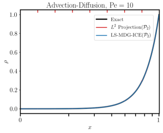
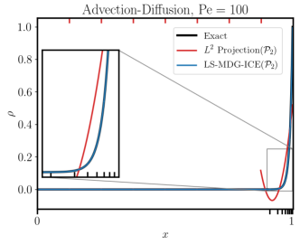
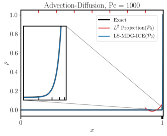
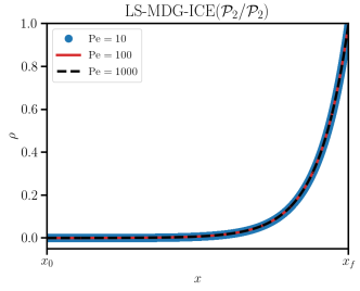
Figure 4.1: Grid adapted, self-similar solutions computed with LS-MDG-ICE$\left(\mathcal{P}_{2}\right)$ for a one-dimensional boundary layer type profile for $\mathrm{Pe}=10$, $100$, and $1000$ on a grid consisting of eight isoparametric line cells are compared to the exact solution and the $L^{2}$ projection of the exact solution onto a uniform grid. The solution was initialized with a linear profile on a uniform grid. The grid markers correspond to the adapted grid given by the LS-MDG-ICE solutions. The initial uniform grid is indicated with red tick marks. The LS-MDG-ICE$\left(\mathcal{P}_{2}/\mathcal{P}_{2}\right)$ solutions for $\mathrm{Pe}=10$, $100$, and $1000$ plotted together on rescaled domains (bottom-right).

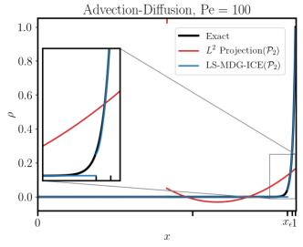
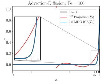
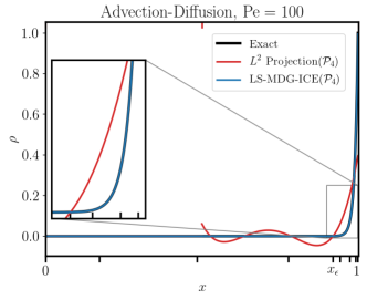
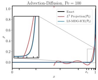
Figure 4.2: Grid adapted LS-MDG-ICE solutions for a one-dimensional boundary layer type profile for $\mathrm{Pe}=100$ on a grid consisting of two isoparametric line cells are compared to the exact solution and the $L^{2}$ projection of the exact solution onto a uniform grid. The grid markers correspond to the adapted grid and interior cell points given by the LS-MDG-ICE solutions. The interior cell interface is denoted $x_{\epsilon}$. The initial uniform grid is indicated with red tick marks.

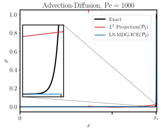
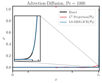
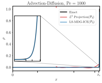
Figure 4.3: Grid adapted LS-MDG-ICE solutions for a one-dimensional boundary layer type profile for $\mathrm{Pe}=1000$ on a grid consisting of two isoparametric line cells are compared to the exact solution and the $L^{2}$ projection of the exact solution onto a uniform grid. The grid markers correspond to the adapted grid and interior cell points of the left cell given by the LS-MDG-ICE solutions. For clarity, the interior points corresponding to the right cell are not included. The interior cell interface is denoted $x_{\epsilon}$. The initial uniform grid is indicated with red tick marks.

Figure 4.1 compares the LS-MDG-ICE solutions for $\mathrm{Pe}=10,100,1000$ to the exact solution, which is numerically unstable due to round-off error for $\mathrm{Pe}=1000$, and overlays the three solutions LS-MDG-ICE solutions on rescaled domains. As expected, the solutions are self-consistent. Furthermore, the LS-MDG-ICE solutions do not exhibit oscillations in the presence of sharp gradients.

Figure 4.2 and Figure 4.3 present LS-MDG-ICE solutions on grids consisting of two isoparametric line cells for polynomial degrees $\mathcal{P}_{2}$, $\mathcal{P}_{3}$, $\mathcal{P}_{4}$, and $\mathcal{P}_{5}$ and Péclet numbers of 100 and 1000 respectively. The solutions do not exhibit oscillations, instead, under-resolved solutions are represented discontinuously, enabling highly accurate approximations of the gradient, or flux, near the boundary. Furthermore, this case demonstrates LS-MDG-ICE innate ability to not only reposition the interior cell interface, denoted $x_{\epsilon}$ in Figures 4.1, 4.1, but also nonlinearly deform the cell shape representation to improve the accuracy of the approximation. We refer to this behavior as anisotropic curvilinear $r$-adaptivity and, for the one-dimensional cases considered in this work, we will provide evidence that it enables LS-MDG-ICE to achieve super-optimal convergence with respect to the exact solution.

$\mathrm{Pe}$	$x_{\epsilon}\left(\mathcal{P}_{2}\right)$	$x_{\epsilon}\left(\mathcal{P}_{3}\right)$	$x_{\epsilon}\left(\mathcal{P}_{4}\right)$	$x_{\epsilon}\left(\mathcal{P}_{5}\right)$
$10$	$0.74756464998474681$	$0.68852737337261127$	$0.64875294047110343$	$0.53548391757202485$
$100$	$0.96910269349294942$	$0.94529226568428737$	$0.91970922330845084$	$0.89308633425846451$
$1000$	$0.99690998474116876$	$0.99452868699898989$	$0.99196943402826943$	$0.98930724837060802$
$10,000$	$0.99969099755499946$	$0.99945286890577256$	$0.99919687528580259$	$0.99892997586082066$
$100,000$	$0.99996909975446002$	$0.99994528681641881$	$0.9999196875816686$	$0.99989299759774075$

Table 1: Position of the interior interface, $x_{\epsilon}$, corresponding to LS-MDG-ICE solutions on a grid consisting of two isoparametric line cells for $\mathrm{P_{e}}=10,10^{2},10^{3},10^{4},10^{5}$. The LS-MDG-ICE solutions for $\mathrm{Pe}=10,100,1000$ are shown in Figures 4.2-4.3 respectively.

Finally, in order to verify that LS-MDG-ICE automatically solves for grids that resolve the relevant physical scales, we tabulate the positions of the interior interface, $x_{\epsilon}$, for LS-MDG-ICE solutions on a grid consisting of two isoparametric line cells in Table 1. The solutions for $\mathrm{Pe}=100,1000$ are shown in Figures 4.2-4.3 respectively, while the solutions for $\mathrm{Pe>1000}$ are not shown. In order to converge at the optimal rate, the size of the cell in the boundary layer is required to be

$$x_{r}-x_{\epsilon}\left(\mathcal{P}_{p},\mathrm{Pe}=10^{n}\right)\propto\frac{1}{\mathrm{\mathrm{Pe}}},$$ (4.3)

for Péclet numbers, $\mathrm{Pe}=\left\{10^{n}:n\in\mathbb{N}\>\mathrm{and}\>n>1\right\}$, where $x_{r}=1$ is the position of the right boundary, i.e., $x_{r}=1$. For the data presented in Table 1 indicates that LS-MDG-ICE automatically solves for grids on the diffusive scale, i.e., $\mathcal{O}\left(\varepsilon=\nicefrac{{1}}{{\mathrm{Pe}}}\right)$, overcoming a longstanding issue in optimal grid design for singularly perturbed problems.

4.1.1 Convergence for the case of linear advection-diffusion in one dimension

We present convergence results for the $L^{2}$ error of the LS-MDG-ICE approximation with respect to the exact solution (4.2) for $\mathrm{Pe}=10$.

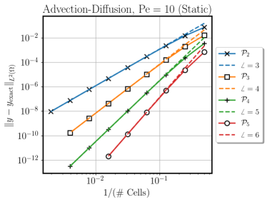
(a) Grid convergence of LS-MDG-ICE using linear line elements with a fixed discrete geometry.

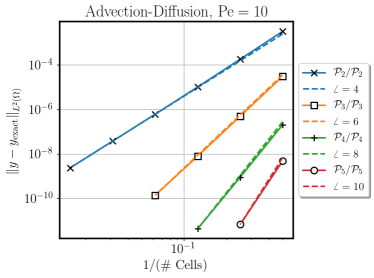
(b) Grid convergence of LS-MDG-ICE using isoparametric line elements with a variable discrete geometry.

Figure 4.4: Convergence plots for the linear advection-diffusion steady boundary layer type solution with $\mathrm{Pe}=10$ for LS-MDG-ICE($\mathcal{P}_{2}$) through LS-MDG-ICE($\mathcal{P}_{5}$) on both static and dynamic grids. On static grids the LS-MDG-ICE discretization converges with optimal ($p+1$) order. On dynamic grids, with isoparametric elements, the LS-MDG-ICE discretization converges with super-optimal ($2p$) order.

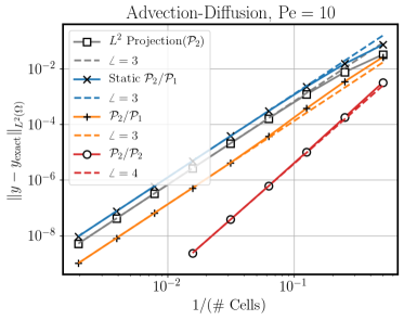
(a) LS-MDG-ICE($\mathcal{P}_{2}$) static and variable discrete geometry convergence.

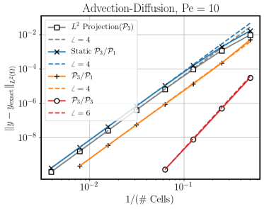
(b) LS-MDG-ICE($\mathcal{P}_{3}$) variable discrete geometry convergence.

Figure 4.5: Convergence plots for the linear advection-diffusion steady boundary layer type solution with $\mathrm{Pe}=10$ for LS-MDG-ICE($\mathcal{P}_{2}$) and LS-MDG-ICE($\mathcal{P}_{3}$). Each of the coarsest grids consisted of $2$ line cells, while the finest grid consisted of $512$, $512$, and $64$ lines cells for the static LS-MDG-ICE($\mathcal{P}_{2}/\mathcal{P}_{1}$), LS-MDG-ICE($\mathcal{P}_{2}/\mathcal{P}_{1}$), and LS-MDG-ICE($\mathcal{P}_{2}/\mathcal{P}_{2}$) discretizations respectively and $256$, $128$, and $16$ lines cells for the static LS-MDG-ICE($\mathcal{P}_{3}/\mathcal{P}_{1}$), dynamic LS-MDG-ICE($\mathcal{P}_{3}/\mathcal{P}_{1}$), and dynamic LS-MDG-ICE($\mathcal{P}_{3}/\mathcal{P}_{3}$) discretizations respectively.

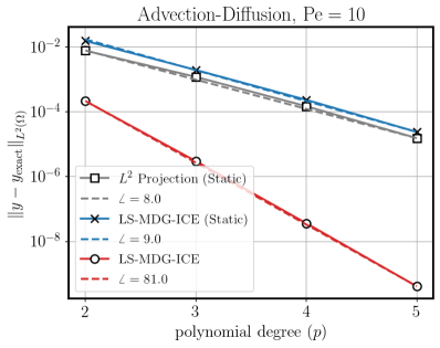
Figure 4.6: Comparison of convergence under polynomial refinement for the linear advection-diffusion steady boundary layer type solution with $\mathrm{Pe}=10$ for LS-MDG-ICE with a static and variable discrete geometry on a grid consisting of four isoparametric line elements.

Figure 4.4 presents convergence rates of LS-MDG-ICE with both a fixed and variable discrete geometry for polynomial degrees $p=2,\ldots,5$. The coarsest grid consists of $2$ line cells, while the finest grid consists of $256$ line cells. For a fixed discrete geometry, LS-MDG-ICE exhibits optimal $\left(p+1\right)$ order convergence. For a variable discrete geometry, LS-MDG-ICE exhibits super-optimal $\left(2p\right)$ order convergence.

Figure 4.5 directly compares the convergence rates of LS-MDG-ICE with a fixed and variable discrete geometry for $p=2,3$. For reference, we have also included the error associated with the $L^{2}$ projection of the exact solution onto a uniform grid, which provides an upper bound on the accuracy attainable by methods based on a static grid since it minimizes the error in the $L^{2}$ norm. For the case of a variable discrete geometry, we consider both linear and isoparametric line elements in order. In the case of linear line elements LS-MDG-ICE exhibits the same optimal $\left(p+1\right)$ order convergence as the case of a fixed discrete geometry. However, the solution is almost 8 times more accurate. The solution is most accurate for the case of isoparametric line cells. The LS-MDG-ICE($\mathcal{P}_{3}$) requires $256$, $128$, and $16$ line cells to achieve an error on the order of $10^{-9}$ for the case of a static discrete geometry, variable linear discrete geometry, and variable isoparametric discrete geometry.

Figure 4.9 compares convergence of LS-MDG-ICE solutions under polynomial refinement for $\mathrm{Pe}=10$ on grids consisting of four line cells for the case of static discrete geometry and variable isoparametric discrete geometry. Again, we include the error associated with the $L^{2}$ projection of the exact solution onto a uniform grid for reference. The $L^{2}$ projection, static LS-MDG-ICE, and LS-MDG-ICE errors are plotted on a log-linear plot, with a reference slope of $8$, $9$, and $81$, respectively.

4.2 Burgers steady viscous shock

We consider the solution of the nonlinear conservation law in one dimension corresponding to the viscous Burgers equation [55, 56]. The exact solution is given by

$$y\left(x\right)=y_{R}+\frac{1}{2}\left(y_{L}-y_{R}\right)\left(1-\tanh\left(\frac{\left(y_{L}-y_{R}\right)\left(x-v_{s}t\right)}{4\epsilon}\right)\right)$$ (4.4)

where

$$v_{s}=\frac{1}{2}\left(y_{L}+y_{R}\right)$$ (4.5)

is the shock speed, $\epsilon$ is a viscosity coefficient, and $t$ is the time. The boundary conditions at $x=\pm\nicefrac{{1}}{{2}}$ are given by Equation (4.4), which results in a stationary viscous shock, i.e., $v_{s}=0$. The solutions is initialized with a piecewise constant profile

$$y\left(x\right)=\begin{cases}y\left(\nicefrac{{-1}}{{2}}\right)&\textup{ if }x_{c}\leq 0\\ y\left(\nicefrac{{+1}}{{2}}\right)&\textup{ if }x_{c}>0\end{cases}$$ (4.6)

where $x_{c}$ is the cell centroid. For certain parameter regimes, $\epsilon\leq 10^{-3}$, the solution to the problem is not unique since perturbations to the boundary data are smaller than machine precision [17].

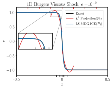
(a) LS-MDG-ICE$\left(\mathcal{P}_{2}\right)$

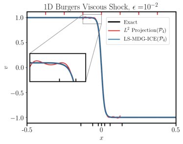
(b) LS-MDG-ICE$\left(\mathcal{P}_{4}\right)$

Figure 4.7: Burgers steady viscous shock solutions for $\epsilon=10^{-2}$ computed with LS-MDG-ICE$\left(\mathcal{P}_{2}\right)$ and LS-MDG-ICE$\left(\mathcal{P}_{4}\right)$ on eight isoparametric line cells. The solutions were initialized on a uniform grid with a piecewise constant profile given by Equation (4.6). The initial grid points are marked with red ticks on the top of the plots and the adapted grid points given by the LS-MDG-ICE solutions are marked with black ticks on the bottom of the plots.

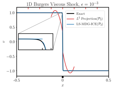
(a) LS-MDG-ICE$\left(\mathcal{P}_{2}\right)$

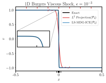
(b) LS-MDG-ICE$\left(\mathcal{P}_{4}\right)$

Figure 4.8: Burgers steady viscous solutions shock for $\epsilon=10^{-3}$ computed with LS-MDG-ICE$\left(\mathcal{P}_{2}\right)$ and LS-MDG-ICE$\left(\mathcal{P}_{4}\right)$ on eight isoparametric line cells. The solutions were initialized on a uniform grid with a piecewise constant profile given by Equation (4.6). The initial grid points are marked with red ticks on the top of the plots and the adapted grid points given by the LS-MDG-ICE solutions are marked with black ticks on the bottom of the plots.

Figure 4.7 and Figure 4.8 present Burgers steady viscous shock solutions for $\epsilon=10^{-2}$ and $\epsilon=10^{-3}$ computed with LS-MDG-ICE$\left(\mathcal{P}_{2}\right)$ and LS-MDG-ICE$\left(\mathcal{P}_{4}\right)$ on eight isoparametric line cells. The $L^{2}$ projection of the exact solution (4.4) onto a uniform grid is plotted as well and the initial uniform grid is marked with red ticks. The LS-MDG-ICE solutions do not contain oscillations, a problematic feature of under-resolved polynomial approximations, which can be seen in the $L^{2}$ projection of the exact solution. The discontinuities present in the LS-MDG-ICE$\left(\mathcal{P}_{2}\right)$ solutions shown in Figure 4.7b and Figure 4.8b provide a mechanism for accurately representing under-resolved features, which localizes the error, and prevents it from polluting the solution upstream. Furthermore, as the approximation order is increased, the unphysical discontinuities are resolved and the LS-MDG-ICE solution becomes indistinguishable from the exact solution. Figure 4.7b and Figure 4.8b present the LS-MDG-ICE$\left(\mathcal{P}_{4}\right)$ solution computed on eight isoparametric line cells for $\epsilon=10^{-2}$ and $\epsilon=10^{-3}$ respectively.

4.2.1 Convergence for the case of viscous Burgers flow in one dimension

Figure 4.9: Convergence plot for Burgers steady viscous shock with $\epsilon=10^{-2}$ using LS-MDG-ICE($\mathcal{P}_{2}$) isoparametric elements. The coarsest grid consists of $10$ isoparametric line elements and the finest grid consists of $80$ isoparametric line elements.

Figure 4.9 presents convergence results under grid refinement for Burgers steady viscous shock at $\epsilon=10^{-2}$ using LS-MDG-ICE($\mathcal{P}_{2}$). The coarsest grid consists of $10$ isoparametric line elements and the finest grid consists of $80$ isoparametric line elements. At these moderate conditions, an excessively fine grid resolution is required to obtain the optimal convergence rate under uniform refinement. This lack of resolution is manifested in the error associated with the $L^{2}$ projection of the exact solution, which converges sub-optimally with a rate of $2.5$. In contrast, LS-MDG-ICE adapts the grid to resolve the relevant physical scales and therefore overcomes the challenges associated with traditional methods based on static grids. In fact, LS-MDG-ICE again achieves super-optimal convergence at the rate of $2p$ in the case of variable isoparametric discrete geometry. For static grid methods, the use of a layer adapted grid, where the grid is non-uniformly refined, or graded, to produce higher resolution in regions with steep gradients, could, at best, restore optimal convergence rates.

4.3 Compressible Navier-Stokes steady viscous shock

We present the solution to a one-dimensional viscous shock for a compressible Navier-Stokes flow in order to verify the nonlinear viscous flux formulation and implementation. The initial left and right states, as well as the boundary conditions, i.e., $y\left(x=-1\right)$ and $y\left(x=-1\right)$, are given as

$$\left(\rho,v,T\right)\left(x\right)=\begin{cases}\left(1,3.5,1\right)&x<0\\ \left(4.260869565217392,0.8214285714285714,3.3150510204081627\right)&x>0\end{cases},$$ (4.7)

where the right state was derived such that the jump conditions given by Equation (3.18) are satisfied. In one dimension, the problem reduces to a system of ordinary differential equations that can be solved numerically, see [17, 57] for details.

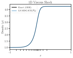
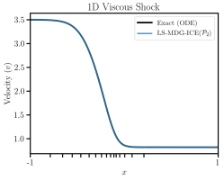
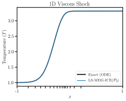
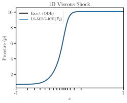
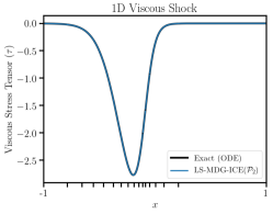
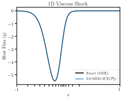
Figure 4.10: The LS-MDG-ICE($\mathcal{P}_{2}$) computed on 16 isoparametric line cells for steady viscous Mach 3.5 shock at $\mathrm{Re}=25$, $\mathrm{Pr}=0.72$, and $T_{\infty}=293.15$ .

Figure 4.10 presents the LS-MDG-ICE($\mathcal{P}_{2}$) solution computed on 16 isoparametric line cells and the ODE approximation of the exact solution computed using fourth-order ODE integration with a step size of $10^{-4}$ for a steady viscous Mach 3.5 shock at $\mathrm{Re}=25$, $\mathrm{Pr}=0.72$, and $T_{\infty}=293.15$. The location of the viscous shock corresponding to the initial conditions given by Equation (4.7) is not uniquely determined. The numerical approximation to the set of ODEs describing the exact solution was shifted by $x=-0.14$ and extrapolated to the right boundary, $x=1$, for direct comparison with the LS-MDG-ICE solution. Figure 4.10 also shows the final grid projected to the space $\mathcal{P}_{1}$, which adapted to resolve multiple profiles simultaneously, providing the highest resolution at the transition from the viscous shock to the right state where oscillations generated by traditional methods based on polynomial approximations are expected to be the greatest.

4.4 Sinusoidal Waves

(a) Spatial velocity $v_{x}=\frac{1}{10}$. Reproduction of the convergence results originally presented in our previous work using a discrete least-squares solver with an equal-order test space [2]

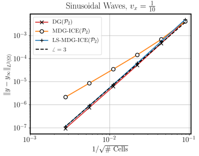
(b) Spatial velocity $v_{x}=\frac{1}{10}$. Optimal-order convergence results obtained using LS-MDG-ICE($\mathcal{P}_{2}$)

Figure 4.11: Convergence plots for linear advection of a smooth sinusoidal wave comparing a standard DG($\mathcal{P}_{2}$) method with an MDG-ICE($\mathcal{P}_{2}$) method using the discrete weak formulation given by Equation (6.5) in [2]. The coarsest grid consisted of $128$ triangle cells, while the finest grid consisted of $131,072$ triangle cells. For this smooth flow the discrete geometry $u$ is fixed. For the case of a spatial velocity $v_{x}=\frac{1}{10}$, unweighted MDG-ICE($\mathcal{P}_{2}$) converges at a sub-optimal rate, while DG($\mathcal{P}_{2}$), weighted MDG-ICE($\mathcal{P}_{2}$), and LS-MDG-ICE($\mathcal{P}_{2}$) achieve optimal third-order convergence.

We revisit two-dimensional linear advection of a sinusoidal wave presented in [2] and demonstrate that LS-MDG-ICE achieves optimal-order convergence with respect to grid refinement on a static, two-dimensional grid. This problem involves a smooth flow defined over the space-time domain $\Omega=\left(0,2\right)\times\left(0,2\right)$, governed by the linear advection equation, cf. Section 3.1.1, with a spatial velocity $v_{x}>0$ and diffusion coefficient $\epsilon=0$. The exact solution

$$y\left(x,t\right)=\frac{7}{5}\left(1+\frac{1}{10}\sin\left(2\pi\left(x-v_{x}t\right)\right)\right),$$ (4.8)

is used to define temporal inflow (initial) and spatial inflow boundary conditions at $t=0$ and $x=0$.

Figure 4.11 presents convergence results with respect to grid refinement for the case of $v_{x}=0.1$. The initial coarse grid consisted of $128$ triangle cells and was refined successively up to $131,072$ triangle cells. Figure 4.11a reproduces the convergence results corresponding to DG($\mathcal{P}_{2}$), MDG-ICE($\mathcal{P}_{2}$), and weighted MDG-ICE($\mathcal{P}_{2}$) originally presented in our earlier work [2]. In this case, unweighted MDG-ICE($\mathcal{P}_{2}$) converges at a sub-optimal rate, while both DG($\mathcal{P}_{2}$) and weighted MDG-ICE($\mathcal{P}_{2}$) achieve optimal third-order convergence. Optimal third-order convergence is recovered for MDG-ICE if the interface term is scaled by a coefficient $\alpha_{h}\in\mathbb{R}$, which, for this particular problem, is defined as

$$\alpha_{h}=2^{i},$$ (4.9)

for $i=0,\cdots,n$, where $n$ is the number of times the solution was refined. Thus, $\alpha_{h}$ is one on the coarsest level and increases by a factor of two upon each level of refinement. This formulation is referred to as weighted-MDG-ICE($\mathcal{P}_{2}$) in Figure 4.11a.

The interface weight $\alpha_{h}$ that will recover optimal-order convergence is unknown in general. In contrast, the least-squares formulation uses optimal test functions that are generated automatically and do not require an ad hoc scaling. Figure 4.11b replaces weighted MDG-ICE with LS-MDG-ICE. As expected, LS-MDG-ICE converges at the optimal rate and is comparable to DG($\mathcal{P}_{2}$) in terms of accuracy. The error with respect to the exact solution on the finest grid is $1.14\times 10^{-7}$ for LS-MDG-ICE and $9.36\times 10^{-8}$ DG($\mathcal{P}_{2}$).

4.5 Inviscid Mach 3 bow shock

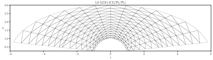
(a) 392 isoparametric $\mathcal{P}_{2}$ triangle cells

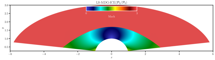
(b) 392 isoparametric $\mathcal{P}_{2}$ triangle cells

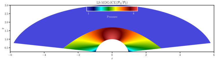
(c) 392 isoparametric $\mathcal{P}_{2}$ triangle cells

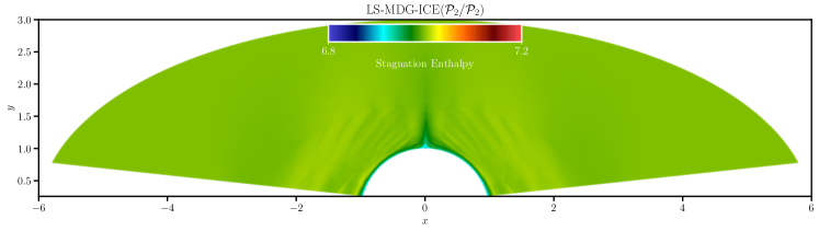
(d) 392 isoparametric $\mathcal{P}_{2}$ triangle cells

Figure 4.12: Inviscid Mach 3 bow shock: The LS-MDG-ICE solution computed using $\mathcal{P}_{2}$ isoparametric triangle elements. The LS-MDG-ICE field variables were initialized by projecting the cell averaged DG($\mathcal{P}_{2}$) solution. The location of the shock along the line $x=0$ was computed as $y=1.698$ for a stand-off distance of $0.698$. The error of the stagnation enthalpy, $\left\|H-H_{\infty}\right\|_{L^{2}\left(\Omega\right)}$, with respect to the exact solution, $H_{\infty}=7$, is $2.2736\times 10^{-2}$.

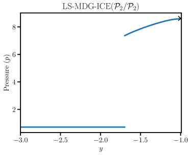
(a) The pressure sampled along $x=0$. The exact pressure at the stagnation point, $p\approx 8.614975$, is marked with the symbol $\times$. The computed pressure at the stagnation point on is $8.585034$.

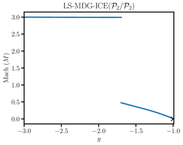
(b) The Mach number sampled along $x=0$. The exact Mach number at the stagnation point, $M=0$, is marked with the symbol $\times$. The computed Mach number at the stagnation point is $6.86725\times 10^{-3}$.

Figure 4.13: Inviscid Mach 3 bow shock: Computed with LS-MDG-ICE using $\mathcal{P}_{2}$ isoparametric triangle elements. The location of the shock was computed as $y=1.698$ for a stand-off distance of $0.698$.

The least-squares formulation was applied to the steady inviscid Mach 3 bow shock. Figure 4.12 presents the final mesh, temperature, pressure, and stagnation enthalpy fields corresponding to the MDG-ICE($\mathcal{P}_{2}$) solution computed using $392$ $\mathcal{P}_{2}$ isoparametric triangle elements. The field variables were initialized by projecting the cell averaged DG($\mathcal{P}_{2}$) solution. The error of the stagnation enthalpy, $\left\|H-H_{\infty}\right\|_{L^{2}\left(\Omega\right)}$, with respect to the exact solution, $H_{\infty}=7$, was reduced from $4.0932\times 10^{-1}$ to $2.2736\times 10^{-2}$. The stand off distance was estimated to be to $0.698$, which is in agreement with the estimate computed using the discrete least-squares formulation reported previously [2].

Figure 4.13 presents the pressure and Mach number sampled along the centerline, $x=0$. The computed pressure at the stagnation point is $8.585034$. The exact pressure at the stagnation point, $p\approx 8.614975$, is marked with the symbol $\times$ in Figure 4.13a. The computed Mach number at the stagnation point is $M=6.86725\times 10^{-3}$. The exact Mach number at the stagnation point, $M=0$, is marked with the symbol $\times$ in Figure 4.13a

4.6 Viscous Mach 5 bow shock

To verify the viscous LS-MDG-ICE discretization of compressible Navier-Stokes flow, as described in Section 3.1.3, and demonstrate the ability of the LS-MDG-ICE to simultaneously resolve both the interior viscous shock and viscous boundary layer via anisotropic curvilinear $r$-adaptivity. We consider Mach 5 flows at a Reynolds numbers of $10^{3}$ and $10^{4}$ and extend the one-dimensional analysis from [3] to the case of $\mathrm{Re}=10^{4}$.

A supersonic viscous flow over a cylinder in two dimensions is characterized by the Reynolds number $\mathrm{Re}$, and the freestream Mach number $M_{\infty}$. The Reynolds number is defined as,

$$\mathrm{Re}=\frac{\rho vL}{\mu},$$ (4.10)

where $L$ is the characteristic length. The freestream Mach number is defined $M_{\infty}=\frac{v_{\infty}}{c_{\infty}}$

$$M_{\infty}=\frac{v_{\infty}}{c_{\infty}},$$ (4.11)

where $v_{\infty}$ is the freestream velocity, $c_{\infty}=\sqrt{\nicefrac{{\gamma P_{\infty}}}{{\rho_{\infty}}}}$ is the freestream speed of sound, $P_{\infty}$ is the freestream pressure, and $\rho_{\infty}$ is the freestream density. In this work, we assume the flow is traveling in the negative $y$-direction, i.e., from top to bottom in Figure 4.14 and Figure 4.17. Supersonic inflow and outflow boundary conditions are applied on the ellipse boundary, which is defined by $\left(\nicefrac{{x}}{{3}}\right)^{2}+\left(\nicefrac{{y}}{{6}}\right)^{2}=1$, and outflow planes respectively. An isothermal no-slip wall is specified at the surface of the cylinder of radius $r=1$, centered at the origin. The temperature at the isothermal wall is given as $T_{\mathrm{wall}}=2.5T_{\infty}$, where $T_{\infty}$ is the freestream temperature.

We follow the approach described in [3] and use local edge refinement to adaptively split highly anisotropic elements within the viscous structures as they were resolved by LS-MDG-ICE. This simple approach is highly effective for maintaining the original grid resolution downstream of the viscous shock, which becomes less resolved as the solver moves the grid to anisotropically resolve the shock, as well as for inserting additional degrees of freedom in order to better resolve the curved shock geometry.

Furthermore, we follow the approach of Zahr et al. [32] and incorporate the local cell size into the regularization by scaling $\lambda_{u}$ of (3.76) by a factor proportional to the inverse of the element volume. This allowed for more aggressive grid motion, as highly anisotropic elements were less likely to degenerate as the grid points were repositioned to resolve the sharp viscous features. The result is a coarser grid in the region upstream of the viscous shock where the flow is constant and finer grid resolution through the viscous shock as compared to the corresponding solution shown in Figure 3.5  of [3], which did not weight $\lambda_{u}$ by the inverse cell volume.

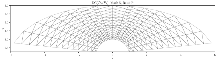
(a) 392 $\mathcal{P}_{1}$-shape triangle cells

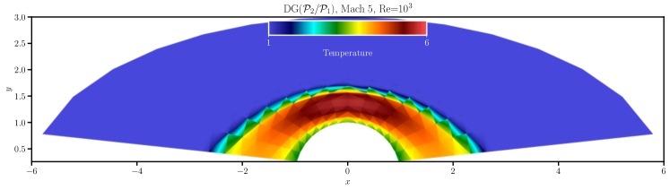
(b) 392 linear $\mathcal{P}_{2}$ triangle cells

Figure 4.14: The initial linear grid and temperature field corresponding to a shock captured DG($\mathcal{P}_{2}/\mathcal{P}_{1}$) solution for the viscous Mach 5 bow shock at $\mathrm{Re}=10^{3}$.

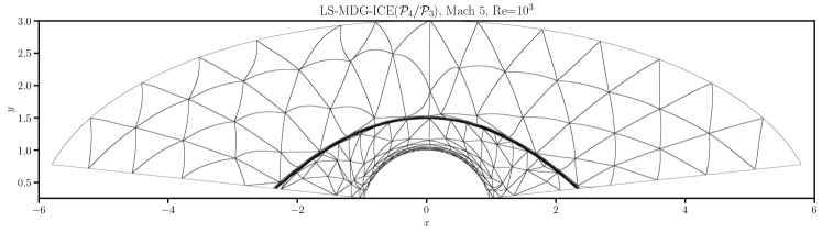
(a) 502 sub-parametric $\mathcal{P}_{4}/\mathcal{P}_{3}$ triangle cells

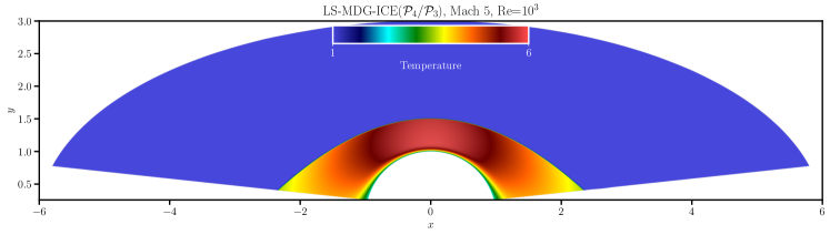
(b) 502 sub-parametric $\mathcal{P}_{4}/\mathcal{P}_{3}$ triangle cells

(c) 502 sub-parametric $\mathcal{P}_{4}/\mathcal{P}_{3}$ triangle cells

(d) 502 sub-parametric $\mathcal{P}_{4}/\mathcal{P}_{3}$ triangle cells

Figure 4.15: The LS-MDG-ICE solution computed using $\mathcal{P}_{4}/\mathcal{P}_{3}$ sub-parametric triangle elements for the viscous Mach 5 bow shock at $\mathrm{Re}=10^{3}$. The LS-MDG-ICE grid was initialized by projecting the linear triangle grid shown in Figure 4.14a. The LS-MDG-ICE field variables were initialized by projecting the cell-averaged DG($\mathcal{P}_{2}/\mathcal{P}_{1}$) solution shown in Figure 4.14b. The LS-MDG-ICE flux variables were initialized to zero for consistency with the initial piecewise constant field variables. The location of the shock along the line $x=0$ was computed as $y=1.5000575$ for a stand-off distance of $0.5000575$.

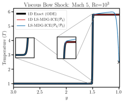
(a) The exact temperature at the stagnation point, $T=2.5$, is marked with the symbol $\times$.

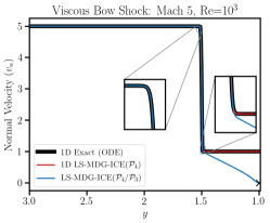
(b) The exact normal velocity at the stagnation point, $v_{n}=0$, is marked with the symbol $\times$.

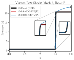
(c) The exact pressure at the stagnation point for an inviscid flow, $p\approx 23.324$, is marked with the symbol $\times$.

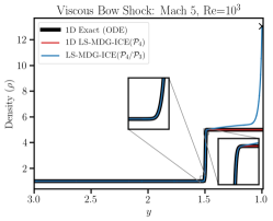
(d) The density at the stagnation point, computed using the stagnation pressure corresponding to an inviscid flow, $\rho\approx 13.0614$, is marked with the symbol $\times$.

(e) The normal component of the normal viscous stress tensor, $\tau_{nn}$.

(f) The normal thermal heat flux, $q_{n}$.

Figure 4.16: Centerline profiles, sampled along $x=0$, for the viscous Mach 5 bow shock at $\mathrm{Re}=10^{3}$ computed with LS-MDG-ICE($\mathcal{P}_{4}/\mathcal{P}_{3}$) compared to ODE and MDG-ICE($\mathcal{P}_{4}$) approximations of the exact solution for the corresponding one-dimensional viscous shock. The one-dimensional LS-MDG-ICE($\mathcal{P}_{4}$) approximation was computed using 16 isoparametric line cells. The location of the shock was computed as as $y=1.5000575$ for a stand-off distance of $0.5000575$.

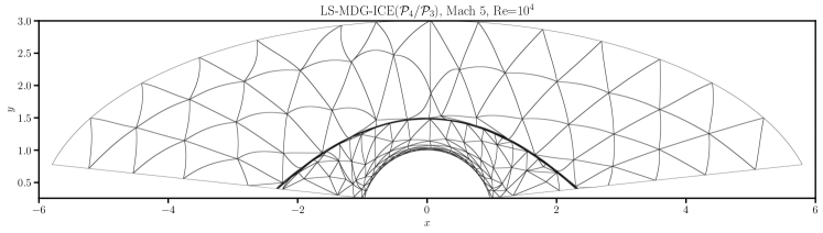
(a) 508 sub-parametric $\mathcal{P}_{4}/\mathcal{P}_{3}$ triangle cells

(b) 508 sub-parametric $\mathcal{P}_{4}/\mathcal{P}_{3}$ triangle cells

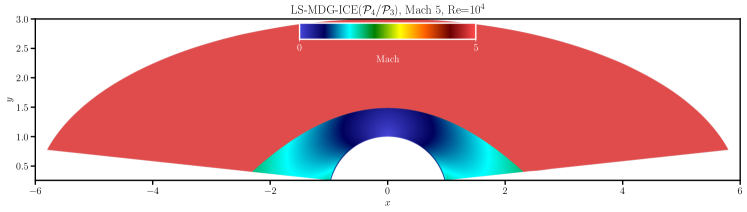
(c) 508 sub-parametric $\mathcal{P}_{4}/\mathcal{P}_{3}$ triangle cells

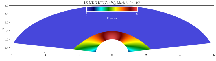
(d) 508 sub-parametric $\mathcal{P}_{4}/\mathcal{P}_{3}$ triangle cells

Figure 4.17: The LS-MDG-ICE solution computed using $\mathcal{P}_{4}/\mathcal{P}_{3}$ sub-parametric triangle elements for the viscous Mach 5 bow shock at $\mathrm{Re}=10^{4}$. The MDG-ICE solution was initialized from the LS-MDG-ICE solution at $10^{3}$ $\mathrm{Re}$ shown in Figure 4.14a. The location of the shock along the line $x=0$ was computed as $y=1.4847275$ for a stand-off distance of $0.4847275$.

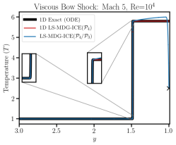
(a) The temperature sampled along $x=0$. The exact temperature at the stagnation point, $T=2.5$, is marked with the symbol $\times$.

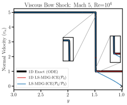
(b) The normal velocity, $v_{n}=0$, sampled along $x=0$. The exact normal velocity at the stagnation point, $v_{n}=0$, is marked with the symbol $\times$.

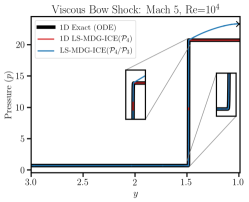
(c) The pressure, $p$, sampled along $x=0$. The exact pressure at the stagnation point for an inviscid flow, $p\approx 23.324$, is marked with the symbol $\times$.

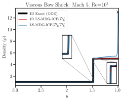
(d) The density, $\rho$, sampled along $x=0$. The density at the stagnation point, computed using the stagnation pressure corresponding to an inviscid flow, $\rho\approx 13.061$, is marked with the symbol $\times$.

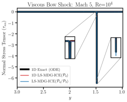
(e) The normal component of the normal viscous stress tensor, $\tau_{nn}$, sampled along $x=0$.

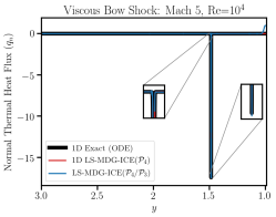
(f) The normal thermal heat flux, $q_{n}$, sampled along $x=0$.

Figure 4.18: Centerline profiles of temperature and normal velocity for the viscous Mach 5 bow shock at $\mathrm{Re}=10^{4}$ computed with LS-MDG-ICE($\mathcal{P}_{4}/\mathcal{P}_{3}$) compared to ODE and LS-MDG-ICE($\mathcal{P}_{4}$) approximations of the exact solution for the corresponding one-dimensional viscous shock. The one-dimensional LS-MDG-ICE($\mathcal{P}_{4}$) approximation was computed using 16 isoparametric line cells. The location of the shock along the line $x=0$ was computed as $y=1.4847275$ for a stand-off distance of $0.4847275$.

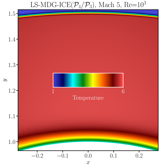
(a) The final grid and temperature fields of the LS-MDG-ICE$\left(\mathcal{P}_{4}\right)$ solution computed using 502 $\mathcal{P}_{4}$ isoparametric triangle elements for the viscous Mach 5 bow shock at $\mathrm{Re}=10^{3}$ shown in Figure 4.15a and Figure 4.15b respectively.

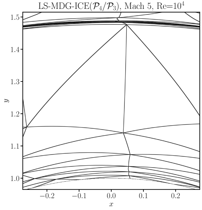
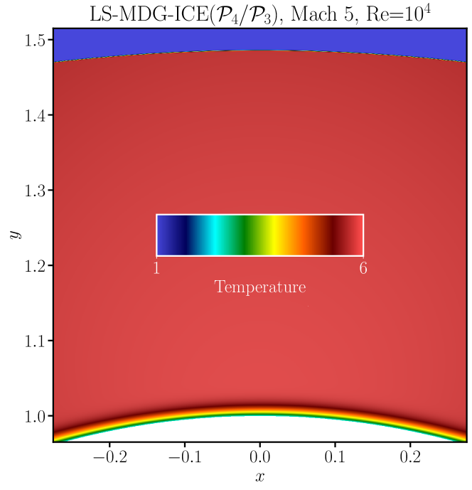
(b) The final grid and temperature fields of the LS-MDG-ICE$\left(\mathcal{P}_{4}\right)$ solution computed using 508 $\mathcal{P}_{4}$ isoparametric triangle elements for the viscous Mach 5 bow shock at $\mathrm{Re}=10^{4}$ shown in Figure 4.17a and Figure 4.17b.

Figure 4.19: The final grid and temperature fields corresponding to the LS-MDG-ICE solution computed using $\mathcal{P}_{4}$ isoparametric triangle elements for the viscous Mach 5 bow shock at $\mathrm{Re}=10^{3}$ and $\mathrm{Re}=10^{4}$. Local edge refinement was used to adaptively split highly anisotropic elements within the viscous structures as they were resolved by LS-MDG-ICE.

The one-dimensional viscous shock solution, as described in Section 4.3, is used to verify that the viscous LS-MDG-ICE formulation predicts the correct viscous shock profile when diffusive effects are prominent. Figure 4.16 and Figure 4.18 compare an approximation of the exact solution for a one-dimensional viscous shock to the centerline profiles of the Mach 5 bow shock at $\mathrm{Re}=10^{3}$ and $\mathrm{Re}=10^{4}$, respectively, for the following variables: temperature, $T$, normal velocity, $v_{n}$, pressure, $p$, density, $\rho$, normal component of the normal viscous stress tensor, $\tau_{nn}$, and normal heat flux, $q_{n}$, where the normal is taken to be in the in the streamwise direction. For reference and to aid comparisons to the exact solution, we also plotted the LS-MDG-ICE($\mathcal{P}_{4}$) solution to the one-dimensional viscous shock problem computed using 16 isoparametric line cells. For reference, the exact and approximate values at the stagnation point are marked on the centerline plots with the symbol $\times$. When the exact value for the viscous flow was unavailable we approximate it with the value corresponding to the inviscid solution, which is not expected to differ significantly for the cases considered here, see [58, Table 1].

As noted in [3], the viscous shock profile corresponding to the one-dimensional solution is expected to deviate from the bow shock centerline profiles downstream of the viscous shock where the viscous effects are produced by the boundary layer associated with the blunt body centered at the origin. The jump across the viscous shock is directly comparable to the one-dimensional solution in the case of density, for which the viscous flux is zero. Figure 4.16d shows that LS-MDG-ICE accurately reproduces the density profile of the exact shock structure with only a few anisotropic high-order cells.

The ability of LS-MDG-ICE($\mathcal{P}_{4}/\mathcal{P}_{3}$) to resolve viscous layer using anisotropic curvilinear $r$-adaptivity is further demonstrated in Figure 4.19 where the solutions between the viscous shock and the blunt body for $\mathrm{Re}=10^{3}$ and $\mathrm{Re}=10^{4}$ are compared. This feature was showcased in [3, Section 3.3] and was further explored in Section 4.1 for the case of one-dimensional advection-diffusion where it enabled LS-MDG-ICE to achieve super-optimal convergence rates on the order of $2p$. Here we again demonstrate it naturally extends to multiple dimensions where LS-MDG-ICE automatically repositions the points in order to resolve the flow field over the relevant physical length scales.

Conclusions and future work

The Discontinuous Petrov-Galerkin (DPG) methodology of Demkowicz and Gopalakrishnan was used to derive a least-squares formulation of MDG-ICE with optimal test functions, which were systematically generated from the trial spaces of both the discrete flow field and discrete geometry. The LS-MDG-ICE formulation inherits unique and desirable features of the (DLS) MDG-ICE formulation used in [2, 3], such as the ability to fit a priori unknown interfaces and resolve sharp, but smooth, viscous flow features using anisotropic curvilinear $r$-adaptivity. Additionally, for both linear and nonlinear problems in one dimension, the LS-MDG-ICE discretization was verified to converge with optimal ($p+1$) and super-optimal ($2p$) order under grid refinement for polynomial spaces $\mathcal{P}_{2}$ through $\mathcal{P}_{5}$ using a static, or fixed, discrete geometry and a variable discrete geometry. We also observed optimal-order convergence for a steady, two-dimensional linear advection problem.

In two dimensions , the LS-MDG-ICE formulation is capable of producing highly accurate solutions for problems involving curved interface topologies and sharp viscous layers. For the Mach 3 inviscid bow, LS-MDG-ICE accurately fit the curved shock and the computed stand-off distance compared well to the value reported previously [2]. The LS-MDG-ICE($\mathcal{P}_{2}$) solution was accurate and oscillation-free on a grid consisting of only 392 isoparametric triangle cells. Local grid operations, i.e., edge refinement and collapse, were not required to fit the curved interface.

The first-order system LS-MDG-ICE formulation for viscous flows was used to approximate a Mach 5 viscous Bow shock at $\mathrm{Re}=10^{3}$ and $\mathrm{Re}=10^{4}$. The one-dimensional analysis from our previous work [3] was reproduced for the case of $\mathrm{Re}=10^{3}$ and it was extended to the case of $\mathrm{Re}=10^{4}$. The centerline profiles through the viscous shock were in agreement with the ODE and one-dimensional LS-MDG-ICE($\mathcal{P}_{4}$) approximations of the exact one-dimensional viscous shock profile. For the case of $\mathrm{Re}=10^{3}$, the estimated stand off distance of $0.5000575$ compares well to the previously reported MDG-ICE standoff distance of $0.49995$. For these challenging problems, we scaled the linear elastic grid regularization by a factor similar to the one introduced by Zahr et al. [32] that is proportional to the inverse of the element volume, which helped prevent cells from degenerating as the solver simultaneously resolved the viscous shock and boundary layer via anisotropic curvilinear $r$-adaptivity.

Future work will analyze the proposed method in a rigorous setting and further study its ability to achieve optimal-order convergence in the case of higher-dimensional, nonlinear problems.

References

- [1] A. Corrigan, A. Kercher, D. Kessler, A moving discontinuous Galerkin finite element method for flows with interfaces, Tech. Rep. NRL/MR/6040–17-9765, U.S. Naval Research Laboratory, https://apps.dtic.mil/dtic/tr/fulltext/u2/1042881.pdf (December 2017).
- [2] A. Corrigan, A. Kercher, D. Kessler, A moving discontinuous Galerkin finite element method for flows with interfaces, International Journal for Numerical Methods in Fluids 89 (9) (2019) 362–406. doi:10.1002/fld.4697.
- [3] A. Kercher, A. Corrigan, D. Kessler, The moving discontinuous Galerkin finite element method with interface condition enforcement for compressible viscous flows (2020). arXiv:2002.12740.
- [4] B. Keith, S. Petrides, F. Fuentes, L. Demkowicz, Discrete least-squares finite element methods, Computer Methods in Applied Mechanics and Engineering 327 (2017) 226–255. doi:10.1016/j.cma.2017.08.043.
- [5] L. Demkowicz, J. Gopalakrishnan, A class of discontinuous Petrov–Galerkin methods. part I: The transport equation, Computer Methods in Applied Mechanics and Engineering 199 (23-24) (2010) 1558–1572. doi:10.1016/j.cma.2010.01.003.
- [6] L. Demkowicz, J. Gopalakrishnan, A class of discontinuous Petrov–Galerkin methods. II. optimal test functions, Numerical Methods for Partial Differential Equations 27 (1) (2011) 70–105. doi:10.1002/num.20640.
- [7] L. Demkowicz, J. Gopalakrishnan, A. H. Niemi, A class of discontinuous Petrov–Galerkin methods. part III: Adaptivity, Applied numerical mathematics 62 (4) (2012) 396–427. doi:10.1016/j.apnum.2011.09.002.
- [8] L. Demkowicz, Various variational formulations and closed range theorem, Tech. Rep. 15-03, ICES, retrieved from https://www.oden.utexas.edu/media/reports/2015/1503.pdf (January 2015).
- [9] L. Demkowicz, J. Gopalakrishnan, Discontinuous Petrov-Galerkin (DPG) method, Tech. Rep. 15-20, ICES, retrieved from https://www.oden.utexas.edu/media/reports/2015/1520.pdf (October 2015).
- [10] L. Demkowicz, J. Gopalakrishnan, B. Keith, The DPG-star method, Computers & Mathematics with Applicationsdoi:10.1016/j.camwa.2020.01.012.
- [11] J. Gopalakrishnan, Five lectures on DPG methods (2013). arXiv:1306.0557.
- [12] J. Gopalakrishnan, W. Qiu, An analysis of the practical DPG method, Mathematics of Computation 83 (286) (2014) 537–552.
- [13] C. Carstensen, L. Demkowicz, J. Gopalakrishnan, Breaking spaces and forms for the DPG method and applications including Maxwell equations, Computers & Mathematics with Applications 72 (3) (2016) 494–522. doi:10.1016/j.camwa.2016.05.004.
- [14] Z. Cai, R. Lazarov, T. Manteuffel, S. McCormick, First–order system least squares for second–order partial differential equations: Part i, SIAM Journal on Numerical Analysis 31 (6) (1994) 1785–1799. doi:10.1137/0731091.
- [15] P. Bochev, M. Gunzburger, Finite element methods of least-squares type, SIAM review 40 (4) (1998) 789–837. doi:10.1137/S0036144597321156.
- [16] P. Bochev, M. Gunzburger, Least–squares finite element methods, Springer Science & Business Media, 2009. doi:10.1007/b13382.
- [17] J. Chan, L. Demkowicz, R. Moser, N. Roberts, A new discontinuous Petrov-Galerkin method with optimal test functions. part V: solution of 1D Burgers’ and Navier-Stokes equations, Tech. Rep. 10-25, ICES, retrieved from https://www.oden.utexas.edu/media/reports/2010/1025.pdf (June 2010).
- [18] J. Chan, L. Demkowicz, R. Moser, A DPG method for steady viscous compressible flow, Computers & Fluids 98 (2014) 69–90. doi:10.1016/j.compfluid.2014.02.024.
- [19] N. V. Roberts, T. Bui-Thanh, L. Demkowicz, The DPG method for the Stokes problem, Computers & Mathematics with Applications 67 (4) (2014) 966–995. doi:10.1016/j.camwa.2013.12.015.
- [20] N. Roberts, L. Demkowicz, R. Moser, A discontinuous Petrov–Galerkin methodology for adaptive solutions to the incompressible Navier–Stokes equations, Journal of Computational Physics 301 (2015) 456–483. doi:10.1016/j.jcp.2015.07.014.
- [21] T. Bui-Thanh, L. Demkowicz, O. Ghattas, A unified discontinuous Petrov–Galerkin method and its analysis for Friedrichs’ systems, SIAM Journal on Numerical Analysis 51 (4) (2013) 1933–1958. doi:10.1137/110854369.
- [22] M. Gerritsma, M. Proot, Analysis of a discontinuous least squares spectral element method, Journal of Scientific Computing 17 (1-4) (2002) 297–306. doi:10.1023/A:1015121219065.
- [23] Y. Cao, M. Gunzburger, Least-squares finite element approximations to solutions of interface problems, SIAM Journal on Numerical Analysis 35 (1) (1998) 393–405. doi:10.1137/S0036142996303249.
- [24] C. Budd, W. Huang, R. Russell, Adaptivity with moving grids, Acta Numerica 18 (2009) 111–241. doi:10.1017/S0962492906400015.
- [25] W. Huang, R. Russell, Adaptive moving mesh methods, Springer Science & Business Media, 2010. doi:10.1007/978-1-4419-7916-2.
- [26] G. Moretti, Thirty-six years of shock fitting, Computers & Fluids 31 (4) (2002) 719–723. doi:10.1016/S0045-7930(01)00072-X.
- [27] M. Salas, A shock-fitting primer, CRC Press, 2009.
- [28] M. Salas, A brief history of shock-fitting, in: Computational Fluid Dynamics 2010, Springer, 2011, pp. 37–53.
- [29] M. Zahr, P.-O. Persson, An optimization-based approach for high-order accurate discretization of conservation laws with discontinuous solutions (2017). arXiv:1712.03445.
- [30] M. Zahr, P.-O. Persson, An optimization based discontinuous Galerkin approach for high-order accurate shock tracking, in: AIAA (Ed.), 2018 AIAA Aerospace Sciences Meeting, 2018, AIAA-2018-0063. doi:10.2514/6.2018.0063.
- [31] M. Zahr, P.-O. Persson, An optimization-based approach for high-order accurate discretization of conservation laws with discontinuous solutions, Journal of Computational Physicsdoi:10.1016/j.jcp.2018.03.029.
- [32] M. Zahr, A. Shi, P.-O. Persson, Implicit shock tracking using an optimization-based, -adaptive, high-order discontinuous Galerkin method (2019). arXiv:1912.11207.
- [33] M. J. Zahr, A. Shi, P.-O. Persson, An -adaptive, high-order discontinuous Galerkin method for flows with attached shocks, in: AIAA (Ed.), 2020 AIAA SciTech Forum, 2020, AIAA-2020-0537. doi:10.2514/6.2020.0537.
- [34] A. Corrigan, A. Kercher, D. Kessler, D. Wood-Thomas, Convergence of the moving discontinuous Galerkin method with interface condition enforcement in the presence of an attached curved shock, in: AIAA (Ed.), 2019 AIAA AVIATION Forum, 2019, AIAA-2019-3207. doi:10.2514/6.2019-3207.
- [35] A. Schatz, L. Wahlbin, On the finite element method for singularly perturbed reaction–diffusion problems in two and one dimensions, Mathematics of Computation 40 (161) (1983) 47–89. doi:10.1090/S0025-5718-96-00781-8.
- [36] I. Blatov, V. Strygin, On best possible order of convergence estimates in the collocation method and Galerkin’s method for singularly perturbed boundary value problems for systems of first–order ordinary differential equations, Mathematics of Computation 68 (226) (1999) 683–715. doi:10.1090/S0025-5718-99-01034-0.
- [37] T. Tang, M. T.R., Boundary layer resolving pseudospectral methods for singular perturbation problems, SIAM Journal on Scientific Computing 17 (2) (1996) 430–438. doi:10.1137/S1064827592234120.
- [38] P. M. Gresho, R. L. Lee, Don’t suppress the wiggles-—they’re telling you something!, Computers & Fluids 9 (2) (1981) 223 – 253. doi:https://doi.org/10.1016/0045-7930(81)90026-8.
- [39] T. Linß, Layer–adapted meshes for convection–diffusion problems, Computer Methods in Applied Mechanics and Engineering 192 (9-10) (2003) 1061–1105. doi:10.1016/S0045-7825(02)00630-8.
- [40] T. Linß, Layer–Adapted Meshes for Reaction–Convection–Diffusion Problems, Vol. 1985, 2010. doi:10.1007/978-3-642-05134-0.
- [41] N. Bakhvalov, Towards optimization of methods for solving boundary value problems in the presence of a boundary layer, Zh. Vychisl. Mat. Mat. Fiz. 9 (1969) 841–859, in Russian.
- [42] C. Xenophontos, The version of the finite element method for singularly perturbed problems, Ph.D. thesis, University of Maryland Baltimore County (1996).
- [43] C. Xenophontos, The hp finite element method for singularly perturbed problems in nonsmooth domains, Numerical Methods for Partial Differential Equations: An International Journal 15 (1) (1999) 63–89. doi:10.1002/(SICI)1098-2426(199901)15:1<63::AID-NUM4>3.0.CO;2-T.
- [44] G. Shishkin, Grid approximation of singularly perturbed elliptic and parabolic equations, Second doctorial thesis, Ph.D. thesis, Keldysh Institute, Moscow, in Russian (1990).
- [45] C. Schwab, M. Suri, The and versions of the finite element method for problems with boundary layers, Mathematics of Computation 65 (216) (1996) 1403–1429. doi:10.1090/S0025-5718-96-00781-8.
- [46] I. Sykopetritou, C. Xenophontos, Analytic regularity for a singularly perturbed reaction–convection–diffusion boundary value problem with two small parameters (2019). arXiv:1901.09397.
- [47] I. Sykopetritou, C. Xenophontos, An finite element method for a singularly perturbed reaction–convection–diffusion boundary value problem with two small parameters (2019). arXiv:1909.01243.
- [48] A. Majda, Compressible fluid flow and systems of conservation laws in several space variables, Springer Science & Business Media, 2012. doi:10.1007/978-1-4612-1116-7.
- [49] D. Broersen, R. Stevenson, A robust Petrov–Galerkin discretisation of convection–diffusion equations, Computers & Mathematics with Applications 68 (11) (2014) 1605–1618. doi:10.1016/j.camwa.2014.06.019.
- [50] D. Broersen, R. P. Stevenson, A Petrov–Galerkin discretization with optimal test space of a mild-weak formulation of convection–diffusion equations in mixed form, IMA Journal of Numerical Analysis 35 (1) (2015) 39–73. doi:10.1093/imanum/dru003.
- [51] J.-L. Guermond, The LBB condition in fractional Sobolev spaces and applications, IMA journal of numerical analysis 29 (3) (2009) 790–805. doi:10.1093/imanum/drn028.
- [52] T. Bui-Thanh, O. Ghattas, A PDE-constrained optimization approach to the discontinuous Petrov–Galerkin method with a trust region inexact newton-CG solver, Computer Methods in Applied Mechanics and Engineering 278 (2014) 20–40. doi:10.1016/j.cma.2014.04.018.
- [53] G. Guennebaud, B. Jacob, et al., Eigen v3, http://eigen.tuxfamily.org (2010).
- [54] R. Löhner, Applied CFD Techniques, J. Wiley & Sons, 2008.
- [55] E. Hopf, The partial differential equation , Communications on Pure and Applied Mathematics 3 (3) (1950) 201–230. doi:10.1002/cpa.3160030302.
- [56] J. Cole, On a quasi–linear parabolic equation occurring in aerodynamics, Quarterly of Applied Mathematics 9 (3) (1951) 225–236. doi:10.1090/qam/42889.
- [57] K. Masatsuka, I do Like CFD, vol. 1, Lulu.com, 2013.
- [58] D. M. Williams, D. S. Kamenetskiy, P. R. Spalart, On stagnation pressure increases in calorically perfect, ideal gases, International Journal of Heat and Fluid Flow 58 (2016) 40–53. doi:10.1016/j.ijheatfluidflow.2015.12.005.