A universal scheme for robust self-testing in the prepare-and-measure scenario
Abstract
We consider the problem of certification of arbitrary ensembles of pure states and projective measurements solely from the experimental statistics in the prepare-and-measure scenario assuming the upper bound on the dimension of the Hilbert space. To this aim, we propose a universal and intuitive scheme based on establishing perfect correlations between target states and suitably-chosen projective measurements. The method works in all finite dimensions and allows for robust certification of the overlaps between arbitrary preparation states and between the corresponding measurement operators. Finally, we prove that for qubits, our technique can be used to robustly self-test arbitrary configurations of pure quantum states and projective measurements. These results pave the way towards the practical application of the prepare-and-measure paradigm to certification of quantum devices.
1 Introduction
Quantum devices are becoming more and more complex and the possibilities of their precise control and manipulation keep increasing. Recently reported demonstration of quantum computational advantage by Google [1] is only an intermediate milestone and quantum technologies have a potential real-life applications in fields such as quantum sensing [2], simulation of quantum systems [3], efficient computation [4] and machine learning [5, 6].
With the increasing complexity of quantum systems, there is a growing need for certification and verification of their performance. This task is usually realized via the combination of quantum tomography and various benchmarking schemes (see [7] for a recent review). However, these methods, despite being powerful and universally applicable, depend on the assumptions about the inner workings of quantum systems, such as perfect measurements or uncorrelated and independent errors. In contrast to these approaches self-testing is a method which aims at proving the uniqueness of the implemented states or measurements based solely on the observed statistics and under minimal physical assumptions.
The paradigm of self-testing was first introduced in the context of quantum cryptography [8], with the aim to obtain trust in cryptographic devices (see [9] for a recent review). Initially, it was applied to correlations observed in the Bell scenario [10] (see e.g., [8, 11, 12, 13]). The most know result in this area is certification of the singlet state in the case of maximal violation of the Clauser-Horne-Shimony-Holt Bell inequality [14].
With the growing number of results on self-testing, more and more attention is being drawn to prepare-and-measure scenarios, that are more experimentally appealing as compared to the one of Bell (see e.g., [15, 16, 17, 18]). Therein, one does not need to ensure space-like separation of the measurement events by two parties; in contrast, one party, Alice, communicates some of her states to Bob, who measures them in some basis of his choice. In order to get meaningful certification results further assumptions are needed. In the most commonly studied semi-device-independent (SDI) scenario [19], one assumes that the dimension of the quantum system used for transmitting information is bounded from above. There exist, however, alternative approaches based on other constraints like minimal overlap [16], mean energy constraint [20] or entropy constraint [21].
It is important to point out that without the assumption on the dimension, or an equivalent, no certification of quantum systems is possible in the prepare-and-measure scenario. The main reason is the fact that any observed distribution resulting from quantum preparations and quantum measurements can also be obtained through classical communication if the latter is unconstrained (see, e.g., Ref. [22]). In this work, we chose the assumption of the bounded dimension as we find it physically motivated. For example, if photons’ polarization is used as a carrier of quantum information, it is natural to assume this upper bound to be equal to two. By ensuring that no other degree of freedom of photons is correlated with the choice of her preparation, Alice can gain trust that no additional information can be leaked to Bob or an adversary.
Let us briefly recap on what has been done so far in the area of SDI self-testing. First, self-testing results were proven for mutually unbiased bases (MUBs) in dimension , for both state ensembles and measurements [23]. This was further generalised to SDI certification of mutual unbiasedness of pairs of bases in an arbitrary dimension in Ref. [24]. Methods for self-testing of extremal qubit positive operator-valued measures (POVMs) were proposed in [25, 26] and further extended to symmetric-informationally complete (SIC) POVMs [27]. Importantly, all of the above results either rely on numerical approaches, for general state preparations and POVMs, or work only for special scenarios that exhibit many symmetries.
In this work we propose a simple analytical method allowing to certify overlaps between preparations of arbitrary pure states and arbitrary projective measurements in qudit systems. The scheme relies on establishing perfect correlations between preparation states and outcomes of suitably-chosen projective measurements. The method is universally applicable and robust to experimental noise. We prove that for qubits our SDI certification method can be used to obtain a robust self-testing result for arbitrary preparations of pure qubit states and corresponding projective measurements. While for higher dimensions we do not show self-testing, our scheme allows for SDI certification of numerous inherently quantum properties. The examples include, but are not limited to: arbitrary overlaps between any number of measurement bases, MUB conditions, information-completeness of measurements, and SIC relations among measurement effects.
We believe that our findings greatly extend the applicability of the paradigm of self-testing in the SDI setting. Our approach should be of interest to the researchers working on certification of near-term quantum computers [7] since our scheme can be used to characterize state-preparation and measurement errors, which is one of the major problems in the certification of quantum devices [28]. We also expect possible cryptographic applications as our setup is very similar to the one of textbook quantum key distribution schemes [29, 30]. The perfect correlations can be utilized for generation of the secret key, while the rest can be used to estimate the security. Thus, our methods can be directly applied for certification of quantum devices implementing protocols such as BB84 [29], which is normally achieved by introducing additional preparation states or measurement bases [31].
Before we proceed, let us first fix some of the notations used in this paper. Let be a linear operator acting on a finite-dimensional Hilbert space . Throughout the paper we use , to denote operator norm and Frobenius norm of . We will also use to denote the Euclidean norm of , and to denote an -element set .
2 Description of the scenario
We consider the prepare-and-measure scenario in which in each run of the experiment Alice prepares a quantum -level system in one of the states from a finite set of preparations , for which we use two indexes and . The purpose of the double index will become clear later. Subsequently, Bob performs a measurement on this state with a finite choice of measurement settings having the possible outcomes . We assume that the parties do not communicate in any other way and do not have access to any entangled states or shared randomness [32]. This implies the standard i.i.d. assumption that in all the experiment runs, the same choices of preparations lead to the identical and uncorrelated quantum states prepared by Alice’s device. The equivalent assumption is placed on Bob’s measuring device. The role of these assumptions is discussed later in the text. This also implies that the observed statistics are given by the Born rule i.e., , where is a quantum measurement (POVM) performed by Bob upon the choice of the setting . The goal of SDI certification is then to identify the preparation states and the measurements, or their properties, based solely on the observed statistics assuming the upper bound on the dimension and the validity of Born’s rule. We say that certain states and measurements can be self-tested if the observed statistics specify these objects uniquely up to a unitary transformation and, perhaps, a global transposition.
3 Certification of overlaps
We start with a presentation of our scheme for certifying pairwise overlaps between pure qudit preparation states and between the corresponding projective measurements. By “corresponding" we mean that in our scheme we set these states and measurements to be “equal" in a sense that for all and . This is the reason why we chose to enumerate the preparation states with two indexes. The choice of and is arbitrary as long as and . In what follows we will refer to these objects as target pure states and target measurements respectively. Their experimental counterparts we denote as , and respectively. By “experimental" we mean any states and measurements defined over a Hilbert space of dimension at most and that reproduce the observed statistics i.e., . Clearly, we do not assume that the experimental states and measurement have to be “equal". Neither do we assume any properties of experimental states or measurements like the purity of the projective character.
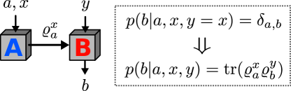
The idea of our certification scheme is very intuitive, yet powerful (see Fig. 1). Assume that Alice and Bob prepared their devices in a way that , whenever and . In other words, outcomes of Bob’s measurement are perfectly correlated with the preparations of Alice (whenever ). Since we assumed the upper bound of on the Hilbert space’s dimension in which experimental states and measurements are defined, and in this space, we have a set of quantum states and a POVM with effects which produce perfect correlations, we can conclude that, first, the Hilbert space’s dimension must be exactly , and second that , for all and . Clearly, after these perfect correlations are established, the “cross-terms”, can be used to compute the overlaps between the preparation states and between measurement operators: . Therefore, if the experimental statistics match the target statistics , we can certify that overlaps between experimental states match those of the target states. The same holds for the corresponding measurement operators.
Our method can be also applied when experimental statistics do not match exactly the target ones.
Theorem 1 (Robust SDI certification of overlaps).
Consider pure target qudit preparation states and target projective measurements , where and . Assume that for all and furthermore that experimental states and measurements act on Hilbert space of dimension at most and generate statistics such that , for all . Then, input states are almost pure and measurements are almost projective in the sense that
| (1) | |||
| (2) |
Moreover, for all , , , and , we have
| (3) | |||
The parameter accounts for all possible experimental errors, including the finite statistics’ error that can be estimated using standard tools of statistical analysis.
Proof.
We start with a straightforward proof of Eq.(2). Since for any state , the relation , valid for all , implies , for all , and hence for all we have .
To prove the bounds on the norms of experimental states in Eq. (1), we fix a setting and use a decomposition:
| (4) |
where is the largest eigenvalue of , is the corresponding eigenvector and, is a positive-semi-definite operator satisfying (to keep the derivations legible, we omit the index ). Using the fact that observed statistics are close to the target ones we get:
| (5) |
By taking the sum over we obtain . We can now use the identity , which follows form that fact that operators form a POVM in . This equality allows us to give a bound:
| (6) |
which is equivalent to . Inserting this to we obtain Eq. (1).
We now proceed to the proof of Eqs. (3). We start with the one for the overlaps between preparation states. The proof is given by the following sequence of inequalities which hold for every , :
All of the above inequalities are pretty straightforward apart from that we prove below. For this we again use the partial spectral decomposition form Eq. (4) (without writing the superscript as above) which implies:
| (7) |
The proof for the overlaps of POVM effects is very similar to the one for states with the only difference being the following inequality:
| (8) |
that is used in the second step in the proof in Eq. (3). One can easily verify the validity of this inequality by writing once more the decomposition and remembering that . ∎
The above result states that if the statistics observed in our certification scheme vary just a little bit form the target ones, the overlaps of the experimental states are also close to the overlaps between target states (and analogously for measurements). To our best knowledge analogous results have been previously known only for very special symmetric target states and measurements forming MUBs [23, 24].
4 Self-testing of qubits
We now show that certification of overlaps allows to prove robust self-testing result for arbitrary pure qubit preparations and projective measurements appearing in our certification scheme.
Theorem 2 (Robust self-testing of qubit systems).
Consider target pure qubit states and projective measurements , where , , and for all . Assume that experimental qubit states and measurements generate statistics such that , for all and . Then, there exist such that for there exist a qubit unitary such that
| (9) |
where is a potential transposition with respect to a fixed basis in that may have to be applied to all experimental states and measurements at the same time. Moreover, functions depend solely on the target states and measurements and, for small , have the asymptotics .
In the above we used the fidelity to indicate the closeness between rotated experimental states and target pure states (and analogously for measurements), following existing literature. The case corresponds to ideal reconstruction of target states and measurements after applying a suitable isometry. We remark that we allow only unitary operations (and possible transposition), as opposed to general channels [23, 26], to be applied to the experimental states in order to approximate the target states as well as possible.
In Appendix B we give a formal version of the above result and its proof. Moreover, we present there robustness bounds expressed in terms of the trace distance and its analogue for measurements [33]. We remark that the functions become unbounded once Bloch vectors of target qubit states become singular, i.e., once the target states are close to being aligned in a space of smaller dimension.
Remark.
Sketch of the proof.
We give a full proof for the ideal case () below. From Theorem 1 it follows that for all we have and . Using the Bloch representation, , we can conclude that also , where and are Bloch vectors of and respectively.
Assume now that the vectors are linear independent. Let be the linear transformation defined by , , and let be the matrix whose rows are the vectors , . Then, we have , and consequently, since is invertible by the construction, , i.e., is an orthogonal transformation in . It is well-known [36] that if , there exist a unitary matrix such that for and . By our assumption all remaining states can be decomposed in the basis , with the coefficients depending solely on the overlaps . The, the same that maps to , for , also connects the remaining pairs of states. Finally, if , the transformation corresponds to application of the transposition in the standard basis of followed by application of a unitary operation , determined by [37].
For the general case we consider Cholesky factorisations of Gram matrices, denoted by and , of Bloch vectors and their experimental counterparts respectively. Theorem 1 is then used to bound and utilize results of Ref. [38] to gauge how much the Cholesky decompositions of and differ in the Frobenius norm. The latter can be connected to the average fidelity between the selected target and experimental states. The robustness for the remaining states follows from the fact that they can be decomposed (as operators) using the three initially chosen target states and the identity.
If vectors from the set span two dimensional space then the same arguments for both and can be repeated for the considered subspace. Importantly, in this case additional transposition is not necessary. ∎
5 Examples
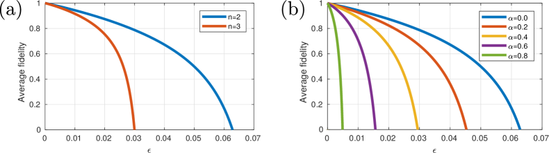
We now apply the quantitative formulation of Theorem 2 to lower-bound average fidelities for different configurations of target states as a function of the allowed error . In Figure 2 we present results for eigenstates of and Pauli matrices (i.e., states forming and qubit MUBs), and states belonging to two biased projective measurements satisfying , where we take .
For MUBs we compare our results with Ref. [23] that focuses on self-testing of qubit MUBs. The results of Ref. [23] give the upper bound on average fidelity equal for the deviation of in the figure of merit. In our scheme this happens for as shown on Fig. 2. To test the versatility of our scheme, we also applied it to MUBs, trine and tetrahedral configurations of qubit states. Quantitative results concerning these examples are listed in Table 1, while detailed derivations are given in Appendix D. For trine and tetrahedral configurations the robustness is obtained via the so-called Procrustes problem, described in Appendix C, based on Ref. [39]. For cases other than two MUBs we cannot make any comparison with the existing literature since, to our best knowledge, these case have not been studied previously.
| Configuration | ||
|---|---|---|
| 2 MUBs | ||
| 3 MUBs | ||
| 2 biased bases | ||
| Trine | ||
| Tetrahedron |
6 Shared randomness
Throughout the article we assumed that preparation and measurement devices are uncorrelated, which is often true in practice. However, one may also consider a situation in which Alice and Bob share a random variable , that they can use to coordinate their actions in a given round of the experiment. The most general statistics that can be generated in such a scenario can be expressed as , where denotes the probability distribution of .
Interestingly, the presence of shared randomness makes our main results, as stated by Theorems 1 and 2, inapplicable. The easiest way to see it is to consider the following simple example of , one bit of shared randomness , and , . This clearly satisfies the requirement on . Now, Alice’s and Bob’s devices can decide to “flip" their preparations and measurement operators whenever , and (note that can be distributed in an arbitrary way). This procedure does not affect the correlations , but it can be used to set to an arbitrary value.
Additionally, we believe that in the presence of shared randomness, the usual notion of self-testing in the SDI setting has to be reconsidered. Specifically, for any quantum realisation giving the statistics , one can always consider a strategy in which with probability Alice prepares states and Bob implements measurements , where is some arbitrary unitary transformation depending on . Clearly, such strategy reproduces the original statistics, and makes it impossible to find a single unitary that connects the target and experimental states (or measurements).
A very similar argument as above can be applied to situations of non-identical preparations of states and non-identical measurements across different runs of the experiment. Indeed, the value of a given run of the experiment is accessible to both Alice and Bob and can be considered a shared random variable that controls both Alice’s and Bob’s devices. Once again, the existence of a single unitary that connects the target and experimental states can never be guaranteed.
While, we do not consider the assumption on no shared randomness strong, below we propose a modification of our SDI certification scheme that allows to certify overlaps between arbitrary pure states even in the presence of shared randomness. The idea is to introduce, for every pair of non-orthogonal states, a suitable intermediate state [40], that enforces fixed overlaps between experimental states in every round of the experiment.
Recall that in our certification scheme we consider pure target qudit states and target projective measurements , where and . We extend this scheme by introducing an additional intermediate target state for every two pairs of Alice’s input , , where and . The state is chosen as the unique state satisfying:
| (10) |
Let denote the experimental statistics, corresponding to inputs and outcome . In the ideal scenario, in which experimental statistics satisfy assumptions of Theorem 1 with , assume additionally that Below we prove that under the above assumptions for all we have . Since in the ideal case overlaps between preparation states do not depend on and match the target value, our modified certification scheme works also in the presence of shared randomness. In the noisy scenario one can generally expect to be able to upper-bound the probability (over the choice of ) of the deviations from perfect correlations between states and measurements, as a function of the error . We postpone the discussion of this interesting point to the future work.
Proof of soundness of certification in the presence of shared randomness.
Consider a general physical realisation of experimental statistics , via classically correlated preparations and measurements on :
| (11) | ||||
| (12) |
where , and the variable (input) labels elements in the set of unordered pairs , where and . Assume now that the above statistics match exactly the ones required by our scheme and are compatible with Eq. (10) in the sense that:
| (13) | |||||
| (14) |
In what follows we prove that if the above constraints are satisfied, then for all111Technically speaking this equality holds for almost all .:
| (15) | |||||
| (16) |
where , . The above equation means that the overlaps between preparation sates (and measurements) do not depend on on the value of the shared random variable .
The proof of Eq. (15) is straightforward. Namely, form Eq. (13) if follows that:
| (17) |
Since , we get that for all we have . Since this reasoning can be repeated for all (for the fixed value of ) and since operators form a POVM on , we finally get Eq. (15).
The proof of Eq. (16) is more involved and relies on both Eqs. (13) and (14). Specifically, from Eq. (13) and the already established identity , it follows that Eq. (14) is equivalent to:
| (18) |
where moreover:
| (19) |
Using Bloch representation of qubit states (states are pure and hence span a two dimensional subspace of ) it is straightforward to obtain the bound:
| (20) |
After setting and using Eq. (19) we obtain:
| (21) |
Using Chauchy-Schwartz inequality for the left hand side of the above inequality we finally get:
| (22) |
which is equivalent to saying that the variance of the random variable vanishes. Therefore, , where is some numerical constant. We conclude the proof by noting that from Eq. (19) it follows that which implies Eq. (16). ∎
7 Extension of the scheme to SDI characterization of rank-1 non-projective measurements
In our work we focus on self-testing of arbitrary configurations of preparation states and projective measurements. In this section we discuss possible extension of our results to certification of properties of general rank-1 measurements in arbitrary dimension . To that end, we introduce additional states coming from suitably-chosen orthonormal bases per every effect of the measurement we want to certify. With the help of these extra states (and corresponding projective measurements) we can e.g., certify the following properties of POVMs in arbitrary dimension : (i) information completeness, (ii) extremality of rank-1 POVMs, and (iii) SIC-property.
The main idea of the extension is the following. Suppose we would like to self-test an -outcome POVM acting on a Hilbert space of dimension with each effect being of rank i.e., , for some pure states and positive scalars . We consider sets of preparation states , , and the corresponding projective measurements , . Assume now that in the idealized case we observe statistics satisfying:
| (23) |
From the second set of conditions we conclude that forms, as before, a basis of pure states for each . From the first condition in Eq. (7) we get that has to be a rank-1 POVM and, moreover, that ( is orthogonal to all of the states except the one with ). Consequently, we have for all . This fact together with the measured overlaps gives the information about the overlaps between effects of the POVM .
The knowledge of all overlaps (including ) and the fact that is a rank-1 POVM allow to certify many interesting properties of . First, as long as we can certify extremality of . This follows from the fact that rank-1 POVMs are extremal if and only if their effects are linearly independent (see e.g., Ref. [41]). Linear independence can be directly inferred from the experimentally accessible moment matrix . Specifically, is non-singular if and only if operators are linear independent. Now, if we can use the same reasoning to infer information completeness of . Finally, from the moment matrix we can directly verify the SIC property i.e., the condition .
8 Discussion
We have presented a systematic analytical scheme for noise-resilient certification of overlaps between arbitrary configurations of pure quantum states and rank- projective measurements in the prepare-and-measure scenario. For qubits our scheme can be used to robustly self-test general ensembles of pure quantum sates and the corresponding projective measurements. We believe that these findings pave the way towards systematic certification of general quantum systems in the semi-device-independent paradigm. This is supported by the concrete qubit results from Table 1 and by the universality of our protocol for certifying overlaps of quantum sates in arbitrary dimension.
In our main claims, we state that the scheme can be applied to an arbitrary set of preparation states. However, the sets of states in Theorems 1 and 2 always come in a collection of bases. These two statements are not contradicting one another since any given constellation of states can always be completed to a set of bases by adding extra preparation states. In practice, one should aim at aligning each basis of preparation states and the corresponding measurement to the best degree allowed by the experimental setup.
There are many exciting research directions that stem from our work. One of them is a systematic SDI characterization of generalized measurements beyond qubits. Another research direction is the robustness analysis of our scheme in the presence of shared randomness. An important contribution to the field of self-testing would be a generalization of our self-testing results for qubit to higher-dimensional systems. Finally, it is interesting to combine our methods with recent findings relating state discrimination games and resource theories of measurements and channels [42, 43, 44].
We would also like to draw reader’s attention to a related work [45].
Acknowledgements
We thank Marcin Pawłowski, Jedrzej Kaniewski and Tanmoy Biswas for interesting discussions and comments. NM acknowledges the financial support by First TEAM Grant No. 2016-1/5. We acknowledge partial support by the Foundation for Polish Science (IRAP project, ICTQT, contract no. 2018/MAB/5, co-financed by EU within Smart Growth Operational Programme). We acknowledge the support from International Research Agendas Programme of the Foundation for Polish Science funded by the European Regional Development Fund. MO acknowledges the financial support by TEAM-NET project (contract no. POIR.04.04.00-00-17C1/18-00).
Appendix
In this Appendix we provide technical details that were omitted in the main text. First, in Appendix A we prove statements regarding saturation of the bounds in Theorem 1. Second, in Appendix B we formulate and prove a quantitative version of Theorem 2, which concerns robustness of our self-testing protocol expressed in terms of average fidelities. We also prove there Theorem 3 that gives analogous results expressed in terms of trace distance. In Appendix C we provide alternative robustness analysis based on orthogonal Procrustes problem. In Appendix D we provide technical details about the considered examples in Table 1. Finally, in Appendix E we give proofs of two auxiliary Lemmas needed in the proof of the technical version of Theorem 2.
Appendix A Explicit form of states and measurements saturating the bounds in Theorem 1
We start by giving an example of four states and two qubit measurements (, ), for which the bound in Eq. (3) on the deviation of the overlaps scales like . Their explicit form is given below:
| (24) |
where , and as required by our scheme and , for all . Let the experimental states and measurements be the following:
| (25) |
First, we need to show that the experimental statistics is deviated from the target one by at most , i.e., . Since for both , it is sufficient to consider the cases of . Calculating the statistics we can see that , and and the latter is just the same as the target probability, . Finally, calculation of the overlap between the states yields:
| (26) |
which confirms the scaling of the first order of .
Now, let us show that the bounds from Eq. (3) are also tight in the first order of . We still consider the case of , but now is arbitrary. Let us consider the following POVM:
| (27) |
where , is the computational basis of and is the "maximally coherent" state in the subspace spanned by . In the proof of Theorem 1 the quantity is upper-bounded by , for which there exist a state and an effect reaching the bound. Now if we take to be the POVM we just introduced, and , , , the conditions of the Theorem 1 will be satisfied and the resulting bound will be .
Appendix B Quantitative statement of the robust self-testing
In this part we first formulate Theorem 3 in which we present robustness of our self-testing scheme in terms of trace distance222Recall that the trace distance is defined via and it has a neat operational interpretation in term of optimal success probability of distinguishing and via the most general quantum measurements: . for states and operator norm for measurements. Then, we give a quantitative statement of Theorem 2, that concerns robustness of our self-testing scheme in terms of average fidelities. We then proceed with proofs of both results.
In what follows we will need the following definition.
Definition 1.
Let be a set of vectors in . Matrix is called the Gram matrix of the set , if its elements are given by , .
Theorem 3 (Robust self-testing for qubits via trace distance and operator norm).
Consider pure target qubit preparation states and target projective measurements , where and . Assume that for all and, furthermore, that experimental states and measurements act on Hilbert space of dimension at most and generate statistics such that , for all .
Let be the cardinality of the maximal set of linearly independent Bloch vectors of states . Fix a set of linearly independent vectors , construct their Gram matrix , and let be a Cholesky factor of (i.e., and is lower triangular). For every and both let , denote the coefficients of decomposition of as a linear combination of . Finally, let us define three auxiliary functions
| (28) | |||
Then, there is a region of determined by
| (29) |
for which there exist a qubit unitary matrix such that
| (30a) | ||||
| (30b) | ||||
| (30c) | ||||
| (30d) | ||||
| (30e) | ||||
where is the transposition (with respect a fixed basis in ) that may have to be applied to all experimental states and measurements simultaneously.
The reason for such a formulation of the theorem lays in the proof techniques that were used to derive it. Namely, we use results on the stability of the Cholesky factorization. Since the result employed by us (Ref. [38]) is valid for positive-definite matrices we cannot apply it to the Gram matrix of all of the vectors due to their linear dependence. As a result, our bounds depend on the particular choice of the set of states whose Bloch vectors are linearly independent. In what follows, without the loss of generality we take for and for in the proof. In practice, however, one should consider all subsets of states that give non-singular Gram matrices having in mind a specific application.
Outline of the proof.– In what follows we will consider a particular subset of linearly independent Bloch vectors. For simplify we will omit the subscript whenever possible. The main idea of the proof is to use a Cholesky factors of the Gram matrices and of target () and experimental () Bloch vectors respectively. We then make use of the result of Ref. [38] on the stability of Cholesky factorization which, in simple terms, states that if and are close to each other, so are their Cholesky factors and . Specifically, this result, which we quote bellow (see Theorem [Sun 1991]), sets an upper bound on the Frobenius norm of in terms of the Frobenius norm of the perturbation . The Frobeniuous norm of the perturbation can be connected to the trace distance between states and the rotated states in the selected subset . On the other hand, the bound on can be estimated from our assumption: . This bound follows directly from the results of Theorem 1, but here we use an improved qubit stability bounds, which are given by Lemma 1. This, in turn, leads to stronger estimates for the norms of in Lemma 2 bellow. Combining all these results produces bounds in Eq. (30a).
In the next part of the proof we determine the trace distance between states and for based solely on the fact that and are close to . This gives the bounds in Eq. (30b). For states we use the fact that they can be decomposed in the basis of the states in . Since this linear decomposition can be different for target and experimental states, we use the result on stability of linear systems (see Theorem [Higham 2002], which we also quote below). The bounds for the states are given by Eq. (30c). Finally, we connect the bounds for the distance between the target and experimental measurements and the distance between the corresponding states resulting in Eq. (30d) and (30e).
Theorem 2 (Quantitative formulation of robust self-testing for qubits).
Consider pure target qubit preparation states and target projective measurements , where and . Assume that for all and, furthermore, that experimental states and measurements act on Hilbert space of dimension at most and generate statistics such that , for all .
Let be the cardinality of the maximal set of linearly independent Bloch vectors of states . Fix a set of linearly independent vectors , construct their Gram matrix , and let be a Cholesky factor of (i.e., and is lower triangular). For every and both let , denote the coefficients of decomposition of as a linear combination of . Finally, let us define three auxiliary functions
| (31) |
Then, there is a region of determined by
| (32) |
for which there exist a qubit unitary matrix such that
| (33a) | ||||
| (33b) | ||||
| (33c) | ||||
| (33d) | ||||
| (33e) | ||||
where is the transposition (with respect a fixed basis in ) that may have to be applied to all experimental states and measurements simultaneously. Note that in formulas (33c) and (30e) we have used trace distance in order to simplify the resulting formulas. The bound on this quantity is given in Eq. (30c).
Remark.
Results of Theorem 2 are obtained using a similar reasoning to that given in the outline of the proof of Theorem 3. However, the proof steps are supplemented by bounds connecting fidelity to the trace distance (for states) and operator norm (for measurement operators). The proof of Theorem 2 is given at the end of this part of the Appendix.
Before we proceed we state two theorems from the literature that are needed for our proof. First, we repeat the statement of the Theorem 1.4 from Ref. [38] for real-valued matrices. Second, we state a result concerning stability of systems of linear equation, which we borrow from Ref. [46] (Theorem 7.2). We changed the notation used in these papers in accordance with our paper.
Theorem (Sun 1991 - Stability of Cholesky factorisation).
Let be an positive definite matrix and its Cholesky factorization. If is an symmetric matrix satisfying
| (34) |
then there is a unique Cholesky factorization
and
| (35) |
Remark.
Theorem (Higham 2002 - Stability of systems of linear equations).
Let be a solution of a system of linear equations , where and . Let now be a solution to , where , . Assume that there exits such that and (for some , ), and that . Then, we have
| (36) |
Lemma 1.
Under the conditions of Theorem 1 qubit states and measurements , and , satisfy
and respectively, and .
Lemma 2.
Let be the Gram matrix of Bloch vectors of target states . Likewise, let be the Gram matrix of Bloch vectors of experimental states . Let for all and let be the cardinality of the set . Then, we have the following bounds on norms of
| (37) |
where
Proof of Theorem 3.
Let be the Gram matrix of Bloch vectors of the experimental states for . Let us for now assume that the Cholesky factorization exists and let .
We start our first part of the proof regarding the states , by connecting the square of the norm with trace distance between the states and . From the sketch of the proof of Theorem 3 it follows that the Bloch vectors of the target states and the vectors , transpose of which are rows of , are connected via an orthogonal transformation, which we denote as , i.e., , . Similarly, for the Bloch vectors of the experimental states and the vectors that form there exists an orthogonal transformation , such that , . Let us define states , and , . We know that there exist unitary transformations and such that: , and for (the optional transposition is reserved for the cases and ). We have the following sequence of equalities valid for :
| (38) | |||||
where we used the invariance of trace distancee under unitary evolution and transposition, and also denoted the resulting unitary as . It is clear that one transposition in the final formula in Eq. (38) is enough as the case is equivalent to having and changing to .
We need to show now that this unitary satisfies the claim of Theorem 2 for the states . For qubits, trace distance can be expressed directly via Eucleedian distance between Bloch vectors:
| (39) |
Using this fact and Eq. (38), it is straightforward to derive the following upper bound:
| (40) |
We now use Theorem [Sun 1991] (Ref. [38]) to upper-bound . Specifically, we apply it to the Gram matrix of the Bloch vectors of states . We have , since the target states are assumed to be pure. The direct substitution of the bound in Eq. (35) into Eq. (40) gives the bound in Eq. (30a), and also the condition in Eq. (29) when the Theorem 3 (and also Theorem 2) applies.
In the beginning of the proof we assumed that the Cholesky factorization exists. The condition in Eq. (29) gives the sufficient condition for this to hold. We conclude this part of the proof by noting that a similar statement in terms of fidelity (Theorem 2, Eq. (33a)) follows from Eq. (40) by connecting fidelity to the trace distance as described in Eq. (54).
In the second part of the proof we derive upper bounds on the trace distances between the states corresponding to and . As we will see, those can be connected to the bounds for the states with and . Indeed, we can write the following for every :
Exactly the same reasoning can be applied to upper bound the trace distance , in which case the transposition will propagate to but would not affect the term (as we can take ).
To finish the calculations we need to upper-bound the second summand in Eq. (B). We do it by writing , , where the last inequality is proven in Lemma 1 (see Eq. (77)). From here, it is easy to obtain the bound in Eq. (30b). The reason why we do not simply apply the same reasoning to the states corresponding to and as for the states with is because we want the isometry to be the same for all of the states.
In the third part of the proof we derive the bounds for the preparations states corresponding to and both . We start by reminding ourselves that the set of states is assumed to be tomographically complete. Is is equivalent to the assumption that the vectors , defined above, are linearly independent and span for , or the considered subspace for . The condition in Eq. (29) of the Theorem 3 (also stated in Eq. (34)) ensures that the same holds for the vectors . If so, let us expand the Bloch vectors of the states and , in terms of and respectively. Let us denote the coefficients of these linear expansions as and respectively. These coefficients will, of course, depend on and as well as on the choice of the set . However, for simplicity of the derivations we are going omit the subscripts and until we present the final result. We will also assume, without loss of generality, that (or for ).
It is clear that the coefficients and satisfy the following respective systems of linear equations:
| (42) |
where , and analogously , whenever the cardinality of the set is . For and their definition is analogous. We again omitted the subscripts for the vectors and for simplicity. The matrices and are still the moment matrices for the states , .
In complete analogy to Eq. (39) we can write:
| (43) |
We then can upper-bound the latter norm as follows:
In the equation above we used the following relation:
| (45) |
Also, since the norms can be upper-bounded by for all , the resulting upper bound can be simplified further to be .
To estimate the deviation we apply Theorem [Higham 2002] by taking and . The bound on the operator norm is given by Lemma 2. At the same time . If we take , some matrix with , vector such that , we satisfy the conditions of the Theorem [Higham 2002] and get the following bound:
| (46) |
As the final step we need to connect the bound in Eq. (B) with the one in Eq. (46) by the relation between -norm and the Euclidean norm in , which effectively adds a factor of to the bound in Eq. (46). Combining everything together we obtain the following:
| (47) |
The above bound is given in Eq. (30c) in terms of the quantity (Eq. (28)), where we took and brought back all the necessary subscripts. Again, using the relation in Eq. (55) we can derive bounds on the fidelity between the states and for .
In the fourth, final, part of the proof we derive the bounds for the measurements. We do it by connecting the distance between the experimental measurements and the distance between the corresponding states. Indeed, we can write the following:
| (48) |
where we used the triangle inequality and the invariance of the norm under unitary transformations. Remembering that (Lemma 1, Eq. (77)) and , we produce the bounds in Eqs. (30d,30e). ∎
Finally, we proceed to the proof of Theorem 2, which gives a quantitative robustness analysis expressed in terms of average fidelity.
Proof of Theorem 2.
Let us first state a useful identity between Frobenius distance and the fidelity, valid for an arbitrary pure states and a Hermitian operator :
| (49) |
We follow exactly the same steps that were given in the proof of Theorem 3. We assume that the reader is familiar with the notation introduced there. First, in order to derive the bound in Eq. (33a) we repeat the reasoning preceding Eq. (38). Analogously to the trace distance discussed there, we use the invariance of the fidelity under unitary transformations and transposition which gives us for all :
| (50) |
where . Using the above formula and standard algebra involving Pauli matrices we obtain:
| (51) |
On the other hand, we have the following identity:
| (52) |
where is a standard Euclidean norm in . Using the identity and the fact that target states are pure (which implies ) we obtain:
| (53) |
Inserting the above into Eq. (51) and using the fact that (this follows straightforwardly from Lemma 2), we finally obtain:
| (54) |
We complete the proof of Eq. (33a) by again employing, exactly as before, Theorem [Sun 1991] (Ref. [38]) in order to upper-bound .
Now, to derive Eq. (33b), which gives the bounds for the fidelity of states for and , we can use the following inequality which can be derived from Eq. (49) and from the relation :
| (55) |
From Eqs. (40,B) it follows that:
| (56) | |||
which gives the desired bound form Eq. (33b):
| (57) |
The proof of the remaining bounds in Eqs. (33c,33d,33e) is straightforward and follows directly form the formula in Eq. (49). In particular, in order to prove Eq. (33c) we set and in Eq. (49), use the inequality and the relation , with latter being true for arbitrary qubits states and . Derivation of Eq. (33d) is completely analogous to the one of Eq. (33b). Finally, for Eq. (33e), the reasoning is again analogous to Eq. (33c), where, after setting and , it is additionally necessary to use a simple lower bound: , which follows from the conditions of Theorem 2. ∎
Appendix C Alternative bounds from Procrustes
Lemma 3 (Robust self-testing for qubits from Procrustes).
Consider pure target qubit preparation states and target projective measurements , where and . Assume that for all and, furthermore, that experimental states and measurements act on Hilbert space of dimension at most and generate statistics such that , for all .
Let be a subset of considered states among . Let be a matrix whose rows are the Bloch vectors of states , , and let be its rank (). Assume, without loss of generality, that for the third component of the Bloch vectors is . In that case, truncate to the first two columns. Let us define two auxiliary functions:
| (58) |
and
| (59) |
where . There exist a unitary matrix such that:
| (60) |
In this section we derive alternative bounds for the fidelity between preparation states that follows from the bounds on the so-called orthogonal Procrustes problem [48]. The problem itself can be formulated as follows. Given two sets of vectors and in find an orthogonal transformation in that minimizes . This problem has a clear relevance to our task. Indeed, if we take to be the Bloch vectors of the target qubit preparation states and the Bloch vectors of the experimental states, then minimization over is the same as the problem of finding a unitary transformation that connects those qubit states. In Ref. [39] the bounds on Procrustes problem were derived. We give formulation of Theorem 1 from Ref. [39] below, where we change the notation according to our problem.
Theorem (Arias-Castro et.al. 2020 - A perturbation bound for Procrustes).
Given two tall matrices and of same size with having full rank, and set . Then we have
| (61) |
In the formulation of the above theorem stands for the Moore–Penrose inverse, which can be defined as for tall matrices of full rank.
Proof of Lemma 3.
. Unitizing the results of the Theorem [Arias-Castro et.al. 2020] is rather straightforward. Let be a matrix which rows are the Bloch vectors of all target preparation states . Let in turn be the matrix of Bloch vectors of the experimental states . The matrices and are then, of course, the full Gram matrices and . By “full" we mean that now we do not select a subset of linearly independent vectors among the Bloch vectors of . Instead, and are formed by all the considered states, which can still be a subset of the states (, ). We will be using to denote the number of the considered states, and a simple one-indexed set to denote the states themselves. Estimating from the formulation of the Theorem [Arias-Castro et.al. 2020] is a direct application of the bound on from Lemma 2, where now instead of one should put the number of the considered preparation states.
As for the left-hand side of Eq. (61), we can write the following:
| (62) |
where we use the following identity:
| (63) |
and is the unitary transformation in corresponding to the orthogonal transformation of the Bloch vectors. The bound on the average fidelity between target preparation states and the corresponding experimental states is then simply:
| (64) |
where
| (65) |
and
| (66) |
∎
Appendix D Examples
Below we provide detailed derivations of the results presented in Table 1.
The first example concerns MUBs in . Since for MUBs , for , it follows that is an identity matrix in (). Hence, in Theorem 2 (see Appendix B) we should take , and . The resulting bound is the average between expressions in Eq. (30a) and Eq. (30b) with the function being simply:
| (67) |
The leading linear term is given in Table 1 for both .
The second example is a little less straightforward. From the condition , we obtain that , and hence , , and . The output of the Cholesky factorization is , which leads to . This also determines the minimum in Eq. (28) to be . Plugging this values in Eq. (28) gives:
| (68) |
The final bound is again the average of the bounds in Eq. (30a) and Eq. (30b). The first order in for this bound is given in Table 1. The applicability of the above bound is determined by the inequality . Importantly, the latter condition gives nonempty region whenever .
The third example is a trine ensemble of states , with , , and where , , and . For this configuration of the preparation states the alternative robustness analysis via Procrustes (see Appendix C) gives better bounds. Given the vectors , we can directly compute that . Inserting this value to Lemma 3 produces the results given in Table 1.
The fourth example is the tetrahedron, with , , , , and , as before. In this case, we also employ the bounds from Procrustes. For the above configuration of states we have that , which leads to the results in Table 1.
Appendix E Proofs of auxiliary results
Proof of Lemma 1.
First of all, we improve the bound on the norm of each of the experimental states. From , for it follows immediately that the second (second largest) eigenvalue of each of the effects cannot exceed . Hence, we can conclude that .
Secondly, we can improve the bound on the norm of each of the experimental states. For that let us write the spectral decomposition of each experimental state and POVM effect:
| (69) | ||||
where we assume that . We omitted the indices for , and , for simplicity. We can assume, without loss of generality, that , and let us also assume for now that . From the condition , it then follows that:
| (70) |
from where we can obtain a lower bound on , namely:
| (71) |
The expression on the right-hand side of the above inequality is maximal when and , , which returns the bound .
Now let us return to our assumption , for which the above bound is valid. We can upper-bound by in Eq. (70), which returns nontrivial upper bound on that happens to be . This function is below for , i.e., for our newly-derived bound on is valid. The region is significantly larger than the resulting region in which our self-testing argument are valid, so this assumption does not affect our final results.
Let us now try to improve the bounds for the overlaps. In the proof of Theorem 1 (see Eq. (3)) we have already established that:
| (72) |
Let us now refine the bound on . For simplicity, we present this result below for a pair of operators and , that satisfy the conditions , and , . To compute the norm, we look for the eigenvector of the operator , i.e., , corresponding to the maximal eigenvalue. We have the following quadratic equation for the eigenvalue :
The sum of the roots of this equation is equal to . Since we know that , then either both roots are of the same sign, in which case the largest eigenvalue could only be , or they are of the opposite sign. In the latter case, it is evident that the absolute values of both roots are maximal whenever the free term in Eq. (E) is minimal. We then can upper-bound the solutions to Eq. (E) by lower-bounding the free term using the condition . Indeed, from we infer immediately that:
| (74) |
and thus we reduce Eq. (E) to:
| (75) |
Using the same argument we can set , because . The positive root of Eq. (75) is equal to:
| (76) |
It is easy to check that the above expression does not have any local maxima w.r.t. , on the domain , , whenever , which we assume to be the case. Thus, we conclude that the maximal value of corresponds to the boundary of the region of . By considering this boundary we find that this maximal value corresponds to the case of and which yields . From the above argument we finally conclude that:
| (77) |
which completes the proof for the state overlaps. From Eq. (77) and the fact that , it is easy to obtain the improved bound on the overlaps between measurement effect. ∎
Proof of Lemma 2.
Let us start by deriving the bound on the Frobenius norm :
| (78) |
We have already established the bound on in Lemma 1. The bound on can be obtained from the bound on the norm of each . Namely, from the condition we can immediately conclude that:
| (79) |
From here, it is easy to get to the final bound on , which reads:
| (80) |
where we made some approximations to simplify the result.
Now, let us derive the bound on . In principle, we know that , but we can derive a better bound based on the fact that the diagonal entries of are much less than the off-diagonal entries.
First of all, due to the triangle inequality, we can write , where we split on the diagonal and off-diagonal parts. The first term, , can be easily bounded as follows:
| (81) |
As for the off-diagonal part, we give the proof for two cases and separately. For , , where we used the results of Lemma 1. As for , we will need some intermediate result, namely the following relation:
| (82) |
where is the size of the matrix with . We give a proof of this below.
Let us assume that are the eigenvalues of matrix , hence we know that Let be the largest eigenvalue, i.e., the operator norm of , if . If we wish to maximize the Frobenius norm of for fixed , the following lower-bound has to be satisfied:
| (83) |
which proves the bound in Eq. (82). Using the above result, we obtain the following bound:
which completes out proof. ∎
References
- [1] F. Arute, K. Arya, R. Babbush, D. Bacon, J. C. Bardin, R. Barends, R. Biswas, S. Boixo, F. G. S. L. Brandao, D. A. Buell, B. Burkett, Y. Chen, Z. Chen, B. Chiaro, R. Collins, W. Courtney, A. Dunsworth, E. Farhi, B. Foxen, A. Fowler, C. Gidney, M. Giustina, R. Graff, K. Guerin, S. Habegger, M. P. Harrigan, M. J. Hartmann, A. Ho, M. Hoffmann, T. Huang, T. S. Humble, S. V. Isakov, E. Jeffrey, Z. Jiang, D. Kafri, K. Kechedzhi, J. Kelly, P. V. Klimov, S. Knysh, A. Korotkov, F. Kostritsa, D. Land huis, M. Lindmark, E. Lucero, D. Lyakh, S. Mandrà, J. R. McClean, M. McEwen, A. Megrant, X. Mi, K. Michielsen, M. Mohseni, J. Mutus, O. Naaman, M. Neeley, C. Neill, M. Y. Niu, E. Ostby, A. Petukhov, J. C. Platt, C. Quintana, E. G. Rieffel, P. Roushan, N. C. Rubin, D. Sank, K. J. Satzinger, V. Smelyanskiy, K. J. Sung, M. D. Trevithick, A. Vainsencher, B. Villalonga, T. White, Z. J. Yao, P. Yeh, A. Zalcman, H. Neven, and J. M. Martinis, Quantum supremacy using a programmable superconducting processor, Nature 574, 505 (2019).
- [2] C. L. Degen, F. Reinhard, and P. Cappellaro, Quantum sensing, Reviews of Modern Physics 89, 035002 (2017).
- [3] I. M. Georgescu, S. Ashhab, and F. Nori, Quantum simulation, Reviews of Modern Physics 86, 153 (2014).
- [4] A. Montanaro, Quantum algorithms: an overview, npj Quantum Information 2, 1 (2016).
- [5] J. Biamonte, P. Wittek, N. Pancotti, P. Rebentrost, N. Wiebe, and S. Lloyd, Quantum machine learning, Nature 549, 195 (2017).
- [6] V. Dunjko and H. J. Briegel, Machine learning & artificial intelligence in the quantum domain: a review of recent progress, Reports on Progress in Physics 81, 074001 (2018).
- [7] J. Eisert, D. Hangleiter, N. Walk, I. Roth, D. Markham, R. Parekh, U. Chabaud, and E. Kashefi, Quantum certification and benchmarking, Nature Reviews Physics 2, 382 (2020).
- [8] D. Mayers and A. Yao, Self testing quantum apparatus, arXiv preprint quant-ph/0307205 (2003).
- [9] I. Šupić and J. Bowles, Self-testing of quantum systems: a review, Quantum 4, 337 (2020).
- [10] J. S. Bell, On the Einstein Podolsky Rosen paradox, Physics Physique Fizika 1, 195 (1964).
- [11] S.-L. Chen, C. Budroni, Y.-C. Liang, and Y.-N. Chen, Natural framework for device-independent quantification of quantum steerability, measurement incompatibility, and self-testing, Physical Review Letters 116, 240401 (2016).
- [12] A. Coladangelo, K. T. Goh, and V. Scarani, All pure bipartite entangled states can be self-tested, Nature Communications 8, 15485 (2017).
- [13] J. Bowles, I. Šupić, D. Cavalcanti, and A. Acín, Device-independent entanglement certification of all entangled states, Physical Review Letters 121, 180503 (2018).
- [14] S. Popescu and D. Rohrlich, Which states violate Bell’s inequality maximally? Physics Letters A 169, 411 (1992).
- [15] J. Ahrens, P. Badziąg, M. Pawłowski, M. Żukowski, and M. Bourennane, Experimental tests of classical and quantum dimensionality, Physical Review Letters 112, 140401 (2014).
- [16] J. B. Brask, A. Martin, W. Esposito, R. Houlmann, J. Bowles, H. Zbinden, and N. Brunner, Megahertz-rate semi-device-independent quantum random number generators based on unambiguous state discrimination, Physical Review Applied 7, 054018 (2017).
- [17] E. A. Aguilar, M. Farkas, D. Martínez, M. Alvarado, J. Cariñe, G. B. Xavier, J. F. Barra, G. Cañas, M. Pawłowski, and G. Lima, Certifying an irreducible 1024-dimensional photonic state using refined dimension witnesses, Physical Review Letters 120, 230503 (2018).
- [18] H. Anwer, S. Muhammad, W. Cherifi, N. Miklin, A. Tavakoli, and M. Bourennane, Experimental characterization of unsharp qubit observables and sequential measurement incompatibility via quantum random access codes, Physical Review Letters 125, 080403 (2020).
- [19] M. Pawłowski and N. Brunner, Semi-device-independent security of one-way quantum key distribution, Physical Review A 84, 010302 (2011).
- [20] T. Van Himbeeck, E. Woodhead, N. J. Cerf, R. García-Patrón, and S. Pironio, Semi-device-independent framework based on natural physical assumptions, Quantum 1, 33 (2017).
- [21] R. Chaves, J. B. Brask, and N. Brunner, Device-independent tests of entropy, Physical Review Letters 115, 110501 (2015).
- [22] T. Fritz, Quantum correlations in the temporal Clauser–Horne–Shimony–Holt (CHSH) scenario, New Journal of Physics 12, 083055 (2010).
- [23] A. Tavakoli, J. Kaniewski, T. Vértesi, D. Rosset, and N. Brunner, Self-testing quantum states and measurements in the prepare-and-measure scenario, Physical Review A 98, 062307 (2018).
- [24] M. Farkas and J. Kaniewski, Self-testing mutually unbiased bases in the prepare-and-measure scenario, Physical Review A 99, 032316 (2019).
- [25] P. Mironowicz and M. Pawłowski, Experimentally feasible semi-device-independent certification of four-outcome positive-operator-valued measurements, Physical Review A 100, 030301 (2019).
- [26] A. Tavakoli, M. Smania, T. Vértesi, N. Brunner, and M. Bourennane, Self-testing non-projective quantum measurements, Science Advances 6, eaaw6664 (2020).
- [27] A. Tavakoli, D. Rosset, and M.-O. Renou, Enabling computation of correlation bounds for finite-dimensional quantum systems via symmetrization, Physical Review Letters 122, 070501 (2019).
- [28] R. Blume-Kohout, J. K. Gamble, E. Nielsen, K. Rudinger, J. Mizrahi, K. Fortier, and P. Maunz, Demonstration of qubit operations below a rigorous fault tolerance threshold with gate set tomography, Nature Communications 8, 1 (2017).
- [29] C. H. Bennett and G. Brassard, Quantum cryptography: Public-key distribution and coin tossing, Theoretical Computer Science 560, 7 (2014).
- [30] C. H. Bennett, Quantum cryptography using any two nonorthogonal states, Physical Review Letters 68, 3121 (1992).
- [31] E. Woodhead, C. C. W. Lim, and S. Pironio, Semi-device-independent QKD based on BB84 and a CHSH-type estimation, In Theory of Quantum Computation, Communication, and Cryptography, vol 7582, pages 107–115, Springer, Berlin, Heidelberg (2013).
- [32] J. I. de Vicente, Shared randomness and device-independent dimension witnessing, Physical Review A 95, 012340 (2017).
- [33] M. Navascués and S. Popescu, How energy conservation limits our measurements, Physical Review Letters 112, 140502 (2014).
- [34] J. M. Renes, R. Blume-Kohout, A. J. Scott, and C. M. Caves, Symmetric informationally complete quantum measurements, Journal of Mathematical Physics 45, 2171 (2004).
- [35] S. Brierley, S. Weigert, and I. Bengtsson, All mutually unbiased bases in dimensions two to five, arXiv preprint arXiv:0907.4097 (2009).
- [36] M. A. Nielsen and I. L. Chuang, Quantum Computation and Quantum Information: 10th Anniversary Edition, Cambridge University Press, USA, 10th edition (2011).
- [37] V. Bargmann, Note on Wigner’s theorem on symmetry operations, Journal of Mathematical Physics 5, 862 (1964).
- [38] J.-G. Sun, Perturbation bounds for the Cholesky and QR factorizations, BIT Numerical Mathematics 31, 341 (1991).
- [39] E. Arias-Castro, A. Javanmard, and B. Pelletier, Perturbation bounds for Procrustes, classical scaling, and trilateration, with applications to manifold learning, Journal of Machine Learning Research 21, 15 (2020).
- [40] H. Bechmann-Pasquinucci and N. Gisin, Intermediate states in quantum cryptography and Bell inequalities, Physical Review A 67, 062310 (2003).
- [41] G. M. D’Ariano, P. L. Presti, and P. Perinotti, Classical randomness in quantum measurements, Journal of Physics A: Mathematical and General 38, 5979 (2005).
- [42] M. Oszmaniec and T. Biswas, Operational relevance of resource theories of quantum measurements, Quantum 3, 133 (2019).
- [43] R. Takagi and B. Regula, General resource theories in quantum mechanics and beyond: operational characterization via discrimination tasks, Physical Review X 9, 031053 (2019).
- [44] R. Uola, T. Kraft, J. Shang, X.-D. Yu, and O. Gühne, Quantifying quantum resources with conic programming, Physical Review Letters 122, 130404 (2019).
- [45] A. Tavakoli, Semi-device-independent certification of independent quantum state and measurement devices, Physical Review Letters 125, 150503 (2020).
- [46] N. J. Higham, Accuracy and stability of numerical algorithms, Society for Industrial and Applied Mathematics, USA, 2nd edition (2002).
- [47] X.-W. Chang and D. Stehlé, Rigorous perturbation bounds of some matrix factorizations, SIAM Journal on Matrix Analysis and Applications 31, 2841 (2010).
- [48] J. R. Hurley and R. B. Cattell, The Procrustes program: Producing direct rotation to test a hypothesized factor structure, Behavioral Science 7, 258 (1962).