Identification of primary and collateral tracks in stuttered speech

Abstract

Disfluent speech has been previously addressed from two main perspectives: the clinical perspective focusing on diagnostic, and the Natural Language Processing (NLP) perspective aiming at modeling these events and detect them for downstream tasks. In addition, previous works often used different metrics depending on whether the input features are text or speech, making it difficult to compare the different contributions. Here, we introduce a new evaluation framework for disfluency detection inspired by the clinical and NLP perspective together with the theory of performance from [Clark, 1996] which distinguishes between primary and collateral tracks. We introduce a novel forced-aligned disfluency dataset from a corpus of semi-directed interviews, and present baseline results directly comparing the performance of text-based features (word and span information) and speech-based (acoustic-prosodic information). Finally, we introduce new audio features inspired by the word-based span features. We show experimentally that using these features outperformed the baselines for speech-based predictions on the present dataset.

Keywords: evaluation metrics, disfluency, stuttering, speech processing, audio features

1. Introduction

Around 6% percent of spoken words in non-pathological speech are categorised as disfluent [Tree, 1995] and this increases with the cognitive load of the speaker [Bortfeld et al., 2001, Lindström et al., 2008]. Speaking in real time is a demanding activity, subject to cognitive constraints and pragmatic settings. Under time pressure, a word may not be retrieved, part of a sentence may be revised, unfilled and filled pauses may be inserted, words or part of words may be repeated. Some of these deviations can be viewed as the symptoms of sentence planning problems [McRoberts and Clark, 1996] or as the results of some strategies [Clark and Wasow, 1998] unfolded under speaker’s control to signal something.

Stuttering is a severe case of speech pathology, that interrupts at a higher rate the flow of speech than in typical Speech Production. Indeed, in addition to the ’classic’ disfluencies, stutterers can produce other forms of disfluency that are both quantitatively and qualitatively distinguishable from typical forms [Lickley, 2017].

Speech pathologists need to quantify all the disfluency events for clinical screening but also to assess potential treatments [Yaruss, 1997]. A large number of factors and speaking settings influence stuttering behaviours and occurrences of disfluencies: interlocutor’s characteristics (ex: age, relationship with the speaker), conversational settings (at home, at the hospital, at work), speaking tasks (ex: reading, dialogues, descriptions of scenes). The clinical assessment still rely heavily on subjective and one on one evaluation [Yaruss and Quesal, 2006]. An automatic, reliable procedure would provide Speech Pathologists an objective comparison between clinical facilities and treatments. Besides, detecting automatically disfluencies and stuttering symptoms from speech, in different settings, could unlock in-home assessments and more frequent trainings for patients.

Two main issues arise from the literature around disfluency detection. The first one is the lack of public pathological annotated datasets. The second issue is the absence of a clear evaluation protocol for the automatic detection of disfluencies. This might be due to the fact that different communities have different applications in mind. Speech pathologists are interested in the automatic classification of type and duration of disfluencies [Yaruss, 1997]. Most used proprietary datasets, with patients performing reading tasks and where disfluent and non disfluent parts have been balanced [Nöth et al., 2000, Yildirim and Narayanan, 2009, Oue et al., 2015]. Researchers in the NLP community are interested in modelling the disfluencies for several reasons [Shriberg, 2001]: text normalisation for downstream tasks such as Dependency Parsing or Semantic Role Labeling. In addition, NLP researchers are also interested in disfluency detection for affective computing [Tian et al., 2015] applications. They use features derived from transcribed text [Honal and Schultz, 2003] using Shriberg’s formalism [Shriberg, 1994], and focus on the detection of disfluencies in non-pathological speech in telephonic conversation using datasets like Switchboard [Godfrey et al., 1992]. Yet, the work from [Goldwater et al., 2010] demonstrated that words preceding disfluent interruption points also have high error rates for speech recognition systems. Finally, psycholinguists and clinicians are interested in the distribution and type of disfluencies, which could inform on speech and language production systems [Jackson et al., 2015] [Fromkin, 1971] as well as diagnosis. Obviously, for this kind of application, running interview-like speech with minimal annotations would be preferable. Since several hybrid text/speech systems have been proposed [Tran et al., 2018, Yildirim and Narayanan, 2009], we believe that a common evaluation method would be beneficial to bridge the gap between these research communities.

First, we introduce a new framework for the evaluation of disfluency detection which would be relevant both for spontaneous and/or pathological speech using metrics combining insights from both NLP and Speech Technologies (ST) communities (Section 2). Second, we test these metrics on a new dataset obtained by force-aligning an annotated corpus of pathological speech (Section 3). All annotations in Praat format and code for evaluation will be released on the GitHub repository of the first author RR . Third, we compare the performance of different baseline systems across textual and speech inputs on this dataset that were usually used in NLP and ST (Section 4). Four, to bridge the gap in performance between NLP and ST methods, we introduce new audio features that improve on the different frame-based baselines (Section 5).

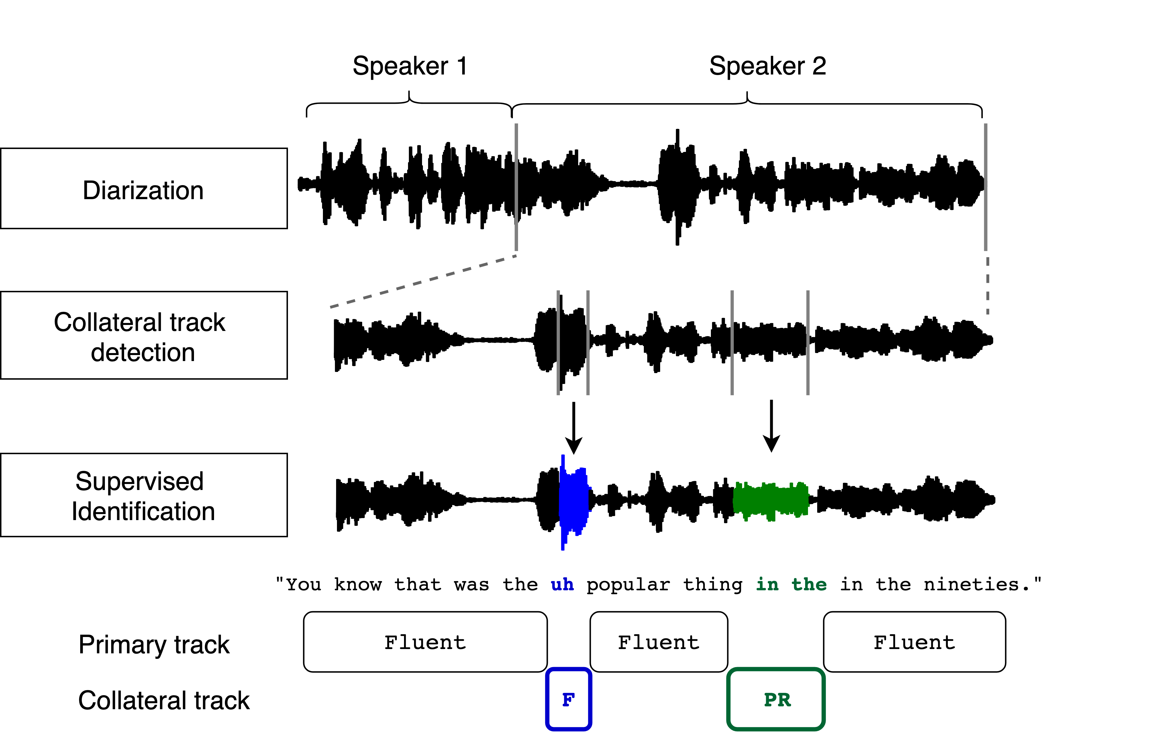
Figure 1: Schematic diagram of identification of the primary and collateral tracks of communication. In black the primary track (fluent), in other colors the words in the collateral track, in blue a filler, in green a phrase repetition.

2. Metrics: primary and collateral tracks

We take inspiration from the H. Clark’s theory of speech performance [Clark, 1996, p. 255], which states that speakers communicate using two parallel tracks. The primary track contains the traditional linguistic content of the discourse while the collateral track contains additional signals regulating the communication channel itself. Among these signals we find delays, (un)filled pauses, rephrasing, mistakes, laughs, or vocal noises. The extraction of these two tracks from continuous speech can be decomposed in several engineering tasks (see Figure 1). First, a diarization [Anguera et al., 2012] component involves assigning stretches of signal (turns) to each speaker. This component is well studied and existing evaluation metrics can be used (see [Bredin, 2017] for a suite of diagnostic tools). Second, each turn is analysed in terms which sub-part contains collateral information (collateral detection task). This allows us to quantify how well the collateral track (only disfluencies in this work) is detected without specifying their category. The parsed segments can be evaluated in terms of a gold lexicon and a gold alignment. For this, we report the Detection Error Rate and the Detection F1-score. Third, each collateral sub-part is categorised into a small number of categories, which we restrict here to disfluency types (identification task). For that purpose we use the Identification F1-score and the Identification Error Rate. The formula to obtain these metrics are summarised in the Table 1. The two error rate metrics are defined with the similar formula to that used in the Diarization Error Rate, which means that they can go over 100% (the denominator being restricted here to the collateral track). All these metrics were coded using the python toolkit $pyannote.metrics$ [Bredin, 2017].

Metrics	Formula
Detection Precision	$\frac{T_{\text{True Positive}}}{T_{\text{True Positive}}+T_{\text{false alarm}}}$
Detection Recall	$\frac{T_{\text{True Positive}}}{T_{\text{True Positive}}+T_{\text{missed detection}}}$
Detection F1-score	$2\frac{\text{detection precision}\times\text{detection recall}}{\text{detection precision}+\text{detection recall}}$
Detection Error Rate	$\frac{T_{\text{false alarm}}+T_{\text{missed detection}}}{T_{\text{Collateral Track}}}$
Identification Precision	$\frac{1}{5}\sum_{i}\text{Precision}_{i}$
Identification Recall	$\frac{1}{5}\sum_{i}\text{Recall}_{i}$
Identification F1-score	$2\frac{\text{identification precision}\times\text{identification recall}}{\text{identification precision}+\text{identification recall}}$
Identification Error Rate	$\frac{T_{\text{false alarm}}+T_{\text{missed detection}}+T_{\text{confusion}}}{T_{\text{Collateral Track}}}$

Table 1: Metrics used for the detection and identification of the collateral track. $T_{\text{false alarm}}$ is the duration of false alarm (e.g. primary track classified as collateral), $T_{\text{miss detection}}$ is the duration of missed detection (e.g. collateral track classified as primary), $T_{\text{Collateral Track}}$ is the total duration of the collateral track in the reference, $T_{\text{confusion}}$ is the total duration of the confusion between disfluency labels. Detection F1-score is computed as there are only two classes (primary and collateral). $\text{Precision}_{i}$ and $\text{Recall}_{i}$ are computed as the detection formula where the positive class is the i-th disfluency Table 2

Another motivation for this framework comes from speech pathology research on Stuttering evaluation. Indeed, from these timing prediction of the primary and collateral track, it can be computed automatically the Speech Efficiency Score (SES) introduced in [Amir et al., 2018]. This study demonstrated that this score, which is based on a time-domain analysis is closely equivalent to stuttering severity ratings done by speech pathologists. By solving the diarization task, and the disfluency detection task mentioned above, it is possible to obtain an estimation of the SES (see below the formula for the equivalence between our framework and their notations).

$$SES =\frac{T_{\text{Primary Track}}}{T_{\text{Primary Track}}+T_{\text{Collateral Track}}}*100$$

$$=\frac{T_{\text{Efficient time}}}{T_{\text{Total time}}-T_{\text{Silence}}}*100$$

3. Dataset

We built on FluencyBank, a large-scale open source audiovisual dataset primarily used by clinical researchers to study fluency [Bernstein and MacWhinney, 2018], from which we selected and forced-aligned a consistent subset focused on stuttering. FluencyBank contains a collection of sub-datasets collected by different research groups to study typical and disordered fluency in infants and adults. We selected the Adult-who-Stutter(AWS) sub-dataset of FluencyBank, which contains video recordings focused on patients. We excluded the recordings where the annotation was lacking, and we obtained 22 speaker video interviews (1429 utterances and 24693 words). The original recordings were done while the participants answered questions of the OASES elicitation protocol [Yaruss and Quesal, 2006], and transcriptions and disfluencies were done in the original dataset at the sentence level. Table 2 provides the five classes of disfluencies that we consider here. We provide some examples for each class of patients answering some questions of the protocol. In this work, we did not consider blocks, syllable repetitions or prolongations. Yet, our formulation with the primary and collateral tracks can easily be extended to these disfluencies.

We obtained the timings of the primary and collateral tracks by force-alignment at the phone level with the kaldi toolkit [Povey et al., 2011] with a HMM-GMM model. Figure 2 shows the distribution of disfluencies per speaker in the dataset. The total number of disfluencies and their types vary greatly across speakers.

Table 2: Collateral signals taxonomy (usually called disfluency) under consideration here in the FluencyBank dataset: Italic for the primary track and Bold for the collateral track.

Disfluency	Example
Filled pause (F)	I was primarily uh focused
	on fluency.
Single word Repetition (R)	I I don’t like switch word.
Multi-Repetition (MR)	I’m fortunate to be be be
	be in graduate school.
Phrase Repetition (PR)	they are they are so sweet.
Retracing or Revision (RT)	I ended when I was it ended
	when I was seventeen.

Figure 2: Distribution of disfluency in the FluencyBank-AWS per speaker. See table 2 for definitions of disfluencies.

4. Baselines: text versus speech predictions

Here, we provide two different kind of baseline systems with the purpose of comparing textual and acoustic approaches on the same metrics: (1) word-based systems, which assume that the input speech has been segmented into words, and aggregate textual and/or acoustic features over the entire span of each word (2), frame-based system which make decision on a frame-by frame basis from raw speech. Obviously, the latter kind of system cannot use textual features. All evaluations are performed with leave-one-speaker-out cross-validation, so that we can assess the generalisation to unseen speaker.

4.1. Detection from aligned speech: word-based systems

Word-based systems can incorporate both textual and acoustic features (See Table 3). As for textual features, we used token and span features which are common in the NLP community [Shriberg, 1994, Charniak and Johnson, 2001]. As for acoustic/prosodic, we use summary statistics on duration energy and F0. All statistics and pooling are done using the timing alignment of each word $w_{i}$. The semantic representation and part-of-speech tags are extracted with [Honnibal and Montani, 2017]. The number of syllables and phones are extracted with [Bernard et al., 2019].

Table 3: List of features in the word-based prediction.

Type	Core features and dimension
Token	semantic representation	384
	part-of-speech (pos): $p_{i}$	19
	word position	1
Span	$w_{i}==w_{i+k},k\in[-15,+15]^{*}$	30
	$p_{i}==p_{i+k},k\in[-15,+15]^{*}$	30
	$w_{i},w_{i+1}==w_{i+k},w_{i+k+1}$	8
	$k\in[-4,+4]^{*}$
	$p_{i},p_{i+1}==p_{i+k},p_{i+k+1}$	8
	$k\in[-4,+4]^{*}$
Acoustic	word duration (s)	1
Prosodic	number of syllables	1
	number of phones	1
	high, low and total energy	3
	in filterbanks
	F0 mean, std, median, min, max	9
	5%, 25%, 75% & 95% percentiles
	surrounding pause times (s)	2
	pitch breaks inside	3
	and around word limits

Such hand-crafted features have been used previously in the literature [Zayats et al., 2016, Ferguson et al., 2015] and have shown to improve the prediction performance. Indeed, neighbour words and prosodic cues are very informative about the disfluency events [Shriberg, 1994]. In [Yildirim and Narayanan, 2009], they obtained that interrupting points in disfluencies are 98% associated with a pitch break. We obtained a similar result in the FluencyBank AWS dataset with 95% of the disfluent boundaries that match with a pitch break in a 100 ms vicinity. All these features are normalized with the $MaxAbsScaler$ from scikit-learn [Pedregosa et al., 2011] to avoid the loss of sparsity (specially in the span features).

We compared 5 different models (see Table 4). The latest work is focusing on sequence tagging prediction with Recurrent Neural Network architectures [Zayats et al., 2016, Tran et al., 2018]. We compared Forward and Bi-Directional architectures with Long-Short-Term-Memory (LSTM) Networks for disfluency detection and identification. The hidden dimension of the recurrent networks is set at 20. All the experiments are carried using the Adam training procedure with the default parameters [Kingma and Ba, 2014] and early-stopping on a held-out validation set of 20% of spoken utterances of the training speakers. In addition, we used a discriminative approach with classical machine learning classifiers. Every word is supposed to be independent: the goal is now to predict each word individually, without its neighbour’s representation or prediction. The information listed in Table 3 is already obtained by the aggregation of local and long range information and could be sufficient to make predictions. We compare a standard classic Support Vector Machine with linear kernel (SVM) and a penalty term of $C=0.025$, a L2 regularised logistic regression and a classic deep forward neural network (DNN) with 2 hidden layers with 100 and 50 hidden units.

In the results, we also report the Token F1 score 4 at the word level to compare the predictions. This differs from the F1-score reported for disfluency detection in the NLP community [Godfrey et al., 1992]. Usually, NLP models tries to detect the disfluency and identify the subparts of each disfluency (reperandum, interegnum, repair), not the different categories of disfluencies.

4.2. Detection from raw speech: frame-based systems

Frame-based systems have no other information than speech. In principle, they are closer to what would be useful for clinical purposes, but obviously, the task is much harder. For comparison purposes we propose 3 baseline frame-based systems. Here, we evaluate frame-level prediction for the disfluency detection and identification as in [Oue et al., 2015]. The patterns of the disfluencies in the speech signal can range from very local phenomenon (filled pauses) to long time-scales (retracing). Here, we investigate the predictions are made every 10 ms, in a bottom-up manner, using only local features.

Speech represented using a bank of 40 log-energy Mel-scale filters representing 25 ms of speech (Hamming windowed) every 10 ms. The Mel features are mean-variance normalised per file, using the VAD information. Besides, we extract prosodic features with the F0 trajectory and its first derivatives in a 50 ms window (obtaining a 56-dimension vector as F0 is computed every 1.8ms). These spectral and prosodic representation are concatenated to obtain a final 106-dimension vector representation every 10 ms. All the frame-based systems use a window of 7 stacked frames [Oue et al., 2015].

Based on these representations directly extracted from the signal, we follow a similar procedure as in the word-based predictions: we compare a standard classic Support Vector Machine with linear kernel (SVM) and a penalty term of $C=0.025$, with a classic deep forward neural network (DNN) with 2 hidden layers with 100 and 50 hidden units. These approaches have been previously used in stuttering detection literature [Chee et al.,].

Table 4: Results of the evaluation of detection and identification of primary and collateral track for the different approaches described in Section 4. The best scores for each metric for each condition (word vs frame based) are in bold, best metrics overall are underlined. For the evaluation of the Audio Span Features, we report the performance with a DNN model trained with the Standard sampler.

Model	NLP	Detection				Identification
	Token F1	P	R	F1	Error Rate	P	R	F1	Error Rate
Word-based 4.1 (all features)
Forward LSTM	0.416	0.823	0.595	0.691	0.623	0.717	0.518	0.601	0.701
Bi-LSTM	0.417	0.786	0.605	0.684	0.731	0.701	0.537	0.608	0.799
SVM-Linear	0.569	0.966	0.642	0.771	0.381	0.905	0.599	0.721	0.424
Logistic Regression	0.544	0.846	0.645	0.732	0.513	0.762	0.576	0.656	0.581
DNN	0.485	0.958	0.611	0.746	0.417	0.855	0.544	0.665	0.484
Frame-based 4.2 (Baseline Signal features only)
Standard sampler + DNN	–	0.312	0.014	0.026	1.005	0.182	0.010	0.020	1.008
Undersampler + DNN	–	0.073	1.000	0.136	15.286	0.038	0.520	0.069	15.766
Standard sampler + SVM	–	0.150	0.086	0.109	1.502	0.116	0.067	0.086	1.520
Undersampler + SVM	–	0.077	0.838	0.140	12.529	0.025	0.288	0.048	13.079
Frame-based 5 (Audio Span Features)
Audio Span Features + Standard Sampler + DNN	–	0.864	$\leq 1\mathrm{e}{-3}$	$\leq 1\mathrm{e}{-3}$	1.000	0.818	$\leq 1\mathrm{e}{-3}$	$\leq 1\mathrm{e}{-3}$	1.003
Audio Span Features + baselines features + Standard Sampler + DNN	–	0.488	0.063	0.112	0.986	0.450	0.059	0.105	0.990

As in many machine learning problems [Lemaître et al., 2017], disfluency datasets have the attribute to be very imbalanced. The number of frames that are labelled fluent exceeds by a large margin all the others classes (92.7% of the frames are labelled as fluent). We evaluate a random undersampler technique [Lemaître et al., 2017] that discards randomly a large number of the majority class (here fluent) before training each model. This undersampling strategy has been used in Speech Technologies, yet, systems had not been evaluated on running speech datasets.

5. Audio Span Features

We want to improve the frame-based system using information over a long time span and replace the textual features with equivalent ones directly from the raw speech. We introduce here our Audio Span Features. The goal of these features is to obtain similar information as the span features from the word-based systems (Table 3).

Our main assumptions for disfluency events are: (1) Repetition-like disfluency events exhibit a common underlying structure property in the frequency domain, (2) filled pauses exhibit specific acoustic correlates with a steady frequency signature [Gabrea and O’Shaughnessy, 2000], (3) these filled pauses have usually adjacent unfilled pauses/silences [Daly, 1994].

That is why we posit that local neighbour-similarities in the frequency domain can approximate the span features for the word comparisons from Table 3. Besides, different chunk size can also inform on the different type of disfluencies (close and more local similarities are triggered by fillers versus spaced and long range similarities are triggered by repetitions of words).

Therefore, for every time-step $t$, for a given window-scale $s$, we compute the similarity $\psi(t,s,i)$ of the frequency representation $x_{t}$ centered on $t$ with its $i$-th closest neighbours. We compute this similarity with the $N$ previous neighbours and the $N$ next. The frequency representation $x_{t}\in\mathbb{R}^{40}$ is still the bank of 40 log-energy Mel-scale filters computed every $\delta=10ms$. These neighbours are centered centered every $t_{i}^{s}=t+s\cdot i\cdot\delta$. The scale $s$ is the (odd) number of stacked frames. So we denote by $x_{t}^{s}\in\mathbb{R}^{40\cdot s}$ the concatenation of the $s$ frames around $t$:

$$x_{t}^{s}=\begin{pmatrix}x_{t-(\frac{s-1}{2})\cdot\delta}\\ x_{t-(\frac{s-1}{2}+1)\cdot\delta}\\ ...\\ x_{t+(\frac{s-1}{2}-1)\cdot\delta}\\ x_{t+(\frac{s-1}{2})\cdot\delta}\end{pmatrix}$$

Finally, our Audio Span Features can be computed:

$$\forall i\in[\![-N,N]\!]^{*},\psi(t,s,i)=x_{t}^{s}\cdot x_{t_{i}^{s}}^{s}\cdot\frac{1}{n_{s}}$$ (1)

We divided the similarity by $n_{s}=40\cdot s$ to normalise in the scale dimension and not privilege the bigger stacked frames similarities. We computed this similarity for 8 different scales with a logarithmic spacing for the different scales between 30 ms and 1 s ($s\in[101,61,37,23,13,9,5,3]$). We choose these numbers to capture different orders of magnitude that characterise disfluent segments of speech: phones ($\sim 30ms$), words ($\sim 100ms$), sentences ($\sim 1s$). We finally chose $N=4$ for the number of neighbours ($i\in[-4,-3,-2,-1,1,2,3,4]$). Now, for every time-step $t$ we concatenate the neighbour cross-similarities at different scales and obtain the final vector $\psi(t)\in\mathbb{R}^{4\cdot 2\cdot 8=64}$. See Figure 3 for a schematic representation of the computations. We evaluate these new Audio Span Features alone and along the acoustic and prosodic representation described in subsection 4.2. We report the evaluation with the Standard Sampler and the DNN model as in 4.2.

Figure 3: Audio Span Features: It is the concatenation of similarities between the current representation with the $2\cdot N$ closest neighbours filterbank representations at different scales $s$.

6. Results and Discussions

Table 4 shows performances on the detection and identification of primary and collateral tracks. We first review the results from the word-based predictions methods when we take all features as input. Overall, we observed that Sequence-to-sequence models underperform compared to more classical machine learning classifiers. We hypothesise that if the data gets larger the LSTMs architectures might catch on compared to the classifiers. With respect to the F1-score in the detection and identification tasks, the LSTMs architecture are actually not that far from classifiers. Yet, there is an important drop in performance on Error Rates. This highlights the importance to take into account more than one composite score. Among these classifiers, good old SVM-linear model yields the best performances in almost all metrics (except in the Detection recall for the Logistic Regression).

Now, we turn to results from the frame-based methods. The results show a sharp drop in performance for all the systems in comparison to the word-based predictions. With the standard sampler, both the DNN and SVM are missing a large number of the disfluency events (Detection Recall at 0.014 and 0.086 respectively). The undersampling technique improves by a large margin the Detection Recall. By contrast, the Precision metrics, the Detection Error Rate and Identification Error Rate are way above 100%. This shows that with extreme class imbalance, frame-based methods that were previously shown reasonable performance in balanced datasets fail in a spectacular fashion. This highlights the importance of addressing the issue of the detection of disfluencies using running speech rather than artificially balanced datasets or read-speech.

The new Audio Span Features alone demonstrate really poor performance and are missing almost all the disfluency events (Detection Recall and F1 lower than $0.001$). However, the Audio Span Features along the acoustic and prosodic representation show the best performance on the frame-based system, especially in the identification task (Identification F1 0.118 and Error Rate below 1). The system misses a number of disfluent events (Low Detection Recall 0.063), but maintain a good precision level in comparison to the other frame-based baselines (Detection Precision 0.488 and Identification Precision 0.450). The Audio Span Features do not capture all the necessary information and can be improved. Especially, our Audio Span Features do not have grammatical information captured by the word-based span features. One of our hypothesis is that the Audio Span Features fail also to detect the revision/retracing disfluent events.

Table 5: Results of the evaluation of detection and identification of primary and collateral track for the different input features in the word-based predictions with a SVM model with linear kernel. The best error rates for each metric overall are in bold.

Features	Detection		Identification
	F1	Error Rate	F1	Error Rate
Word-based (SVM-Linear)
Token only	0.639	0.537	0.622	0.550
Span only	0.313	0.826	0.263	0.856
Acoustic only	$\leq 0.001$	1.000	$\leq 0.001$	1.000
Acoustic+Span	0.314	0.825	0.269	0.852
Acoustic+Token	0.646	0.529	0.628	0.543
Token+Span	0.772	0.382	0.720	0.427
All (line 3 from Table 4)	0.771	0.381	0.721	0.424

To better understand the impact of the input features, we ran an ablation study for the word-based predictions, see Table 5. We compare the different combinations of features as defined in Table 3. First, the acoustic/prosodic features are not informative on their own to predict disfluencies. Span are better but still not reach the full model performance. They might be more suitable to detect the repetition-like disfluencies but not necessarily for the Filled pauses. Obviously, the token based representations have a clear advantage especially for Filled pauses. The acoustic/prosodic features provide a little gain for the span and token representation, but the combination of span and token is already sufficient on its own and gets very close to the combination of all features.

This study could orient future work to bridge the gap in performance between our frame-based predictions and word-based predictions. Indeed, the semantic and grammatical part-of-speech features play an important part in the good results of the word-based systems. To obtain such features from the signal, we could build an Automatic-Speech-Recognition pipeline suited for Stutterers and obtain the word2vec representations [Mikolov et al., 2013]. Or we can obtain such semantic information directly from the signal [Chung and Glass, 2018].

7. Conclusions

In this work, we investigated a framework to evaluate the disfluencies detection system in stuttered speech. First, we prepared and adapted an open dataset of Adult-Who-Stutter used by clinical researchers, for the task of disfluency detection from running speech. We provided a suite of metrics based on the forced alignment, that enables to compare word-based predictions and frame based-predictions. This allows the direct comparison between different type of approaches. Finally, we compared different baselines systems with textual or acoustic input features, and using word- or frame based pooling of information. The word-based systems show superior performance, illustrating the need (1) to improve frame-based aggregation of information over a long time span and (2) replace textual features with equivalent ones that can be derived automatically from raw speech. Finally, we introduced new Audio Span Features that show the best performances for the frame-based methods.

8. Acknowledgements

This work is funded through a Facebook AI Research grant, and supported by INRIA, as well as grants ANR-10-IDEX-0001-02 (PSL*) and ANR-17-EURE-0017 and grants from FacebookAI Research (Research Grant), Google (Faculty ResearchAward) and Microsoft Research (Azure Credits and Grant).

9. Bibliographical References

References

- Amir et al., 2018 Amir, O., Shapira, Y., Mick, L., and Yaruss, J. S. (2018). The speech efficiency score (ses): A time-domain measure of speech fluency. Journal of fluency disorders, 58:61–69.
- Anguera et al., 2012 Anguera, X., Bozonnet, S., Evans, N., Fredouille, C., Friedland, G., and Vinyals, O. (2012). Speaker diarization: A review of recent research. IEEE Transactions on Audio, Speech, and Language Processing, 20(2):356–370.
- Bernard et al., 2019 Bernard, M., Isn0gud, and Benjumea, J. (2019). bootphon/phonemizer: phonemizer-1.0.1, March.
- Bernstein and MacWhinney, 2018 Bernstein, R. N. and MacWhinney, B. (2018). Fluency bank: A new resource for fluency research and practice. Journal of fluency disorders, 56:69.
- Bortfeld et al., 2001 Bortfeld, H., Leon, S. D., Bloom, J. E., Schober, M. F., and Brennan, S. E. (2001). Disfluency rates in conversation: Effects of age, relationship, topic, role, and gender. Language and speech, 44(2):123–147.
- Bredin, 2017 Bredin, H. (2017). Pyannote. metrics: a toolkit for reproducible evaluation, diagnostic, and error analysis of speaker diarization systems. In Annual Conference of the International Speech Communication Association.
- Charniak and Johnson, 2001 Charniak, E. and Johnson, M. (2001). Edit detection and parsing for transcribed speech. In Proceedings of the second meeting of the North American Chapter of the Association for Computational Linguistics on Language technologies, pages 1–9. Association for Computational Linguistics.
- Chee et al., Chee, L. S., Ai, O. C., and Yaacob, S. ). Overview of automatic stuttering recognition system.
- Chung and Glass, 2018 Chung, Y.-A. and Glass, J. (2018). Speech2vec: A sequence-to-sequence framework for learning word embeddings from speech. Proc. Interspeech 2018, pages 811–815.
- Clark and Wasow, 1998 Clark, H. H. and Wasow, T. (1998). Repeating words in spontaneous speech. Cognitive psychology, 37(3):201–242.
- Clark, 1996 Clark, H. H. (1996). Using Language. Cambridge University Press.
- Daly, 1994 Daly, N. A. (1994). Acoustic study of verbal hesitations, filled pauses, and unfilled pauses in spontaneous speech. The Journal of the Acoustical Society of America, 95(5):2949–2949.
- Ferguson et al., 2015 Ferguson, J., Durrett, G., and Klein, D. (2015). Disfluency detection with a semi-markov model and prosodic features. In Proceedings of the 2015 Conference of the North American Chapter of the Association for Computational Linguistics: Human Language Technologies, pages 257–262.
- Fromkin, 1971 Fromkin, V. A. (1971). The non-anomalous nature of anomalous utterances. Language, pages 27–52.
- Gabrea and O’Shaughnessy, 2000 Gabrea, M. and O’Shaughnessy, D. (2000). Detection of filled pauses in spontaneous conversational speech. In Sixth International Conference on Spoken Language Processing.
- Godfrey et al., 1992 Godfrey, J. J., Holliman, E. C., and McDaniel, J. (1992). Switchboard: Telephone speech corpus for research and development. In [Proceedings] ICASSP-92: 1992 IEEE International Conference on Acoustics, Speech, and Signal Processing, volume 1, pages 517–520. IEEE.
- Goldwater et al., 2010 Goldwater, S., Jurafsky, D., and Manning, C. D. (2010). Which words are hard to recognize? prosodic, lexical, and disfluency factors that increase speech recognition error rates. Speech Communication, 52(3):181–200.
- Honal and Schultz, 2003 Honal, M. and Schultz, T. (2003). Correction of disfluencies in spontaneous speech using a noisy-channel approach. In Eighth European Conference on Speech Communication and Technology.
- Honnibal and Montani, 2017 Honnibal, M. and Montani, I. (2017). spacy 2: Natural language understanding with bloom embeddings, convolutional neural networks and incremental parsing. To appear.
- Jackson et al., 2015 Jackson, E. S., Yaruss, J. S., Quesal, R. W., Terranova, V., and Whalen, D. (2015). Responses of adults who stutter to the anticipation of stuttering. Journal of Fluency Disorders, 45:38–51.
- Kingma and Ba, 2014 Kingma, D. P. and Ba, J. (2014). Adam: A method for stochastic optimization. arXiv preprint arXiv:1412.6980.
- Lemaître et al., 2017 Lemaître, G., Nogueira, F., and Aridas, C. K. (2017). Imbalanced-learn: A python toolbox to tackle the curse of imbalanced datasets in machine learning. Journal of Machine Learning Research, 18(17):1–5.
- Lickley, 2017 Lickley, R. (2017). Disfluency in typical and stuttered speech. Fattori sociali e biologici nella variazione fonetica-Social and biological factors in speech variation.
- Lindström et al., 2008 Lindström, A., Villing, J., Larsson, S., Seward, A., Åberg, N., and Holtelius, C. (2008). The effect of cognitive load on disfluencies during in-vehicle spoken dialogue. In Ninth Annual Conference of the International Speech Communication Association.
- McRoberts and Clark, 1996 McRoberts, G. W. and Clark, H. H. (1996). The role of lexical access in spontaneous speech disfluencies. Ph.D. thesis, ASA.
- Mikolov et al., 2013 Mikolov, T., Sutskever, I., Chen, K., Corrado, G. S., and Dean, J. (2013). Distributed representations of words and phrases and their compositionality. In Advances in neural information processing systems, pages 3111–3119.
- Nöth et al., 2000 Nöth, E., Niemann, H., Haderlein, T., Decher, M., Eysholdt, U., Rosanowski, F., and Wittenberg, T. (2000). Automatic stuttering recognition using hidden markov models. In Sixth International Conference on Spoken Language Processing.
- Oue et al., 2015 Oue, S., Marxer, R., and Rudzicz, F. (2015). Automatic dysfluency detection in dysarthric speech using deep belief networks. In Proceedings of SLPAT 2015: 6th Workshop on Speech and Language Processing for Assistive Technologies, pages 60–64.
- Pedregosa et al., 2011 Pedregosa, F., Varoquaux, G., Gramfort, A., Michel, V., Thirion, B., Grisel, O., Blondel, M., Prettenhofer, P., Weiss, R., Dubourg, V., Vanderplas, J., Passos, A., Cournapeau, D., Brucher, M., Perrot, M., and Duchesnay, E. (2011). Scikit-learn: Machine Learning in Python . Journal of Machine Learning Research, 12:2825–2830.
- Povey et al., 2011 Povey, D., Ghoshal, A., Boulianne, G., Burget, L., Glembek, O., Goel, N., Hannemann, M., Motlicek, P., Qian, Y., Schwarz, P., et al. (2011). The kaldi speech recognition toolkit. Technical report, IEEE Signal Processing Society.
- Shriberg, 1994 Shriberg, E. E. (1994). Preliminaries to a theory of speech disfluencies. Ph.D. thesis, Citeseer.
- Shriberg, 2001 Shriberg, E. (2001). To ‘errrr’is human: ecology and acoustics of speech disfluencies. Journal of the International Phonetic Association, 31(1):153–169.
- Tian et al., 2015 Tian, L., Moore, J. D., and Lai, C. (2015). Emotion recognition in spontaneous and acted dialogues. In 2015 International Conference on Affective Computing and Intelligent Interaction (ACII), pages 698–704. IEEE.
- Tran et al., 2018 Tran, T., Toshniwal, S., Bansal, M., Gimpel, K., Livescu, K., and Ostendorf, M. (2018). Parsing speech: A neural approach to integrating lexical and acoustic-prosodic information. In Proceedings of NAACL-HLT, pages 69–81.
- Tree, 1995 Tree, J. E. F. (1995). The effects of false starts and repetitions on the processing of subsequent words in spontaneous speech. Journal of memory and language, 34(6):709–738.
- Yaruss and Quesal, 2006 Yaruss, J. S. and Quesal, R. W. (2006). Overall assessment of the speaker’s experience of stuttering (oases): Documenting multiple outcomes in stuttering treatment. Journal of fluency disorders, 31(2):90–115.
- Yaruss, 1997 Yaruss, J. (1997). Clinical measurement of stuttering behaviors. Contemporary Issues in Communication Science and Disorders, 24(24):33–44.
- Yildirim and Narayanan, 2009 Yildirim, S. and Narayanan, S. (2009). Automatic detection of disfluency boundaries in spontaneous speech of children using audio–visual information. IEEE transactions on audio, speech, and language processing, 17(1):2–12.
- Zayats et al., 2016 Zayats, V., Ostendorf, M., and Hajishirzi, H. (2016). Disfluency detection using a bidirectional lstm. arXiv preprint arXiv:1604.03209.