On the Probability of Erasure for MIMO-OFDM

Abstract

Detecting the presence of a valid signal is an important task of a telecommunication receiver. When the receiver is unable to detect the presence of a valid signal, due to noise and fading, it is referred to as an erasure. This work deals with the probability of erasure computation for orthogonal frequency division multiplexed (OFDM) signals used by multiple input multiple output (MIMO) systems. The theoretical results are validated by computer simulations. OFDM is widely used in present day wireless communication systems due to its ability to mitigate intersymbol interference (ISI) caused by frequency selective fading channels. MIMO systems offer the advantage of spatial multiplexing, resulting in increased bit-rate, which is the main requirement of the recent wireless standards like 5G and beyond.

I Introduction

As we move towards higher bit-rates and millimeter-wave frequencies, the physical layer of a telecommunication system needs to maintain reliable communication between the transmitter and receiver. This implies that

1. The operating average signal-to-noise ratio per bit (or $E_{b}/N_{0}$) must be as close to 0 dB as possible [1, 2]. This ensures that the transmit power is kept as low as possible, which enhances the battery life of a mobile handset. It needs to be again mentioned that the operating $E_{b}/N_{0}$ of wireless telecommunication systems e.g. a mobile handset, is not specified, only the received signal strength is mentioned [3]. If $E_{b}/N_{0}$ was such an important parameter in the universities, why was it dropped by the industry?

2. For a given $E_{b}/N_{0}$, the bit-error-rate must be minimized. In fact, it has been shown in [1] that it is possible to achieve error-free transmission as long as $E_{b}/N_{0}$ is greater than $-1.6$ dB even for fading channels.

3. The transmission bandwidth should be minimized, by use of pulse shaping [4]. This allows spectrum sharing among a large number of users.

In order to achieve the aforementioned targets, the receiver must be optimally designed, incorporating the best signal processing algorithms. It is well known that the optimum receiver is a coherent receiver, that has perfect knowledge of the carrier frequency and phase, timing phase and the channel impulse response. One of the methods to obtain a near-coherent receiver is to train it with a known preamble, before the commencement of data (information) transmission. Now, the question here is: how does the receiver know that the preamble has been transmitted? Moreover, in the presence of noise and fading, the receiver may not be able to detect the presence of a preamble. This condition is referred to as an erasure. The subject of this work is to compute the probability of erasure for a multiple input multiple output (MIMO) orthogonal frequency multiplexed (OFDM) system, since it is expected to have applications in 5G and beyond. This work has not been done earlier.

The probability of erasure was simulated for single input single output (SISO) OFDM in [5, 6]. Subsequent works on single input multiple output (SIMO) OFDM [3] and MIMO OFDM [7, 8, 9, 10] also dealt with the probability of erasure, since the receiver was trained with a known preamble. However, the simulation results for the probability of erasure were not published.

This work is orgnized as follows. Section II presents the system model. The probability of erasure is derived in Section III. Computer simulation results are given in Section IV. Conclusions and future work are mentioned in Section V.

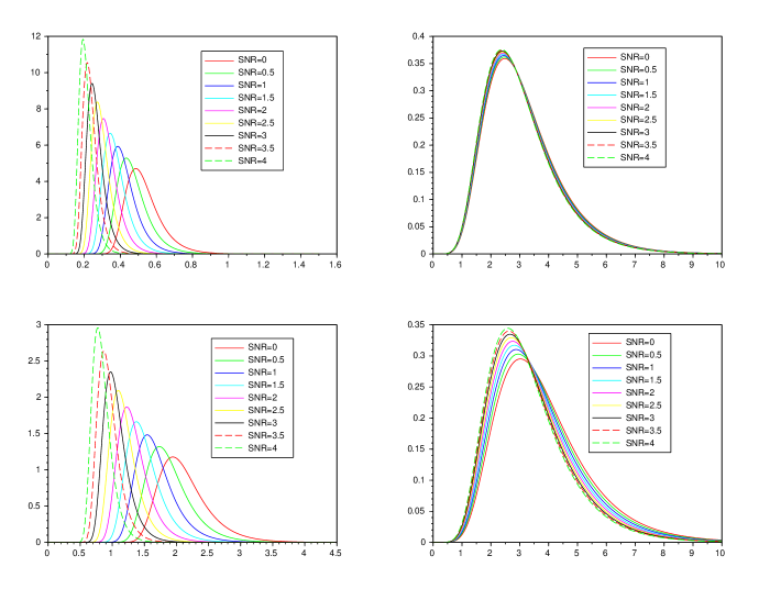
Figure 1: PDF of $Y$ and $Z$ for various SNRs, re-transmissions and $N=4$ antennas.

Figure 2: PDF of $Y$ and $Z$ for various SNRs, re-transmissions and $N=8$ antennas.

II System Model

Consider an $N\times N$ MIMO system (see Figure 1 of [9]). The channel is assumed to be quasi-static (time-invariant over one re-transmission and varies randomly over re-transmissions), frequency selective fading. The channel impulse response between transmit antenna $n_{t}$ and receive antenna $n_{r}$ for the $k^{th}$ re-transmission at time $n$ is denoted by $\tilde{h}_{k,\,n,\,n_{r},\,n_{t}}$ and is characterized by (E3) in [9]. The subscripts in the channel impulse response are integers that lie in the range $1\leq k\leq N_{rt}$, $0\leq n<L_{h}$ and $1\leq n_{r},\,n_{t}\leq N$. Note that the number of re-transmissions is denoted by $N_{rt}$, the length of the channel impulse response is $L_{h}$ and the number of antennas at the transmitter and receiver is $N$. Clearly, there are $N^{2}N_{rt}$ channel impulse responses to be estimated. This is accomplished by using the frame structure given in Figure 3(a) of [9]. Recall that in the preamble phase, only one transmit antenna is active at an time, whereas in the data phase all transmit antennas are simultaneously active. The preamble symbols are drawn from a QPSK constellation and uncoded. The received signal $\tilde{r}_{k,\,n,\,n_{r},\,n_{t},\,p}$ during the preamble phase is given by (E8) of [9]. We assume that there is no frequency offset, that is $\omega_{0}=0$ in (E8) of [9]. The effect of non-zero frequency offset is studied in the computer simulations. At the correct timing instant (perhaps a circular shift of $\tilde{r}_{k,\,n,\,n_{r},\,n_{t},\,p}$ may be necessary), the $L_{p}$-point FFT of $\tilde{r}_{k,\,n,\,n_{r},\,n_{t},\,p}$ yields (E13) in [9], which is repeated here for convenience ($0\leq i<L_{p}$, $i$ is an integer):

$$\tilde{R}_{k,\,i,\,n_{r},\,n_{t},\,p}=\tilde{H}_{k,\,i,\,n_{r},\,n_{t}}S_{1,\,i}+\tilde{W}_{k,\,i,\,n_{r},\,n_{t},\,p}.$$ (1)

The subscript “$p$” in the above equation denotes the preamble phase. Now

$$\frac{\tilde{R}_{k,\,i,\,n_{r},\,n_{t},\,p}S_{1,\,i}^{*}}{E_{s}} =\tilde{H}_{k,\,i,\,n_{r},\,n_{t}}\frac{\left|S_{1,\,i}\right|^{2}}{E_{s}}$$

$$\qquad+\frac{\tilde{W}_{k,\,i,\,n_{r},\,n_{t},\,p}S_{1,\,i}^{*}}{E_{s}}$$

$$=\tilde{H}_{k,\,i,\,n_{r},\,n_{t}}+\frac{\tilde{W}_{k,\,i,\,n_{r},\,n_{t},\,p}S_{1,\,i}^{*}}{E_{s}}$$ (2)

since (see (E10) of [9])

$$\left|S_{1,\,i}\right|^{2}=E_{s}$$ (3)

denotes the energy of the preamble. The $L_{p}$-point inverse fast Fourier transform (IFFT) of (II) yields (for $0\leq n<L_{p}$, $n$ is an integer)

$$\tilde{r}_{1,\,k,\,n,\,n_{r},\,n_{t},\,p}=\tilde{h}_{k,\,n,\,n_{r},\,n_{t}}+\tilde{w}_{1,\,k,\,n,\,n_{r},\,n_{t},\,p}$$ (4)

where the second term on the right hand side of (4) is the $L_{p}$-point IFFT of the second term on the right hand side of (II). From (4) it is clear that $0\leq n<L_{h}$ contains the channel coefficients plus noise, whereas $L_{h}\leq n<L_{p}$ contains only noise. Typically

$$L_{h}\ll L_{p}.$$ (5)

Moreover

$$\frac{1}{2}E\left[\left|\tilde{w}_{1,\,k,\,n,\,n_{r},\,n_{t},\,p}\right|^{2}\right]=\frac{\sigma^{2}_{w}}{E_{s}}$$ (6)

where $\sigma^{2}_{w}$ is the one-dimensional variance of $\tilde{w}_{k,\,n,\,n_{r},\,n_{t},\,p}$ in (E8) of [9]. For a given $k$, $n_{r}$ and $n_{t}$ let

$$\tilde{Z}_{n} =\tilde{h}_{k,\,n,\,n_{r},\,n_{t}}+\tilde{w}_{1,\,k,\,n,\,n_{r},\,n_{t},\,p}\qquad\mbox{for $0\leq n<L_{h}$}$$

$$\tilde{Y}_{n} =\tilde{w}_{1,\,k,\,n,\,n_{r},\,n_{t},\,p}\qquad\mbox{for $L_{h}\leq n<L_{p}$}.$$ (7)

Note that $\tilde{Z}_{n}$ and $\tilde{Y}_{n}$ are complex Gaussian random variables with zero-mean. Due to independence between the channel coefficients and noise

$$\frac{1}{2}E\left[\left|\tilde{Z}_{n}\right|^{2}\right] =\sigma^{2}_{f}+\frac{\sigma^{2}_{w}}{E_{s}}$$

$$\stackrel{{\scriptstyle\Delta}}{{=}}\sigma^{2}_{Z}$$

$$\frac{1}{2}E\left[\left|\tilde{Y}_{n}\right|^{2}\right] =\frac{\sigma^{2}_{w}}{E_{s}}$$

$$\stackrel{{\scriptstyle\Delta}}{{=}}\sigma^{2}_{Y}$$ (8)

where $\sigma^{2}_{f}$ is the one-dimensional variance of $\tilde{h}_{k,\,n,\,n_{r},\,n_{t}}$ (see (E3) of [9]). An erasure occurs when

$$\max_{n}\left|\tilde{Z}_{n}\right|^{2}<\max_{n}\left|\tilde{Y}_{n}\right|^{2}$$ (9)

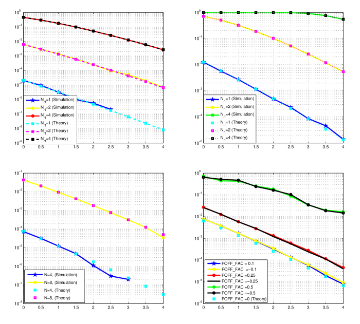
Figure 3: Simulation results.

III The Probability of Erasure

The probability density function (pdf) of $\mathscr{Z}_{n}=\left|\tilde{Z}_{n}\right|^{2}$ and $\mathscr{Y}_{n}=\left|\tilde{Y}_{n}\right|^{2}$ is given by (for $0\leq z,\,y<\infty$) [11]

$$p_{\mathscr{Z}_{n}}(z) =\frac{1}{2\sigma^{2}_{Z}}\mathrm{e}^{-z/(2\sigma^{2}_{Z})}$$

$$p_{\mathscr{Y}_{n}}(y) =\frac{1}{2\sigma^{2}_{Y}}\mathrm{e}^{-y/(2\sigma^{2}_{Y})}$$ (10)

where we have assumed that $\tilde{Z}_{n}$ and $\tilde{Y}_{n}$ are wide sense stationary, so that their pdfs are independent of the time index $n$. Let

$$\mathcal{Z} =\max_{n}\mathscr{Z}_{n}$$

$$\mathcal{Y} =\max_{n}\mathscr{Y}_{n}.$$ (11)

Since $\mathscr{Z}_{n}$ and $\mathscr{Y}_{n}$ are independent over $n$, the cumulative distribution function (cdf) of $\mathcal{Z}$ and $\mathcal{Y}$ is [12, 13]

$$P\left(\mathcal{Z}\leq z\right) =\left(P\left(\mathscr{Z}_{n}<z\right)\right)^{L_{h}}$$

$$=\left(1-\mathrm{e}^{-z/(2\sigma^{2}_{Z})}\right)^{L_{h}}$$

$$P\left(\mathcal{Y}\leq y\right) =\left(P\left(\mathscr{Y}_{n}<y\right)\right)^{L_{p}-L_{h}}$$

$$=\left(1-\mathrm{e}^{-y/(2\sigma^{2}_{Y})}\right)^{L_{p}-L_{h}}.$$ (12)

Therefore, the pdf of $\mathcal{Z}$ and $\mathcal{Y}$ are (for $0\leq z,\,y<\infty$)

$$p_{\mathcal{Z}}(z) =\frac{d}{dz}P\left(\mathcal{Z}\leq z\right)$$

$$=\frac{L_{h}}{2\sigma^{2}_{Z}}\mathrm{e}^{-z/(2\sigma^{2}_{Z})}\left(1-\mathrm{e}^{-z/(2\sigma^{2}_{Z})}\right)^{L_{h}-1}$$

$$p_{\mathcal{Y}}(y) =\frac{d}{dy}P\left(\mathcal{Y}\leq y\right)$$

$$=\frac{L_{p}-L_{h}}{2\sigma^{2}_{Y}}\mathrm{e}^{-y/(2\sigma^{2}_{Y})}\left(1-\mathrm{e}^{-y/(2\sigma^{2}_{Y})}\right)^{L_{p}-L_{h}-1}.$$

For a given $k$, $n_{r}$, $n_{t}$, and from (9) there is no erasure when

$$P_{\mathrm{ne},\,1} =\int_{z=0}^{\infty}P(\mathcal{Y}\leq z|z)p_{\mathcal{Z}}(z)\,dz$$

$$=\int_{z=0}^{\infty}\int_{y=0}^{z}p_{\mathcal{Y}}(y)\,dy\,p_{\mathcal{Z}}(z)\,dz$$ (14)

where the subscript “ne” denotes “no erasure” and “1” denotes one particular value of $k$, $n_{r}$ and $n_{t}$. Now

$$I(z) =P(\mathcal{Y}\leq z|z)$$

$$=\int_{y=0}^{z}p_{\mathcal{Y}}(y)\,dy$$

$$=\frac{L_{p}-L_{h}}{2\sigma^{2}_{Y}}\int_{y=0}^{z}\sum_{l=0}^{L_{p}-L_{h}-1}(-1)^{l}\binom{L_{p}-L_{h}-1}{l}$$

$$\qquad\times\mathrm{e}^{-(l+1)y/(2\sigma^{2}_{Y})}$$

$$=(L_{p}-L_{h})\sum_{l=0}^{L_{p}-L_{h}-1}\frac{(-1)^{l}}{l+1}\binom{L_{p}-L_{h}-1}{l}$$

$$\qquad\times\left(1-\mathrm{e}^{-(l+1)z/(2\sigma^{2}_{Y})}\right).$$ (15)

Let

$$A_{l}=\frac{L_{p}-L_{h}}{l+1}(-1)^{l}\binom{L_{p}-L_{h}-1}{l}.$$ (16)

Then

$$I(z)=\sum_{l=0}^{L_{p}-L_{h}-1}A_{l}\left(1-\mathrm{e}^{-(l+1)z/(2\sigma^{2}_{Y})}\right).$$ (17)

Therefore

$$P_{\mathrm{ne},\,1} =\int_{z=0}^{\infty}I(z)p_{\mathcal{Z}}(z)\,dz$$

$$=\int_{z=0}^{\infty}\sum_{l=0}^{L_{p}-L_{h}-1}A_{l}\left(1-\mathrm{e}^{-(l+1)z/(2\sigma^{2}_{Y})}\right)p_{\mathcal{Z}}(z)\,dz$$

$$=\frac{L_{h}}{2\sigma^{2}_{Z}}\sum_{l=0}^{L_{p}-L_{h}-1}A_{l}\left(1-\int_{z=0}^{\infty}\mathrm{e}^{-(l+1)z/(2\sigma^{2}_{Y})}\right.$$

$$\qquad\times\left.\sum_{a=0}^{L_{h}-1}(-1)^{a}\binom{L_{h}-1}{a}\mathrm{e}^{-(a+1)z/(2\sigma^{2}_{Z})}\right)\,dz$$

$$=\frac{L_{h}}{2\sigma^{2}_{Z}}\sum_{l=0}^{L_{p}-L_{h}-1}A_{l}\left(1-\sum_{a=0}^{L_{h}-1}(-1)^{a}\binom{L_{h}-1}{a}\right.$$

$$\qquad\times\left.\int_{z=0}^{\infty}\mathrm{e}^{-(l+1)z/(2\sigma^{2}_{Y})}\mathrm{e}^{-(a+1)z/(2\sigma^{2}_{Z})}\right)\,dz$$

$$=\sum_{l=0}^{L_{p}-L_{h}-1}A_{l}^{\prime}\left(1-\sum_{a=0}^{L_{h}-1}(-1)^{a}\binom{L_{h}-1}{a}\frac{1}{B_{l}+C_{a}}\right)$$

where

$$A_{l}^{\prime} =\frac{L_{h}}{2\sigma^{2}_{Z}}A_{l}$$

$$B_{l} =\frac{l+1}{2\sigma^{2}_{Y}}$$

$$C_{a} =\frac{a+1}{2\sigma^{2}_{Z}}.$$ (19)

Since the channel and noise are independent across $k$, $n_{r}$ and $n_{t}$ the probability of no erasure for all $k$, $n_{r}$ and $n_{t}$ is

$$P_{\mathrm{ne},\,\mathrm{all}}=\left(P_{\mathrm{ne},\,1}\right)^{N_{rt}N^{2}}.$$ (20)

Finally, the probability of erasure for all $k$, $n_{r}$, $n_{t}$ is

$$P_{\mathrm{e},\,\mathrm{all}}=1-P_{\mathrm{ne},\,\mathrm{all}}.$$ (21)

While it appears that (21) is the closed form expression for the probability of erasure over all re-transmissions ($k$), receive antennas ($n_{r}$) and transmit antennas ($n_{t}$), the main problem lies in the computation of $A_{l}$ in (16). The reason is that $\binom{L_{p}-L_{h}-1}{l}$ takes very large values (results in overflow) for preamble length $L_{p}=512$ and channel length $L_{h}=10$. In order to alleviate this problem, we need to resort to numerical integration techniques. Thus (III) is approximated by

$$P_{\mathrm{ne},\,1}\approx\sum_{i_{0}=0}^{N_{\mathcal{Z}}}\sum_{i_{1}=0}^{i_{0}\Delta z}p_{\mathcal{Y}}(i_{1}\Delta y)\,\Delta y\,p_{\mathcal{Z}}(i_{0}\Delta z)\,\Delta z$$ (22)

where

$$\Delta y =\Delta z$$

$$=10^{-3}$$

$$N_{\mathcal{Z}} =10^{4}$$

$$i_{0}\Delta z =z$$

$$i_{1}\Delta y =y.$$ (23)

Note that

$$N_{\mathcal{Z}}\Delta z=10.$$ (24)

In other words, it is sufficient to take the maximum value of $z$ in the upper limit of the integral over $z$ in (III) to be equal to 10. This is also clear from the plots of the pdf of $\mathcal{Z}$ in Figures 1 and 2 as a function of the average SNR per bit, the number of re-transmissions $N_{rt}$ and the number of antennas $N$. The average SNR per bit is defined in (E21) of [9], and is repeated here for convenience

$$\mbox{SNR}_{\mathrm{av},\,b,\,p}=\frac{4L_{h}\sigma^{2}_{f}NN_{rt}}{L_{d}\sigma^{2}_{w}}.$$ (25)

We find that in all cases, the pdf of $\mathcal{Z}$ goes to zero for $z>10$, which justifies the relation in (24). It can also be seen from Figures 1 and 2 that the pdf of $\mathcal{Z}$ is relatively insensitive to variations in $N$ and $N_{rt}$, whereas the pdf of $\mathcal{Y}$ varies widely with $N$ and $N_{rt}$.

IV Results

The probability of erasure results are presented in Figure 3. The results for four transmit and receive antennas ($N=4$) is shown in Figure 3(a). We see that the theoretical and simulated curves nearly coincide, which demonstrates the accuracy of our prediction. Moreover, the probability of erasure increases with increasing re-transmissions. The probability of erasure with eight transmit and receive antennas ($N=8$) is given in Figure 3(b). Clearly, the probability of erasure is three orders of magnitude higher than $N=4$, for the same number of re-transmissions $N_{rt}$. Next, in Figure 3(c), the length of the preamble and data is doubled compared to Figure 3(a) and (b), that is $L_{p}=1024$, $L_{d}=2048$ and the number of re-transmissions is fixed to $N_{rt}=2$. We see that the probability of erasure reduces by two orders of magnitude. In other words, increasing the length of the preamble ($L_{p}$) reduces the probability of erasure. Note that, when the preamble length is increased, the data length ($L_{d}$) also needs to be increased, to keep the throughput fixed (see Table 1 of [9]). Finally in Figure 3(d), we plot the probability of erasure in the presence of frequency offset ($\omega_{0}$). The received signal model in the presence of frequency offset is given by (E8) of [9], before the FFT operation at the receiver. We have taken

$$\omega_{0}=\verb!FOFF_FAC!\times\frac{2\pi}{L_{p}}$$ (26)

where $2\pi/L_{p}$ denotes the subcarrier spacing of the preamble. We see that the probability of erasure increases with increasing FOFF_FAC.

V Conclusion

In this work, we have derived the probability of erasure (defined as the probability of not detecting an OFDM frame when it is transmitted) for MIMO-OFDM systems. It is assumed that the frequency offset has been accurately estimated and cancelled. Simulation results are also presented in the presence of frequency offset, and it is seen that the probability of erasure increases with increasing frequency offset. Future work could be to derive the probability of erasure in the presence of small frequency offsets, say for $\verb!FOFF_FAC!<0.25$. The other interesting area could be to compute $\binom{a}{b}$ for large values of $a$ and $b$.

References

• [1] K.ย Vasudevan, K.ย Madhu, and S.ย Singh, โ€œData Detection in Single User Massive MIMO Using Re-Transmissions,โ€ The Open Signal Processing Journal, vol.ย 6, pp. 15โ€“26, Mar. 2019.
• [2] โ€”โ€”, โ€œScilab code for data detection in single user massive mimo using re-transmissions,โ€ https://www.codeocean.com/, 6 2019.
• [3] K.ย Vasudevan, โ€œCoherent detection of turbo-coded ofdm signals transmitted through frequency selective rayleigh fading channels with receiver diversity and increased throughput,โ€ Wireless Personal Communications, vol.ย 82, no.ย 3, pp. 1623โ€“1642, 2015. [Online]. Available: http://dx.doi.org/10.1007/s11277-015-2303-8
• [4] โ€”โ€”, Digital Communications and Signal Processing, Second edition (CDROM included).ย ย ย Universities Press (India), Hyderabad, www.universitiespress.com, 2010.
• [5] โ€”โ€”, โ€œCoherent detection of turbo coded ofdm signals transmitted through frequency selective rayleigh fading channels,โ€ in Signal Processing, Computing and Control (ISPCC), 2013 IEEE International Conference on, Sept. 2013, pp. 1โ€“6.
• [6] โ€”โ€”, โ€œScilab code for coherent detection of turbo coded ofdm signals transmitted through frequency selective rayleigh fading channels,โ€ https://www.codeocean.com/, 7 2019.
• [7] โ€”โ€”, โ€œCoherent turbo coded mimo ofdm,โ€ in ICWMC 2016, The 12th International Conference on Wireless and Mobile Communications, Nov. 2016, pp. 91โ€“99, [Online].
• [8] โ€”โ€”, โ€œNear Capacity Signaling over Fading Channels using Coherent Turbo Coded OFDM and Massive MIMO,โ€ International Journal On Advances in Telecommunications, vol.ย 10, no. 1 & 2, pp. 22โ€“37, 2017, [Online].
• [9] K.ย Vasudevan, S.ย Singh, and A.ย P.ย K. Reddy, โ€œCoherent receiver for turbo coded single-user massive mimo-ofdm with retransmissions,โ€ in Multiplexing, S.ย Mohammady, Ed.ย ย ย London: IntechOpen, 2019, ch.ย 4, pp. 1โ€“21.
• [10] โ€”โ€”, โ€œScilab code for coherent receiver for turbo coded single-user massive mimo-ofdm with retransmissions,โ€ https://www.codeocean.com/, 6 2019.
• [11] J.ย G. Proakis, Digital Communications, 3rdย ed.ย ย ย McGraw Hill, 1995.
• [12] A.ย Papoulis, Probability, Random Variables and Stochastic Processes, 3rdย ed.ย ย ย McGraw-Hill, 1991.
• [13] K.ย Vasudevan, Analog Communications: Problems & Solutions.ย ย ย Ane Books, 2018.