Robust policy search for robot navigation
with stochastic meta-policies

Abstract

Bayesian optimization is an efficient nonlinear optimization method where the queries are carefully selected to gather information about the optimum location. Thus, in the context of policy search, it has been called active policy search. The main ingredients of Bayesian optimization for sample efficiency are the probabilistic surrogate model and the optimal decision heuristics. In this work, we exploit those to provide robustness to different issues for policy search algorithms. We combine several methods and show how their interaction works better than the sum of the parts. First, to deal with input noise and provide a safe and repeatable policy we use an improved version of unscented Bayesian optimization. Then, to deal with mismodeling errors and improve exploration we use stochastic meta-policies for query selection and an adaptive kernel. We compare the proposed algorithm with previous results in several optimization benchmarks and robot tasks, such as pushing objects with a robot arm, or path finding with a rover.

I INTRODUCTION

Robot control and navigation in uncertain environments can be framed as a policy search problem [1], which has led to important achievements in robotics [2, 3, 4, 5]. Previous results had been achieved using gradient-based policy search, which might require a large number of optimization steps and a good initialization to avoid local minima. As a result, policy search typically require a large number of trials, or policy evaluations, to find a local solution.

Robot experiments are quite expensive, requiring to move and interact with a robot. Even if we use a simulator for planning or learning, robotic simulators are typically complex and computationally expensive. For example, information-based planning might be quite expensive, specially if we require also to perform localization and dense map-building simultaneously [6, 7]. Thus, sample efficiency during policy learning is of paramount importance. Active policy search uses Bayesian optimization to drive the search for optimality in an intelligent and efficient fashion. Bayesian optimization is a method for sample efficient nonlinear optimization that does not require gradients to obtain global convergence [8]. Furthermore, the probabilistic core of Bayesian optimization also allows the use of partial of incomplete information, similarly to the stochastic gradient descent commonly used in classical policy search [1]. In fact, Bayesian optimization has been already used in many robotics and reinforcement learning setups, such as robot walking [9, 10, 11], control [12, 13], planning [7, 14], grasping [15, 16] and damage recovery [17].

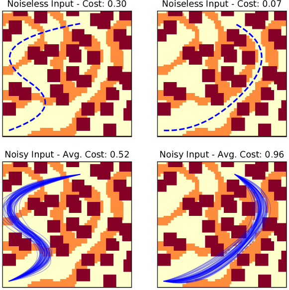
Figure 1: Path planning on uneven terrain with obstacles, with different trajectories displayed (left and right). The orange regions represents slopes with a higher traversing cost. The red rectangles are obstacles. Top: the desired trajectories (blue dashed line). Bottom: possible deviations (blue lines) from desired trajectories due to input noise. The right trajectory is more efficient without input noise. Once we take into account input noise, it becomes unsafe as it can collide with obstacles easily. The left trajectory is safer in the presence of input noise despite being less efficient.

Bayesian optimization relies on a probabilistic surrogate model of the target function, typically a Gaussian process. In the original formulation, this model is incorporated for sample efficiency [18]. In addition, the surrogate model can also be used for secondary tasks that can be useful in robotics scenarios, such as, guaranteeing a minimum outcome [19], detect and remove outliers [20] or incorporate prior information [17]. However, the surrogate model must be simple enough that it can be learned using few samples, as intended within the Bayesian optimization context. This simplicity results in certain assumptions about the surrogate model, such as spatial stationarity, that might not be satisfied when applied to policy search [21]. In this work, we propose several methods to incorporate robustness to mismodeling errors and assumptions. First, we use an adaptive surrogate model for nonstationary environments [21]. Bayesian optimization also relies on optimal decision theory to actively select the most informative trial to find the optimal result. When combined with a biased model, this can lead to poor results and lack of convergence. Thus, we have also incorporated a decision rule based on stochastic meta-policies that can be robust to surrogate modeling errors [22]. The intuition behind the meta-policies is to consider the Bayesian optimization component as a meta reinforcement learning problem on top of the actual policy search problem. Another advantage of the stochastic meta-policies is that they trivially allow to perform distributed Bayesian optimization in a multi-robot setup or using a simulator in a computer cluster.

In the case of robotic applications, localization or trajectory uncertainty should also be considered. The optimal policy should be able to be effectively followed by the robot if we need to repeat the task multiple times. For example, take the path planning problem from Figure 1, although the right trajectory is more cost efficient, as we introduce input noise, it becomes unsafe and incurs on a higher cost on average. On the contrary, the left trajectory is less cost efficient without input noise, but at a certain input noise it becomes a safe and efficient route. If we think on the cost function in terms of the policy parameters, we can see that the left trajectory lies in a smooth flat region while the right trajectory lies in a high variance region with a narrow valley. Thus, depending on the task or environmental conditions, the algorithm should able to select between narrow and flat optimum regions. In this work, we combine previous works on Bayesian optimization input noise [15] and adaptive kernels [23], which allows to get the best solution for each situation. Furthermore, we provide a new interpretation of unscented Bayesian optimization [15] as an integrated response method and a new formulation based on the scaled unscented transform.

II ACTIVE POLICY SEARCH

Policy search consists of finding the optimal parameters $\mathbf{x}^{*}$ of a policy $\pi_{\mathbf{x}}(\mathbf{a}_{k}|\mathbf{s}_{k})$, which is a distribution over actions $\mathbf{a}_{k}$ conditioned on states $\mathbf{s}_{k}$, with respect to the expectation future return $U^{\pi}$, denoted $\mathbb{E}[U^{\pi}]=\mathbb{E}[\sum_{k=1}^{M}R^{\pi}(\mathbf{s}_{k},\mathbf{a}_{k})]$. The expectation is under the policy and the system dynamics which together form a distribution over trajectories $\tau$. If we use an episodic formulation, such as REINFORCE [1], the expectation is usually approximated from Monte-Carlo rollouts $\tau^{(i)}\sim\tau$ of the robot trajectory. In this setup, finding the optimal policy parameters can be framed as a pure optimization problem, where the objective function is then computed as:

$$\begin{split}f(\mathbf{x})&=\mathbb{E}_{\tau}[U^{\pi}]\approx\sum_{i=1}^{N}\sum_{k=1}^{M}R\left(\tau_{k}^{(i)}\right)\\ \mathbf{x}^{*}&=\arg\max_{\mathbf{x}\in\mathcal{X}}\mathbb{E}_{\tau}[U^{\pi}]\end{split}$$ (1)

where $\mathbf{x}^{*}$ are the parameters of the optimal policy $\pi^{*}=\pi_{\mathbf{x}^{*}}$, $R(\tau_{k}^{(i)})$ is the instantaneous reward at time step $k$ following rollout $\tau^{(i)}$. Active policy search [6] computes the optimal policy parameters using Bayesian optimization. Similarly to stochastic gradient descent in gradient-based policy search, Bayesian optimization can directly be applied to stochastic optimization thanks to the probabilistic surrogate model [24]. Therefore, the expectation in equation (1) can be approximated with a small batch of rollouts or even a single episode. Algorithm 1 summarized the active policy search strategy. Section III details the steps of updating the surrogate model and generating the next set of policy parameters $\mathbf{x}_{t+1}$

Algorithm 1 Active Policy Search

1:Optimization budget $T$

2:Initialize $\mathbf{x}_{1}$ based on a low discrepancy sequence.

3:for each optimization iteration $t$ until budget $T$ do:

4:     Generate episode $\tau_{\mathbf{x}_{t}}\sim\{s_{0},a_{0},R_{1},s_{1},a_{1},\ldots\}$

5:     $y_{t}\leftarrow\sum_{k=1}^{M}R_{k}$

6:     Add $(\mathbf{x}_{t},y_{t})$ to surrogate model with equation (3)

7:     Generate $\mathbf{x}_{t+1}$ using equation (2)

8:end for

III BAYESIAN OPTIMIZATION

Bayesian optimization (BO) is a framework that aims to efficiently optimize noisy, expensive, blackbox functions. It uses two distinct components: a probabilistic surrogate model $p(f)$ that learns the properties and features of the target function using previously evaluated observations and an acquisition function $\alpha(x,p(f))$ that, based on the surrogate model, builds an utility function which rates how promising a subsequent query could be. For the remainder of the paper, the discussion and results are based on the use of a Gaussian process (GP) as the surrogate model and the expected improvement (EI) as the acquisition function because they are the most commonly used in the literature due to their excellent performance in a large variety of problems.

Formally, BO attempts to find the global optima of an expensive unknown function $f:\mathcal{X}\to\mathbb{R}$ over some domain $\mathcal{X}\subset\mathbb{R}^{d}$ by sequentially performing queries. At iteration $t$, all previously observed values $\mathbf{y}=y_{1:t}$ at queried points $\mathbf{X}=\mathbf{x}_{1:t}$ are used to learn a probabilistic surrogate model $p(f|y_{1:t},\mathbf{x}_{1:t})$. Typically, the next query $\mathbf{x}_{t+1}$ is then determined by greedily optimizing the acquisition function in $\mathcal{X}$:

$$\mathbf{x}_{t+1}=\arg\max_{\mathbf{x}\in\mathcal{X}}\alpha\left(\mathbf{x},p(f\;|\;y_{1:t},\mathbf{x}_{1:t})\right)$$ (2)

although we will replace the greedy selection in Section V-B.

Surrogate Model

As commented previously, the most common surrogate model is the Gaussian process (GP). For the remainder of the paper we consider a GP with zero mean and kernel $k:\mathcal{X}\times\mathcal{X}\to\mathbb{R}$ with hyperparameters $\boldsymbol{\theta}$. The GP posterior model allows predictions at a query point $\mathbf{x}_{q}$ which are normally distributed $y_{q}\sim\mathcal{N}(\mu(\mathbf{x}_{q}),\sigma^{2}(\mathbf{x}_{q}))$, such that:

$$\begin{split}\mu(\mathbf{x}_{q})&=\mathbf{k}(\mathbf{x}_{q})^{T}\mathbf{K}^{-1}\mathbf{y}\\ \sigma^{2}(\mathbf{x}_{q})&=k(\mathbf{x}_{q},\mathbf{x}_{q})-\mathbf{k}(\mathbf{x}_{q})^{T}\mathbf{K}^{-1}\mathbf{k}(\mathbf{x}_{q})\end{split}$$ (3)

where $\mathbf{k}(\mathbf{x}_{q})=\left[k(\mathbf{x}_{q},\mathbf{x}_{i})\right]_{\mathbf{x}_{i}\in\mathbf{X}}$ and $\mathbf{K}=\left[\mathbf{k}(\mathbf{x}_{i},\mathbf{x}_{j})\right]_{\mathbf{x}_{i},\mathbf{x}_{j}\in\mathbf{X}}+\mathbf{I}\sigma^{2}_{n}$. For the kernel, we have used the Spartan kernel [23] which provides robustness to nonstationary function and improves convergence. The use of the kernel is further explained in Section V-A.

Acquisition Function

The expected improvement (EI) [25] is an standard acquisition function defined in terms of the query improvement at iteration $t$ and is defined as:

$$EI_{t}(\mathbf{x})=\left(\rho_{t}-\mu_{t}\right)\Phi(z_{t})+\sigma_{t}\phi(z_{t})$$ (4)

where $\phi$ and $\Phi$ are the corresponding Gaussian probability density function (PDF) and cumulative density function (CDF), being $z_{t}=(\rho_{t}-\mu_{t})/\sigma_{t}$. In this case, $(\mu,\sigma^{2})$ are the prediction parameters computed with (3) and $\rho_{t}=\max(y_{1},\ldots,y_{t})$ is the incumbent optimum at that iteration.

Hyperparameters

The GP formulation provides a nice closed-form computation of predictive distributions. However, the kernel hyperparameters $\boldsymbol{\theta}$ introduce nonlinearity and non-Gaussianity that breaks the closed-form solution. In many applications of GPs, including Bayesian optimization, the empirical Bayes approach is employed where a point estimate is used, resulting in an overconfident estimate of the GP uncertainty [26]. Instead, we use a fully Bayesian approach based on Markov chain Monte Carlo (MCMC) to generate a set of samples $\{\boldsymbol{\theta}_{i}\}_{i=1}^{N}$ with $\boldsymbol{\theta}_{i}\sim p(\boldsymbol{\theta}|\mathbf{y},\mathbf{X})$. In particular, we use the slice sampling algorithm which has already been used successfully in Bayesian optimization [27]. In this case, the resulting acquisition function has to be approximated by the Monte Carlo counterpart:

$$EI_{t}(\mathbf{x})=\sum_{i=1}^{N}EI_{t}^{(i)}(\mathbf{x})$$ (5)

Initialization

During the first iterations, EI is known to be unstable due to lack of information [18, 28]. Therefore, the optimization is initialized with $p$ evaluations from a low discrepancy sequence, like the Sobol sequence, before we start using the acquisition function to decide the location of the next query.

IV ROBUSTNESS TO INPUT NOISE

Local robustness in optimization can be achieved by performing sensitivity analysis of the optimum selection. In Bayesian optimization, this can be performed online thanks to the surrogate model. Instead of selecting the point that optimizes a single outcome, we select the point that optimizes an integrated outcome:

$$g(\mathbf{x})=\int_{\mathcal{X}}f(\mathbf{x})p(\mathbf{x})d\mathbf{x}$$ (6)

where $p(\mathbf{x})$ can be interpreted objectively as input noise or, subjectively, as a probabilistic representation of the local stability or safety region. That is, a region that guarantees good results even if the query is repeated several times. Instead of $f(\cdot)$, the integrated outcome $g(\cdot)$ becomes the function that will be optimized. This has been previously studied in the context of Bayesian optimization using the unscented transformation [15, 29]. Input noise has also been addressed [30, 31], however the former focuses on worst case scenarios of the input noise [30], while the latter is designed to find unstable global optima despite input noise [31]. In this paper, we use a more flexible variant of the unscented transformation, called the scaled unscented transformation [32], to allow more control on the stability region and avoid numerical issues. Note that, contrary to previous works that focus on finding stable/safe regions, we consider the more challenging scenario of input noise, where the objective is not only to find a broad maximum, but queries are also perturbed $\mathbf{x}\pm\Delta\mathbf{x}$.

IV-A Scaled unscented Bayesian optimization

The unscented transformation (UT) is a method to propagate probability distributions through nonlinear transformations with a trade off of computational cost vs accuracy. It is based on the principle that it is easier to approximate a probability distribution than to approximate an arbitrary nonlinear function [33]. The unscented transformation uses a set of deterministically selected samples from the original distribution (called sigma points) and transform them through the nonlinear function $f(\cdot)$. Then, the transformed distribution is computed based on the weighted combination of the transformed sigma points:

$$\left\{\bar{\mathbf{x}},\;\bar{\mathbf{x}}\pm\left(\sqrt{(d+\gamma)\Sigma_{\mathbf{x}}}\right)_{i}\right\}\qquad\forall\;i=1\ldots d$$ (7)

where $(\sqrt{\cdot})_{i}$ is the i-th row or column of the corresponding matrix square root and $\gamma=\alpha^{2}(d+\kappa)-d$. The weight for the initial point is $w^{0}=\frac{\gamma}{d+\gamma}$ and $w^{(i)}=\frac{1}{2(d+\gamma)}$ for the rest. The parameters should follow $\kappa\geq 0$ and $0\leq\alpha\leq 1$. As pointed out by van der Merwe [34], we recommend a $\kappa=0$ and $\alpha$ close to $1$. For the matrix square root function, we use the Cholesky decomposition for its numerical stability and robustness [34].

The unscented transformation is used twice in our algorithm. First, it is used to drive the search towards stable optimum by computing the unscented expected improvement. However, there might be some cases where unstable optima are found by chance. Therefore, we further compute the unscented optimal incumbent which selects the most stable optimum among those predicted by the surrogate model. We define the unscented optimal incumbent $\widetilde{\rho}_{t}$ and its corresponding input vector $\widetilde{\mathbf{x}}_{t}$ as:

$$\widetilde{\mathbf{x}}_{t}=\arg\max_{\mathbf{x}\in\mathbf{X}}g(\mathbf{x})\qquad\text{with}\qquad\widetilde{\rho}_{t}=g(\widetilde{\mathbf{x}}_{t})$$ (8)

In this case, the output of the optimization process is the final optimal incumbent $\{\widetilde{\mathbf{x}_{T}},\widetilde{\rho_{T}}\}$

IV-B The Unscented transform as integration

Although the unscented transformation was designed for propagation of probability distribution through nonlinear functions, it can be also interpreted as a probabilistic integration. In fact, the unscented transformation with $\alpha=1$ and $\kappa=0$ is equivalent to the three point Gauss-Hermite quadrature rule [34]. While the Gauss-Hermite method computes the integral exactly under the Gaussian assumption, it has a cost of $\mathcal{O}(n^{d})$ where $n$ is the polynomial order of the function in the region. Meanwhile the unscented transform, has a quadratic cost $\mathcal{O}(d^{2})$ for computing the expected value [34]. The low cost of the unscented transformation is also an advantage compared to other more advanced integration methods such as Monte Carlo or Bayesian quadrature, which have higher computational cost.

Note that, during optimization the integrated outcome $g(\mathbf{x})$ is always applied with respect to the surrogate model $\widehat{f}(\mathbf{x})$ to avoid increasing the number of queries to $f(\mathbf{x})$. Therefore, the integral would be as accurate as the Gaussian process with respect to the target function. We found that, in practice, it is more efficient to employ the computational resources to improve the surrogate model, than to provide a better integrated outcome. Furthermore, the unscented transform also computes the full posterior uncertainty, which can be used for further Bayesian analysis and hierarchical decision models that the integrated outcome of (6).

V ROBUSTNESS TO MISMODELING ERRORS

In this section, we also consider different sources of modeling errors and methods to deal with them.

V-A Adaptive nonstationarity

Consider again the example from Figure 1. Given that the optimum can be either trajectory depending on the input noise level, our optimization algorithm must be able to model both if needed. Thus, it might also require to find very narrow optima in nonstationary spaces, which is known to be problematic for GP-based BO. Furthermore, it has been previously shown that reward functions in robotics environments are typically nonstationary [21]. This presents a problem for standard Bayesian optimization which assumes spatial stationarity of the target function. For that reason, we have incorporated the Spartan kernel [23] which combines a local and a global kernel to allow better modelling of complex functions.

This composite kernel is the combination of a kernel with global influence with several kernels with moving local influence. The influence is determined by a weighting function. The influence of the local kernels is centered in a single point with multiple diameters, creating a funnel structure:

$$\begin{split}k_{S}(\mathbf{x},\mathbf{x}^{\prime}|\boldsymbol{\theta}_{S})&=\lambda_{g}(\mathbf{x})\lambda_{g}(\mathbf{x}^{\prime})k_{g}(\mathbf{x},\mathbf{x}^{\prime}|\boldsymbol{\theta}_{g})\\ &+\sum_{l=1}^{M}\lambda_{l}(\mathbf{x}|\boldsymbol{\theta}_{p})\lambda_{l}(\mathbf{x}^{\prime}|\boldsymbol{\theta}_{p})k_{l}(\mathbf{x},\mathbf{x}^{\prime}|\boldsymbol{\theta}_{l})\end{split}$$ (9)

where the weighting function for the local kernel $\lambda_{l}(\mathbf{x}|\boldsymbol{\theta}_{p})$ includes the parameters to move the center of the local kernels along the input space. In order to achieve smooth interpolation between regions, each region have an associated weighting function $\omega_{j}(\mathbf{x})$, having the maximum in the corresponding region $j$ and decreasing its value with distance to region $j$ [23]. Then, we can set $\lambda_{j}(\mathbf{x})=\sqrt{\omega_{j}(\mathbf{x})/\sum_{p}\omega_{p}(\mathbf{x})}$. The unnormalized weights $\omega$ are defined as:

$$\begin{split}\omega_{g}&=\mathcal{N}\left(\psi,\mathbf{I}\sigma^{2}_{g}\right),\\ \omega_{l}&=\mathcal{N}\left(\boldsymbol{\theta}_{p},\mathbf{I}\sigma^{2}_{l}\right)\qquad\forall\;l=1\ldots M\end{split}$$ (10)

where $\psi$ and $\boldsymbol{\theta}_{p}$ can be seen as the center of the influence region of each kernel while $\sigma_{g}$ and $\sigma_{l}$ are related to the diameter of the area of influence. Note that all the local kernels share the same position (mean value) but different size (variance), generating a funnel-like structure.

For the local kernels, we estimate the center of the funnel structure $\boldsymbol{\theta}_{p}$ based on the data gathered. We propose to consider $\boldsymbol{\theta}_{p}$ as part of the hyperparameters for the Spartan kernel, which also includes the parameters of the local and global kernels, that is,

$$\boldsymbol{\theta}_{S}=[\boldsymbol{\theta}_{g},\boldsymbol{\theta}_{l_{1}},\ldots,\boldsymbol{\theta}_{l_{M}},\boldsymbol{\theta}_{p}]$$ (11)

In the experiments, we have used a single local Matérn kernel with automatic relevance determination of the hyperparameters [26, 23]. The global kernel is also a Matérn kernel with the same prior on the hyperparameters.

V-B Stochastic meta-policies

TABLE I: Comparison of POMDP and BO terms

POMDPs	Bayesian optimization
State: $s_{t}$	Target function: $f$
Action: $a_{t}$	Next query: $x_{t+1}$
Observation: $y_{t}$	Response value: $y_{t}=f(x_{t})$
Belief: $b_{t}=p(s_{t})$	Surrogate model: $p(f)$
Q-function: $Q^{*}(b_{t},a_{t})$	Acquisition function: $\alpha(x,p(f))$
Reward: $R(s_{t},a_{t})$	Improvement: $\max(0,y_{t+1}-\rho_{t})$

As a sequential decision making process, we can interpret the Bayesian optimization framework as a partially observable Markov decision process (POMDP) [35, 22]. In this interpretation, the state is the target function, the action is the next query point, the belief is the surrogate model and the action-value (Q-function) is the acquisition function for each possible query. Table I contains a comparison between the elements of both frameworks. Note that this POMDP model would represent the learning process of the actual policy search. Then, equation (2) can be seen as a meta-policy, because it is used to learn the actual policy $\pi_{\mathbf{x}}$. We can see that the Bayesian optimization meta-policies that can be found in the literature are spatially greedy, that is, they select the action or next query that maximizes the acquisition function or Q-function.

In the reinforcement learning literature, the stochastic policy can be used to improve exploration and increase the performance when the model is not accurate, as mismodelling errors might result in a lack of convergence of greedy policies. Mismodelling errors are also common in Bayesian optimization by selecting a specific surrogate model (GP, random forest, Bayesian NN…) we introduce some assumptions that the target function might not satisfy, as discussed in Section V-A. Furthermore, having input noise during the optimization is another source of misleading observations, as the observed query will deviate from the intended query.

Our approach consist on replacing the greedy policy of equation (2) with a stochastic policy such as the following Boltzmann policy (also known as Gibbs or softmax policy):

$$p(\mathbf{x}_{t+1}\;|\;y_{1:t},\mathbf{x}_{1:t})=\frac{e^{\beta_{t}\alpha\left(x_{t+1},p(f\;|\;y_{1:t},\mathbf{x}_{1:t})\right)}}{\int_{x\in\mathcal{X}}e^{\beta_{t}\alpha\left(x,p(f\;|\;y_{1:t},\mathbf{x}_{1:t})\right)}dx}$$ (12)

wich defines a probability distribution for the next query or action [22]. Thus, the actual next query is selected by sampling that distribution $\mathbf{x}_{t+1}\sim p(\mathbf{x}_{t+1}\;|\;y_{1:t},\mathbf{x}_{1:t})$. This policy allows exploration even if the model is completely biased. This approach can be applied to any acquisition function or surrogate model that can be found in the literature.

V-C Distributed Bayesian optimization

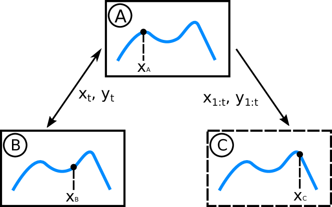
Figure 2: Illustration of a fully distributed BO architecture where each of the nodes perform BO. In the example, nodes A and B are already up and working with different random seeds. We want to spin up a new node C during optimization. A and B run independently and only need to broadcast their new queries and observations. C needs all previous queries and observations up to the current instant $t$ to start working in the same way as A and B. No state or model needs to be transferred.

A secondary advantage of the stochastic meta-policies is that they also trivially enable distributed optimization, where different policy parameters can be evaluated in parallel in a fully distributed fashion. This could be applied in multi-robot scenarios or for simulation-based reinforcement learning. Most parallel and batch BO methods require a central node to keep track of the computed and deployed queries in order to ensure that parallel queries are diverse. Without this central node, different nodes can evaluate the same query independently due to the maximum in equation (2). Many parallel methods for Bayesian optimization have been proposed in the past few years with heuristics to enforce diverse queries. Some authors include artificially augmented data by hallucinated observations [36, 27] or combine optimization with some degree of active learning in order maximize the knowledge about the target function [37, 38, 39] or enforcing spatial coverage [40].

Sampling from the stochastic policy already ensures diverse queries [22]. It does not require a centralized node and all the computation can be done in each node in a fully distributed manner in multiple nodes as shown in Figure 2. Furthermore, for optimal results, the nodes only need to broadcast their latest evaluated query and observation value $\{\mathbf{x}_{t},y_{t}\}$, requiring minimal communication bandwidth. In addition to that, communication can be asynchronous and be even robust to failures in the network, as the order of the queries and observations is irrelevant.

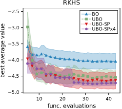
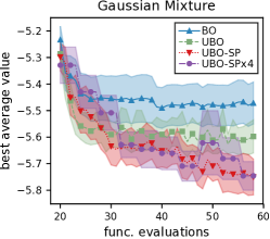
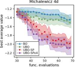
Figure 3: Benchmark functions optimization results. In general, UBO is able to find a more stable solution than the vanilla BO, resulting in a better average value. However, using stochastic meta-policies results in an improved stability. Parallelized runs had a much lower walltime without a penalty in performance.

VI RESULTS

In this section we describe the experiments used to compare the performance of different Bayesian optimization methods in the presence of input noise. We compare a vanilla implementation of Bayesian optimization (BO), the unscented Bayesian optimization (UBO) with a greedy policy and UBO with the stochastic meta-policy (UBO-SP). We also include in the comparison a parallelized version of stochastic policy applied to UBO with 4 nodes (UBO-SPx4) to study the performance impact of adding parallelization. Note that in the results we show the number of function evaluations, not iterations. For example, at the 20 evaluation, the UBO-SPx4 method had run only for 5 iterations, therefore requiring less wall time and using only the information of 16 points, instead of 19.

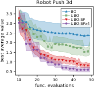
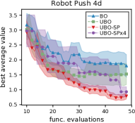
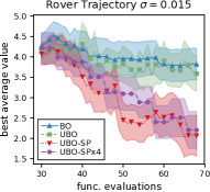
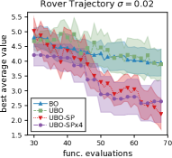
Figure 4: Robot pushing problem and rover path planning optimization results. For the more complex problems, the UBO is not able to find a stable solution, but the stochastic meta-policy does. Only for the 4D robot push, there is a penalty of using the parallel version.

As discussed previously, all methods share the same configuration: expected improvement (EI) as the acquisition function and a Gaussian process as the surrogate model with the Spartan kernel and MCMC for the hyperparameters. The initial samples are taken from a Sobol sequence. We normalize the input of all the problems between 0 and 1, so the reported input noise already assumes that the input is normalized.

The performance of each method was evaluated in the following way: For every function evaluation $\mathbf{x}_{t}$, each method computes their best solution (the optimal incumbent $\rho_{t}$ or the unscented optimal incumbent $\widetilde{\rho}_{t}$) using the observations $(\mathbf{x}_{1:t},y_{1:t})$ and according to their model at that point of the optimization. Then, we evaluate the integrated outcome at the best solution $g(\widetilde{\mathbf{x}}_{t})$ by approximating (6) using 1000 Monte Carlo samples from $p(\mathbf{x})$ over the actual function $f(\cdot)$. For the plots, we repeat each optimization 20 times and display the mean value with 95% confidence interval. Common random numbers where used for all the methods.

VI-A Benchmark Optimization Functions

First, we have evaluated the methods on synthetic benchmark functions for optimization. We have used the functions from Nogueira et al. [15], the RKHS function [41] and a Mixture of 2D Gaussian distributions (GM). These functions have unstable global optima for certain levels of input noise. This means that in order to locate the safe optima, we need to model and take into account the input noise. We have also used a 4D Michalewicz function, a popular test problem for global optimization because its sharp edges and the large number of local optima. All benchmark functions use input noise $\sigma=0.02$ and 40 evaluations. Number of initial samples is set based on the dimensionality of each problem to 5, 20 and 30 samples for RKHS, GM and Michalewicz respectively.

Figure 3 shows the results on the benchmark functions. We can see how UBO is able to find better stable optima than vanilla BO and how introducing an stochastic meta-policy to the unscented method (UBO-SP) further improves the performance. It also shows that if we choose to add parallelization, it barely impacts the optimization results. This means that we can achieve better performance and better wall-time using parallel stochastic meta-policy.

BO:
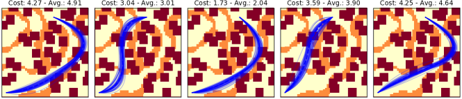
UBO:
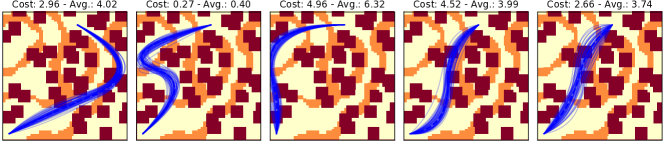
UBO-SP:
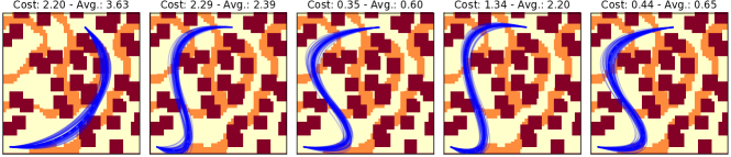
UBO-SPx4:

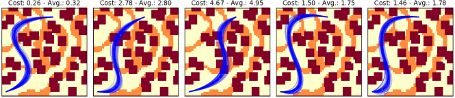
Figure 5: Examples of optimized trajectories found by different methods (rows) and trials (columns), showing the possible deviations from the trajectories by simulating input noise $\sigma=0.02$. We display the cost of the desired trajectory (assuming no input noise) and the average cost from possible deviations over each result.

BO:
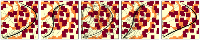
UBO:
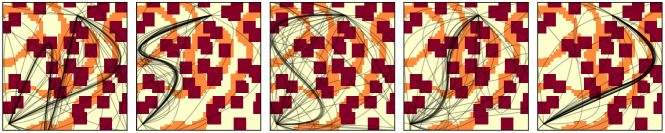
UBO-SP:
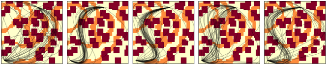
UBO-SPx4:

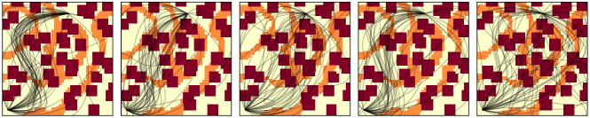
Figure 6: Overlapping rover trajectories evaluated during optimization, for different methods (rows) and trials (columns) with input noise $\sigma=0.02$. This allow us to visualize the effect of greedy and stochastic meta-policies in the optimization. We can see how greedy methods (Default-EI and UBO-EI) are more prone to over-sample similar trajectories while stochastic methods (UBO-SP-EI and UBO-SPx4-EI) performs more exploration of trajectories.

VI-B Robot Pushing

Next, we have used the active learning for robot pushing setup and code from Wang et al. [42]. The task is to perform active policy search for pushing an object towards a designated goal location. In the 3D version, the policy parameters are the robot location $(r_{x},r_{y})$ and pushing duration $t_{r}$. An alternative 4D function is also used, adding the robot angle $r_{\theta}$ as a fourth parameter. These functions have also been used previously to study robust Bayesian optimization [30]. In both functions, we use 10 initial queries and a budget of 40 function evaluations during optimization. The 3D version uses $\sigma=0.02$ while the 4D version uses $\sigma=0.01$. We reduced the input noise in the 4D function because the robot angle parameter $r_{\theta}$ is very sensitive to input noise, as a small change in direction of the robot might result in completely missing the goal.

Figure 4, shows the results of Robot Pushing problem. In both functions the results are consistent with the experiments on benchmark functions. In general, applying UBO improves the performance over BO and, by introducing an stochastic meta-policies, UBO-SP and UBO-SPx4 further enhances exploration and improves robustness and, thus, the overall performance.

VI-C Robot Path Planning

In this section we cover the problem of safe path planning. The objective is to find a stable and efficient trajectory of a rover through a rugged terrain with multiple obstacles. It is based on optimizing rover trajectories from Wang et al. [43]. In this case, there are 4 policy parameters. We designed a new environment in which a rover has to perform path planning while avoiding obstacles, which might be dangerous for the rover to collide with, and changes in elevation, which might be dangerous as the rover can tip over. In the figures, obstacles are red rectangles and slopes are orange regions. Uncertainty following the desired trajectory is represented as input noise in the trajectory parameters, meaning that we are interested in finding stable trajectories that avoid the danger that might arise from possible deviations. This is a common problem in robot navigation as localization errors might results in the robot not following the desired trajectory accurately [6, 7].

We study this problem using 2 different input noise: $\sigma=0.015$ and $\sigma=0.02$. In both cases, we use 30 initial samples and 40 function evaluations during optimization. Figure 4 shows the resulting optimization performance of each of the methods. Figure 5 shows some trajectories obtained using different methods. In this problem, applying UBO is not enough, as the results show that it does not improve over BO. In order to understand why, we study the function evaluations performed by each method, shown in Figure 6. We can see how, greedy methods cannot recover from a biased models as shown by the high density of the trajectories. Contrary to that, the stochastic approach do not suffer from it and keep exploring with different trajectories. This shows how UBO-SP and UBO-SPx4 methods are more robust to mismodeling errors and how the improved exploration helps in finding better safe trajectories.

VII CONCLUSIONS

In this paper, we propose the first active policy search algorithm that offers robustness to input noise and mismodeling errors using unscented Bayesian optimization with stochastic meta-policies. First, we have presented a new formulation and interpretation of the UBO algorithm. Second, we have combined the UBO algorithm with the Spartan kernel to deal with nonstationary functions and an stochastic meta-policy for mismodeling robustness and evaluated it on several benchmark functions and robotic applications that showcase the influence of input noise, such as safe robot navigation; confirming that, the synergies of both methods (UBO and stochastic meta-policy) results in improved robustness over the methods separately. This further highlights previous results that indicates that the ubiquitous greedy strategy in the Bayesian optimization literature can be suboptimal in many applications. We also take advantage of the embarrassingly parallel nature of the stochastic meta-policies that could be using in multi-robot setups or simulation enviroments.

References

- [1] R. J. Williams, “Simple statistical gradient-following algorithms for connectionist reinforcement learning,” Machine learning, vol. 8, no. 3-4, pp. 229–256, 1992.
- [2] M. Deisenroth, G. Neumann, and J. Peters, “A survey on policy search for robotics,” Foundations and Trends in Robotics, vol. 2, no. 1-2, pp. 1–142, 2013.
- [3] J. Peters and S. Schaal, “Policy gradient methods for robotics,” in Proc. of the IEEE/RSJ Int. Conf. on Intelligent Robots and Systems, 2006.
- [4] N. Kohl and P. Stone, “Policy gradient reinforcement learning for fast quadrupedal locomotion,” in Proc. of the IEEE Int. Conf. on Robotics & Automation, 2004.
- [5] S. Levine and P. Abbeel, “Learning neural network policies with guided policy search under unknown dynamics,” in Advances in Neural Information Processing Systems, 2014, pp. 1071–1079.
- [6] R. Martinez-Cantin, N. de Freitas, A. Doucet, and J. A. Castellanos, “Active policy learning for robot planning and exploration under uncertainty,” in Robotics: Science and Systems, 2007.
- [7] R. Martinez-Cantin, N. de Freitas, E. Brochu, J. Castellanos, and A. Doucet, “A Bayesian exploration-exploitation approach for optimal online sensing and planning with a visually guided mobile robot.” Autonomous Robots, vol. 27, no. 3, pp. 93–103, 2009.
- [8] B. Shahriari, K. Swersky, Z. Wang, R. Adams, and N. de Freitas, “Taking the human out of the loop: A review of Bayesian optimization,” Proceedings of the IEEE, vol. 104, no. 1, pp. 148–175, 2016.
- [9] D. Lizotte, T. Wang, M. Bowling, and D. Schuurmans., “Automatic gait optimization with gaussian process regression,” in IJCAI, 2007, pp. 944–949.
- [10] R. Calandra, A. Seyfarth, J. Peters, and M. Deisenroth, “Bayesian optimization for learning gaits under uncertainty,” Annals of Mathematics and Artificial Intelligence (AMAI), vol. 1 1, pp. 1–19 1–19, 2015.
- [11] A. Rai, R. Antonova, F. Meier, and C. G. Atkeson, “Using simulation to improve sample-efficiency of bayesian optimization for bipedal robots.” Journal of machine learning research, vol. 20, no. 49, pp. 1–24, 2019.
- [12] M. Tesch, J. Schneider, and H. Choset, “Adapting control policies for expensive systems to changing environments,” in IEEE/RSJ International Conference on Intelligent Robots and Systems, 2011.
- [13] S. R. Kuindersma, R. A. Grupen, and A. G. Barto, “Variable risk control via stochastic optimization,” The International Journal of Robotics Research, vol. 32, no. 7, pp. 806–825, 2013.
- [14] R. Marchant and F. Ramos, “Bayesian optimisation for informative continuous path planning,” in Robotics and Automation (ICRA), 2014 IEEE International Conference on. IEEE, 2014, pp. 6136–6143.
- [15] J. Nogueira, R. Martinez-Cantin, A. Bernardino, and L. Jamone, “Unscented bayesian optimization for safe robot grasping,” in 2016 IEEE/RSJ International Conference on Intelligent Robots and Systems (IROS). IEEE, 2016, pp. 1967–1972.
- [16] C. Daniel, O. Kroemer, M. Viering, J. Metz, and J. Peters, “Active reward learning with a novel acquisition function,” Autonomous Robots, vol. 39, no. 3, pp. 389–405, 2015.
- [17] A. Cully, J. Clune, D. Tarapore, and J. B. Mouret, “Robots that can adapt like animals,” Nature, vol. 521, p. 503–507, 2015.
- [18] D. R. Jones, M. Schonlau, and W. J. Welch, “Efficient global optimization of expensive black-box functions,” Journal of Global Optimization, vol. 13, no. 4, pp. 455–492, 1998.
- [19] Y. Sui, A. Gotovos, J. Burdick, and A. Krause, “Safe exploration for optimization with gaussian processes,” in International Conference on Machine Learning, 2015, pp. 997–1005.
- [20] R. Martinez-Cantin, K. Tee, and M. McCourt, “Practical bayesian optimization in the presence of outliers,” in International Conference on Artificial Intelligence and Statistics, 2018, pp. 1722–1731.
- [21] R. Martinez-Cantin, “Bayesian optimization with adaptive kernels for robot control,” in Proc. of the IEEE International Conference on Robotics and Automation, 2017, pp. 3350–3356.
- [22] J. Garcia-Barcos and R. Martinez-Cantin, “Fully distributed bayesian optimization with stochastic policies,” in Proceedings of the Twenty-Eighth International Joint Conference on Artificial Intelligence, IJCAI-19, 2019, pp. 2357–2363.
- [23] R. Martinez-Cantin, “Funneled Bayesian optimization for design, tuning and control of autonomous systems,” IEEE Trans Cybern, vol. 49, no. 4, pp. 1489–1500, 2019.
- [24] D. Huang, T. T. Allen, W. I. Notz, and N. Zheng, “Global optimization of stochastic black-box systems via sequential kriging meta-models,” Journal of Global Optimization, vol. 34, no. 3, pp. 441– 466, 2006.
- [25] J. Mockus, V. Tiesis, and A. Zilinskas, “The application of Bayesian methods for seeking the extremum,” in Towards Global Optimisation 2. Elsevier, 1978, pp. 117–129.
- [26] C. Rasmussen and C. Williams, Gaussian Processes for Machine Learning. The MIT Press, 2006.
- [27] J. Snoek, H. Larochelle, and R. Adams, “Practical Bayesian optimization of machine learning algorithms,” in NIPS, 2012, pp. 2960–2968.
- [28] A. D. Bull, “Convergence rates of efficient global optimization algorithms,” Journal of Machine Learning Research, vol. 12, pp. 2879–2904, 2011.
- [29] J. Castanheira, P. Vicente, R. Martinez-Cantin, L. Jamone, and A. Bernardino, “Finding safe 3d robot grasps through efficient haptic exploration with unscented bayesian optimization and collision penalty,” in 2018 IEEE/RSJ International Conference on Intelligent Robots and Systems (IROS). IEEE, 2018, pp. 1643–1648.
- [30] I. Bogunovic, J. Scarlett, S. Jegelka, and V. Cevher, “Adversarially robust optimization with gaussian processes,” in Advances in Neural Information Processing Systems, 2018, pp. 5760–5770.
- [31] R. Oliveira, L. Ott, and F. Ramos, “Bayesian optimisation under uncertain inputs,” in The 22nd International Conference on Artificial Intelligence and Statistics, 2019, pp. 1177–1184.
- [32] S. Julier and J. Uhlmann, “The scaled unscented transformation,” in IEEE American Control Conf., Anchorage AK, USA, 8–10 May 2002, pp. 4555–4559.
- [33] ——, “Unscented filtering and nonlinear estimation,” Proceedings of the IEEE, vol. 92, no. 3, pp. 401–422, March 2004.
- [34] R. van der Merwe, “Sigma-point Kalman filters for probabilistic inference in dynamic state-space models,” Ph.D. dissertation, OGI School of Science & Engineering, Oregon Health & Science University, 2004.
- [35] M. Toussaint, “The Bayesian search game,” in Theory and Principled Methods for Designing Metaheuristics. Springer, 2014.
- [36] D. Ginsbourger, R. Le Riche, and L. Carraro, “Kriging is well-suited to parallelize optimization,” in Computational intelligence in expensive optimization problems. Springer, 2010, pp. 131–162.
- [37] T. Desautels, A. Krause, and J. Burdick, “Parallelizing exploration-exploitation tradeoffs in gaussian process bandit optimization,” JMLR, vol. 15, no. 1, pp. 3873–3923, 2014.
- [38] E. Contal, D. Buffoni, A. Robicquet, and N. Vayatis, “Parallel Gaussian process optimization with upper confidence bound and pure exploration,” in ECMLKDD. Springer, 2013, pp. 225–240.
- [39] A. Shah and Z. Ghahramani, “Parallel predictive entropy search for batch global optimization of expensive objective functions,” in NIPS, 2015.
- [40] J. González, Z. Dai, P. Hennig, and N. Lawrence, “Batch bayesian optimization via local penalization,” in AISTATS, 2016, pp. 648–657.
- [41] J. Assel, Z. Wang, B. Shahriari, and N. Freitas, “Heteroscedastic treed Bayesian optimizaion,” 2015, arXiv:1410.7172v2.
- [42] Z. Wang and S. Jegelka, “Max-value entropy search for efficient Bayesian optimization,” in ICML, vol. 70, 2017, pp. 3627–3635.
- [43] Z. Wang, C. Gehring, P. Kohli, and S. Jegelka, “Batched large-scale bayesian optimization in high-dimensional spaces,” in International Conference on Artificial Intelligence and Statistics (AISTATS), 2018. [Online]. Available: http://lis.csail.mit.edu/pubs/wang-aistats18.pdf