The exploration of the Adjacent Possible explains the emergence and evolution of social networks

Abstract

The interactions among human beings represent the backbone of our societies. How people interact, establish new connections, and allocate their activities among these links can reveal a lot of our social organization. Despite focused attention by very diverse scientific communities, we still lack a first-principles modeling framework able to account for the birth and evolution of social networks. Here, we tackle this problem by looking at social interactions as a way to explore a very peculiar space, namely the Adjacent Possible space, i.e., the set of individuals we can meet at any given point in time during our lifetime. We leverage on a recent mathematical formalization of the Adjacent Possible space to propose a first-principles theory of social exploration based on simple microscopic rules defining how people get in touch and interact. The new theory predicts both microscopic and macroscopic features of social networks. The most striking feature captured on the microscopic side is the probability for an individual, with already $k$ connections, to acquire a new acquaintance. On the macroscopic side, the model reproduces the main static and dynamic features of social networks: the broad distribution of degree and activities, the average clustering coefficient, and the innovation rate at the global and local levels. The theory is born out in three diverse real-world social networks: the network of mentions between Twitter users, the network of co-authorship of the American Physical Society, and a mobile-phone-calls network.

Keywords Social networks $|$ Adjacent possible space $|$ First-principles modelling $|$ Real-data logging human interactions

1 Introduction

Interactions among individuals shape our current societies and the graph depicting our social interactions can reveal a lot about our social organization and its evolution in time. That is why social networks have attracted a great deal of attention to understand the mechanisms underlying their evolution and provide valuable information on the microscopic determinants of social dynamics, for instance, individuals’ search strategies [1, 2] or the schemes to allocate time in socially charged activities [3, 4].

The evolution of social networks is shaped by the interplay of diverse and complex mechanisms operating at different scales. Indeed, individuals are likely to engage in social interactions with similar alters  [5, 6, 7], for instance connecting to "a friend of a friend" (triadic closure). At the same time, they may seek for novel connections outside of their inner circle of contacts, based on shared interests or experiences (focal closure) [8, 9, 4, 10].

Social networks are also intrinsically dynamical systems that evolve in time [11, 12] as links between nodes are continuously created and destroyed [13, 14]. This time-varying nature of the networks deeply affects not only their topological properties [15, 16, 6] but also the dynamical processes unfolding on top of their fabrics [17, 18, 19, 20].

The study and characterization of the complex mechanisms underlying the birth and evolution of social networks have boomed thanks to the growing availability of digital data mirroring human interactions. This circumstance allowed to figure out modeling schemes to capture the essence of many relevant aspects of the whole phenomenology. For instance the propensity of individuals to engage in social interactions [12], the correlations in the nodes’ activity patterns [21, 18, 22], the emergence of topological correlations, such as the assortativity and the clustering of nodes in tightly connected communities linked by bridges [23, 24, 9].

Despite being relevant stepping stones, none of the approaches mentioned above is genuinely first-principles. Indeed, they all rely on a set of assumptions, often data-driven. For instance, the distribution of an individual’s activity, i.e., the propensity of nodes to engage in social interaction, the tendency to interact with new acquaintances or the mechanism strengthening the old contacts of a node, are typically drawn from empirical measures.

Here we overcome these limitations by proposing a first-principles approach that turns out to be able to explain, without unnecessary assumptions, the birth and evolution of social networks. To this end, we start with the intuition that an exploratory process drives the growth of a social network. In this scheme, individuals expand their circle of acquaintances by exploring a very peculiar space, namely the space of new possible connections. From this perspective, the evolution of a social network is driven by an innovation process through which individuals expand their network of contacts, contributing in this way to the growth of the global social network.

The above framework is consistent with the notion of Adjacent Possible [25, 26, 27], introduced by the biologist Stuart Kauffman in the framework of molecular and biological evolution. Recently, some of us proposed a mathematical formalization of the notion of the Adjacent Possible [28, 29] where the space of possibilities (for instance represented through a Polya’s urn [30, 31]) grows conditionally to the actual realization of a novelty. In the framework of social interactions the expansion of the Adjacent Possible takes place every time we establish a new connection (link). The individual that we just met gets included in our actual experience and our Adjacent Possible expands to include new nodes that we can potentially met in the future.

Thanks to the possibility of making quantitative predictions through a self-contained mathematical framework, the notion of Adjacent Possible expanded its original scope to encompass studies of innovation processes in human activities [32, 33] and technological progress [34].

The outline of the paper is as follows. The following section summarizes the main stylized facts about the birth and evolution of social networks. Next, we present our first-principles modeling framework. The section devoted to the results offers the set of quantitative predictions drawn from the modeling scheme and their comparison with the collections of empirical data. Finally, we outline our conclusions.

Stylized facts about social networks

Here, we summarize the empirical data used to test the predictions of our theory. These are three different real-world social networks: i) the American Physical Society (APS) co-authorship network generated by all the papers published in all the APS journals from January 1970 to December 2006. ii) The Twitter Mention Network (TMN) logging all the mentions between users recorded between January and September 2008. iii) The Mobile Phone Network (MPN) recording the calls between users of a national provider in an undisclosed European country between January and July 2008. We refer to the methods section and the Section LABEL:sec:si_data of the Supporting Information (SI) for details. These datasets represent diverse contexts of social interactions, making them an ideal set of empirical observations to test the universality of our model. In particular, the APS dataset describes the undirected interactions of co-authors of a scientific papers  [35, 36, 37, 38]. Here interactions have a high cost in terms of time and resources. The TMN dataset reports the directed citations of a user $i$ citing a user $j$ (that corresponds to an edge from $i$ to $j$) between users of the micro-blogging platform, in which interactions are requiring few resources and can be virtually established from and to any node in the network [39]. Finally, the MPN dataset lies somewhere in between: communication is not as cheap as in the TMN but still easier than in the APS case [7]. Also, the network may be not single scoped for the users taking part in it: some of them may use it to call close contacts whereas others may use the phone for business reasons [22, 13]. Let us also note that the TMN and APS datasets account for the growth of the two systems since their onset. Indeed, the effective onset of user adoption for Twitter occurred during 2008 [40], whereas the APS created the majority of its journals in 1970. This circumstance ensures a unique test bed for a model of network growth. On the other hand, the MPN situation is more subtle as we have only a limited observation window on a system that underwent a long evolution period beforehand.

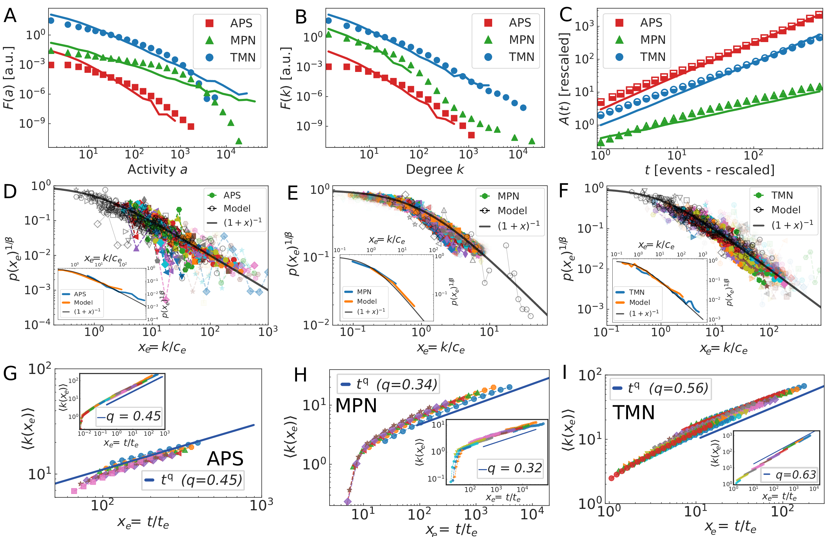
Figure 1: The stylized facts of the three datasets considered in this paper. (A) The $F(a)$ activity distribution, (B) the $F(k)$ degree distribution, and, (C) the temporal growth of the total number of edges $A(t)\propto t^{\gamma}$ as found in the APS (red squares), MPN (green triangles) and TMN (blue circles) datasets. For each case, we also show the corresponding curves, as found in the model best fitting each dataset (solid lines with the same color as the corresponding dataset). The rescaled strengthening probability $p(k)=(1+k/c_{e})^{-\beta}$ as measured for different classes of nodes (symbols, color depth proportional to the number of agents in a node class $e$) is reported in panel (D) for the APS dataset, in (E) for the MPN case, and, in (F) for the TMN system. In the main panels we compare the empirical curves (colored symbols) with the $p_{e}(k)$ found in the corresponding best-fitting urn model (black symbols) and the theoretical guideline $p(x_{e})^{1/\beta}=(1+x_{e})^{-1}$ (black solid lines), being $x_{e}$ the rescaled degree $x_{e}=k/c_{e}$. In the insets we show the average rescaled $\langle p(x_{e})\rangle_{e}$ for the empirical (blue lines) and synthetic data (orange lines) as well as the theoretical behavior $p(x)=(1+x)^{-1}$ (black line). (G-I) Main panels: the average degree $\langle k(t_{e},t)\rangle\propto(t/t_{e})^{q}$ as a function of $x_{e}=t/t_{e}$ for different classes of nodes entering the system at different times $t_{e}$ (colored symbols) for the APS (G), MPN (H), and TMN system (I), respectively. In the insets, we show the corresponding results for the urns model. We also show the best fit $\langle k(x_{e})\rangle\propto x_{e}^{q}$ for all the cases (solid blue lines). Note that here the exponent $q$ does not depend on the class $e$ (refer to SI Section LABEL:sub:si_q_exponent for details).

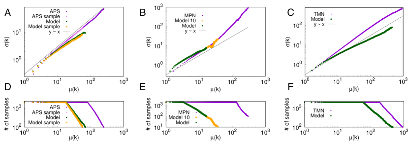
Figure 2: Top. Taylor’s law for the number of links created by different individuals at each (intrinsic) time $t$. We defined $\mu(k)\equiv\langle k(t)\rangle$ and $\sigma(k)\equiv\sqrt{\langle k^{2}(t)\rangle-\langle k(t)\rangle^{2}}$, with implicit dependence on time. Results in the empirical datasets, contrasted with model predictions, for (A) the APS dataset, (B) the MPN dataset, and (C) the TMN dataset. In Fig. (A) we report results also for the 1-link sampled database, defined in the Methods section. For all the empirical and synthetic datasets we find an approximate power-law behavior $\sigma(k)\sim\mu(k)^{\delta}$, with $\delta\gtrsim 1$. For each curve (both for the empirical and synthetic datasets), we considered the $2000$ individuals with the longest history (final intrinsic time). Bottom. We report here the effective number of points on which the mean and the standard deviation is computed at each time $t$. This number decreases for the highest values of the mean, corresponding to higher values of intrinsic time since the number of the total performed actions varies from individual to individual. The number of samples used is reported, both for the empirical and synthetic datasets, for (D) the APS dataset, (E) the MPN dataset, and (F) the TMN dataset. In all the cases, we considered only averages on at least $100$ samples, but for the MPN case, where we additionally show values for times where at least $10$ samples were available (Model 10 curves).

The datasets mentioned above have been extensively studied and characterized in previous works [22, 23, 41, 18], and we resume here their main properties and features. The most renowned property of these systems is that both the propensity of a user to engage in social interaction (i.e., the activity $a_{i}$ of a node $i$ defined as the number of events actively engaged by node $i$) and the degree $k_{i}$ (i.e., the number of different neighbors connected to node $i$) are found to be broadly distributed. The tails of their distributions are usually approximated with a power-law, i.e.,

$$F(a)\propto a^{-(\eta+1)}\quad\text{and}\quad F(k)\propto k^{-\mu},$$

as shown in Fig. 1A-B.

These systems are also expanding in time as new nodes and edges keep entering the network. In Fig. 1C we show the growth in intrinsic time $t$ (i.e., the number of recorded events) of the number of edges $A(t)$ in the systems that follows a Heaps’ law as

$$A(t)\propto t^{\gamma}$$

(see Section LABEL:sec:si_results in the SI for details).

Another key feature of social interactions is that individuals display correlations on their activity. When a node engages a social interaction, it is likely to turn its social activity (e.g., a mention in the TMN) toward a node already contacted in the past rather than toward a randomly selected node in the system. A possible way to quantify this mechanism is to measure the probability $p_{k\to k+1}(k)$ (in short $p(k)$) for a node that already contacted $k$ different nodes to contact a new one the next time it will be active [18, 22]. The $p(k)$, which is formally the probability to pass from degree $k\to k+1$, was found to feature the same functional form

$$p(k)=\left(1+\frac{k}{c}\right)^{-\beta}$$

across all the datasets we here consider [22]. Specifically, it turns out that we can characterize a system through a single value of $\beta$ (the strengthening exponent) and a distribution of values of the strengthening constants $c$. The constant $c$ sets the scale at which an individual decreases his ability to acquire new contacts. At odds with the strengthening exponent $\beta$, $c$ significantly varies across individuals. To further explore this variability, we grouped individuals in different classes, $e$, according to their entrance time $t_{e}$ into the system and their final degree $k_{e}$ (refer to the Methods section). We show in Fig. 1D-F both the $p(x_{e})$, with $x_{e}=k/c_{e}$ for each class $e$, (main panels) and the average value of the rescaled probability $\langle p(x_{e})\rangle_{e}$ (insets), as found in the empirical data and, for comparison, in the synthetic results of our modeling framework (see also methods and SI Section LABEL:sec:si_results for details). This tendency to slow down the creation of new links also reflects in a sub-linear growth of the average degree

$$\langle k(t_{e},t)\rangle\propto t^{q},$$

with $q<1$, as shown in Fig. 1G-I. We further explore for the first time a finer-grained behavior, Taylor’s law [42, 43], recently pointed out as a shared feature in evolving systems, when referred to fluctuations in innovation rate [44, 45]. Taylor’s law relates the standard deviation of a random variable to its mean, and the onset of complex behavior is characterized by

$$\sigma(t)\propto\mu(t)^{\delta}$$

with $\delta\geq 1$, at odds with $\delta=1/2$ characterizing uncorrelated events. A complex behavior of Taylor’s law does not trivially follow from Zipf’s and Heaps’ laws [44, 45], making it a relevant observable to test theoretical predictions. We here measure Taylor’s law referred to the growth of individual connections in the network, observing a linear or superlinear behavior (Fig. 2).

In addition to these global observables, we also track a set of local observables, later presented in the Results section, measuring how agents allocate their events in their local network of contacts, e.g., reinforcing old contacts or establishing new links either closing or not closing existing triangles in the emerging social graph.

In the following, we propose a minimalistic, first-principles model of network evolution that reproduces all the features mentioned above and provides more in-depth insight into the microscopic dynamics shaping the growth and evolution of social networks.

A first-principles model for social networks

We now introduce our first-principles model for the birth and evolution of social networks. The model we propose builds on the expansion of the Adjacent Possible framework [28] to the exploration of social spaces where individuals are embedded. In this framework, we can microscopically model the space of possibilities of a node, i.e., the set of all the social interactions that are "possible" for a node within the social network. This space, at a given point in time, consists of three distinct regions: i) the actual, including all the links already experienced by the individuals in the past (current connections), ii) the adjacent possible comprehending all the links that are just one step away from being explored (e.g., the friends of friends that we still do not know), and, iii) the unknown, accounting for all the links not yet conceivable by the node at present, but that may become adjacent and possible at some later stage.

A second essential ingredient of our modeling scheme concerns the phenomenon of the so-called correlated novelties [28]. Every time the social exploration process of a node $i$ activates a new connection with a node $j$ belonging to its adjacent possible, $i$ and $j$ experience a novelty, i.e., the link $e_{ij}$ gets active for the first time. In this way, $j$ becomes now part of the actual region of $i$ and the adjacent possible of $i$ reacts to this novelty by surrounding it with freshly created adjacent possible, i.e., new possible connections that were not possible for $i$ before. In other words, a novelty paves the way to another in the future.

Model rules

The modeling scheme we apply is a multi-agent version of a modified Polya urn [30, 31] that proved to be able to reproduce the adjacent possible evolution in different contexts. In particular, it was proven to account for the main statistical features shared by complex evolving systems (Zipf’s, Heaps’ and Taylor’s law) and observed correlations in a more sophisticated version [28, 32, 46, 45]. In the simpler formulation of that model [28], the key ingredient is an urn, $\mathcal{U}$, containing $N_{0}$ distinct elements. One may think of them as balls of different colors representing an item of the space being explored. The dynamics proceeds by repeatedly withdraw balls from $\mathcal{U}$ and annotating them in a temporal sequence of events (this sequence may alternatively represent, depending on the context, a sequence of phone calls made, or a list of co-authors of new scientific publications or a sequence of retweets). Every time we pick up a ball, we put it back in the urn together with $\rho$ additional copies of it, thereby reinforcing that element’s likelihood of being drawn again in the future, in a “rich-get-richer” fashion. Also, to account for the adjacent possible expansion, whenever a novel (never extracted before) element appears in the sequence, we additionally put $\nu+1$ new distinct elements in $\mathcal{U}$, thus expanding the adjacent possible of the system.

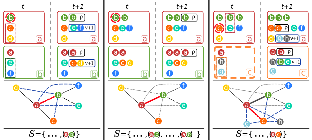
Figure 3: Three possible steps of the Polya’s urn model for a system with $\rho=\nu=1$ with sampling strategy $s=$WSW. For each evolutionary step of the system (columns), we show the current state of the urns (top row), the equivalent network evolution (mid row), and, the sequence $\mathcal{S}$ of observed events (bottom row). In the network, we show already active links (solid lines), links in the adjacent possible (dashed lines), currently active links (red lines) and connections entering into the adjacent possible (blue dashed lines). First column: at time $t$ urn $a$ is active and draws a ball with ID $b$ (red-circled ball): the event $(a,b)$ is then appended to the sequence $\mathcal{S}$. At time $t+1$ the $a$ urns then gains $\rho$ copies of $b$ and vice-versa (reinforcement) and, since the $e_{ab}$ link is new, we also draw $\nu+1$ distinct balls from $a$ following the WSW strategy (balls $c$ and $d$ within dashed rectangle) that will be copied into $b$ (and the same for $b$ that sends $e$ and $f$ as novelties to $a$). Mid row: the $e_{ab}$ edge is active and the $e_{ae},\,e_{af},\,e_{bc}$ and $e_{bd}$ links enters into the adjacent possible. Notice that the adjacent possible of $c$ changed without the need for $c$ to participate in a social interaction. Second column: at time $t$, urn $a$ draws a copy of $b$ (top). Since the edge $e_{ab}$ was already active in the past, we only put $\rho$ copies of $b$ in urn $a$ and the other way around. The network’s topology does not change in this step, while the weight of the $e_{ab}$ link gets increased (mid row). Third column: urn $a$ draws a copy of $c$ at time $t$ (top). Since $c$ is an empty urn, it creates $\nu+1$ novel IDs ($g$ and $h$, in the dashed rectangle) and gains a copy of them. We add $(a,c)$ to the sequence $\mathcal{S}$ and we perform the reinforcement/novelties exchange between $a$ and $c$. The network gains two new nodes ($g$ and $h$), activates a new edge ($e_{ac}$) and inserts new links in the adjacent possible. The actual space of $c$ acquires $a$ while its adjacent possible gains $e,\,g$, and $h$.

To account for the birth and evolution of social networks, we generalize this model to a multi-agent version. The paradigmatic shift is twofold. On the one hand, the system will consist of a collection of urns, each identified by a unique alphanumeric ID ($a,b,c,\ldots$), representing users in a social network. On the other hand, each ball within each urn will bear the reference ID of another urn in the system. Then, the sequence of extracted balls will be the series of social contacts annotated as tuples $(i,j)$, where $i$ is the ID of the urn drawing a ball, and $j$ is the ID of the drawn ball. For each extraction, the reinforcement process requires to put back $\rho$ copies of the extracted ball $j$ into the extracting urn $i$ (and vice versa), so that an exploited interaction will be favored again in the future. To account for the expansion of the adjacent possible, we also let two urns that interact for the first time to exchange a memory buffer, i.e., a subset of $\nu+1$ balls each urn that is reciprocally shared. Thanks to this exchange, an urn that experiences a novelty, i.e., that establishes a connection never explored before, expands its adjacent possible —i.e., the set of IDs that it may contact in the future. A schematic representation of the model is given in Fig. 3 and we resume here the steps defining it (see the methods section and the SI Section LABEL:sec:si_model for further details):

1. we start with two urns, $a$ and $b$ having a copy of each other’s ID inside of them; the urns also contain the $\nu+1$ distinct identities (IDs) of other urns that did not participate yet to any interaction ($c$, $d$ for $a$ and $e$, $f$ for $b$). This set is their memory buffer at the initial stage. We shall come back later on the different strategies to update it during the evolution of the system. The sequence of events $\mathcal{S}$ is initially empty;

2. at each time step, we extract a “calling” urn $i$ with probability proportional to the size of the urn $U_{i}$ (the number of balls within the urn $i$). We then draw a ball from the calling urn $i$, say the ID $j$. This double extraction corresponds to a single event $(i,j)$ that we append to the main sequence $\mathcal{S}$. In Fig. 3 the first event is the $(a,b)$ one.

3. reinforcement: following the event $(i,j)$, we add $\rho$ copies of $i$ in the $j$’s urn and $\rho$ copies of $j$ in the $i$’s urn. For example, in the first column of Fig. 3, we add $\rho$ copies of $a$ in the $b$’s urn and $\rho$ copies of $b$ in the $a$’s urn.

4. novelty: if it is the first time that $i$ and $j$ interact, $i$ and $j$ exchange their memory buffer. With this mechanism, we add $j$’s memory buffer into $U_{i}$ and, vice-versa, $i$’s memory buffer into $U_{j}$. In Fig. 3, first column, $a$’s memory buffer ($c$, $d$) is copied into $U_{b}$ and $b$’s memory buffer ($e$, $f$) is copied into $U_{a}$.

5. if a node $j$ is called for the first time by another node (i.e., $j$ is an empty urn so that $U_{j}=0$), it creates $\nu+1$ new agents (empty urns) and, for each of them it creates a ball into its urn: these $\nu+1$ IDs represent the initial memory buffer of $j$. In Fig. 3 (third column) node $c$ creates two brand new nodes, $g$ and $h$, that will represent its initial memory buffer. We note here that the newly created agents are initially empty urns so that they can participate in the dynamics (they can be included in the social network) only if another urn (agent) calls them. Only after this first call, they become active. In this scheme, an agent cannot join the network "from outside," i.e., unless it is engaged by another agent already belonging to the network. Of course, the scheme can be generalized to include a sort of "immigration," but this aspect will not be discussed in the present work.

Each evolution step is defined as a repetition of the $2\to 5$ steps of the just outlined procedure, as shown in Fig. 3. The parameters $\rho$ and $\nu$ weigh the relative importance of the reinforcement and exploration processes in the system. We define $R=\rho/\nu$ as the ratio between the two.

Sharing of past experiences

The last ingredient of our modeling scheme is the strategy that an agent adopts when sharing its experience (the memory buffer) with nodes encountered for the first time. To this end, we introduce different strategies $s$ to determine the $\nu+1$ IDs contained in the memory buffer being shared along with new links. Here, we report three of these strategies that turn out to best capture the phenomenology of the empirical datasets we consider, while we refer to the SI Section LABEL:sec:si_model for additional strategies. (i) Weighted Sample with Withdrawal (WSW) strategy: an agent draws $\nu+1$ distinct IDs from the urn proportionally to their abundance in the urn itself at that time, i.e., proportional to the number of the past interactions with each ID. This strategy corresponds to sharing the IDs that interacted the most with a node in the past and is the one applied in Fig. 3; (ii) Symmetric Sliding Window (SSW): each agent keeps a buffer of its last $\nu+1$ interactions that represent the list of IDs shared with a newly contacted agent. After the exchange, both agents update their memory buffer by pushing in the ID of the agent just contacted and removing the $\nu+1$-th ID from their buffers. This strategy favors the spreading in the network of the recently activated connections, rather than the most frequent ones; (iii) Asymmetric Sliding Window (ASW): it is a variant of the previous one, where only the agent that initiated the interaction updates its memory buffer after the communication event.

The model is then entirely defined by three parameters only: the reinforcement value $\rho$, the ratio $R=\rho/\nu$ setting the relative importance of the reinforcement (exploit) and novelties (explore) mechanisms, and strategy $s$ used to exchange the memory buffer between nodes getting in contact for the first time.

Results

In this section, we report the main features emerging from our modeling scheme’s evolution and compare them to the empirical data of the three real-life social networks we previously introduced. To better compare the theoretical predictions with the observed data, we optimized the model by fixing the parameter values to maximize, for each empirical dataset, a score function $S_{d}(\rho,R,s)$. It evaluates the goodness of fit of the synthetic simulations to the empirical dataset $d$ by looking at eight selected observables, both local and global, static and dynamic (see the methods section for details). We consider in particular the exponents of the power laws discussed in section Stylized facts about social networks, as well as topological measures: (i) the average clustering coefficient, (ii) the fraction of newly created edges that are either old (already activated in the past), new (being activated now) and that happen to close a triangle (closed) or not (open). We create thus four categories: the old open (OO), the old closed (OC), new open (NO) and new closed (NC), and measure the fraction of events falling in each category per time range in the asymptotic limit of the system evolution (see also the methods section). We summarize the results in radar plots in Fig. 4, showing the observed values for the eight selected observables along with the best theoretical estimates. We observe that the model endowed with optimal values of the parameters is able to reproduce all the selected observables in all the datasets quantitatively, but the APS dataset, where the model fails to predict the observables related to the network topology correctly. To explain this discrepancy, we note that the APS dataset is composed of cliques of events —rather than one single event between two ids per time. This feature leads to a naturally significant clustering coefficient (as all the agents publishing one paper are fully connected) and in an increased count of events observed along old edges insisting on at least one closed triangle. To filter out this effect, we performed a sub-sampling of the data by drawing a single link among all the possible ones for each paper and re-computed the features of this sub-sampled dataset (see the methods section and the SI Section LABEL:sec:si_APS_subsample for further sampling strategies). In this way, the disagreement between the real system and the model results disappears (see Fig. 4(A)), revealing that the model can explain the underlying interaction processes also in this dataset.

In the SI, we additionally show how the model parameters affect the main observables of the system. Here we say that, as for the global observables discussed in section Stylized facts about social networks and reported in Fig. 1 and Fig. 2, the relevant parameters are the ratio $R=\rho/\nu$ and the sharing strategy $s$, while the absolute values of $\rho$ and $\nu$ impact the behavior of the observables related to the local topology of the network. Despite the limited number of parameters, the model is flexible enough to reproduce a wide range of phenomenologies, from highly exploratory situations (high $\gamma$ and $\beta$ exponents) to more exploitative scenarios, with a reduced number of connections being explored.

Global trends

To make contact with real-world social networks, in Fig. 1, we contrast the synthetic results with the empirical datasets considered. Specifically, we show that the model can reproduce broad activity (A) and degree distributions (B), the time evolution of the number of edges in the network $E(t)\propto t^{\gamma}$ (C), the functional form of the strengthening function $p(k)$ (D-F), as well as the sub-linear growth in of the average degree (G-I). Further, the model can reproduce the broad fluctuations in the rate of innovation (i.e., in the creation of new links), as measured by Taylor’s law (Fig. 2). All these observables are discussed in section Stylized facts about social networks.

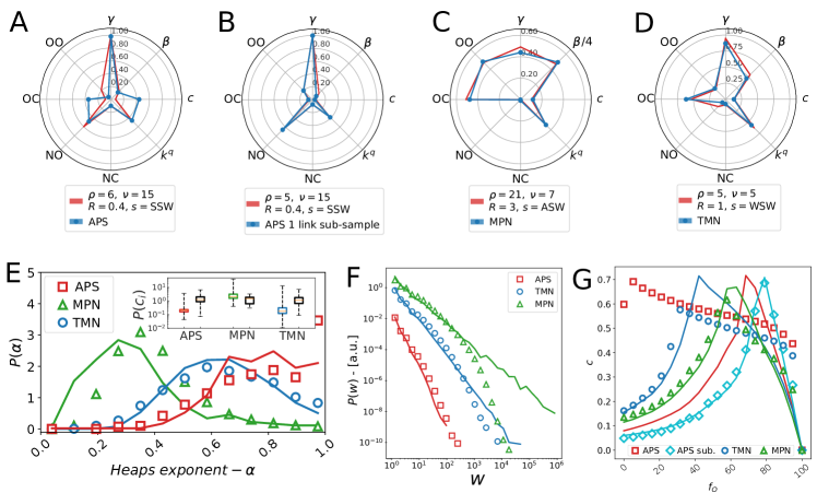
Figure 4: (A-D) Radar plots comparing eight selected observables measured in empirical and synthetic data. For each dataset, we show the observed values (blue lines) and the corresponding values in the synthetic model fitting (red lines). For each fitting model, we report the reinforcement and novelties parameters $\rho$ and $\nu$ and their ratio $R$ as well as the optimal sampling strategy $s$. (E) The distribution of the local Heaps’ exponent $\alpha$ for a sample of $10\%$ of nodes as measured in the empirical datasets (symbols) and the synthetic simulations (solid lines) for the APS (red), MPN (green), and TMN (blue) datasets. In the inset, we show the distribution of the strengthening constant $c_{i}$ as measured in data (colored boxes) and corresponding simulations (black boxes). (F) The $P(w)$ link weight distribution for the three empirical datasets (symbols) and the ones found in the artificial networks (solid lines). (G) The average clustering coefficient $c(f_{O})$ as a function of the fraction of removed edges with overlap $O\leq f_{O}$. Symbols refer to empirical data, while solid lines represent the synthetic results (the cyan color is used for the $1$-link sampling of APS).

We summarize the results in radar plots in Fig. 4, showing the observed values for the eight selected observables along with the best theoretical estimates. With these parameters’ values, we compare the model predictions with empirical findings for different local observables.

Heterogeneities in the experience of the new

Interestingly, the model also correctly captures the heterogeneous propensity of individuals to establish new connections, i.e., the rate at which they experience novelties. To quantify this rate, we look at the exponent of the Heaps’ law describing the growth of the degree of an individual, $k_{i}(x_{i})$, i.e., the number of distinct people encountered as a function of the number of social events performed $x_{i}$: $k_{i}(x_{i})\propto x_{i}^{\alpha}$. Fig. 4(E) reports the distribution of empirical exponents $\alpha$ for the three datasets considered. These distributions are peaked at different $\bar{\alpha}_{d}$ values for the different datasets ($\bar{\alpha}_{\rm APS}\sim 0.9$, while $\bar{\alpha}_{\rm TMN}\sim 0.7$ and $\bar{\alpha}_{\rm MPN}\sim 0.4$). We also report the $P(\alpha)$ distributions as obtained using our modeling scheme. Remarkably, the model correctly reproduces both the peak value and the broadness of each empirical $P(\alpha)$ distribution.

Another signature of heterogeneity in the empirical data is represented by the distribution of the strengthening constants $c_{i}$. We remind that the constants $c_{i}$ enter the probability for an individual with $k$ connections to acquire a new one:

$$p_{i}(k)=(1+k/c_{i})^{-\beta},$$

where the coefficient $c_{i}$ modulates the propensity of individual $i$ to create new connections. The inset of Fig. 4E illustrates how our modeling scheme qualitatively reproduces the empirical $P(c_{i})$ of the strengthening constants $c_{i}$. This is another important result, already anticipated in Fig. 1, as the model synthetically reproduces the different propensity of individuals in a social network to decrease their social exploration at a given cumulative $k$.

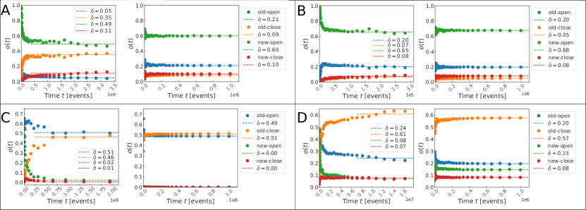
Figure 5: Plot of the empirical data (left column in each panel) and model results (right column in each panel) results for $OO(t)$ (blue markers), $OC(t)$ (orange markers), $NO(t)$ (green markers), and $NC(t)$ (red markers). In each case, we show the temporal behavior (markers), and the asymptotic value (dashed lines, the asymptotic value reported in the legends on the right of the panel). Panels refer to (A) APS, (B) $1$-link subsampling of APS, (C) the MPN dataset, and (D) the TMN dataset.

Topological correlations

We further expand the comparison between empirical and synthetic data checking the topological correlations of the weighted network of interactions among individuals. First, the model correctly reproduces the overall link weight distribution $P(w_{ij})$, i.e., the distribution of the number of activations of a single edge $w_{ij}$ (Fig. 4F). We finally observe that both the empirical and the synthetic data obey the weak and strong ties scheme of the Granovetter conjecture [2, 10, 23]. The latter states that links in a social system will be arranged to have communities of individuals tightly connected by strong ties and with a large neighbors overlap. These communities are then interacting through weak ties, i.e., links acting as bridges between communities between nodes sharing a limited number of common neighbors (low overlap). To prove this, we measure how the average clustering coefficient $c(f_{O})$ of the network varies by removing edges by their ascending overlap $O_{ij}$, i.e., the fraction of common neighbors between nodes $i$ and $j$ (see Methods section for details). In Fig. 4(G), we plot the average clustering coefficient $c(f_{O})$ computed in a network where we remove all the edges $e_{ij}$ with overlap $O_{ij}\leq f_{O}$, being $f_{O}$ the percentile of the overlap distribution. We find $c(f_{O})$ to increase as one removes edges with small overlap (indicating that the removal of weak ties is removing bridges between communities) until the $c(f_{O})$ peaks. After the maximum, if we keep removing the higher overlap edges, we start breaking the triangles in the communities’ cores, and the clustering coefficient decreases. The APS dataset is found to be in disagreement with synthetic data. As already noted above, this disagreement can be explained, remembering that in these datasets, events are composed of cliques of interacting authors, whereas the model only accounts for pairwise interactions. To filter out this difference, we repeated the clustering measure vs. overlap curve on the $1$-link sub-sampled APS dataset. The result is reported in Fig. 4(G), showing a perfect agreement between the model and the data.

As a last measure to investigate the agreement between the model predictions and empirical findings on the microscopic dynamics, we report the temporal evolution of the number of events allocating toward new or old links insisting or not on triangles (the categories $OO$, $OC$, $NO$, and $NC$ defined above and in the methods section). Again, we note that, while the original dataset APS shows a behavior not well reproduced by the model, the latter very nicely predicts the behavior featured by the $1$-link sub-sampled APS dataset, as well as the behavior shown by the other two datasets (Fig. 5).

Exploration strategies

Let us finally note that the parameter configuration found to describe better each dataset draws some meaningful insights on the microscopic mechanisms driving the exploration of the social space at the individual level. In the TMN case, we find $R=1$, so that the reinforcement and the novelty exchange processes equally influence the single agents’ exploration process: this is reasonable in a system where new connections require little effort from the user. Moreover, the strategy $s=$WSW with $\nu=5$ is the one that better describes the empirical data: users select new accounts to follow by sampling from the past interactions of the alters they are connecting with proportionally to their popularity.

On the other hand, in the MPN case, the best fit is obtained for $R=3$ and $\rho=21$. The system dynamic is dominated by reinforcement processes that tend to reinforce links that are first established and inhibiting the creation of new edges. In this case, the best fit with the $s=$ASW memory buffer sampling strategy highlights that individuals share their last $\nu+1=8$ contacts, thus spreading copies of recently contacted IDs rather than the most contacted ones. Notice that the last contacted $\nu+1$ IDs may, in general, be different from the most representative IDs within the urn. The asymmetric nature of the ASW strategy indicates that users actively exploring new connections update their memory buffer, whereas nodes passively participating in communication tend to conserve their previous memory buffers.

Finally, in the APS case, we find an extremely exploratory dynamics characterized by a relatively low $R=0.4$, i.e., a relatively high $\nu$. This finding is symptomatic of a dynamics where the exploration of the social space overtakes the reinforcement of existing connections. A possible explanation lies in many students and researchers authoring a few papers before quitting academia and research, providing a constant influx of new potential connections to be explored by senior researchers. The $SSW$ optimal sampling strategy reveals that authors tend to share their last $\nu+1\simeq 16$ people they have been collaborating with, implying a preference to recommend recently active connections to new collaborators. Moreover, this strategy also catches the intrinsic symmetric nature of the co-authorship interaction, as both co-authors update their buffers of potential new collaborators.

Discussion

In this work, we proposed a first-principles theoretical model of social exploration to explain the birth and evolution of social networks. The theory is based on the notion of Adjacent Possible and builds on a recently introduced mathematical formalization of its conditional expansion. In this framework, the creation of new social bonds is the outcome of an exploration process unfolding on the space of possible new acquaintances, whose boundaries change while people explore them.

Without relying on unnecessary assumptions, our new theory starts from first principles and predicts both microscopic and macroscopic features of real-world social networks. We compared the predictions with the empirical data from three diverse social networks: the system of Twitter users, the network of co-authorship of the American Physical Society, and the phone-call network. The agreement between theory and data is surprisingly good. On the macroscopic side, the model reproduces the main static and dynamic features of those social networks: the broad distribution of degree and activities, the average clustering coefficient, and the innovation rate at the global and local levels. At the microscopic level, the most striking feature captured is the probability for an individual, with already $k$ connections in its local network, to acquire a new acquaintance. The model also captures topological correlations and the dynamics of real-world systems at very different scales, from the local exploit/explore mechanisms of single agents to the global organization of the network in communities of coherent users.

Besides being able to capture very complex features of social networks quantitatively, our theory also allows us to deepen our understanding of the microscopic mechanisms shaping the propensity of people to reinforce old contacts or establish new ones. For instance, in Twitter mentions network, we find the exploration and reinforcement processes to be of equal importance. Moreover, when getting in contact with new alters, users share a sample of their most common contacts as new potential connections. On the other end of the spectrum, in the mobile phone-calls network, people reinforce their existing bonds more than explore new ones. When suggesting new potential contacts to others, people tend to exchange their most recent contacts, rather than their most common ones. Finally, the network of scientific co-authorship of the American Physical Society journals features the most exploratory dynamics, with new connections massively expanding the adjacent possible of a single node. In this case, people preferably share their last contacts, and the optimal synthetic update procedure is symmetrical, correctly reproducing the intrinsic symmetric nature of the interactions.

The theoretical framework proposed here is, of course, open to possible improvements. First, the simulated dynamics describes the evolution of a system from its outset. The initial conditions set here could be far from those of the real-world systems considered. Despite the excellent agreement with empirical data, a more comprehensive study on the dependence of the system evolution on the initial state is in order. Other generalizations could concern the possibility to remove links or to decouple the rate of addition of links from the that of the entrance of new nodes. Finally, our modeling scheme does not account for effects connected to semantics or affinity between people. For instance, it seems reasonable to assume that people create bonds and interact based on shared interests or their level of homophily. The generality of the approach presented here will make the extension of the theoretical framework desirable and possible along these lines.

Nevertheless, we believe that the presented framework, together with its predictions validated on real-world social networks, represents a fundamental step toward understanding the processes underlying the birth and evolution of social networks. It further creates an important bridge between network theory and urns models, opening the way to constructive contamination between the two fields and a full exploitation of results derived for stochastic processes relevant in innovation dynamics [47, 46, 45]. This development, in turn, unlocks the possibility to grasp the very essence of social interactions and allows for the design of efficient and informed policies to address crucial challenges dealing with collective processes ongoing in social networks, such as the spread of diseases and online misinformation.

Contributions

All authors conceived and designed the research work. EU ran the simulations and analyzed the data. All authors wrote and reviewed the article.

Author declarations

The authors declare no conflict of interest.

Acknowledgement

The authors would like to thank M. Karsai for useful comments and for granting us access to the mobile phone dataset and V.D.P. Servedio for inspiring discussions and relevant suggestions.

Materials and Methods

Data and code

The three datasets used in the study are:

• The co-authorship networks found in the Journals of the American Physical Society [38] covering the period between Jan. $1970$ to Dec. $2006$ and containing $301,236$ papers written by $184,583$ authors that are connected by $995,904$ edges.

• Twitter Mentions Network (TMN), containing all the mention events exchanged by users from January to September $2008$. The network has $536,210$ nodes performing about $160$M events and connected by $2.6$M edges;

• Mobile Phone calls Network (MPN) composed of $6,779,063$ users of a single operator with about $20$% market share in an undisclosed European country from January to July $2008$. The datasets contain all the phone calls to and from company users, thus including the calls towards or from $33,160,589$ users in the country connected by $92,784,825$ edges.

• The synthetic simulations have been run for $T=10^{6}$ evolution steps for configurations with $R\leq 1$, $T=5\cdot 10^{7}$ otherwise.

The code used to run the simulations, all the analysis code, as well as the synthetic data analyzed, are available in [48]. Due to data policies and IPR, we cannot share the MPN and TMN data, while the APS data are from the work in [38].

Asymptotic behavior of the system

In this work, we leverage on a previous analysis performed on the same datasets as found in  [22]. Specifically, we measure the strengthening probability $p(k)$, i.e., the probability for an individual who already contacted $k$ distinct individuals in the past to contact a new one (i.e., a new node of the network). To average this probability on homogeneous classes of people, we divide the nodes in $g=1,\ldots,G$ classes depending on their time of entrance in the system, $t_{e}$, and their final degree $k_{e}$, one class for each combination of $t_{e}$ and $k_{e}$. The functional form of the probability $p(k)$ is found to depend on the class $e$ of the nodes as $p(k_{e})=(1+k/c_{e})^{-\beta}$ with a single overall $\beta$ exponent and a distributed reinforcement constant $c_{e}$. As for the growth of the average degree $\langle k(t_{e},t)\rangle$, we measure the average degree at time $t>t_{e}$ for all the nodes belonging to the class with entrance time $t_{e}$. In this way, we are defining a new set of classes only defined in terms of the entrance time $t_{e}$. The asymptotic behavior is found to be $\langle k(t_{e},t)\rangle\propto t^{q}$.

Model score

We ran the model at different values of $R$ and $\rho$ for each one of the six sample strategies $s$ (see SI Section LABEL:sec:si_results for details). For each dataset $d$ we select the configuration that best fit the data by looking at the score $S_{d}(\rho,R,s)$ that reads

$$S^{d}(\rho,R,s)=\sum_{i=1}^{8}{\frac{|o^{d}_{i}-\tilde{o_{i}}(\rho,R,s)|}{\sigma^{d}_{i}}},$$ (1)

where $o^{d}_{i}$ and $\sigma^{d}_{i}$ are the value and uncertainty on the $i$-th observable of the empirical dataset and $\tilde{o_{i}}(\rho,R,s)$ is the value of the same observable measured in the simulations with configuration $(\rho,R,s)$. The eight selected observables are: 1) the exponent $\gamma$ leading the growth of the number of edges $E(t)\propto t^{\gamma}$, 2) the optimal $\beta$ measured in the strengthening function $p(k)$, 3) the average clustering coefficient $c$, 4) the exponent leading the growth of the average degree per node class $\langle k(e,t)\rangle\propto t^{q}$, 4-8) the fractions $OO$, $OC$, $NO$, $NC$ of events allocated toward old/new link insisting or not on a open/closed triangle (see SI Section LABEL:sec:si_results for details).

APS subsampling

In the APS dataset we transform each paper published by $n$ authors in a sequence of $E=n(n-1)$ events with all the possible links between all the ordered couples of co-authors. We then sample $l$ links over the $E$ possible links for each paper to be inserted in the total sequence $\mathcal{S}$. The results reported in the main text refer to $l=1$, and the reader can refer to the SI Section LABEL:sec:si_APS_subsample for results with different values of $l$ and different strategies of subsampling (number of sampled links proportional to $E$).

Events on new-old and open-closed edges

We count, for each logarithmically spaced time interval, the number of events happening on edges that are either old (already activated in the past), new (being activated now) and that happen to close a triangle (closed) or not (open). These four categories are then: the old open ($OO$), the old closed ($OC$), new open ($NO$) and new closed ($NC$) that we define as the fraction of events falling in each category per time range in the asymptotic limit of the system evolution —i.e., after 60% of the events passed.

References

- [1] Matteo Marsili, Fernando Vega-Redondo, and František Slanina. The rise and fall of a networked society: A formal model. Proceedings of the National Academy of Sciences, 101(6):1439–1442, 2004.
- [2] M. Granovetter. Getting a Job: A Study of Contacts and Careers. Sociology (University of Chicago Press). University of Chicago Press, 1995.
- [3] Vedran Sekara, Arkadiusz Stopczynski, and Sune Lehmann. Fundamental structures of dynamic social networks. Proceedings of the National Academy of Sciences, 113(36):9977–9982, 2016.
- [4] Gueorgi Kossinets and Duncan J Watts. Empirical analysis of an evolving social network. science, 311(5757):88–90, 2006.
- [5] Jörn Davidsen, Holger Ebel, and Stefan Bornholdt. Emergence of a small world from local interactions: Modeling acquaintance networks. Physical Review Letters, 88(12):128701, 2002.
- [6] Emily M. Jin, Michelle Girvan, and M. E. J. Newman. Structure of growing social networks. Phys. Rev. E, 64:046132, Sep 2001.
- [7] J.-P. Onnela, J. Saramäki, J. Hyvönen, G. Szabó, D. Lazer, K. Kaski, J. Kertész, and A.-L. Barabási. Structure and tie strengths in mobile communication networks. Proceedings of the National Academy of Sciences, 104(18):7332–7336, 2007.
- [8] Janos M Kumpula, J-P Onnela, Jari Saramäki, Janos Kertész, and Kimmo Kaski. Model of community emergence in weighted social networks. Computer Physics Communications, 180(4):517–522, 2009.
- [9] Janos M Kumpula, J-P Onnela, Jari Saramäki, Janos Kertész, and Kimmo Kaski. Model of community emergence in weighted social networks. Computer Physics Communications, 180(4):517–522, 2009.
- [10] Mark S Granovetter. The strength of weak ties. In Social networks, pages 347–367. Elsevier, 1977.
- [11] Petter Holme and Jari Saramäki. Temporal networks. Physics reports, 519(3):97–125, 2012.
- [12] Nicola Perra, Bruno Gonçalves, Romualdo Pastor-Satorras, and Alessandro Vespignani. Activity driven modeling of time varying networks. Scientific reports, 2:469, 2012.
- [13] Giovanna Miritello, Rubén Lara, Manuel Cebrian, and Esteban Moro. Limited communication capacity unveils strategies for human interaction. Scientific reports, 3:1950, 2013.
- [14] Giovanna Miritello, Esteban Moro, and Rubén Lara. Dynamical strength of social ties in information spreading. Physical Review E, 83(4):045102, 2011.
- [15] Antoine Moinet, Michele Starnini, and Romualdo Pastor-Satorras. Burstiness and aging in social temporal networks. Physical review letters, 114(10):108701, 2015.
- [16] Christian L Vestergaard, Mathieu Génois, and Alain Barrat. How memory generates heterogeneous dynamics in temporal networks. Physical Review E, 90(4):042805, 2014.
- [17] Alain Barrat, Marc Barthlemy, and Alessandro Vespignani. Dynamical Processes on Complex Networks. Cambridge University Press, New York, NY, USA, 1st edition, 2008.
- [18] Marton Karsai, Nicola Perra, and Alessandro Vespignani. Time varying networks and the weakness of strong ties. Sci. Rep., 4:4001, 02 2014.
- [19] Márton Karsai, Mikko Kivelä, Raj Kumar Pan, Kimmo Kaski, János Kertész, A-L Barabási, and Jari Saramäki. Small but slow world: How network topology and burstiness slow down spreading. Physical Review E, 83(2):025102, 2011.
- [20] Enrico Ubaldi, Alessandro Vezzani, Márton Karsai, Nicola Perra, and Raffaella Burioni. Burstiness and tie activation strategies in time-varying social networks. Scientific reports, 7:46225, 2017.
- [21] Alain Barrat, Bastien Fernandez, Kevin K Lin, and Lai-Sang Young. Modeling temporal networks using random itineraries. Physical review letters, 110(15):158702, 2013.
- [22] Enrico Ubaldi, Nicola Perra, Márton Karsai, Alessandro Vezzani, Raffaella Burioni, and Alessandro Vespignani. Asymptotic theory of time-varying social networks with heterogeneous activity and tie allocation. Scientific Reports, 6:35724 EP –, 10 2016.
- [23] Guillaume Laurent, Jari Saramäki, and Márton Karsai. From calls to communities: a model for time-varying social networks. The European Physical Journal B, 88(11):1–10, 2015.
- [24] Ciro Cattuto, Alain Barrat, Andrea Baldassarri, Gregory Schehr, and Vittorio Loreto. Collective dynamics of social annotation. Proceedings of the National Academy of Sciences, 106(26):10511–10515, 2009.
- [25] S.A. Kauffman. The Origins of Order: Self-organization and Selection in Evolution. The Origins of Order: Self Organization and Selection in Evolution. Oxford University Press, 1993.
- [26] S.A. Kauffman and N.M.) Santa Fe Institute (Santa Fe. Investigations: The Nature of Autonomous Agents and the Worlds They Mutually Create. SFI working papers. Santa Fe Institute, 1996.
- [27] Stuart A Kauffman. Investigations. Oxford University Press, 2000.
- [28] Francesca Tria, Vittorio Loreto, Vito Domenico Pietro Servedio, and Steven H Strogatz. The dynamics of correlated novelties. Scientific reports, 4:5890, 2014.
- [29] Vittorio Loreto, Vito D. P. Servedio, Steven H. Strogatz, and Francesca Tria. Dynamics on Expanding Spaces: Modeling the Emergence of Novelties, pages 59–83. Springer International Publishing, Cham, 2016.
- [30] George Pólya. Sur quelques points de la théorie des probabilités. Ann. Inst. H. Poincaré, 1(2):117–161, 1930.
- [31] Hosam Mahmoud. Pólya urn models. Chapman and Hall/CRC, 2008.
- [32] Bernardo Monechi, Alvaro Ruiz-Serrano, Francesca Tria, and Vittorio Loreto. Waves of novelties in the expansion into the adjacent possible. PLOS ONE, 12(6):1–18, 06 2017.
- [33] Iacopo Iacopini, Sta ša Milojević, and Vito Latora. Network dynamics of innovation processes. Phys. Rev. Lett., 120:048301, Jan 2018.
- [34] Fabio Saracco, Riccardo Di Clemente, Andrea Gabrielli, and Luciano Pietronero. From innovation to diversification: a simple competitive model. PloS one, 10(11):e0140420, 2015.
- [35] Mark EJ Newman. The structure of scientific collaboration networks. Proceedings of the national academy of sciences, 98(2):404–409, 2001.
- [36] Mark EJ Newman. Scientific collaboration networks. i. network construction and fundamental results. Physical review E, 64(1):016131, 2001.
- [37] Mark EJ Newman. Scientific collaboration networks. ii. shortest paths, weighted networks, and centrality. Physical review E, 64(1):016132, 2001.
- [38] Filippo Radicchi, Santo Fortunato, Benjamin Markines, and Alessandro Vespignani. Diffusion of scientific credits and the ranking of scientists. Phys. Rev. E, 80:056103, Nov 2009.
- [39] Bruno Gonçalves, Nicola Perra, and Alessandro Vespignani. Modeling users’ activity on twitter networks: Validation of dunbar’s number. PloS one, 6(8):e22656, 2011.
- [40] Bufferapp, how twitter evolved from 2006 to 2011. https://blog.bufferapp.com/how-twitter-evolved-from-2006-to-2011, 2016. Accessed: 2018-12-01.
- [41] Hang-Hyun Jo, Márton Karsai, János Kertész, and Kimmo Kaski. Circadian pattern and burstiness in mobile phone communication. New Journal of Physics, 14(1):013055, 2012.
- [42] L. Taylor. Aggregation, variance and the mean. Nature, 189:732, 1961.
- [43] Zoltán Eisler, Imre Bartos, and János Kertész. Fluctuation scaling in complex systems: Taylor’s law and beyond. Advances in Physics, 57(1):89–142, 2008.
- [44] Martin Gerlach and Eduardo G Altmann. Scaling laws and fluctuations in the statistics of word frequencies. New Journal of Physics, 16(11):113010, 2014.
- [45] Francesca Tria, Irene Crimaldi, Giacomo Aletti, and Vito D. P. Servedio. Taylor’s law in innovation processes. Entropy, 22(5), 2020.
- [46] Francesca Tria, Vittorio Loreto, and Vito D. P. Servedio. Zipf’s, heaps’ and taylor’s laws are determined by the expansion into the adjacent possible. Entropy, 20(10), 2018.
- [47] J Pitman. Combinatorial Stochastic Processes. Ecole d’Eté de Probabilités de Saint-Flour XXXII. Springer, 2002.
- [48] Enrico Ubaldi. pyurns. https://github.com/ubi15/pyUrns, 2019.