Probabilistic performance estimators for computational chemistry methods: Systematic Improvement Probability and Ranking Probability Matrix. I. Theory

Abstract

The comparison of benchmark error sets is an essential tool for the evaluation of theories in computational chemistry. The standard ranking of methods by their Mean Unsigned Error is unsatisfactory for several reasons linked to the non-normality of the error distributions and the presence of underlying trends. Complementary statistics have recently been proposed to palliate such deficiencies, such as quantiles of the absolute errors distribution or the mean prediction uncertainty. We introduce here a new score, the systematic improvement probability (SIP), based on the direct system-wise comparison of absolute errors. Independently of the chosen scoring rule, the uncertainty of the statistics due to the incompleteness of the benchmark data sets is also generally overlooked. However, this uncertainty is essential to appreciate the robustness of rankings. In the present article, we develop two indicators based on robust statistics to address this problem: $P_{inv}$, the inversion probability between two values of a statistic, and $\mathbf{P}_{r}$, the ranking probability matrix. We demonstrate also the essential contribution of the correlations between error sets in these scores comparisons.

I Introduction

Benchmarks are a central tool for the evaluation of new theories/methods in quantum chemistry (Mata2017, ). Amongst many possible metrics (Civalleri2012, ), the most common benchmarking statistics are the mean unsigned error (MUE/MAD/MAE…), mean signed error (MSE), root mean squared error (RMSE) and root mean squared deviation (RMSD). The explicit definition of these scores is given in a previous article (Pernot2018, ). In a vast majority of benchmark studies, the MUE, or some variant of it, is used to compare methods performance. Recently (Pernot2018, ), we proposed a more informative probabilistic score, the 95th percentile of the absolute errors distribution ($Q_{95}$).

Whichever the statistic used, the question remains of the robustness of such scores and rankings with respect to the choice of the reference dataset. One easily conceives that the values of these statistics change unpredictably when one adds or removes points in the dataset. Benchmarks implicitly assume that the error sets are representative samples of unknown distributions characterizing model errors for each method – the more systems in the dataset, the best the approximation of the underlying distributions. The quest for large datasets incurs heavy computer charges to perform benchmarks, and there is also a trend to reduce this burden by looking for small, optimally representative, datasets (Gould2018, ; Morgante2019, ). Besides, there are several properties for which the reference data are rather sparse, leading to rather small datasets. Another trend, enhanced by the development of machine learning is to replace experimental values by gold standard calculations, with limitations on the size of accessible systems (Ramakrishnan2015, ; Zaspel2019, ). As the estimated values of the statistics and their uncertainties depend on the size of the dataset, it is important to assess this size effect and its impact on statistics comparison and ranking.

This question has been considered recently by Proppe and Reiher (Proppe2017, ), who used bootstrapping to assess the impact of dataset size and reference data uncertainty on the first place in an intercomparison of Mössbauer isomer shifts estimated by a dozen of DFAs. They concluded that for their dataset of $N=39$ values, at least three methods were competing for the first place, with a slight probabilistic advantage for PBE0. This is a very interesting contribution to the quality assessment of benchmarking tools. We recently considered another approach to this problem by defining an inversion probability $P_{inv}$ for the ranking of two methods (Pernot2018, ). Our definition, which was based on the assumption of a normal distribution of statistics differences and neglected error sets correlations, deserves a more general setup.

In the present study, we revisit the ranking uncertainty problem along several complementary lines:

1. we consider the statistical significance of the difference between two values of a statistic: it depends both on the uncertainty on the estimated values, which is notably influenced by the dataset size, and on the correlation between these values, which is due in a large part to the use of a common reference dataset (Nicholls2016, ). A few specific points have also to be considered: the non-normality of the error sets distributions, the small size of some datasets, the uncertainty on reference data, and some properties of quantiles estimators.

2. we define a ranking probability matrix $\mathrm{P}_{r}$, generalizing the proposition of Proppe and Reiher (Proppe2017, ), which enables us to propose an efficient visual assessment of the robustness of rankings.

3. we introduce a new statistic (the systematic improvement probability, SIP) that conveys the proportion of systems in the benchmark data set for which one method has smaller absolute errors than the other, and the expected gain or loss when switching between methods.

The article is structured as follows. In Section II, we consider the uncertainty and correlations of the error sets used in benchmarking, and in Section III how these are transferred to benchmarking statistics. Correlation of error sets and their statistics are central to the developments presented next: Section II introduces the SIP, based on the system-wise comparison of absolute errors, and Section V develops bootstrap-based tools to compare uncertain and correlated statistics, leading to the ranking inversion probability $P_{inv}$ and ranking probability matrix $\mathrm{P}_{r}$. Implementation details are reported in Section VI. Section VII provides a brief conclusion, but a detailed discussion is deferred to Paper II (Pernot2020a, ), where these methods are applied to nine datasets taken from the recent benchmarking literature and covering a wide range of dataset sizes and properties.

II Error sets, their uncertainty and correlation

Benchmarking of a method $M$ is based on the statistical analysis of its error set ($E_{M}=\left\{e_{i}(M)\right\}_{i=1}^{N}$), based on a set of $N$ calculated ($C_{M}=\left\{c_{i}(M)\right\}_{i=1}^{N}$) and reference data ($R=\left\{r_{i}\right\}_{i=1}^{N}$), where

$$e_{i}(M)=r_{i}-c_{i}(M)$$ (1)

II.0.1 Uncertainty

As the reference data or even the calculated values can be uncertain, one should consider that the error sets contain uncertain values when estimating and comparing statistics. Experimental or computational uncertainties being typically estimated by standard deviations, one can use the method of combination of variances to get the uncertainty on the errors (GUM, ),

$$u(e_{i})=\sqrt{u(r_{i})^{2}+u(c_{i})^{2}}$$ (2)

where $u(x)$ is the uncertainty on $x$. This formula assumes that the individual errors on the reference data and calculated values are uncorrelated. For an experimental reference value $r_{i}$, $u(r_{i})$ would typically be a measurement uncertainty. For a computed reference value $r_{i}$ and for a calculated value $c_{i}$, uncertainty might come from numerical uncertainty due to the use of finite precision arithmetics and discretization errors (Janes2011, ; Cances2017, ), statistical uncertainty (e.g., for Monte Carlo methods (Reynolds_1982, ; Cailliez2011, )), or parametric uncertainty (e.g., for calibrated methods (Mortensen2005, ; Cailliez2011, ; Pernot2017b, ; Bakowies2019, ; Bakowies2020, )).

We consider here deterministic computational chemistry methods for which the sole uncertainty source is arithmetic uncertainty, assumed to be well controlled. The uncertainty on errors is then equal to the reference data uncertainty $u(e_{i})\equiv u(r_{i})$. For the sake of generality, the $u(e_{i})$ notation is preserved in the following.

II.0.2 Error sets covariance and correlation

Let us consider a set of $K$ methods $\left\{M_{i}\right\}_{i=1}^{K}$. The covariance (Snedecor1989, ) of the error sets for two method can be decomposed as

$$\mathrm{cov}(E_{i},E_{j}) =\mathrm{cov}(R-C_{i},R-C_{j})$$ (3)

$$=\mathrm{var}(R)+\mathrm{cov}(C_{i},C_{j})-\mathrm{cov}(R,C_{i})-\mathrm{cov}(R,C_{j})$$ (4)

where, for brevity, we use shortened notations such as $E_{i}\equiv E_{M_{i}}$. It is not possible to predict the sign and amplitude of $\mathrm{cov}(E_{i},E_{j})$ from this decomposition, but a few considerations on the various terms might be helpful:

• when comparing computational chemistry methods, it is very likely that their prediction sets are strongly positively correlated (covariant). It is also very likely that the predictions of good methods have a strong positive covariance with the reference data, if the latter are not dominated by measurement errors. Besides, one can expect that the variance of the reference data set is of the same order (possibly larger if there are notable experimental errors) as the variance/covariances of the calculated data set. So, in a typical comparison scenario, $\mathrm{cov}(E_{i},E_{j})$ results from the compensation of terms with similar magnitudes, and one should not expect a null covariance of error sets.

• if reference data uncertainties are larger than prediction errors, the covariance should be dominated by $\mathrm{var}(R)$, and all error sets should be strongly positively correlated.

Instead of covariances, it is easier to work with the correlation coefficients between error sets (normalized covariances)

$$\mathrm{cor}(E_{i},E_{j}) =\frac{\mathrm{cov}(E_{i},E_{j})}{\sigma_{E_{i}}\sigma_{E_{j}}}$$ (5)

where $\sigma_{E_{i}}$is the standard deviation of the error set $E_{i}$, assumed finite. We will show in Paper II (Pernot2020a, ) through case studies that the correlation matrix contains relevant information on the quality of datasets and the proximity of methods.

II.0.3 Representation

Correlation matrices can be represented by combining a color scheme and an ellipse model (Murdoch1996, ) (Fig. 1), such that a blue right-slanted ellipse stands for a positive correlation, a red left-slanted ellipse for a negative one, and a white (invisible) disk for a null correlation. The larger the absolute value of the correlation, the darker the color and the thinner the ellipse.

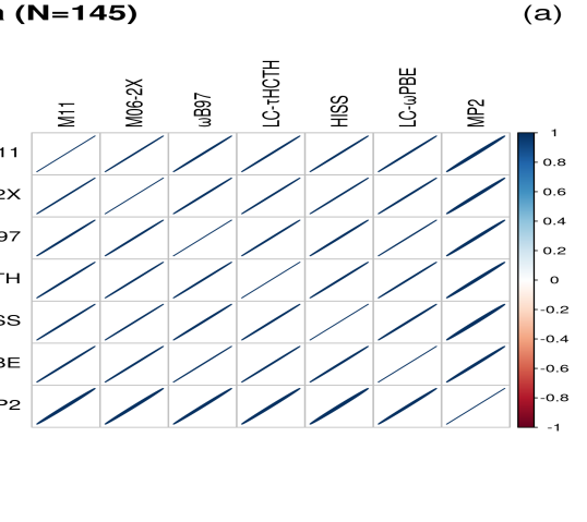
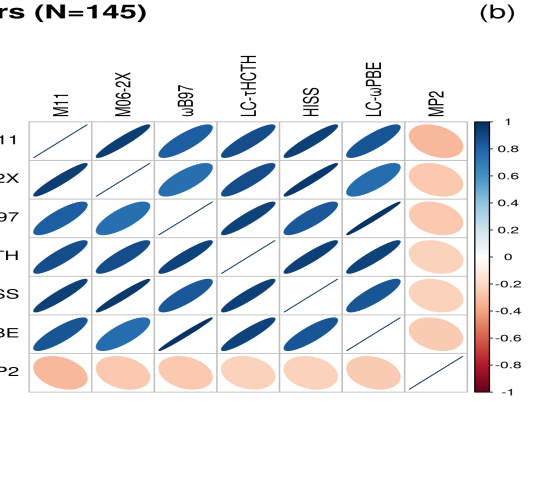
Figure 1: Rank correlation matrices between (a) data sets and (b) errors sets of polarizabilities for case WU2015 (Paper II (Pernot2020a, )).

For the example showcased in Fig. 1(a), one sees that all the datasets $C_{i}$ are all strongly positively correlated, meaning that all methods produce closely the same trend. By contrast, the error sets $E_{i}$ present a more relaxed pattern (Fig. 1(b)), with weaker positive correlations, and even a very small negative correlation for MP2 with all the other error sets. Having noticed this, one can remark that MP2 data present also smaller correlation coefficients with other datasets, although this is barely visible on the figure (the difference bears on the third digit of the correlation coefficients). In the following, we present correlation matrices for error sets only.

III Statistics, their uncertainty and correlation

III.0.1 Uncertainty

The value $s$ of a statistic $S$ (MSE, MUE, $Q_{95}$…) estimated on an error set is generally uncertain, with uncertainty estimated by its standard error $u(s)$. Two main uncertainty sources should be considered: (1) the limited size $N$ of the reference data sample, and (2) the uncertainty on errors, $u(e_{i})$ (Section II). Unless the dataset is exhaustive (e.g., a dataset containing a property for a complete class of systems), the first source is always present. For experimental reference data, the second source is also always present, but experimental uncertainty is rarely available for large datasets, and a common practice seems to be to ignore them in the statistical analysis (although they are often discussed to assess the quality of the dataset). Some studies considered the effect of representative uncertainty levels on benchmarking conclusions (Pernot2015, ; DeWaele2016, ; Proppe2017, ).

In Appendix A, the impact of both uncertainty sources is illustrated on the mean value (MSE), for which analytical formulae are available. The strategy to handle reference data uncertainty depends on their distribution. If the reference data uncertainties are uniform over the dataset, the hypothesis of i.i.d. errors holds, and standard statistical procedures can be applied (unless one is interested in quantifying specifically model errors (Pernot2015, ; Proppe2017, )). Otherwise, weighted statistics have to be used (Pernot2015, ; Proppe2017, ), which will not be considered here. Instead, we assume that datasets should not include data with extreme uncertainty values.

Simple formulae for standard errors, such as those for the mean (a linear statistic), are not available for non-linear statistics such as the MUE or $Q_{95}$. Moreover, in order to avoid some of the limitations implied by such formulae (e.g., normality hypothesis), one can use a general method to estimate the standard error of any statistic: the bootstrap (Efron1979, ; Efron1991, ; Hesterberg2015, ). It is a Monte Carlo sampling method which consists in random draws with replacement of $N^{\prime}$ values from a dataset of size $N$. In the standard bootstrap, one uses $N^{\prime}=N$, i.e., the generated samples have the same size as the original set. The bootstrap has been shown to provide reliable estimation of uncertainty, but the mean values unavoidably reflect the bias due to the original data set (Hesterberg2015, ). In consequence, we estimate in the following the mean values from the original sample and the uncertainties from the bootstrap samples. The main limitation of the bootstrap is its hypothesis of $i.i.d.$ data, but it is consistent with our choice to avoid reference datasets with a large uncertainty range.

III.0.2 Correlation

The statistics covariance $\mathrm{cov}(s_{1},s_{2})$ derives from the mathematical expression of $S$ and from the variances and covariance of the error sets, $\mathrm{cov}(E_{1},E_{2})$. To estimate $\mathrm{cov}(s_{1},s_{2})$ in the case of a linear statistic, one can directly apply the generalization of the combination of variances to several model outputs (GUM-Supp2, ). For the MSE, it is easy to demonstrate that the covariance is transferred in totality: $\mathrm{cov}(\overline{e}_{1},\overline{e}_{2})=\mathrm{cov}(E_{1},E_{2})$, where $\bar{x}$ is the mean value of $X$. More generally, for linear statistics, $\mathrm{cov}(E_{1},E_{2})=0\Longrightarrow\mathrm{cov}(s_{1},s_{2})=0$. For non-linear statistics, such as the MUE or $Q_{95}$, the combination of covariances is unsuitable, and Monte Carlo strategies are used.

To illustrate the transfer of correlation from error sets to non-linear statistics, we performed a Monte Carlo study, detailed in Appendix B, with scenarii implying diverse distribution shapes. A few trends can be derived from this study, notably that for the MUE and $Q_{95},$ $\mathrm{cor}(s_{1},s_{2})$ is a convex, positive function of $\mathrm{cor}(E_{1},E_{2})$. Moreover, for a given value of $\mathrm{cor}(E_{1},E_{2})$ one observes that $\mathrm{cor}(MUE_{1},MUE_{2})\geq\mathrm{cor}(Q_{95,1},Q_{95,2})$. As we explored only a fraction of the possible scenarii for the errors distributions, these trends should not be considered as general. Our main point is that the correlation of error sets is at least partially transferred to the derived statistics, a fact to be considered when comparing the values of these statistics.

IV Pair-wise comparison of errors

We define the systematic improvement probability (SIP) between two methods $M_{i}$ and $M_{j}$ as the proportion of systems in the reference set for which the absolute error decreases when using $M_{i}$ instead of $M_{j}$. It is estimated as

$$\mathrm{SIP}_{i,j} =\frac{D_{i,j}}{N}$$ (6)

$$D_{i,j} =\sum_{k=1}^{N}\mathbf{1}_{\Delta_{k}(M_{i},M_{j})<0}$$ (7)

where $\mathbf{1}_{X}$ is the indicator function, taking for value 1 if $X$ is true and 0 otherwise, and

$$\Delta_{k}(M_{i},M_{j})=|e_{k}(M_{i})|-|e_{k}(M_{j})|$$ (8)

Note that, because of the possible presence of ties, one has $\mathrm{SIP}_{i,j}+\mathrm{SIP}_{j,i}\apprle 1$.

IV.0.1 Interpretation

A row of the SIP matrix, provides the SIP values for the corresponding method over all the other ones. If a new method $M_{1}$ provides systematic improvement over $M_{2}$, in the sense that it has smaller absolute errors for all systems in the reference set, one should have $\mathrm{SIP}_{1,2}=1$. Values smaller than 0.5 indicate a degradation. Note however that $M_{1}$ can achieve small values of the SIP and still have better scores (MUE, $Q_{95}$), as a few large improvements might overwhelm many small degradations. The interest of the SIP indicator is mainly to alert the user that using a “better method” $M_{1}$ can lead to a degradation of results with respect to $M_{2}$, with a probability close to $(1-\mathrm{SIP}_{1,2})$.

IV.0.2 Mean SIP

In order to compare and rank a set of $K$ methods, one defines the Mean SIP (MSIP) as the mean value of a line of the SIP matrix (excluding the diagonal)

$$\mathrm{MSIP}(M_{i})=\frac{1}{K}\sum_{j=1}^{K}\mathrm{SIP}_{i,j}\,(1-\delta_{ij})$$ (9)

The largest MSIP value points to a method which in average provides the best level of improvement over the other methods in the set. Note that the MSIP is not transferable for comparisons with methods out of its definition set.

IV.0.3 Representation

In the same spirit as for correlation matrices, we represent SIP matrices by a combination of color levels and disks. Here, the color scale goes from blue (0.0) to red (1.0) with a white midpoint (0.5), and the area of the disks is proportional to the SIP value. The diagonal is null. The matrix should be read by row: a row with a majority of red patches signals a method with good SIP performances. A contrario, a majority of blue patches on a row indicate a method with poor SIP performances. The methods are ordered by decreasing value of MSIP.

Fig. 2 provides an example extracted from a benchmark for intensive atomization energies (case PER2018 in Paper II (Pernot2020a, )). It shows clearly that, for this dataset, BH&HLYP is problematic, with a row of small blue disks, and is systematically and strongly outperformed by all other methods. At the opposite, the row for CAM-B3LYP is the only one to contain exclusively values above 0.5 (reddish disks), albeit CAM-B3LYP does not achieve the best MUE nor $Q_{95}$ scores within this set of methods (Pernot2018, ; Pernot2020a, ). This conflict will be further discussed in Paper II (Pernot2020a, ).

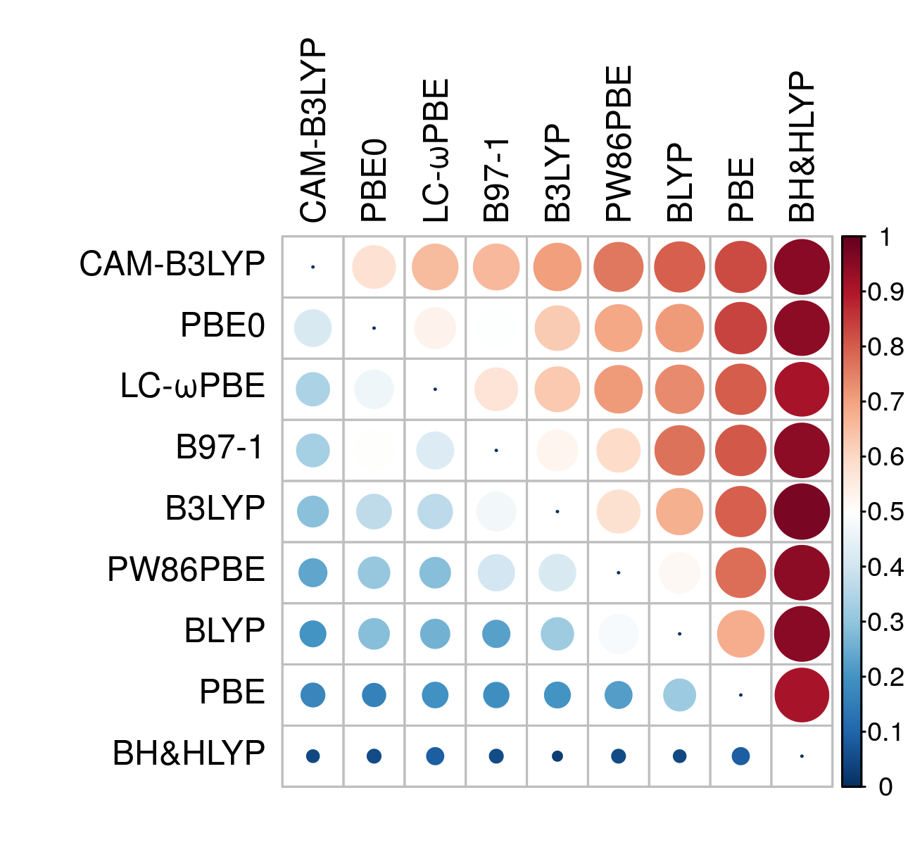
Figure 2: SIP matrix for a set of 9 methods compared on the G99 set of enthalpies (case PER2018, Paper II (Pernot2020a, )). The SIP value is color-coded and the area of a disk is proportional to the corresponding value. A row with a majority of red patches signals a method with good SIP performances. The methods are ordered by decreasing value of MSIP (Eq. 9).

IV.0.4 Mean gain and loss

In order to appreciate the amplitude of the possible losses or gains when switching between two methods, we define the mean gain (MG) as the mean of the negative values of $\Delta_{k}(M_{i},M_{j})$, which is only defined if $\mathrm{SIP}_{i,j}$ is non-null:

$$\mathrm{MG}_{i,j} =\frac{1}{D_{i,j}}\sum_{k=1}^{N}\mathbf{1}_{\Delta_{k}(M_{i},M_{j})<0}\,\Delta_{k}(M_{i},M_{j})$$ (10)

$$\mathrm{ML}_{i,j} =-\mathrm{MG}_{j,i}$$ (11)

where by construction the mean loss (ML) is equal the opposite of the mean gain for the reciprocal comparison.

These statistics are intended to convey an amplitude of the improvement of $M_{i}$ over $M_{j}$: MG is therefore a negative value (corresponding to a decrease of absolute errors), and ML a positive value. Moreover, the SIP, MG and ML provide a decomposition of the MUE difference between two methods:

$$\Delta_{\mathrm{MUE}_{i,j}} =\mathrm{MUE}(M_{i})-\mathrm{MUE}(M_{j})$$ (12)

$$=\mathrm{SIP}_{i,j}*\mathrm{MG}_{i,j}+\mathrm{SIP}_{j,i}*\mathrm{ML}_{i,j}$$ (13)

This shows that, except for method pairs with extreme SIP values, any MUE difference is the balance between losses and gains distributed over the systems. One should not expect that a method with a smaller MUE will systematically provide better results.

IV.0.5 ECDF of $\Delta_{k}(M_{i},M_{j})$

The scores (SIP, MG and ML) can be visualized on a single graph of the Empirical Cumulated Density Function (ECDF) of the differences of absolute errors between two methods, as shown in Fig. 3(b). This example is extracted from the benchmark dataset BOR2019 presented in Paper II (Pernot2020a, ), on the prediction of band gaps. It compares mBJ (MUE = 0.50 eV) and LDA (MUE = 1.17 eV). Each point of the ECDF corresponds to a system of the dataset. Systems with negative differences are those for which mBJ performs better than LDA.

The large MUE difference ($\Delta_{\mathrm{MUE}}$) between these methods is the balance of a mean gain $\mathrm{MG}=-0.86$ eV for 85 % of the systems (SIP), and a mean loss $\mathrm{ML}=0.37$ eV for 15 % of the systems. In the hypothesis of a representative dataset, a user switching from LDA to mBJ has to accept a 15 % risk to see his LDA results degraded in average by 0.37 eV, and up to 1 eV.

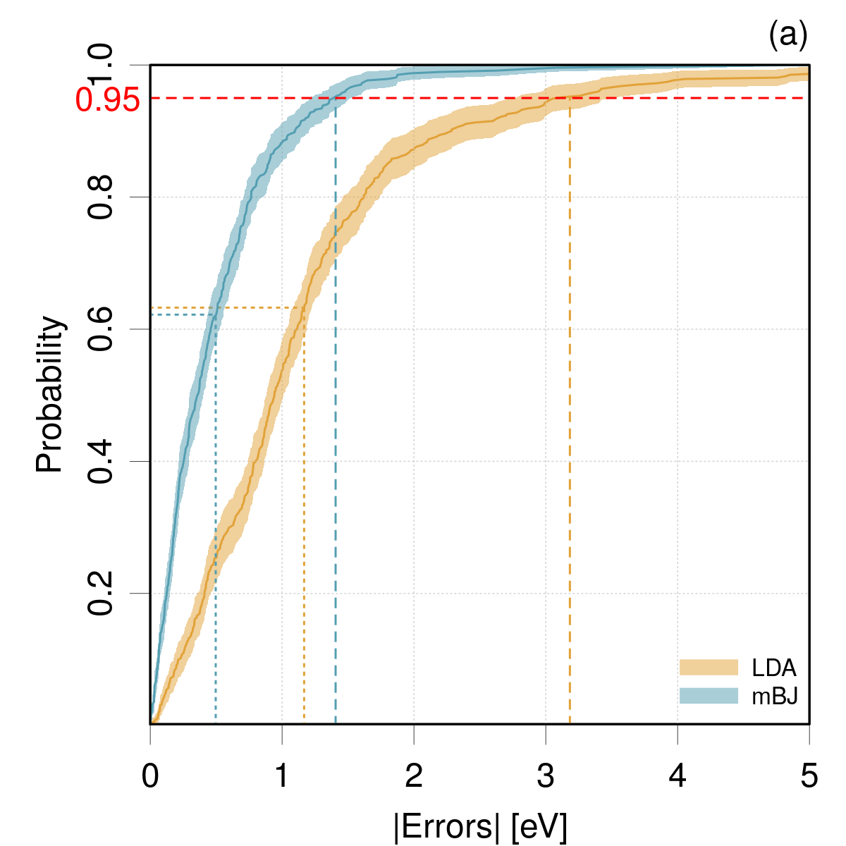
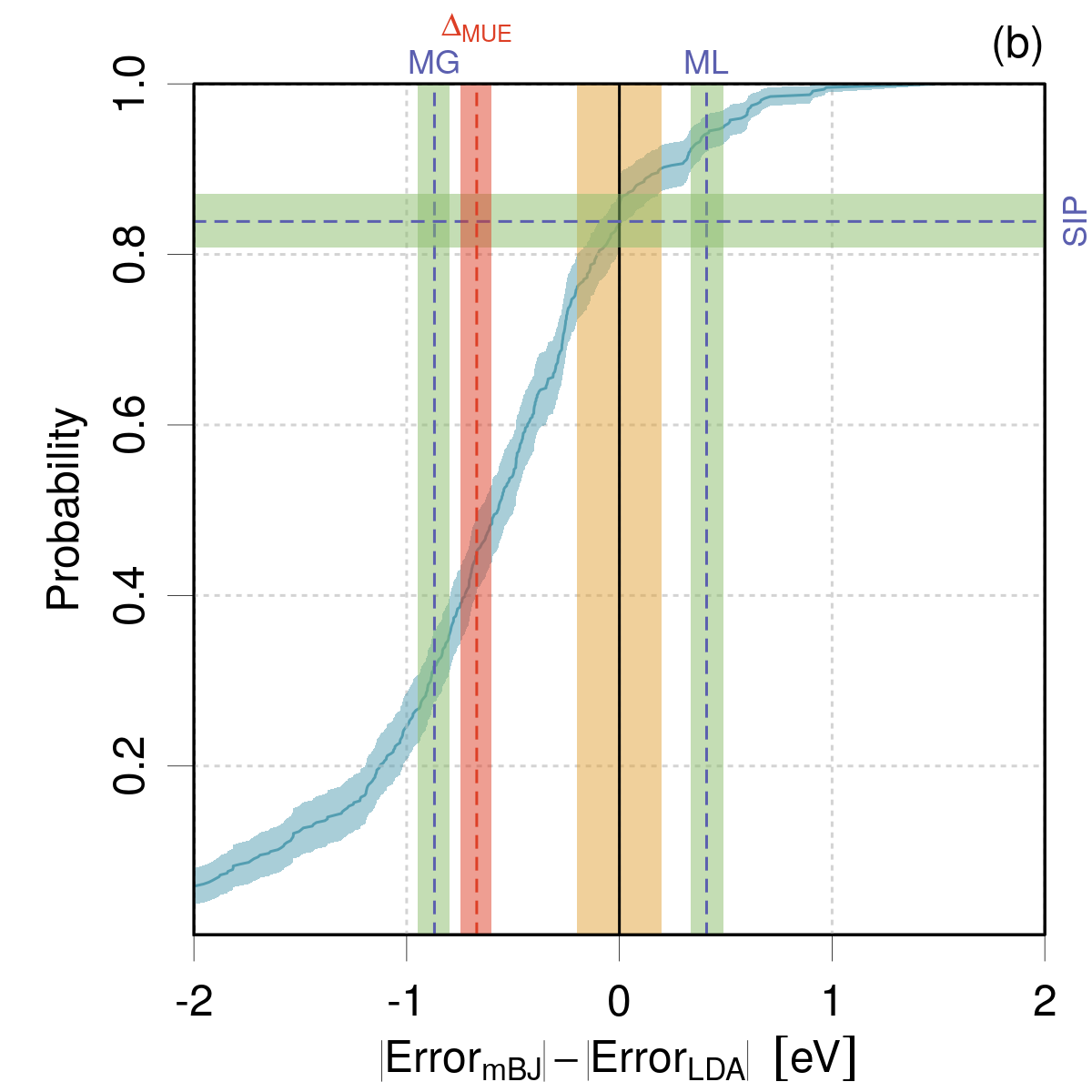
Figure 3: Statistics of absolute errors on band gaps for methods mBJ and LDA (case BOR2019, Paper II (Pernot2020a, )) and of their pair-wise differences: (a) ECDF of two error sets to be compared. The MUE values are depicted by vertical dotted lines, and the $Q_{95}$ values by vertical dashed lines. The confidence bands cover 95% probability; (b) ECDF of the difference of absolute errors (blue curve and confidence band). The green- and red-shaded bands represent 95 % confidence intervals for the reported statistics (SIP: systematic improvement probability; MG: mean gain; ML: mean loss, $\Delta_{MUE}$: MUE difference). The orange vertical bar represents an estimated level of uncertainty in the dataset. It is a visual aid to evaluate the pertinence of the observed differences.

Note that this information is not accessible when considering the ECDFs of the absolute errors (Fig. 3(a)). For the chosen example, the comparison of these ECDFs might leave the false impression that mBJ has consistently smaller absolute errors than LDA, which is an artifact due to the missing information about data pairing (correlation) in this representation.

V Pair-wise comparison of statistics

V.1 The testing framework

Using the error sets for two methods $M_{1}$ and $M_{2}$, one calculates the values $s_{1}=S(E_{1})$ and $s_{2}=S(E_{2})$ of a statistic $S$. A common procedure to compare two values is to test if their difference is significantly larger than their combined uncertainty, i.e.

$$|s_{1}-s_{2}|>\kappa\thinspace u(s_{1}-s_{2})$$ (14)

where $u(s_{1}-s_{2})$ is the uncertainty on the difference, and $\kappa$ is an enlargement factor typically taken as $\kappa=2$ (or 1.96) in metrology (Kacker2010, ). In the hypothesis of a normal distribution for the statistics difference, $\kappa=1.96$ corresponds to a confidence level of 95 % for a two-sided test, implied by the absolute value in Eq. 14. If one has evidence that the distribution of differences is not normal, $\kappa$ has to be chosen as the uncertainty enlargement factor providing a 95 % confidence interval for this distribution. If the test is positive, there is less than 5 % probability that the difference between $s_{1}$ and $s_{2}$ is due to sampling effects.

Assuming that $u(s_{1}-s_{2})$ cannot be null nor infinite, it is convenient to recast the test by using a discrepancy factor

$$\xi(s_{1},s_{2})=\frac{|s_{1}-s_{2}|}{u(s_{1}-s_{2})}$$ (15)

to be compared to the threshold $\kappa$. A probability value ($p$-value) corresponding to $\xi$ is derived from the cumulated density function of the expected distribution for $\xi$. For instance

$$p_{t} =1-\Phi_{H}(\xi)$$ (16)

$$=2*\left(1-\Phi(\xi)\right)$$ (17)

where $\Phi_{H}(.)$ is the cumulative distribution function (CDF) of the standard half-normal distribution (Leone1961, ), and $\Phi(.)$ is the CDF of the standard normal distribution. The half-normal distribution is used to account for the absolute value in Eq. 15. The $t$ index of $p_{t}$ refers here to the analogy with the two-sample $t$-test for equal means (Snedecor1989, ). $p_{t}$ is the probability to obtain values of $\xi$ equal to or larger than the calculated value, assuming that the null hypothesis, $S(E_{1})=S(E_{2})$, is true. For testing, one chooses a probability threshold corresponding to $P(\xi>\kappa=1.96)=0.05$ . For $p_{t}$ above this value, one chooses not to reject the hypothesis that the observed difference between $s_{1}$ and $s_{2}$ is due to random effects.

In order to be able to estimate $p_{t}$, one needs to evaluate the uncertainty on the difference of $s_{1}$ and $s_{2}$. Formally, it can be obtained by the combination of variances (GUM, )

$$u(s_{1}-s_{2})=\sqrt{u^{2}(s_{1})+u^{2}(s_{2})-2\mathrm{cov}(s_{1},s_{2})}$$ (18)

The usefulness of this formula depends on several assumptions (theoretical limits of the statistics not within a high probability interval around their values, symmetry of error intervals… (Nicholls2014, ; Nicholls2016, )). Nevertheless, it shows that the covariance between statistics can have a major effect on the amplitude of $u(s_{1}-s_{2})$. In the limit of very strong positive correlation, the uncertainty on the difference can become very small, impacting $\xi(s_{1},s_{2})$ and $p_{t}$.

To estimate the effect of correlation on the comparison of scores, we introduce a variant $p_{unc}$ (uncorrelated) of $p_{t}$, based on a version of the discrepancy ignoring correlation

$$\xi_{unc}(s_{1},s_{2}) =\frac{|s_{1}-s_{2}|}{\sqrt{u(s_{1})^{2}+u(s_{2})^{2}}}$$ (19)

$$p_{unc} =2*\left(1-\Phi(\xi_{unc})\right)$$ (20)

In the hypothesis of mostly positive correlations for the statistics of interest (MUE and $Q_{95}$; Appendix B), $p_{unc}$ is expected to overestimate $p_{t}$.

V.2 Bootstrap-based comparison of statistics

Several strategies can be considered to compare pairs of statistics $(s_{1},s_{2})$ through a $p$-value.

V.2.1 Estimate $u(s_{1})$, $u(s_{2})$ and $\mathrm{cov}(s_{1},s_{2})$

The uncertainty on the statistics of interest (except for the MSE and RMSD) and their covariance are not, to our knowledge, available in analytical form. In consequence, one has to use a numerical procedure, such as the bootstrap to estimate them (Efron1979, ; Hesterberg2015, ). The application of the bootstrap to individual terms of Eq. 18 will result in an accumulation of statistical uncertainties. Besides, the estimation of covariances is known to be very sensitive to outliers. This approach is clearly suboptimal and is not recommended.

V.2.2 Estimate directly $u(s_{1}-s_{2})$

A better approach in the present context is to estimate directly (by bootstrap) the uncertainty on the difference of scores. This relieves underlying hypotheses in Eq. 18, and enables the explicit correlation of samples of $s_{1}$ and $s_{2}$ through paired-data sampling. However, estimating a discrepancy factor leads us to use Eq.17 to estimate the $p$-value, with the associated normality hypothesis.

V.2.3 Generalized $p$-value

The use of the generalized $p$-value ($p_{g}$), as proposed by Wilcox and Erceg-Hurn (Liu1997, ; Wilcox2012, ) (method M; cf. Algorithm 1), conveniently avoids to estimate $u(s_{1}-s_{2})$, and the incurring normality hypothesis of $p_{t}$. It is based on a simple counting of null and negative bootstrapped differences of statistics with paired samples. If $S(E_{1})=S(E_{2})$, one expects that the bootstrap sample will generate positive and negative values of their difference in equal amounts. In this case, $p^{*}\simeq 1-p^{*}\simeq 0.5$ and $p_{g}$ is close to 1. Note that the null values in the differences sample are shared equally between the positive and negative values. On the opposite, if there is a small proportion $p^{*}$ of negative values, the mean of the differences sample should be positive, different from zero. The smaller $p^{*}$ the farther the mean from zero, and the lower the probability of the null, $S(E_{1})=S(E_{2})$, hypothesis. The symmetric case occurs for large values of $p^{*}$ (small values of $1-p^{*}$). As the sign of the difference is irrelevant, a factor two is applied to estimate $p_{g}$. The identity of this algorithm with the analytical $p$-value for the comparison of the means of normal samples is established in Appendix D.2.

Input: Two paired error sets $E_{1}$, $E_{2}$ of size $N$, a statistic estimator $S$, and a number of bootstrap samples $B$

1. Bootstrap the statistics difference

   1. For $j=1:B$

      1. Generate a $N$-sample of paired data with replacement $\longrightarrow\left(E_{1}^{*},E_{2}^{*}\right)$

      2. Estimate $d_{j}=S(E_{1}^{*})-S(E_{2}^{*})$

2. Calculate a generalized $p$-value to test $S(E_{1})=S(E_{2})$

   $p_{g}=2\min(p^{*},1-p^{*})$, where
   $p^{*}=(A+0.5C)/B$
   $A=\sum_{i=1}^{B}1_{d_{i}<0}$
   $C=\sum_{i=1}^{B}1_{d_{i}=0}$

Algorithm 1 Method M: testing the equality of a statistic $S$ for two paired samples by bootstrap and a generalized $p$-value ($p_{g}$) (Wilcox2012, ).

The use of paired samples is essential to capture inter-statistics correlations. Wilcox and Erceg-Hurn (Wilcox2012, ) have shown that their method M provides a well controlled level of type I errors (false positive) for the comparison of quantiles at the 0.05 level. They estimated that dataset sizes of $N\geq 30$ are necessary when comparing quantiles up to 0.9. This applies to the MUE, which we have shown to lie typically between the 0.5 and 0.75 quantiles (Pernot2018, ). Using the same protocol, we estimated that for the comparison of $Q_{95}$ values at the same 0.05 level, $N\geq 60$ is requested. Details are presented in Appendix C.

V.3 Rank inversion probability $P_{inv}$

In a previous article (Pernot2018, ), we defined a ranking inversion probability

$$P_{inv}=P(S_{1}<S_{2}|s_{1}>s_{2})$$ (21)

and estimated it using the hypothesis of a normal distribution for the difference of statistics. Using Equations 19-20, this former estimation can be reformulated as

$$P_{inv} =\Phi(0;\mu=s_{1}-s_{2},\sigma=\sqrt{u^{2}(s_{1})+u^{2}(s_{2})})$$ (22)

$$=\Phi(0;\mu=\xi_{unc})$$ (23)

$$=\Phi(-\xi_{unc})$$ (24)

$$=1-\Phi(\xi_{unc})$$ (25)

$$=p_{unc}\thinspace/\thinspace 2$$ (26)

where the unspecified parameters of the normal cumulative distribution function $\Phi(x;\mu,\sigma)$ are their standard values ($\mu=0$, $\sigma=1$). The link to $p_{unc}$ shows the limitations of our previous estimation of $P_{inv}$, i.e., the normality hypothesis and the neglect of error sets correlations.

Using the same difference statistics used for $p_{g}$ (Algorithm 1), one can generalize Eq. 21 by defining $P_{inv}$ as the probability to have differences in the bootstrap sample with a sign opposite to the reference one ($\mathrm{sign}(s_{1}-s_{2})$)

$$P_{inv} =\frac{1}{B}\left(\sum_{i=1}^{B}1_{\mathrm{sign}(d_{i})\neq\mathrm{sign}(s_{1}-s_{2})}-\sum_{i=1}^{B}1_{d_{i}=0}\right)$$ (27)

where $B$ is the number of bootstrap samples and the null differences (with sign 0) are compensated for. Enforcing the condition $s_{1}>s_{2}$ in Eq. 21, one gets $\mathrm{sign}(s_{1}-s_{2})=1$, and finally

$$P_{inv} =\frac{1}{B}\left(\sum_{i=1}^{B}1_{\mathrm{sign}(d_{i})\neq 1}-\sum_{i=1}^{B}1_{d_{i}=0}\right)$$ (28)

$$=\frac{1}{B}\left(\sum_{i=1}^{B}1_{d_{i}\leq 0}-\sum_{i=1}^{B}1_{d_{i}=0}\right)$$ (29)

$$=\frac{1}{B}\sum_{i=1}^{B}1_{d_{i}<0}$$ (30)

$$\simeq p_{g}\thinspace/\thinspace 2$$ (31)

where the relation to $p_{g}$ (Algorithm 1) assumes a negligible probability to have null statistics differences and exploits the fact that $\sum_{i=1}^{B}1_{d_{i}<0}<\sum_{i=1}^{B}1_{d_{i}>0}$ if $s_{1}>s_{2}$.

V.4 Ranking probability matrix $\mathbf{P}_{r}$

A measure of the reliability of a statistic-based ranking can be estimated by bootstrap (Hall2009, ). This approach has notably been used by Proppe and Reiher (Proppe2017, ) to study how the sample size affects the probability for a DFA to be ranked at first place on the basis of its prediction uncertainty. We apply it here to compute, for a set of $K$ methods scored by a statistic $S$, a ranking probability matrix $\mathbf{P}_{r}$ giving, for each method, its probability to have any rank

$$P_{r,jk}=P(\mathrm{rank}(S_{j})=k);\thinspace j,k=1,\ldots,K$$ (32)

The algorithm to generate this matrix is described in Algorithm 2.

Input: $K$ paired error sets, $E_{1},\ldots,E_{K}$ of size $N$, a statistic estimator $S$, and a number of bootstrap samples $B$

1. Bootstrap the ranks

   1. For $j=1:B$

      1. Generate a $N$-sample of paired data with replacement $\longrightarrow\left(E_{1}^{*},\ldots,E_{K}^{*}\right)$

      2. Estimate the statistics vector $S^{*}=\left(S(E_{1}^{*}),\ldots,S(E_{K}^{*})\right)$

      3. Estimate the ranks by increasing order of $S^{*}$: $O_{j}^{*}=\mathrm{order}(S^{*})$,
         where $O_{j}^{*}$ is a $K$-vector of integer values.

2. Estimate for each method its probability to have any rank

   $$P_{r,jk}=\frac{1}{B}\sum_{i=1}^{B}1_{O_{ij}^{*}=k}$$

Algorithm 2 Estimating the rank probabilities for a set of methods.

V.4.1 Representations

Two representations for this matrix are proposed by Hall and Miller (Hall2009, ), either a combined color-levels / symbol-size image (Fig. 4(a)), or a summary by mode and probability intervals (Fig. 4(b)). In the following, we will use mostly the levels image representation which we find easier to read and interpret.

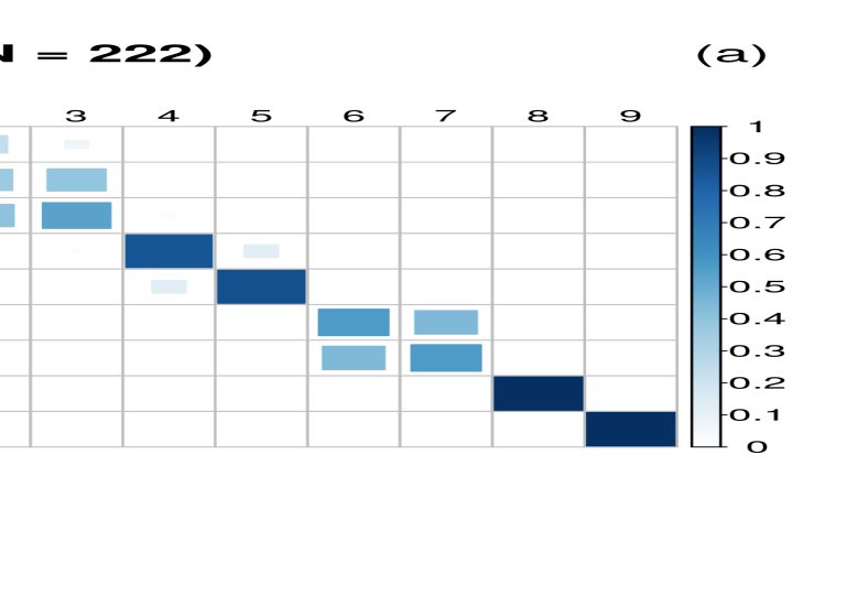
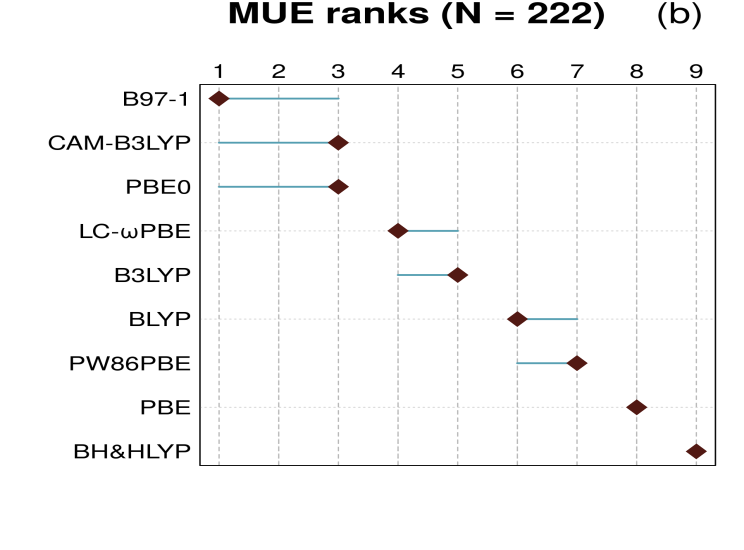
Figure 4: Graphical representations of a MUE ranking probability matrix $\mathbf{P}_{r}$ : (left) color levels image of the ranking probability matrix; (right) summary of the ranking probability matrix by the modes (diamonds) and 90 % probability intervals. The data are taken from the case PER2018 (cf. Paper II (Pernot2020a, )). Both representations indicate a possible ranking inversion between B97-1, CAM-B3LYP and PBE0, i.e., the reference ranking based on the MUE is not certain for this trio. Similar problems occur within two other groups, notably BLYP and PW86PBE. The ranks of PBE (8) and BH&HLYP (9) are well established.

V.4.2 Remarks

• As discussed by Hall and Miller (Hall2009, ), the standard bootstrap ($N$-out of-$N$ sampling) tends to underestimate the dispersion of the ranks. Better estimates would be obtained by a $N^{\prime}$-out of-$N$ sampling ($N^{\prime}<N$), but the best choice of $N^{\prime}$ is problem-dependent and is left to the appreciation of the analyst. For the sake of simplicity, and until further guidance on the optimal choice of $N^{\prime}$, we consider here that the standard method provides a reasonable qualitative appreciation of ranking uncertainties. An example with $N^{\prime}=N/3$ is presented in case DAS2019 of Paper II (Pernot2020a, ).

• As a general trend, one expects that ranking uncertainty will increase for smaller error sets, but might also increase with the number $K$ of compared methods, notably if several methods have similar performances.

VI Implementation

Calculations have been made in the R language (CiteR, ), using several packages, notably for the bootstrap (boot (R-boot, )). Bootstrap estimates are based on 1000 replicates.

Quantiles.

Wilcox and Erceg-Hurn (Wilcox2012, ) recommend the use of the Harrell and Davis method for quantiles estimation (Harrell1982, ), which provides a better stability for the bootstrap sampling of quantiles. The relevance of this choice is illustrated in Appendix D. In the case studies of Paper II (Pernot2020a, ), all quantiles are estimated by the Harrell and Davis method (Harrell1982, ), as implemented in package WSR2 (Wilcox2012, ; Wilcox2018, ; R-WRS2, ).

Correlation.

The estimation of correlation coefficients by the standard Pearson method is reputed to be very sensitive to the presence of outliers (Wilcox2018, ). As the presence of a small amount of outliers is a frequent feature of the benchmarking data sets, we use the more robust rank-correlation (Spearman) method, unless otherwise specified.

Code.

The application ErrView implementing the methods described in this article (and more) and the corresponding datasets are archived at https://github.com/ppernot/ErrView (DOI: 10.5281/zenodo.3628489); a test web interface is also freely accessible at http://upsa.shinyapps.io/ErrView.

VII Conclusions

In this article, we proposed several tools to test the robustness of rankings or comparisons of methods based on error statistics for non-exhaustive, limited size datasets. In order to avoid hypotheses on the errors distributions, bootstrap-based methods were adopted, as suggested by Proppe and Reiher (Proppe2017, ) for the estimation of prediction uncertainty of DFT methods. Special care has been taken to use (robust) methods best adapted to provide reliable results for small datasets.

We introduced the systematic improvement probability (SIP) which is independent of other descriptive statistics. We have shown that the use of MUE for ranking hides a complex interplay between genuine method improvements and error cancellations inherent to most computational chemistry methods. In particular, we have shown how a difference in MUE is a balance between gains and losses in absolute errors. Estimation of the systematic improvement probability (SIP), the mean gain (MG) and mean loss (ML) statistics can help understand this balance, and to assess the risks for a user of switching between two methods.

When considering pairs of methods, we generalized our previous definition of the inversion probability $P_{inv}$ to account for correlations between statistics and relieve a normal distribution hypothesis. The link of $P_{inv}$ to $p$-values for the comparison of two values of a statistic has been established.

Finally, the ranking probability matrix $\mathbf{P}_{r}$ for a chosen statistic provides a clear diagnostic on the robustness of the corresponding ranking.

All these tools are put to test in Paper II (Pernot2020a, ),on nine datasets from the recent benchmark literature.

Supplementary Information

The data that support the findings of this study are openly available in Zenodo at
http://doi.org/10.5281/zenodo.3678481(SIPdata2020, ).

Appendix A Estimation of the mean value and its uncertainty

Let us consider the mean (signed) value of the errors (MSE). In absence of uncertainty, it is defined as

$$\overline{e}=\frac{1}{N}\sum_{i=1}^{N}e_{i}$$ (33)

and its uncertainty (standard error) is estimated as

$$u(\overline{e})=\sqrt{\frac{s_{e}^{2}}{N}}$$ (34)

where $s_{e}^{2}$ is a sample-based estimator of the population variance

$$s_{e}^{2}=\frac{1}{N-1}\sum_{i=1}^{N}(e_{i}-\overline{e})^{2}$$ (35)

Eq. 34 gives the well-known dependence of the MSE uncertainty with the dataset size for independent and identically distributed (i.i.d.) errors, assuming a finite variance, which might exclude error sets with heavy-tailed distributions, e.g., Cauchy.

If uncertainty on errors $u(e_{i})$ is negligible, $s_{e}$ is an estimation of the standard deviation of the errors distribution $\sigma$, which represents the dispersion of model errors. If the reference data are uncertain, $s_{e}$ quantifies a dispersion due to both model errors and reference data uncertainty. In consequence, it overestimates the dispersion of model errors, and specific models have to be designed if one wishes to estimate this specific contribution (Pernot2015, ; Proppe2017, ). This points to the necessity of using accurate reference data if the benchmark based on standard statistics is to reflect the properties of the studied methods.

To be more specific, in the presence of uncertainty on errors, the weighted mean is the maximum likelihood estimator of the distribution mean under normality assumptions (Bevington1992, )

$$\overline{e} =\sum_{i=1}^{N}w_{i}e_{i}$$ (36)

$$w_{i} =\frac{u(e_{i})^{-2}}{\sum_{j=1}^{N}u(e_{j})^{-2}}$$ (37)

giving less weight to the more uncertain data. Direct application of the combination of variances to this expression leads to (Bevington1992, )

$$u(\overline{e})^{2}=\frac{1}{\sum_{j=1}^{N}u(e_{j})^{-2}}$$ (38)

Note that in the case of identical uncertainty for all data, one recovers the expression for the unweighted case (Eq. 34).

The validity of this estimation has to be tested by computing the weighted chi-squared

$$\chi_{w}^{2}=\sum_{i}\frac{(e_{i}-\overline{e})^{2}}{u(e_{i})^{2}}$$ (39)

If the errors on the reference data are assumed to be normally distributed, $\chi_{w}^{2}$ has a chi-squared distribution with $N-1$ degrees of freedom ($\chi_{N-1}^{2}$). $\chi_{w}^{2}$ should be close to the mean of this distribution, $N-1$, and lie within its 95 % high probability interval. If $\chi_{w}^{2}$ is too small, the $u(e_{i})$ are over-estimated and should be reconsidered, or the benchmarked method is over-fitting the data, which is unlikely, unless the method is parametric and has been calibrated on this same dataset. If $\chi_{w}^{2}$ is too large, there is an excess of variance in the $E_{M}$ error set (Kacker2004, ; Rukhin2009, ; Rivier2014, ). In the typical benchmarking of computational chemistry methods, this is generally the case because of the extraneous dispersion due to model errors. To ensure the statistical validity of the weighted mean and its uncertainty, one has therefore to define a more complex error model, considering explicitly the two sources of dispersion, and to redefine the weights, accounting for the excess of variance and possible biases in the error sets (Lejaeghere2014, ; Lejaeghere2014a, ; Pernot2015, ; DeWaele2016, ; Proppe2017, ).

If one stipulates that the dispersion of the errors is the combined effect of model error and reference data uncertainty, one can redefine the weights as (Rukhin2009, )

$$w_{i}=\frac{\left(\sigma^{2}+u(e_{i})^{2}\right)^{-1}}{\sum_{j=1}^{N}\left(\sigma^{2}+u(e_{j})^{2}\right)^{-1}}$$ (40)

where $\sigma^{2}$ is the variance of model errors. With these new weights,

$$u(\overline{e})^{2}=\frac{1}{\sum_{j=1}^{N}\left(\sigma^{2}+u(e_{j})^{2}\right)^{-1}}$$ (41)

converges properly to the standard limit when the reference data errors become negligible before the model errors. The model error variance $\sigma^{2}$ can be estimated by decomposing the total variance of the errors into the variance of model errors plus the mean variance of the data (known as Cochran’s ANOVA estimate (Kacker2004, ; Rivier2014, ))

$$\mathrm{var}(e)=\sigma^{2}+\frac{1}{N}\sum_{j=1}^{N}u(e_{j})^{2}$$ (42)

This variance analysis ensures that $\chi_{w}^{2}$ is correct. Note that other reweighting schemes exist (Kacker2004, ; Rivier2014, ), but Cochran’s is the simplest. Besides, reweighting methods are iterative: $\sigma$ depends on $\overline{e}$, which itself depends on $\sigma$.

If the dispersion of reference data uncertainties is small, i.e., smaller than the model errors contribution, one can reasonably consider that the weights are identical and that the unweighted mean can be used. Formally, its uncertainty (Eq. 41) depends on $\sigma$, which can be directly estimated through Eq. 42, but by construction, one will recover results given by Eq. 34.

One will therefore consider that, unless a large dispersion of reference data uncertainty is observed, these uncertainties can be ignored in the estimation of the mean and its standard error. Otherwise, one should use the weighted mean with the standard uncertainty estimate.

An advanced modeling of uncertainty sources is crucial if one wishes a reliable estimate of the MSE, and of the various uncertainty contributions (Pernot2015, ). In standard benchmarking, the aim is mostly to compare methods, knowing that the reference datasets are incomplete. If reference data uncertainty plays a significant role – that would be the case if data with very different uncertainty levels were aggregated in the dataset – one might assume that its impact will be the same for all methods to be compared. The values of the dispersion statistics will be consistently overestimated for all methods. As long as one is not interested in the accurate estimation of the underlying properties of the error distributions, such as the model prediction uncertainty (Pernot2015, ; Proppe2017, ), it is simpler to rely on unweighted schemes and properly curated datasets.

Appendix B Numerical study of the correlation of nonlinear statistics

To illustrate the transfer of correlation from errors sets $E_{1}$ and $E_{2}$ to their statistics, one assumes that they are described by a bivariate distribution with prescribed correlation coefficient $\rho$. From this distribution, one generates random samples $E_{1}^{*}$ and $E_{2}^{*}$ and one estimates the statistics values $s_{1}^{*}=S(E_{1}^{*})$ and $s_{2}^{*}=S(E_{2}^{*})$. $\mathrm{cor}(s_{1},s_{2})$ is finally estimated from $s_{1}^{*}$ and $s_{2}^{*}$ samples.

The error sets correlation coefficient $\rho$ is varied between -1 and 1, and the resulting correlation coefficients are estimated for the MSE, MUE and $Q_{95}$ statistics. The dataset size is $N=100$ and Monte Carlo samples size is $M=10^{3}$ .

The results for four representative cases of the g-and-h distribution used by Wilcox and Erceg-Hurn (Wilcox2012, ) (Appendix E) of error sets are reported in Fig. 5(a-d). In this example, both error sets $E_{1}$ and $E_{2}$ have the same distribution with unit variance, only their correlation varies.

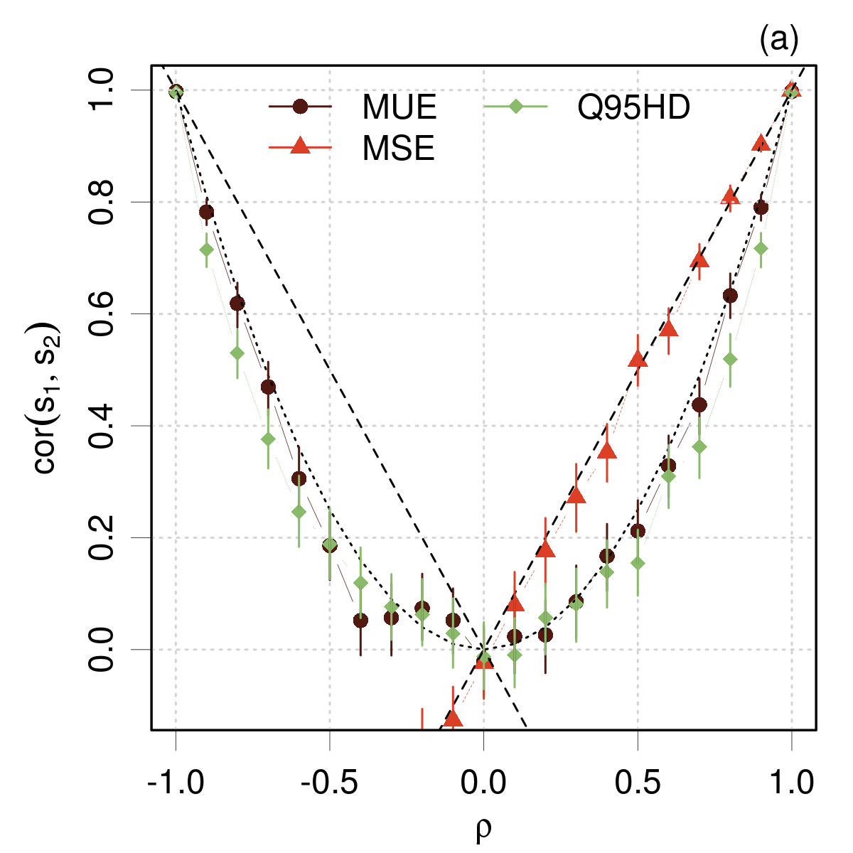
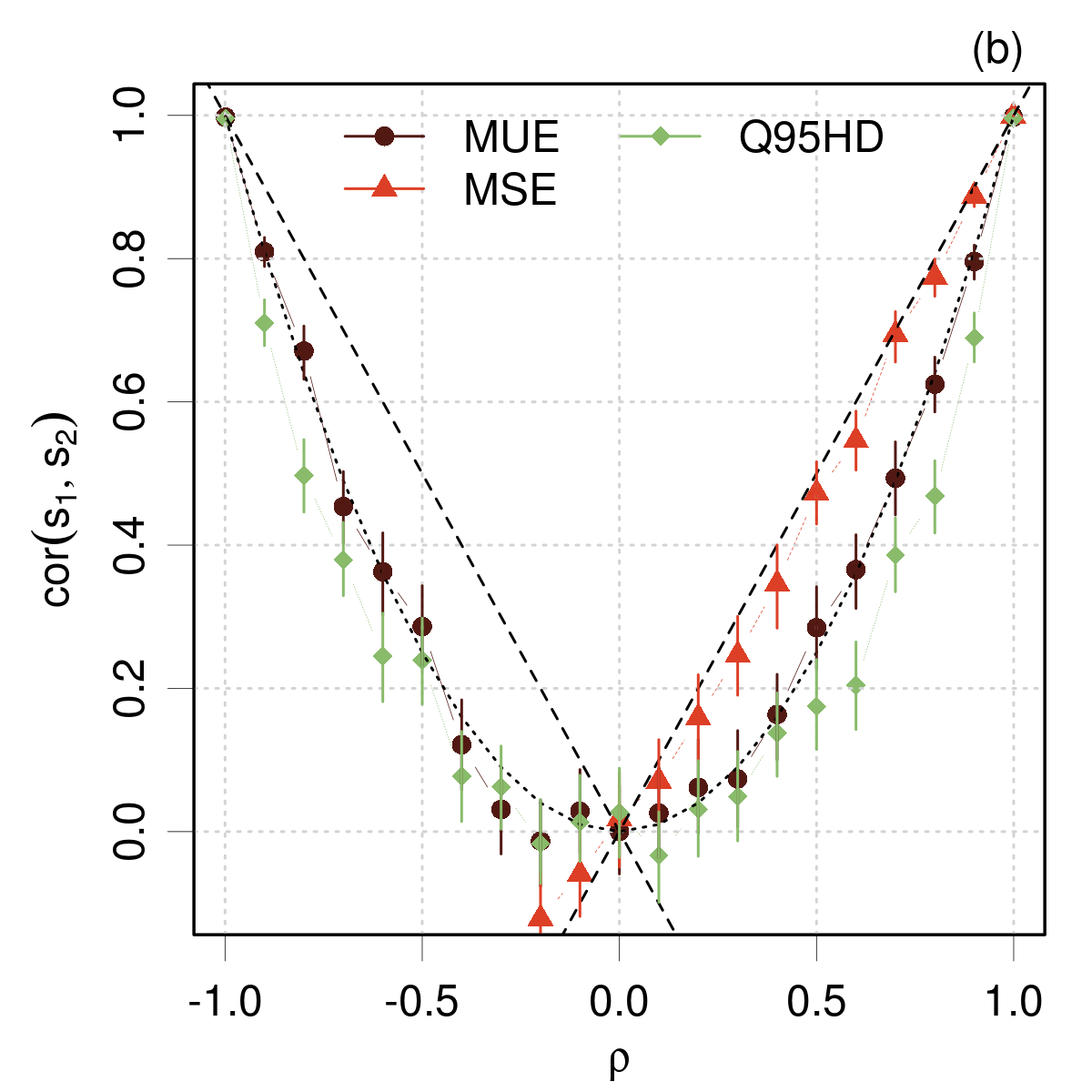
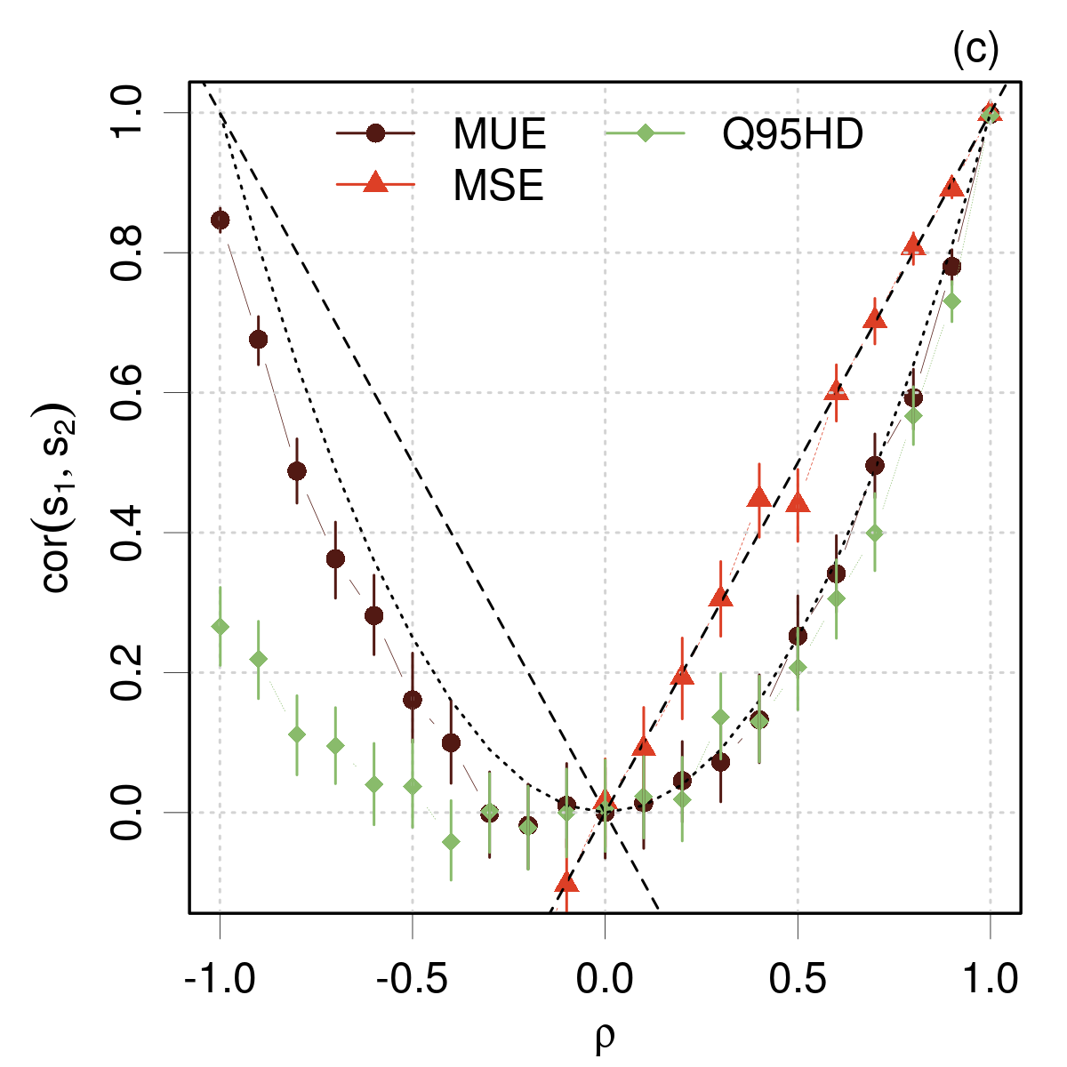
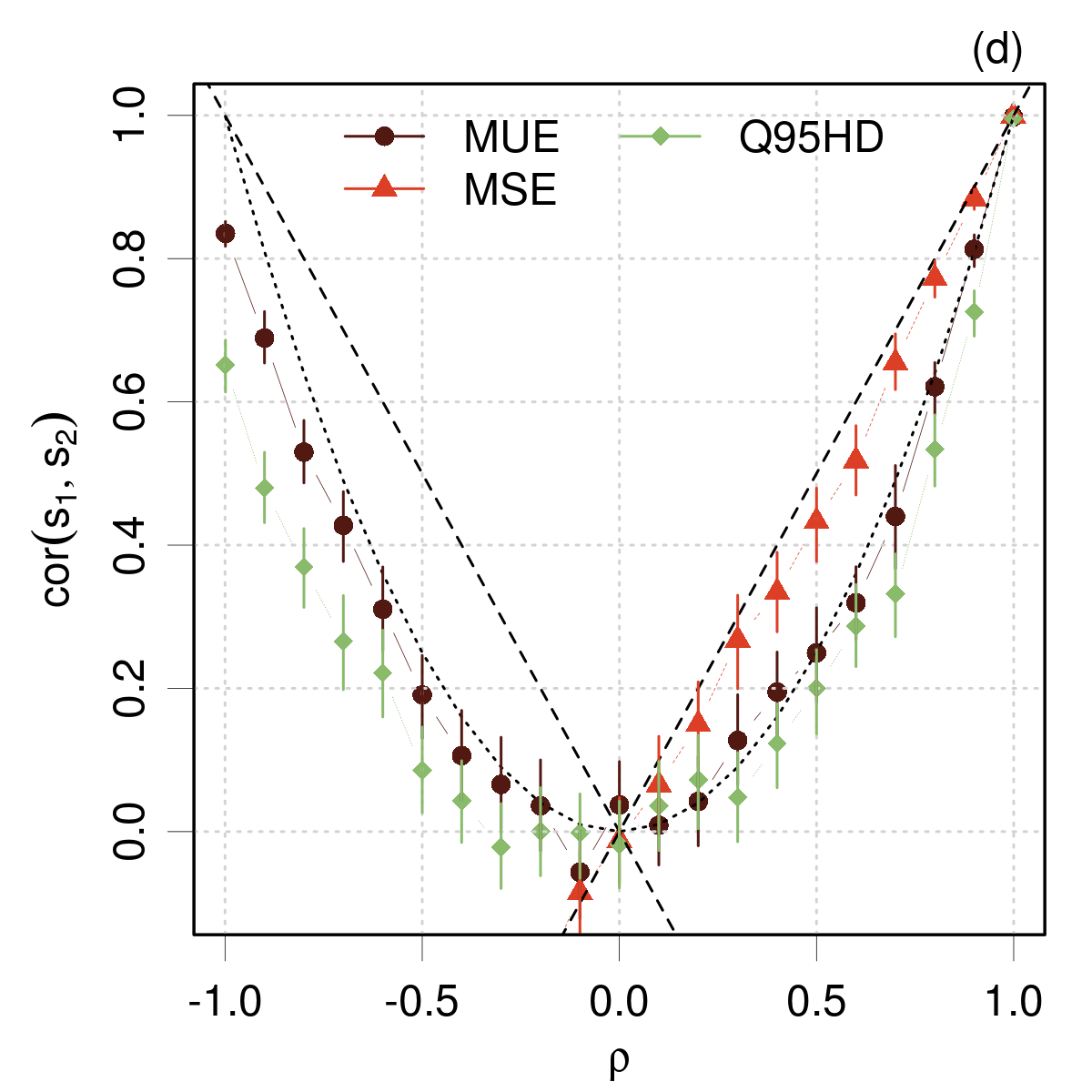
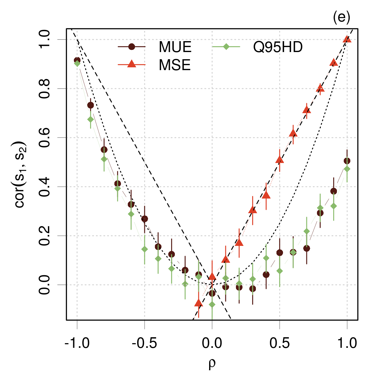
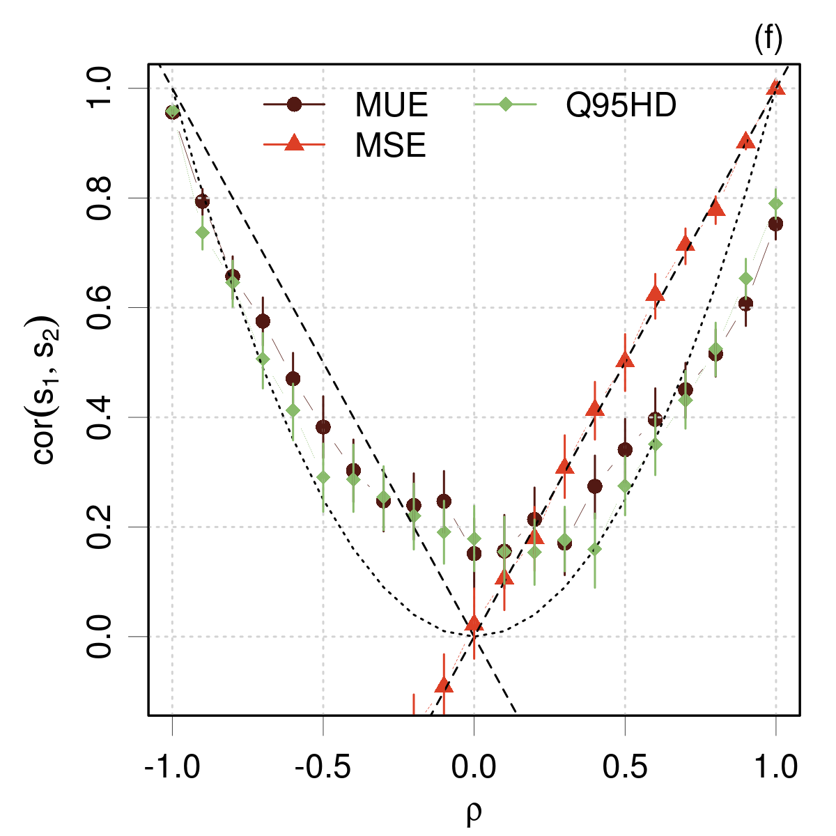
Figure 5: Correlation coefficients $\mathrm{cor}(s_{1},s_{2})$ of statistics ($S=$ MUE, MSE, $Q_{95})$ for two samples as a function of the correlation coefficient $\rho$ of these samples. The error bars represent 95 % intervals for sampling errors. Four cases of the g-and-h distribution are considered for the error sets: (a) normal ($g=h=0$); (b) heavy-tailed symmetric ($g=0;\thinspace h=0.2$); (c) light-tailed asymmetric ($g=0.2;\thinspace h=0$); (d) heavy-tailed asymmetric ($g=h=0.2$). Additional cases with shifted distributions, $\mu$= (-0.2,0.5) : (e) Normal ; (f) Student’s-$t$ ($\nu$= 5). All distributions have unit variance.

These simulations confirm the full correlation transfer to the MSE, independently of the underlying distribution. The correlation coefficients for the other, non-linear, statistics are mostly positive (within numerical uncertainty) and systematically smaller than $|\rho|$. They are symmetrical with respect to $\rho=0$ for symmetrical error distributions. The values for the MUE are consistently larger than, or equal to, the values for $Q_{95}$. In all cases, the correlation coefficient for the MUE is very close to $\rho^{2}$. For negative values of $\rho$, the correlation coefficient of $Q_{95}$ is sensitive to the asymmetry or the errors distribution.

The same procedure has been applied to shifted means ($\overline{e}_{1}=-0.2$, $\overline{e}_{2}=0.5$) for normal and Student’s-$t$ distribution with 5 degrees of freedom (Fig. 5(e,f)). For the normal distribution the symmetry observed above is broken, as well as the pure quadratic trend for the MUE. For the Student’s-$t$ distribution, the correlations lie above a positive threshold and one can have $\mathrm{cor}(s_{1},s_{2})>|\rho|$.

Simulation of correlated error samples enabled us to illustrate properties of correlation transfer to statistics: identical correlation for the MSE, and smaller, mostly positive, correlations for the MUE and $Q_{95.}$. As we covered only a limited set of scenarii, these features cannot be considered as universal.

Appendix C Type I error Probabilities of for the comparison of MUE and $Q_{95}$ pairs

A false positive (type I error) is obtained when a true null hypothesis is rejected by a test (Gregory05a, ; Klauenberg2019a, ). Type I errors can be kept at a minimum by choosing appropriate data set sizes. Wilcox and Erceg-Hurn (Wilcox2012, ) estimated the probability of type I errors for the comparison of quantiles of correlated data sets with their method M (Algorithm 1) and determined the sample size $N$ required to reach a probability of type I errors $\hat{\alpha}$ close to the statistical testing threshold. For their study, the authors used the g-and-h distribution (Appendix E) to generate the data samples, and compared quantiles up two 0.9 for two levels of correlation, $\rho=0$ and $0.7$. In these conditions, they concluded that $N\geq 30$ was necessary to achieve a correct level of type I error, considering that it should not exceed $0.075$ for a test at the 0.05 level (Bradley1978, ).

As these test cases did not include our conditions of interest in terms of correlation (often above $\rho=0.9$) and quantile level (0.95 for $Q_{95}$), we performed new simulations, using the same procedure and functions provided in R packages WRS (R-WRS, ) and WRS2 (R-WRS2, ). After assessing the reproducibility of the original results, we kept the same generative distribution and scenarii for $g$ and $h$ parameters, and we extended the exploration for dataset size from $N=20$ to 70, and correlation coefficient $\rho=0,\thinspace 0.5,\thinspace 0.9$.

The procedure is the following: one draws two samples $E_{1}$ and $E_{2}$ of size $N$ from the same distribution and compute $p_{g}$ for the comparison of the values of a statistic S, $s_{1}$ and $s_{2}$, respectively. A value of $p_{g}<0.05$ leads to the rejection of the true null hypothesis $s_{1}=s_{2}$. The process is repeated $M$ times, and the proportion of rejections provides an estimation of the probability $\alpha$ of type I errors. For compatibility with the original study, the number of replications is kept to $M=2000$, and the number of bootstrap samples to $B=1000$. The results for the comparison of MUE and $Q_{95}$ pairs are reported in Fig. 6.

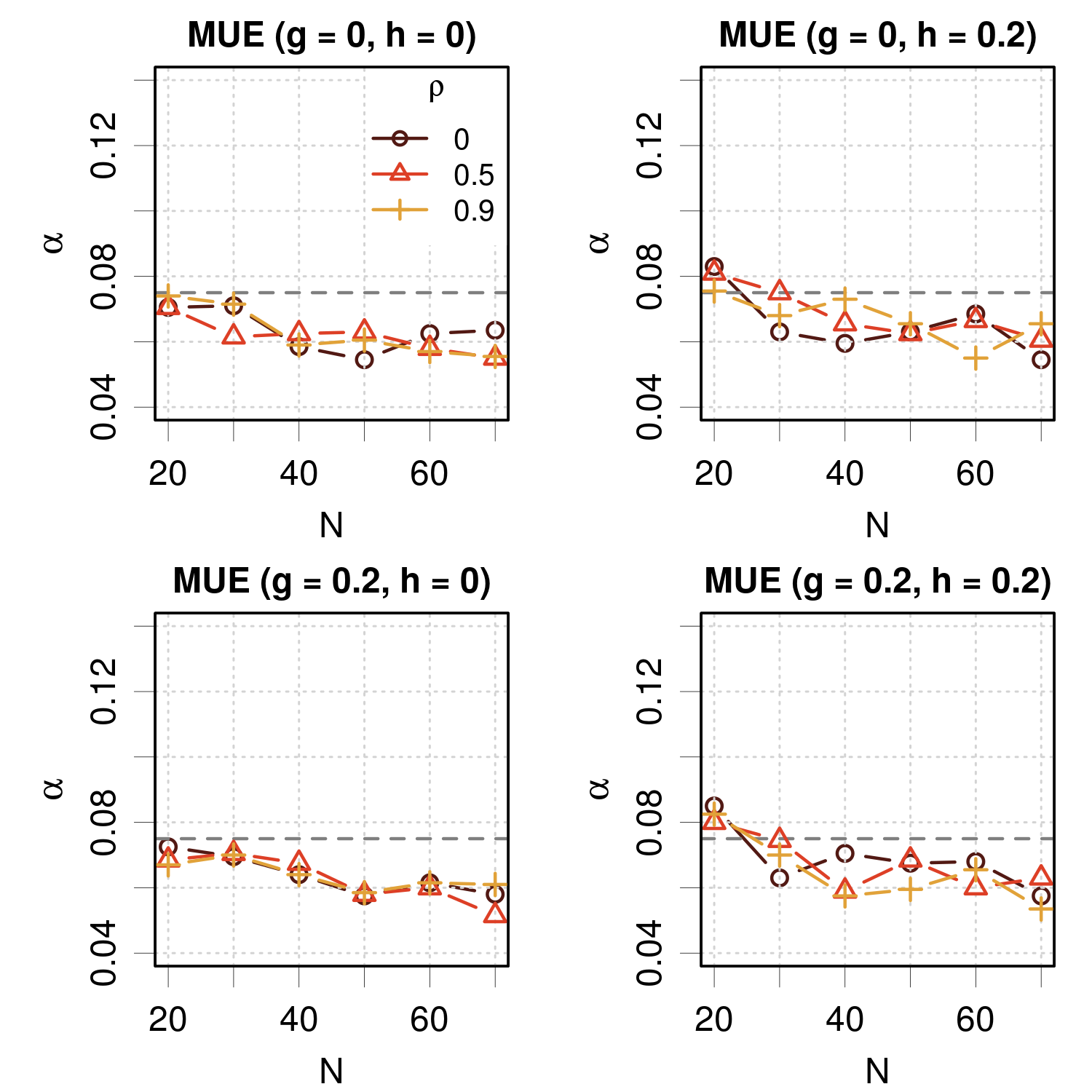
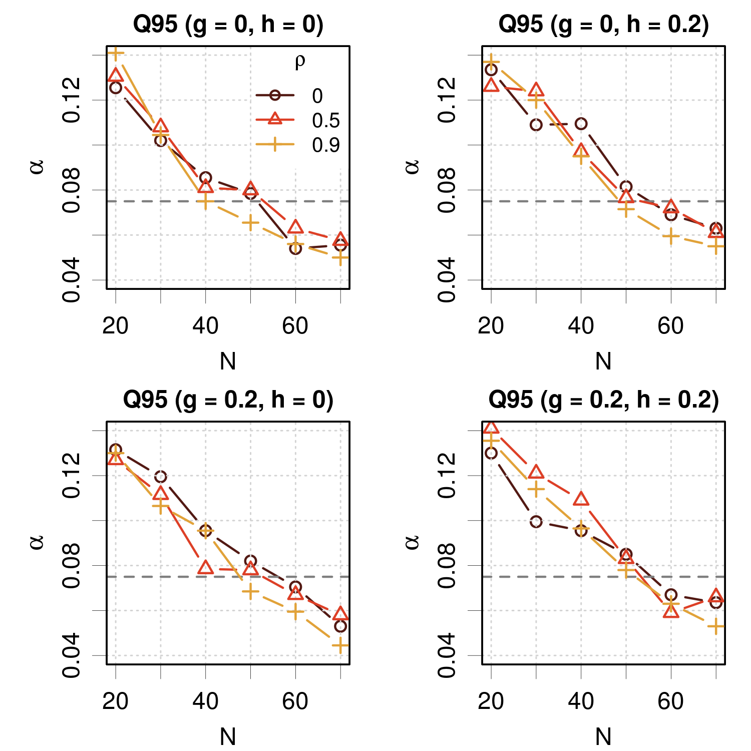
Figure 6: Probability of type I errors $\alpha$ for the MUE (left) and $Q_{95}$ (right), as a function of dataset size $N$. Each graph corresponds to a type of g-and-h distribution for the data samples (see text for details). The points and lines correspond to a value of the datasets correlation coefficient $\rho$. The black dashed line depicts the upper safety limit (0.075).

For the MUE, the safety region ($\alpha\leq 0.075$; black dashed line) (Bradley1978, ) is reached in all cases for $N\geq 30$. Above $N=40$, all values of $\alpha$ are close to the nominal value (0.05). There is no remarkable trend with respect to the type of g-and-h distribution, nor the correlation coefficient. We have estimated previously (Pernot2018, ) that the MUE is typically located between the 0.5 and 0.75 quantiles, for which Wilcox and Erceg-Hurn (Wilcox2012, ) have concluded that the minimal dataset size is $N\geq 30$, which is confirmed here.

For $Q_{95}$, one sees that for $N=40$, the situation is more favorable for the normal distribution, but in all cases, the recommended limit is reached for $N\geq 60$. Strong correlation coefficients ($\rho=0.9$) seem also to be more favorable, and one observes a slight deleterious effect below $N=50$ for heavy-tailed distributions ($h=0.2$). Nevertheless, even for $N=30$, $\alpha$ does not exceed notably 12 % probability of type I error.

Remark.

Establishing the power of the test ($1-\beta$), where $\beta$ is the probability of type II errors (false negative, or the non-rejection of a false null hypothesis)(Gregory05a, ) requires the definition an alternative hypothesis (Klauenberg2019a, ). In the present case, there is a infinity of ways to realize the $s_{1}\neq s_{2}$ alternative, so the power estimation is practically intractable.

Appendix D Numerical study of the Harrell and Davis algorithm

This example is intended to outline the advantages of Harrell and Davis (HD) algorithm for quantiles estimation, notably when associated with bootstrap sampling, as suggested by Wilcox and Erceg-Hurn (Wilcox2012, ).

One considers the values $s_{1}$ and $s_{2}$ of a statistic $S$ for two datasets $E_{1}$ and $E_{2}$, which are drawn from a bivariate normal distribution

$$(E_{1},E_{2})\sim\mathcal{N}\left(\boldsymbol{\mu}=(\mu_{1},\mu_{2}),\boldsymbol{\Sigma}=\left(\begin{array}[]{cc}\sigma_{1}^{2}&\rho\sigma_{1}\sigma_{2}\\ \rho\sigma_{1}\sigma_{2}&\sigma_{2}^{2}\end{array}\right)\right)$$ (43)

where the error samples have different means $(\mu_{1},\mu_{2})$ and variances $(\sigma_{1}^{2},\sigma_{2}^{2})$, and $\mathrm{cov}(E_{1},E_{2})=\rho\sigma_{1}\sigma_{2}$. The values of the parameters for the simulations and the corresponding statistics are given in Table 1. The reference values for the MUE and $Q_{95}$ are obtained as described in a previous article (Pernot2018, ), based on the properties of the folded normal distribution.

Set		MSE	RMSD	MUE	$Q_{95}$
$E_{1}$		0	1.1	0.88	2.16
$E_{2}$		0.1	1.0	0.80	1.97

Table 1: Reference values for the univariate statistics of datasets $E_{1}$ and $E_{2}$ described by Eq. 43, for $\mu_{1}=0$, $\mu_{2}=0.1$, $\sigma_{1}=1.1$ and $\sigma_{2}=1.0$.

D.1 Comparison of HD and $\hat{Q}_{7}$ quantiles

$Q_{95}$ is estimated by two algorithms: the HD algorithm and the $\hat{Q}_{7}$ method of Hyndman and Fan (Hyndman1996, ), which is the default algorithms in the quantile() function of R (CiteR, ). $\hat{Q}_{7}$ is one of a family of quantile estimators based on the linear combination of one or two order statistics (Hyndman1996, ), whereas the HD algorithm is based on the linear combination of all order statistics for a sample (Harrell1982, ). The latter is more efficient for small samples, but more computationally demanding (Harrell1982, ).

In a first test, data sets of increasing sizes, between $N=20$ and 500, are generated by random sampling from the normal distribution for $E_{2}$, and $Q_{95}$ is estimated for each sample by both algorithms. This procedure is repeated $10^{4}$ times, and the distributions of $Q_{95}$ values are summarized by a set of five quantiles (0.05, 0.25, 0.5, 0.75, 0.95). The results are presented in Fig. 7(a). This simulation shows that the HD quantiles converge faster to the true value (1.97) than the $\hat{Q}_{7}$ ones, with less bias for small samples ($N<100$).

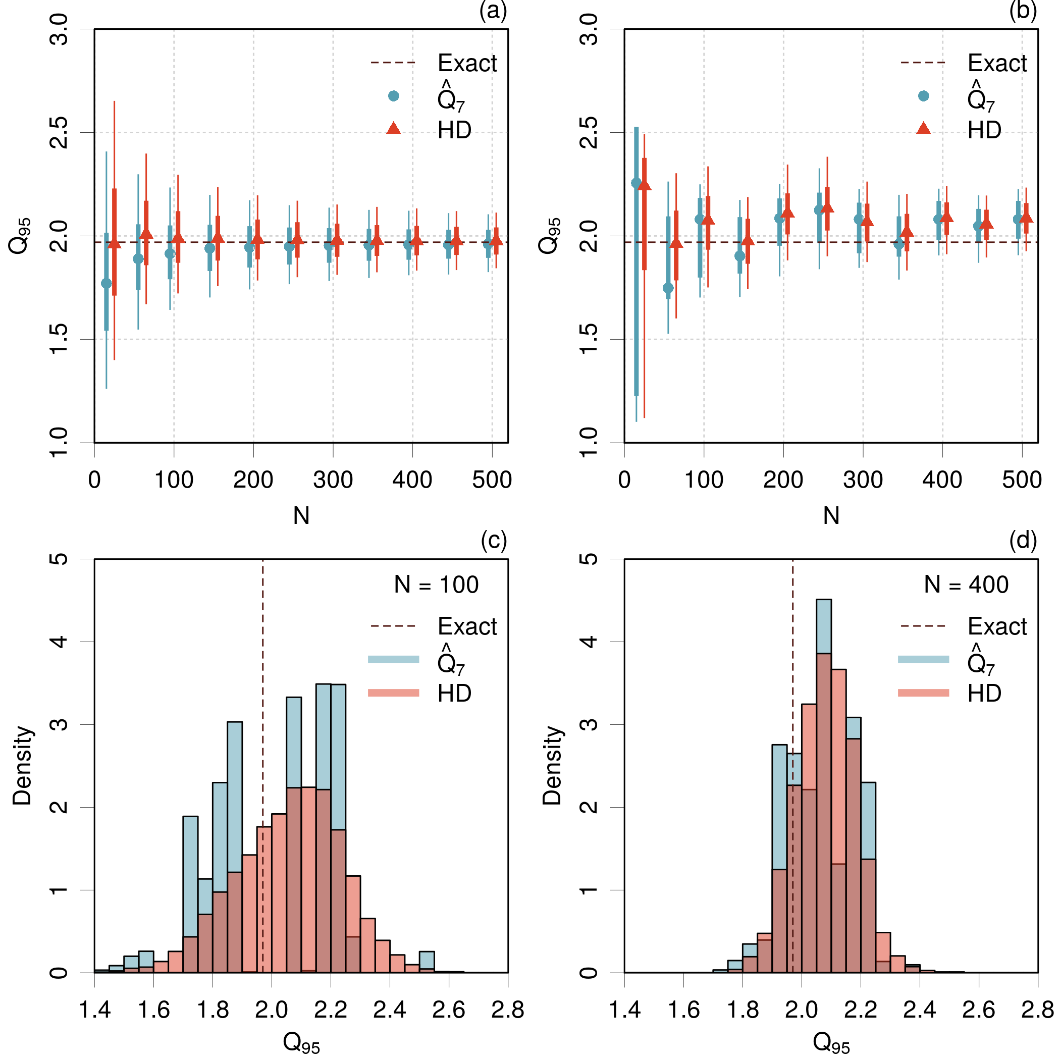
Figure 7: Comparison of $Q_{95}$ estimation algorithms, $\hat{Q}_{7}$ and HD: (a) Monte Carlo sampling; (b) bootstrap sampling; (c) bootstrap sample histogram for $N=100$; (d) idem for $N=400$. The thicker bars in (a,b) represent 25-75 % probability intervals and the finer bars 5-95 % probability intervals. The black dashed line represents the theoretical value for $Q_{95}$ (1.97).

In a second test, a unique $E_{2}$ sample of size $N=500$ is generated, and subsets of increasing size are taken as initial data for a bootstrap procedure ($10^{4}$ repeats). The bootstrap samples are analyzed as above and plotted in Fig. 7(b). The difference of convergence between both quantile algorithms is less striking, but bootstrap for the $\hat{Q}_{7}$ algorithm seems to produce very asymmetric distributions, where the median is close to one of the quartiles. If one looks at the histograms of sampled values for $N=100$ (Fig. 7(c)), one sees that the HD algorithms produces a much smoother bootstrap sample histogram, where $\hat{Q}_{7}$ produces a ragged histograms. The same features are still visible, to a lesser extent, for $N=400$ (Fig. 7(d)). This property of the HD method explains its good performances for small samples, when used in conjunction with the bootstrap (Wilcox2012, ).

D.2 Estimation of $p$-values

The estimation of $p$-values is obtained by Monte Carlo sampling of $E_{1}$ and $E_{2}$ sets of size $N$ varying between 20 and 500 ($\rho=0.9$). One first checks that the generalized $p$-value $p_{g}$ (Algorithm 1) is identical to the analytical value of $p_{t}$ for the comparison of mean values (Fig. 8(a)).

Then, the interest of the Harrell-Davis algorithm for the estimation of $p_{g}$ values for the comparison of quantiles is shown in Fig. 8(b): reaching the 0.05 threshold requires about 250 points for the HD method, whereas the $\hat{Q}_{7}$ reference quantile algorithm requires about 380 points. Besides, the HD curve is smoother than the reference one, due to the smoothness properties of the HD estimator shown above.

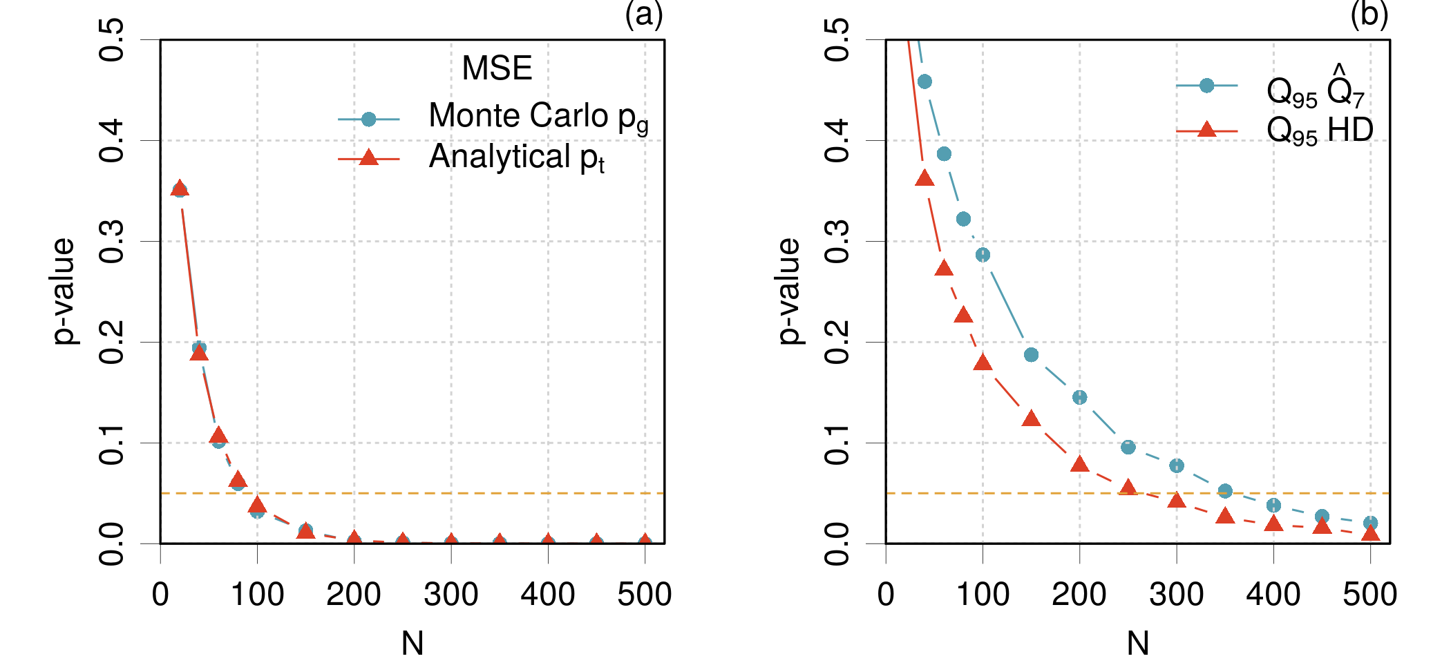
Figure 8: Validation of methodological choices for $p$-value estimation: (a) generalized $p$-value $p_{g}$ for the comparison of means (MSE) compared to the analytical result $p_{t}$ ; (b) impact of the quantile estimation algorithm on $p_{g}$ for the comparison of $Q_{95}$ values. See text for details about the HD and $\hat{Q_{7}}$ algorithm.

Appendix E The g-and-h distribution

The g-and-h distribution (Hoaglin1985, ) is typically used to study the impact of distribution shapes on statistics. If $z$ has a standard normal distribution, its transform

$$X=\begin{cases}\frac{1}{g}(e^{gz}-1)e^{\frac{h}{2}z^{2}},&\mathrm{if}\thinspace g>0\\ ze^{\frac{h}{2}z^{2}}&\mathrm{if}\thinspace g=0\end{cases}$$ (44)

has a g-and-h distribution. Its shape is defined by parameters $g$ and $h$, and contains the normal distribution as a special case ($g=h=0$). Besides the normal, three typical cases are proposed by Wilcox and Erceg-Hurn (Wilcox2012, ): heavy-tailed symmetric ($g=0;\thinspace h=0.2$), light-tailed asymmetric ($g=0.2;\thinspace h=0$), and heavy-tailed asymmetric ($g=h=0.2$).

References

- (1) R. A. Mata and M. A. Suhm. Benchmarking quantum chemical methods: Are we heading in the right direction? Angew. Chem. Int. Ed., 56(37):11011–11018, 2017. doi:10.1002/anie.201611308.
- (2) B. Civalleri, D. Presti, R. Dovesi, and A. Savin. On choosing the best density functional approximation. In Chemical Modelling: Applications and Theory, volume 9, pages 168–185. Royal Soc. Chem., 2012. doi:10.1039/9781849734790-00168.
- (3) P. Pernot and A. Savin. Probabilistic performance estimators for computational chemistry methods: the empirical cumulative distribution function of absolute errors. J. Chem. Phys., 148:241707, 2018. doi:10.1063/1.5016248.
- (4) We argued that is more informative than the MUE, because the latter provides probabilistic information only if the errors distribution is zero-centered normal, a rather unlikely occurrence. In contrast, gives us the error level that one has only 5\tmspace+.1667em% chance to exceed in a new calculation (provided that the reference dataset is representative of the systems for which predictions are sought). The end-users can easily check if this threshold meets their expectations. We recently realized that the 90th percentile (noted ) has been used by Thakkar and colleagues in the same spirit (Thakkar2015, ; Wu2015b, ). We think is more appropriate because of its direct link to the enlarged uncertainty recommended in the thermochemistry literature (Ruscic2014, ; Pernot2018, ).
- (5) T. Gould. ’Diet GMTKN55’ offers accelerated benchmarking through a representative subset approach. Phys. Chem. Chem. Phys., 20:27735–27739, 2018. doi:10.1039/C8CP05554H.
- (6) P. Morgante and R. Peverati. Statistically representative databases for density functional theory via data science. Phys. Chem. Chem. Phys., 21:19092–19103, 2019. doi:10.1039/C9CP03211H.
- (7) R. Ramakrishnan, P. O. Dral, M. Rupp, and O. A. von Lilienfeld. Big data meets quantum chemistry approximations: The -machine learning approach. J. Chem. Theory Comput., 11:2087–2096, 2015. doi:10.1021/acs.jctc.5b00099.
- (8) P. Zaspel, B. Huang, H. Harbrecht, and O. A. von Lilienfeld. Boosting quantum machine learning models with a multilevel combination technique: Pople diagrams revisited. J. Chem. Theory Comput., 15(3):1546–1559, 2019. doi:10.1021/acs.jctc.8b00832.
- (9) J. Proppe and M. Reiher. Reliable estimation of prediction uncertainty for physicochemical property models. J. Chem. Theory Comput., 13:3297–3317, 2017. doi:10.1021/acs.jctc.7b00235.
- (10) A. Nicholls. Confidence limits, error bars and method comparison in molecular modeling. Part 2: comparing methods. J. Comput.-Aided Mol. Des., 30:103–126, 2016. doi:10.1007/s10822-016-9904-5.
- (11) P. Pernot and A. Savin. Probabilistic performance estimators for computational chemistry methods: Systematic improvement probability and ranking probability matrix. II. Applications. arXiv:2003.01572, 2020. URL: https://arxiv.org/abs/2003.01572.
- (12) BIPM, IEC, IFCC, ILAC, ISO, IUPAC, IUPAP, and OIML. Evaluation of measurement data - Guide to the expression of uncertainty in measurement (GUM). Technical Report 100:2008, Joint Committee for Guides in Metrology, JCGM, 2008. URL: http://www.bipm.org/utils/common/documents/jcgm/JCGM_100_2008_F.pdf.
- (13) P. P. Janes and A. P. Rendell. Placing rigorous bounds on numerical errors in Hartree–Fock energy computations. J. Chem. Theory Comput., 7:1631–1639, 2011. doi:10.1021/ct200026t.
- (14) Cancès, Eric and Dusson, Geneviève. Discretization error cancellation in electronic structure calculation: toward a quantitative study. ESAIM: M2AN, 51:1617–1636, 2017. doi:10.1051/m2an/2017035.
- (15) P. J. Reynolds, D. M. Ceperley, B. J. Alder, and W. A. Lester. Fixed-node quantum Monte Carlo for molecules. J. Chem. Phys., 77:5593–5603, 1982. doi:10.1063/1.443766.
- (16) F. Cailliez and P. Pernot. Statistical approaches to forcefield calibration and prediction uncertainty of molecular simulations. J. Chem. Phys., 134:054124, 2011. doi:10.1063/1.3545069.
- (17) J. J. Mortensen, K. Kaasbjerg, S. L. Frederiksen, J. K. Nørskov, J. P. Sethna, and K. W. Jacobsen. Bayesian error estimation in density-functional theory. Phys. Rev. Lett., 95:216401, Nov 2005. doi:10.1103/PhysRevLett.95.216401.
- (18) P. Pernot. The parameter uncertainty inflation fallacy. J. Chem. Phys., 147(10):104102, September 2017. doi:10.1063/1.4994654.
- (19) D. Bakowies. Estimating systematic error and uncertainty in ab initio thermochemistry. I. Atomization energies of hydrocarbons in the ATOMIC(hc) protocol. J. Chem. Theory Comput., 15:5230–5251, 2019. doi:10.1021/acs.jctc.9b00343.
- (20) D. Bakowies. Estimating systematic error and uncertainty in ab initio thermochemistry: II. ATOMIC(hc) enthalpies of formation for a large set of hydrocarbons. J. Chem. Theory Comput., 2020. doi:10.1021/acs.jctc.9b00974.
- (21) G. W. Snedecor and W. G. Cochran. Statistical Methods, Eighth edition. Iowa State University Press, 1989.
- (22) D. J. Murdoch and E. D. Chow. A graphical display of large correlation matrices. Am. Stat., 50(2):178–180, 1996. doi:10.1080/00031305.1996.10474371.
- (23) P. Pernot, B. Civalleri, D. Presti, and A. Savin. Prediction uncertainty of density functional approximations for properties of crystals with cubic symmetry. J. Phys. Chem. A, 119:5288–5304, 2015. doi:10.1021/jp509980w.
- (24) S. De Waele, K. Lejaeghere, M. Sluydts, and S. Cottenier. Error estimates for density-functional theory predictions of surface energy and work function. Phys. Rev. B, 94:235418, 2016. doi:10.1103/PhysRevB.94.235418.
- (25) B. Efron. Bootstrap Methods: Another Look at the Jackknife. Ann. Stat., 7(1):1–26, January 1979. doi:10.1214/aos/1176344552.
- (26) B. Efron and R. Tibshirani. Statistical data analysis in the computer age. Science, 253:390–395, 1991. doi:10.1126/science.253.5018.390.
- (27) T. C. Hesterberg. What teachers should know about the bootstrap: Resampling in the undergraduate statistics curriculum. Am. Stat., 69:371–386, 2015. doi:10.1080/00031305.2015.1089789.
- (28) I. BIPM, I. IFCC, I. ISO, and O. IUPAP. Evaluation of measurement data – supplement 2 to the ’guide to the expression of uncertainty in measurement’ – extension to any number of output quantities. JCGM, 102, 2011.
- (29) R. N. Kacker, R. Kessel, and K.-D. Sommer. Assessing differences between results determined according to the guide to the expression of uncertainty in measurement. J. Res. Nat. Inst. Stand. Technol., 115(6):453, 2010. doi:10.6028/jres.115.031.
- (30) F. C. Leone, L. S. Nelson, and R. B. Nottingham. The Folded Normal Distribution. Technometrics, 3:543–550, 1961. doi:10.1080/00401706.1961.10489974.
- (31) A. Nicholls. Confidence limits, error bars and method comparison in molecular modeling. Part 1: The calculation of confidence intervals. J. Comput.-Aided Mol. Des., 28:887–918, 2014. doi:10.1007/s10822-014-9753-z.
- (32) R. Y. Liu and K. Singh. Notions of limiting -values based on data depth and bootstrap. J. Am. Stat. Assoc., 92:266–277, 1997. URL: http://www.jstor.org/stable/2291471, doi:10.2307/2291471.
- (33) R. R. Wilcox and D. M. Erceg-Hurn. Comparing two dependent groups via quantiles. J. App. Stat., 39:2655–2664, 2012. doi:10.1080/02664763.2012.724665.
- (34) P. Hall, H. Miller, et al. Using the bootstrap to quantify the authority of an empirical ranking. Ann. Stat., 37:3929–3959, 2009. doi:10.1214/09-AOS699.
- (35) A summary in results tables can also be considered, by reporting for each method its mode in ranking probability and the corresponding probability, which indicates the strength of this rank.
- (36) R Core Team. R: A Language and Environment for Statistical Computing. R Foundation for Statistical Computing, Vienna, Austria, 2019. Version 3.6.1. URL: https://www.R-project.org/.
- (37) A. Canty and B. Ripley. boot: Bootstrap Functions (Originally by Angelo Canty for S), 2019. R package version 1.3-22. URL: https://CRAN.R-project.org/package=boot.
- (38) F. E. Harrell and C. Davis. A new distribution-free quantile estimator. Biometrika, 69:635–640, 1982. doi:10.2307/2335999.
- (39) R. R. Wilcox and G. A. Rousselet. A guide to robust statistical methods in neuroscience. Curr. Prot. Neuroscience, 82:8.42.1–8.42.30, 2018. doi:10.1002/cpns.41.
- (40) P. Mair and R. Wilcox. WRS2: A Collection of Robust Statistical Methods, 2019. R package version 1.0-0. URL: https://CRAN.R-project.org/package=WRS2.
- (41) P. Pernot and A. Savin. Codes and data that support the findings of this study, 2020. doi:10.5281/zenodo.3678481.
- (42) Note that in Eq.\tmspace+.1667em34 does not account for the uncertainty on . Taking this factor into account leads to a larger uncertainty, which can be estimated as (Kacker2003, ). This formula is based on the properties of the Student’s-t distribution (Evans2000, ). The impact of the correction factor is notable only for very small datasets (smaller than 3\tmspace+.1667em% for ), and we will consider the standard formula .
- (43) P. R. Bevington and D. K. Robinson. Data Reduction and Error Analysis for the Physical Sciences. McGraw-Hill, New York, 1992.
- (44) R. N. Kacker. Combining information from interlaboratory evaluations using a random effects model. Metrologia, 41:132–136, 2004. doi:10.1088/0026-1394/41/3/004.
- (45) A. L. Rukhin. Weighted means statistics in interlaboratory studies. Metrologia, 46:323, 2009. doi:10.1088/0026-1394/46/3/021.
- (46) C. Rivier, M. Désenfant, M. Crozet, C. Rigaux, D. Roudil, B. Tufféry, and A. Ruas. Use of an excess variance approach for the certification of reference materials by interlaboratory comparison. Accredit. Qual. Assur., 19:269–274, 2014. doi:10.1007/s00769-014-1066-3.
- (47) K. Lejaeghere, J. Jaeken, V. V. Speybroeck, and S. Cottenier. Ab initio based thermal property predictions at a low cost: An error analysis. Phys. Rev. B, 89:014304, jan 2014. doi:10.1103/physrevb.89.014304.
- (48) K. Lejaeghere, V. Van Speybroeck, G. Van Oost, and S. Cottenier. Error estimates for solid-state density-functional theory predictions: An overview by means of the ground-state elemental crystals. Crit. Rev. Solid State Mater. Sci., 39:1–24, 2014. doi:10.1080/10408436.2013.772503.
- (49) Note that the dispersion of model errors is related to the model prediction uncertainty and is a score of interest for the ranking of models (Pernot2015, ; Pernot2018, ).
- (50) P. C. Gregory. Bayesian logical data analysis for the physical sciences. Cambridge University Press, Cambridge, UK, 2005.
- (51) K. Klauenberg and C. Elster. Testing normality. tm - Technisches Messen, 86:773–783, 2019. doi:10.1515/teme-2019-0148.
- (52) J. V. Bradley. Robustness? Br. J. Math. Stat. Psychol., 31(2):144–152, 1978. doi:10.1111/j.2044-8317.1978.tb00581.x.
- (53) R. R. Wilcox. WRS: A Package of R.R. Wilcox’ Robust Statistics Functions, 2019. R package version 0.36.
- (54) R. J. Hyndman and Y. Fan. Sample quantiles in statistical packages. Am. Stat., 50:361–365, 1996. doi:10.2307/2684934.
- (55) D. C. Hoaglin. Exploring data tables, trends, and shapes, chapter Summarizing shape numerically: The g-and-h distributions, pages 461–513. Wiley, New York, 1985.
- (56) A. J. Thakkar and T. Wu. How well do static electronic dipole polarizabilities from gas-phase experiments compare with density functional and MP2 computations? J. Chem. Phys., 143:144302, 2015. doi:10.1063/1.4932594.
- (57) T. Wu, Y. N. Kalugina, and A. J. Thakkar. Choosing a density functional for static molecular polarizabilities. Chem. Phys. Lett., 635:257–261, 2015. doi:10.1016/j.cplett.2015.07.003.
- (58) B. Ruscic. Uncertainty quantification in thermochemistry, benchmarking electronic structure computations, and active thermochemical tables. Int. J. Quantum Chem., 114:1097–1101, 2014. doi:10.1002/qua.24605.
- (59) R. Kacker and A. Jones. On use of bayesian statistics to make the Guide to the Expression of Uncertainty in Measurement consistent. Metrologia, 40:235–248, 2003. doi:10.1088/0026-1394/40/5/305.
- (60) M. Evans, N. Hastings, and B. Peacock. Statistical Distributions. Wiley-Interscience, 3rd edition, 2000.