Hyper-Differential Sensitivity Analysis for Inverse Problems Constrained by Partial Differential Equations

Abstract

High fidelity models used in many science and engineering applications couple multiple physical states and parameters. Inverse problems arise when a model parameter cannot be determined directly, but rather is estimated using (typically sparse and noisy) measurements of the states. The data is usually not sufficient to simultaneously inform all of the parameters. Consequently, the governing model typically contains parameters which are uncertain but must be specified for a complete model characterization necessary to invert for the parameters of interest. We refer to the combination of the additional model parameters (those which are not inverted for) and the measured data states as the“complementary parameters”. We seek to quantify the relative importance of these complementary parameters to the solution of the inverse problem. To address this, we present a framework based on hyper-differential sensitivity analysis (HDSA). HDSA computes the derivative of the solution of an inverse problem with respect to complementary parameters. We present a mathematical framework for HDSA in large-scale PDE-constrained inverse problems and show how HDSA can be interpreted to give insight about the inverse problem. We demonstrate the effectiveness of the method on an inverse problem by estimating a permeability field, using pressure and concentration measurements, in a porous medium flow application with uncertainty in the boundary conditions, source injection, and diffusion coefficient.

Keywords: Inverse Problems, sensitivity analysis, model uncertainty, design of experiments, subsurface flow.

1 Introduction

Rapid advances in numerical algorithms and computing infrastructure have made it feasible to simulate complex multiphysics systems governed by systems of partial differential equations (PDEs) on high resolution computational grids. Inverse problems arise when some model parameters cannot be determined directly, but rather are estimated using measurements of the model state variables. The states may correspond to different physical quantities with varying data volumes and measurement fidelities, and measurements are typically sparse and noisy due to budget and hardware limitations.

Inverse problems governed by systems with complex physics involve various sources of uncertainty. This includes the uncertainty in the parameters being estimated, uncertainty in measurement data, and uncertainty in parameters in governing PDEs that are not the focus of the parameter estimation, but are needed for a full model specification. For clarity, we refer to the model parameters being estimated as inversion parameters and to the other model parameters besides the inversion parameter as auxiliary parameters. Additionally, we refer to the parameters specifying the experimental conditions, such as types of measurements or measurement noise levels, as experimental parameters. The auxiliary parameters and the experimental parameters are needed for the formulation of the inverse problem. We call the combination of auxiliary and experimental parameters the complementary parameters. This article is about understanding and quantifying the impact and relative importance of the perturbations in complementary parameters to the solution of an inverse problem.

For illustration, let us consider a subsurface flow problem, in which we seek to invert for the log-permeability field using a tracer test. The forward model we consider is given by the mass conservation, constrained by Darcy’s law, resulting in a linear elliptic PDE governing the pressure, and a time-dependent PDE governing diffusion and transport of the tracer. The inversion parameter here is the log-permeability field. The auxiliary parameters include the source terms (e.g., the tracer injection), boundary conditions, and coefficients (e.g., the diffusion coefficient) in the governing PDE system. The measurements correspond to the two states: pressure and concentration. The experimental parameters correspond to noise in these measurements.

We propose a general framework to assess the relative importance of complementary parameters in determining the solution of the inverse problem. To do so, we build upon previous work in [1], and a series of related articles [2, 3, 4, 5, 6, 7, 8, 9], that introduced hyper-differential sensitivity analysis (HDSA) for PDE-constrained optimization. HDSA computes the Fréchet derivative of the solution of the inverse problem with respect to complementary parameters. We use this derivative to define hyper-differential sensitivities of the inverse problem solution with respect to the complementary parameters. These sensitivities describe the change in the solution of the inverse problem with respect to perturbations of a given parameter. We also define generalized sensitivity indices that determine maximum (worst case) changes in the inverse problem solution with respect to perturbations in a set of complementary parameters.

By providing sensitivity information on the experimental parameters, our framework provides vital information for effective data collection. For instance, by discovering the sensor measurements the inverse problem solution is most sensitive to, we can identify the sensors where higher fidelity measurements are desired. This can be achieved by designing sensors with improved error tolerances, or in problems where this is possible, repeating these sensor measurements to reduce the associated measurement noise. Furthermore, we demonstrate that HDSA can be used to compare the relative importance of different types of sensors. As such, this process complements experimental design which is used to design optimal sensor placement for data measurements. By calibrating the measurement fidelities in a given experimental design (e.g., a sensor network), one can make the most out of the measurements for effective parameter estimation. Therefore, the proposed framework can be combined with an optimal experimental design (OED) problem [10, 11, 12] to: (i) identify an optimal set of experiments; and (ii) calibrate the fidelities of the experiments or further prune the specified set of experiments, based on the sensitivity analysis results. HDSA provides a systematic framework to distinguish between measurements obtained from different sensor types and understand the relative importance of spatial and temporal sensor distributions. While HDSA is not intended to replace OED, it augments it by providing unique insights into the influence of various sensors in large-scale multiphysics applications.

Another important application of the proposed framework is guiding OED under uncertainty. In practical applications, an OED problem must be found in such a way that it is robust with respect to uncertainty in auxiliary model parameters; see e.g., [13]. Performing sensitivity analysis of the inverse problem solution with respect to auxiliary parameters informs the sources of model uncertainty one needs to focus on when solving an OED under uncertainty problem. By focusing on sources of model uncertainty the inverse problem solution is most sensitive to, our framework can significantly reduce the complexity of an OED under uncertainty problem. Furthermore, for applications in which multiple experiments may be designed to target calibration of different auxiliary parameters, the proposed sensitivities may identify where experimental efforts should be invested to calibrate the most influential parameters through a sequence of different experiments.

Additionally, in complex physics systems, typically the influence of various sources of model uncertainty on the solution behavior is not clear a priori. The proposed sensitivity analysis framework provides important insight about the governing model.

In contrast to traditional sensitivity analysis, where one quantifies the contribution of auxiliary parameters to variability in model output, our proposed framework provides a goal oriented sensitivity analysis approach by quantifying the impact of perturbations in auxiliary parameters on estimation of unknown model parameters. This enables determining which auxiliary parameters need to be specified more accurately. In fact, it might be that some auxiliary parameters should be estimated along with the inversion parameters, if possible.

Lastly, these sensitivities provide a computationally efficient low order approach to uncertainty quantification for large-scale systems. For instance, if the solution of the inverse problem must be determined in real time to inform critical decision making, coupling the estimated solution with a notion of uncertainty contributed by errors in the complementary parameters provides real time uncertainty estimation which is critical for making informed decisions.

The present work concerns local sensitivity analysis for deterministic variational inverse problems. We consider connections to statistical formulations and global sensitivity analysis in Section 7. The contributions of this article are as follows:

• We define HDSA with respect to experimental parameters. This provides a systematic approach to compare different sensor types and reveals information about the relative importance of distributed (spatially and temporally) sensor measurements, neither of which can be easily determined by traditional OED.

• Theoretical results are presented for linear inverse problems to provide intuition and demonstrate properties of the sensitivities with respect to experimental parameters.

• We build upon previous work [1] to develop a more comprehensive mathematical framework for HDSA of nonlinear multiphysics inverse problems. This is done, in particular, by maturing the idea of generalized sensitivities as a tool for systematically comparing the importance of auxiliary parameters (which may be of differing physical characteristics and scales) alongside the novel development of HDSA for experimental parameters.

• Comprehensive numerical results, in a large-scale subsurface flow application, demonstrate the interpretation and use of HDSA for nonlinear multiphysics inverse problems.

The remainder of the article is organized as follows. Section 2 outlines the basic principles of inverse problems and design of experiments. Section 3 provides the mathematical formulation of hyper-differential sensitivities and their interpretation for inverse problems constrained by multiphysics. The computational considerations, implementation, and cost analysis of HDSA is detailed in Section 4. Section 5 presents a large scale, multiphysics model problem, which is then used to construct sensitivity results that are detailed in Section 6. Concluding remarks and notes on potential areas of future work are highlighted in Section 7.

2 Preliminaries

In this section, we recall background material on inverse problems and design of experiments, which are augmented by the proposed sensitivity analysis in subsequent sections.

2.1 Inverse Problems

In the present work, we are concerned with ill-posed inverse problems governed by PDEs. Specifically, we seek to estimate a parameter $m$, henceforth called the inversion parameter, using data $\boldsymbol{y}$ and a model of the form

$$F(m)+\boldsymbol{\eta}=\boldsymbol{y}.$$

Here $F$ is the parameter-to-observable map and $\boldsymbol{\eta}$ represents measurement noise. Evaluating $F(m)$ requires solving the governing PDEs and extracting the solution at measurement points.

Due to ill-posedness and availability of only sparse noisy measurements, we are led to variational formulations with suitable regularizations. Specifically, we consider an optimization problem of the following form:

$$\min\limits_{u,m}J(u,m,\theta_{e})$$ (1)

s.t. $$v(u,m,\theta_{a})=0$$

$$u\in U,m\in\mathcal{M}.$$

Here, $U$ is an infinite dimensional reflexive Banach space containing the state, $\mathcal{M}$ is a possibly infinite dimensional Hilbert space, $J$ is a regularized data misfit cost functional (we make this precise below), and $v$ represents the constraining PDE system. The experimental parameters, $\theta_{e}$, represent uncertainty in the data, while $\theta_{a}$ are the auxiliary parameters contained in the system of PDEs. Generally, solving this optimization problem produces parameter estimates that are consistent with measurement data and the model. For the remainder of the article, we refer to (1) as the inverse problem.

We mention that an alternative approach to address ill-posed inverse problems is to consider a Bayesian formulation [14]. In this approach, the inversion parameter $m$ is modeled as a random variable, and the goal is to find a distribution law for $m$ that is consistent with measurement data, the model, and a prior distribution of $m$ that models our prior knowledge/beliefs about $m$. In the present work, we restrict our attention to deterministic formulation of inverse problems, as described above.

We assume that the PDE represented by $v$ is uniquely solvable for any admissible $m$ and $\theta_{a}$. This allows us to formulate (1) in reduced space [15]. Letting $\mathcal{A}(m,\theta_{a})$ denote the solution operator for the PDE, i.e. $v(\mathcal{A}(m,\theta_{a}),m,\theta_{a})=0$ for all $m$ and $\theta_{a}$, we define the reduced objective function $\hat{J}(m,\theta_{e},\theta_{a})=J(\mathcal{A}(m,\theta_{a}),m,\theta_{e})$. In this article we focus on objective functions defined as a linear combination of data misfit and regularization, yielding a general form for the inverse problem

$$\min_{m\in\mathcal{M}}\hat{J}(m,\theta_{e},\theta_{a}):=\frac{1}{2}\|\mathcal{Q}\mathcal{A}(m,\theta_{a})-\boldsymbol{y}(\theta_{e})\|^{2}+\alpha\mathcal{R}(m),$$ (2)

where $\boldsymbol{y}(\theta_{e})$ is a vector of measured data (with uncertainty parameterized by $\theta_{e}$), $\mathcal{Q}$ an observation operator that maps the PDE solution to a set of observation locations, ${\mathcal{R}}$ is a regularization operator, and $\alpha$ is a regularization parameter. Traditional approaches to solving inverse problems fix $\theta=(\theta_{e},\theta_{a})$ to a best estimate and solve (2) by optimizing over $m$. Analyzing the influence of $\theta$ on the solution of (2) is the focus of this article.

Besides ill-posedness, such inverse problems are difficult to solve for a number of other reasons. These include having noisy observations, expensive forward PDE solves, tuning multiple experimental and modeling parameters, and optimization in infinite (or large finite) dimensional spaces. Common optimization methods used to tackle such problems include quasi-Newton, inexact Newton-CG, Gauss-Newton, and truncated CG trust region solvers. These optimization problems often require efficient gradient and Hessian computation through adjoint state methods, and repeated large scale linear system solves with Krylov iterative methods. We direct the interested reader to a number of classical inverse problem references [16, 17, 18, 19, 20, 21, 22].

2.2 Design of Experiments

An important aspect of solving an inverse problem is the collection of informative measurement data, which is guided by design of experiments. In our target inversion, this generally corresponds to specifying the locations of the sensors used to collect measurement data and is known as an optimal experimental design (OED) problem [10, 11, 12]. OED for inverse problems governed by differential equations has received significant attention in recent years; see e.g., [23, 24, 25, 26, 27, 28, 29, 30, 31, 32, 33, 34]. An OED problem is typically formulated with a statistical formulation of the inverse problem in mind. An optimal design is one that optimizes the statistical quality of the estimated parameters. Examples include maximizing the expected information gain, leading to a D-optimal design problem, or minimization of average posterior variance, leading to a Bayesian A-optimal design problem.

OED is a powerful tool that is used on a wide variety of problems. It is also a very challenging problem both from mathematical and computational point of view, especially when it comes to nonlinear inverse problems governed by PDEs; see e.g., [31, 33]. The developments in the present work are closely related to OED: while we do not directly solve an OED problem, we address the following relevant questions: (i) which measurements is the solution of an inverse problem most sensitive to? And (ii) which measurement types are most influential to the solution of the inverse problem? The latter is tied to important questions typically not addressed in OED literature: how should multi-purpose sensors that can take different types of measurements be deployed, and how should different sensor types be designed and deployed in an existing experimental design?

3 Hyper-differential Sensitivity Analysis for Inverse Problems

This section is devoted to our proposed framework for hyper-differential sensitivity analysis (HDSA) of PDE-constrained inverse problems. In Subsection 3.1, we detail the mathematical formulation of the operator mapping complementary parameters to solutions of the PDE-constrained inverse problem, and its Fréchet derivative. In Subsection 3.2 the hyper-differential sensitivities are defined, as well as the generalized sensitivity index which is used to compare the importance of sets of complementary parameters with different physical characteristics. Subsection  3.3 presents an analytical result for linear inverse problems which connects the sensitivities to the trace of the covariance in the solution of the inverse problem.

3.1 Mathematical Formulation

HDSA differs from traditional sensitivity analysis in that it determines the sensitivity of the solution of an optimization problem rather than simply a model (which is typically a constraint in the optimization problem). We seek to perform HDSA on (2) to determine the sensitivity of the optimal $m$ to uncertainty in complementary (both experimental and auxiliary) parameters $\theta$ which are fixed when solving (2).

HDSA uses the derivative of the solution of (2) with respect to $\theta$. To formally define HDSA, we assume that $\hat{J}$ is twice continuously differentiable with respect to $(m,\theta)$ and that $m^{\star}$ is a local minimum of (2) for specified complementary parameters $\theta=\theta^{\star}$. Assuming that the Hessian of $\hat{J}$ with respect to $m$, evaluated at $(m^{\star},\theta^{\star})$, is positive definite [1, 2], we can apply the implicit function theorem [35, p. 38] to $\hat{J}_{m}$ (the Fréchet derivative of $\hat{J}$ with respect to $m$), to define a continuously differentiable mapping $\mathcal{F}$ from a neighborhood of $\theta^{\star}$ to a neighborhood of $m^{\star}$,

$$\mathcal{F}:\mathcal{N}(\theta^{\star})\to\mathcal{N}(m^{\star})$$

such that

$$\hat{J}_{m}(\mathcal{F}(\theta),\theta)=0,\quad\text{ for all }\quad\theta\in\mathcal{N}(\theta^{\star}),$$

i.e., $\mathcal{F}$ maps complementary parameters to stationary points of (2). The Fréchet derivative of $\mathcal{F}$ with respect to $\theta$, evaluated at $\theta^{\star}$, is given by

$$\mathcal{D}:=\mathcal{F}_{\theta}(\theta^{\star})=-\mathcal{H}^{-1}\mathcal{B},$$ (3)

where $\mathcal{H}$ is the Hessian of $\hat{J}$ with respect to $m$, evaluated at $m^{\star}$ and $\theta^{\star}$, i.e., $\mathcal{H}:=\hat{J}_{m,m}(m^{\star},\theta^{\star})$, and $\mathcal{B}$ is the Fréchet derivative of $\hat{J}_{m}$ with respect to $\theta$, evaluated at $m^{\star}$ and $\theta^{\star}$, i.e., $\mathcal{B}:=\hat{J}_{m,\theta}(m^{\star},\theta^{\star})$.

An intuitive interpretation of (3) is that once (2) has been solved to optimality for the specified $\theta^{\star}$, we take a perturbation with respect to $\theta$ ($\mathcal{B}$) and apply a Newton step ($-\mathcal{H}^{-1}$) to update the solution of the inverse problem. We interpret $\mathcal{D}\overline{\theta}$ as the sensitivity of the solution of the inverse problem when the complementary parameters are perturbed in the direction $\overline{\theta}$. Note that upon discretization, applying the inverse of $\mathcal{H}$ to a vector requires a large-scale linear solve, which requires many PDE solves.

3.2 Sensitivity Indices

We use (3) to define sensitivity indices that attribute importance to each parameter. To this end, we first formalize assumptions about the parameter space. In general, the complementary parameters $\theta=(\theta_{e},\theta_{a})\in\Theta$ take values in a possibly infinite dimensional space $\Theta=\Theta_{1}\times\Theta_{2}\times...\times\Theta_{K}$, which is a product of $K$ Hilbert spaces. The first $\ell$ parameter spaces contain the experimental parameters $\theta_{e}\in\Theta_{1}\times...\times\Theta_{\ell}$, while the remainder contain the auxiliary parameters $\theta_{a}\in\Theta_{\ell+1}\times...\times\Theta_{K}$. The product space $\Theta$ is equipped with the inner product

$$\langle\theta,\phi\rangle_{\Theta}=\langle\theta_{1},\phi_{1}\rangle_{\Theta_{1}}+\dots+\langle\theta_{K},\phi_{K}\rangle_{\Theta_{K}},\quad\text{ for }\quad\theta,\phi\in\Theta.$$

We are particularly interested in cases where each $\Theta_{k}$, $k=1,2,\dots,K$, may have significantly different physical characteristics. For instance, corresponding to various physical quantities (thermal, fluid, solid, etc.) which have different spatial and temporal dependence.

To better understand spatial and temporal patterns of importance within a particular parameter or data source, we define pointwise sensitivity indices in space and time, and later generalized sensitivities which remove these units. From here on, we use $\mathbf{{\Theta}}$ and $\mathbf{{\Theta}}_{k}$ to denote the discretizations of the possibly infinite dimensional spaces $\Theta$ and $\Theta_{k}$. To respect spatiotemporal structure in discrete data, we use weighted norms corresponding to spatial and/or temporal discretizations. For instance, if $\boldsymbol{\theta}_{k}$ models perturbations of spatiotemporal data measurements then

$$\|\boldsymbol{\theta}_{k}\|_{\mathbf{{\Theta}}_{k}}=\sqrt{\frac{1}{n_{t}n_{s}}\sum_{i=1}^{n_{t}n_{s}}(\theta_{k}^{i})^{2}}$$

where $\theta_{k}^{i}$ denotes the $i^{th}$ component of the vector $\boldsymbol{\theta}_{k}\in\mathbb{R}^{n_{t}n_{s}}$, $n_{s}$ and $n_{t}$ denote the number of spatial and temporal points, respectively.

Upon discretization of (1), we let $\{\boldsymbol{b}_{k}^{1},\boldsymbol{b}_{k}^{2},\dots,\boldsymbol{b}_{k}^{n_{k}}\}$ denote a basis for each parameter space $\mathbf{{\Theta}}_{k}$, where $n_{k}$ is the dimension of $\mathbf{{\Theta}}_{k}$.

We define a basis for $\mathbf{{\Theta}}$ as $\{\boldsymbol{e}^{i}_{k}\}$ for $k=1,\dots,K$ and $i=1,\dots,n_{k}$ where

$$\boldsymbol{e}_{k}^{i}=\begin{pmatrix}\boldsymbol{0}_{1}&\dots&\boldsymbol{0}_{k-1}&\boldsymbol{b}_{k}^{i}&\boldsymbol{0}_{k+1}&\dots&\boldsymbol{0}_{K}\end{pmatrix}^{\top}.$$

We define the pointwise sensitivity indices for $k=1,\dots,K$ and $i=1,\dots,n_{k}$ as,

$$S_{k}^{i}=\frac{\|\mathbf{{D}}\boldsymbol{e}_{k}^{i}\|_{\mathbf{{M}}}}{\|\boldsymbol{e}_{k}^{i}\|_{\mathbf{{\Theta}}}},$$ (4)

where $\mathbf{{D}}$ is the discretized sensitivity operator (3), and $\|\cdot\|_{\mathbf{{M}}}$ is the norm discretized consistently with respect to the norm in $\mathcal{M}$. The pointwise sensitivities measure the change in the solution of the inverse problem with respect to a perturbation of the $k^{th}$ parameter in direction $\boldsymbol{b}_{k}^{i}$. Thus, high sensitivity indicates that errors in the parameter will cause a significant change in the reconstructed solution. This leads to an interpretation of the sensitivities as quantifying the importance of accurately measuring or modeling the parameter.

We would also like to compare sensitivities of various parameters with differing units to determine their importance relative to each other. To do this, we seek to formulate a generalized sensitivity index for a particular set of parameters $\boldsymbol{\theta}_{k}\in\mathbf{{\Theta}}_{k}$, which can be interpreted as the maximum change in the solution with respect to a unit norm perturbation of the $k^{th}$ parameter. Care must be taken here to ensure the sensitivities can be compared accurately, as some parameters may be local in space and/or time, while others are not. We first consider a projection operator $\mathbf{{T}}_{k}:\mathbf{{\Theta}}\to\mathbf{{\Theta}}$, which zeros out all elements of $\boldsymbol{\theta}$ except those in $\mathbf{{\Theta}}_{k}$. Then the generalized sensitivity for parameters is

$$S_{k}=\max_{\boldsymbol{\theta}\in\mathbf{{\Theta}}}\frac{\|\mathbf{{D}}\mathbf{{T}}_{k}\boldsymbol{\theta}\|_{\mathbf{{M}}}}{\|\boldsymbol{\theta}\|_{\mathbf{{\Theta}}}}.\\$$ (5)

In this way, we obtain a single generalized sensitivity for each set of parameters $\boldsymbol{\theta}_{k}$, $k=1,\dots,K$, which allows for a dimensionless comparison of parameters with different physical characteristics.

3.3 Interpretation of Experimental Parameter HDSA for Linear Inverse Problems

Sensitivity of auxiliary parameters, $\theta_{a}$ in the notation of this article, is a natural concept with a clear physical interpretation. The sensitivity of the solution of the inverse problem to experimental parameters is less intuitive, so we present an analytic result in Proposition 3.1 to provide intuition. For conciseness and clarity in this subsection, we consider only uncertainty in the experimental parameters.

Assume that $\tilde{\boldsymbol{y}}=(\tilde{y}_{1},\tilde{y}_{2},\dots,\tilde{y}_{n})^{\top}$ is a vector of noisy data which may be modeled by a linear parameter-to-observable map $\mathcal{Q}\mathcal{A}$ acting on an unknown parameter $m$. Estimating this unknown $m$ gives rise to a linear inverse problem. To apply HDSA with respect to experimental parameters, we model the data as

$$y_{i}=\tilde{y}_{i}(1+\theta_{e}^{i})\qquad i=1,2,\dots,n,$$

where $(\theta_{e}^{1},\theta_{e}^{2},\dots,\theta_{e}^{n})^{\top}=\boldsymbol{\theta_{e}}\sim N(0,\mathbf{{\Sigma}})$ is a perturbation of the nominal value $\tilde{y}_{i}$, i.e. a noise model. Assuming uncorrelated observations, the noise covariance matrix is $\mathbf{{\Sigma}}=\mathrm{diag}(\sigma_{1}^{2},\ldots,\sigma_{n}^{2})$. An estimate of the inversion parameter can be obtained by solving

$$\min_{m}\hat{J}(m):=\frac{1}{2}\|\mathcal{Q}\mathcal{A}m-\boldsymbol{y}\|_{\mathbf{{\Sigma}}^{-1}}^{2}+\frac{\alpha}{2}\|m\|_{R}^{2}$$ (6)

with $\boldsymbol{\theta_{e}}=0$, i.e. solving a linear least squares problem with the data $\tilde{\boldsymbol{y}}$. The norm in the regularization term is weighted by regularization operator $R:\mathcal{M}\to\mathcal{M}$ which we assume is a self-adjoint, strictly positive linear operator on $\mathcal{M}$ [22].

The estimator $m^{\star}$ obtained from solving (6) is a random variable, due to the random noise in the data. HDSA provides the sensitivity of its solution with respect to $\boldsymbol{\theta_{e}}=(\theta_{e}^{1},\theta_{e}^{2},\dots,\theta_{e}^{n})$. This may be interpreted as the sensitivity of the least squares estimate with respect to the data, a metric to assess the relative importance of the observations. Such sensitivity information can be used to inform sensor designs and measurement tolerances. Proposition 3.1 relates the variance of $m^{\star}$ (with respect to randomness in $\boldsymbol{\theta_{e}}$) to the pointwise sensitivities with respect to data measurements $S^{i}$ as defined in equation (4). Here, we omit the subscript $(K=1)$ on the pointwise sensitivities, as we only consider one type of parameter in this section.

Proposition 3.1.

$\mathrm{Tr}(\mathrm{Cov}(m^{\star}))=\sum_{i=1}^{n}(S^{i})^{2}$, where $\mathrm{Tr}$ denotes the trace of a linear operator and $S^{i}$ is defined as in (4) when $\Theta=\mathbb{R}^{n}$ is equipped with the $\mathbf{{\Sigma}}^{-1}$ weighted norm.

Proof.

Computing the Fréchet derivative of the objective $\hat{J}$ in (6), setting it equal to zero, and solving for $m$ yields the solution of the inverse problem,

$$m^{\star}=(\mathcal{A}^{*}\mathbf{{W}}\mathcal{A}+\alpha R)^{-1}\mathcal{A}^{*}\mathbf{{W}}\boldsymbol{y}=(\mathcal{A}^{*}\mathbf{{W}}\mathcal{A}+\alpha R)^{-1}\mathcal{A}^{*}\mathbf{{W}}(\tilde{\boldsymbol{y}}+\tilde{\mathbf{{Y}}}\boldsymbol{\theta_{e}}),$$

where $\mathcal{A}^{*}$ denotes the adjoint of the linear operator $\mathcal{A}$ and $\tilde{\mathbf{{Y}}}=\text{diag}\Big{(}\tilde{y_{1}},\tilde{y_{2}},\dots,\tilde{y_{n}}\Big{)}$. Computing the Fréchet derivative of $m^{\star}$ with respect to $\boldsymbol{\theta_{e}}$ (which coincides with (3)) yields

$$\mathcal{D}=(\mathcal{A}^{*}\mathbf{{W}}\mathcal{A}+\alpha R)^{-1}\mathcal{A}^{*}\mathbf{{W}}\tilde{\mathbf{{Y}}}.$$

The covariance of the estimator $m^{\star}$ (with respect to randomness in $\boldsymbol{\theta_{e}}$) is

$$\mathrm{Cov}(m^{\star})=\mathrm{Cov}(\mathcal{D}\boldsymbol{\theta_{e}})=\mathcal{D}\mathbf{{\Sigma}}\mathcal{D}^{*}.$$

Therefore,

$$\mathrm{Tr}(\mathrm{Cov}(m^{\star})) =\mathrm{Tr}(\mathcal{D}\boldsymbol{\Sigma}\mathcal{D}^{*})=\mathrm{Tr}(\mathcal{D}^{*}\mathcal{D}\boldsymbol{\Sigma})=\sum_{i=1}^{n}\langle\boldsymbol{e}_{i},\mathcal{D}^{*}\mathcal{D}\mathbf{{\Sigma}}\boldsymbol{e}_{i}\rangle$$

$$=\sum_{i=1}^{n}(\sigma_{i}\|\mathcal{D}\boldsymbol{e}_{i}\|_{\mathcal{M}})^{2}=\sum_{i=1}^{n}(\sigma_{i}\|\boldsymbol{e}_{i}\|_{\mathbf{{\Sigma}}^{-1}}S^{i})^{2}=\sum_{i=1}^{n}(S^{i})^{2},$$

where $\boldsymbol{e}_{i}$ is the $i^{th}$ canonical unit vector in $\mathbb{R}^{n}$. ∎

This result provides useful intuition into the sensitivity indices and indicates that the variance of the inverse problem solution is scaled by the magnitude of the sensitivities with respect to data.

Remark 3.1.

Notice that Proposition 3.1 generalizes naturally to Bayesian linear inverse problems. With a Gaussian prior and likelihood, the solution of the Bayesian linear inverse problem is a Gaussian posterior. With the assumption $\boldsymbol{\theta}_{e}\sim N(0,\mathbf{{\Sigma}})$ on the measurement noise, and an appropriately chosen prior covariance, the maximum a posteriori (MAP) point is equivalent to the solution $m^{\star}$ of the deterministic linear inverse problem. Taking the trace of the MAP point’s covariance we again conclude Proposition 3.1. Note that in the Bayesian setting, we consider the average variance of the MAP estimator as a measure of robustness of this point estimator for the inversion parameter. This is different than the average posterior uncertainty in the parameter given by the trace of the posterior covariance operator.

4 Computational Considerations

We begin our discussion with a simple illustrative example. To highlight the dimensions of the discretized operators and gain insight into the computational complexity of HDSA, we consider a discretized inverse problem with only auxiliary parameters:

$$\min_{\boldsymbol{m}}\hat{J}(\boldsymbol{m}) =\frac{1}{2}\|\mathbf{{Q}}\boldsymbol{u}-\boldsymbol{y}\|_{\mathbf{{W}}}^{2}+\frac{\alpha}{2}\|\boldsymbol{m}\|_{\mathbf{{R}}}^{2}$$ (7)

$$\text{where }\ \mathbf{{L}}(\boldsymbol{m})\boldsymbol{u} =\mathbf{{V}}\boldsymbol{\theta}.$$

where $\mathbf{{Q}}\in\mathbb{R}^{d\times n}$ is an observation operator, $\boldsymbol{u}\in\mathbb{R}^{n}$ the state vector, $\boldsymbol{y}\in\mathbb{R}^{d}$ is the vector of experimental observations, $\mathbf{{W}}\in\mathbb{R}^{d\times d}$ a symmetric weight matrix, $\alpha>0$ a regularization coefficient, $\boldsymbol{m}\in\mathbb{R}^{p}$ the discretized inversion parameter, $\mathbf{{R}}\in\mathbb{R}^{p\times p}$ a symmetric positive definite regularization operator, $\mathbf{{L}}(\boldsymbol{m})\in\mathbb{R}^{n\times n}$ a discretized differential operator, $\boldsymbol{\theta}\in\mathbb{R}^{k}$ the vector of auxiliary parameters, and $\mathbf{{V}}\in\mathbb{R}^{n\times k}$. Note that the discretized state dimension $n$ corresponds to the number of degrees of freedom in the mesh (typically large), and for problems with distributed parameters, $p$ will also have a comparable dimension to $n$ (frequently equal). The dimension of the auxiliary parameters, $k$, can also be large, potentially larger than $n$ when there are multiple distributed auxiliary parameters.

In practice, we compute the action of the gradient and Hessian of $\hat{J}$ using a formal Lagrangian approach where each application of the Hessian requires two linear PDE solves (inverting the matrix $\mathbf{{L}}(m)$). To compute the action of $\mathbf{{D}}$ (the discretization of (3)) on a vector, we require 2 linear solves to apply the matrix $\mathbf{{B}}$ to a vector, and then $2I$ linear solves to apply $\mathbf{{H}}^{-1}$ to the resulting vector, where $I$ is the number of iterations needed by an iterative linear solver. We direct the reader to A, where we demonstrate the adjoint method used to compute the gradient and Hessian of the reduced objective function $\hat{J}$, as well as the operator $\mathbf{{B}}$.

In general, the sensitivity indices (4) and generalized sensitivity indices (5) may be computed in a variety of ways. The efficiency of different approaches depends upon (i) the dimension of the parameter space, (ii) the computational cost of the PDE solves, (iii) the structure of the Fréchet derivative $\mathcal{D}$, and (iv) the available computational resources.

The computational bottleneck when computing (4) and (5) is repeatedly inverting $\mathcal{H}$ (a large linear system solve). In general, we are interested in systems of nonlinear PDEs. For such systems, each application of $\mathcal{H}^{-1}$ requires $2I$ linearized PDE solves, where $I$ is the number of iterations required by the linear solver (such as conjugate gradient). Because HDSA is post-optimality analysis, we do not require solving nonlinear systems repeatedly as in the inverse problem, but rather solving PDEs which are linearized about the solution of the inverse problem.

As introduced in [1], a randomized generalized eigenvalue problem may be formulated to estimate the truncated generalized singular value decomposition (GSVD) of $\mathcal{D}$. When the parameter dimension is large and Fréchet derivative $\mathcal{D}$ is low rank, both (4) and (5) may be efficiently estimated by using the truncated GSVD and leveraging the parallelism of randomized methods. We refer the reader to [1] for additional details.

If $\mathcal{D}$ is not low rank but the parameter dimension and cost per PDE solve is mild, we may compute (4) and (5) directly by applying $\mathcal{D}$ to each basis function in $\Theta$. This does not exploit structure as in the GSVD approach, but it is embarrassingly parallel making it feasible for moderate parameter dimensions.

If $\mathcal{D}$ is not low rank and the parameter dimension or cost per PDE solver prohibits computing (4) and (5) directly, we may still compute (5) using a GSVD. Each generalized sensitivity index corresponds to the leading singular value of $\mathcal{D}$ acting on a projection operator. Since the number of generalized sensitivities are typically small, they may be estimated by using randomized solvers to compute the leading singular value. By exploiting parallelism, this may be done with a modest number of linearized PDE solvers regardless of the spectral decay in $\mathcal{D}$.

5 Model Problem

In this section, we present a multiphysics model problem which is then used in Section 6 to compute hyper-differential sensitivities and demonstrate the usefulness and flexibility of HDSA. As a motivating example, we consider the problem of identifying the permeability field of a porous subsurface region with a tracer substance flowing through the domain. We consider a unit square domain $\Omega$ with boundary $\Gamma=\cup_{i=0}^{3}\Gamma_{i}$, where $\Gamma_{0}$, $\Gamma_{1}$, $\Gamma_{2}$, and $\Gamma_{3}$ denote the bottom, right, top, and left edges of $\Omega$, respectively.

We model subsurface flow of a fluid through a porous medium with Darcy’s Law and consider transport of the tracer through the medium governed by the advection diffusion equation:

$$-\nabla\cdot(e^{m}\nabla p) =0\quad\text{ in }\Omega$$ (8a)

$$c_{t}-\nabla\cdot\Big{(}\epsilon\nabla c\Big{)}+\nabla\cdot\big{(}\boldsymbol{v}c\big{)} =g\quad\text{ in }[0,T]\times\Omega$$ (8b)

$$p =p_{1}\quad\text{on }\Gamma_{1}$$ (8c)

$$p =p_{2}\quad\text{on }\Gamma_{3}$$ (8d)

$$\nabla p\cdot n =0\quad\text{ on }\Gamma_{0}\cup\Gamma_{2}$$ (8e)

$$\nabla c\cdot n =0\quad\text{ on }[0,T]\times\{\Gamma_{0}\cup\Gamma_{1}\cup\Gamma_{2}\cup\Gamma_{3}\}$$ (8f)

$$c(0,\cdot) =0\quad\text{ in }\Omega$$ (8g)

Here $p$ denotes the pressure field, $m$ the log-permeability field of the medium, $\boldsymbol{v}=-e^{m}\nabla p$ the Darcy velocity, $c(t,x)$ the tracer concentration, $\epsilon$ the diffusivity constant, and $g$ the source term of the injected tracer. In the present example, we used $\epsilon=0.025$. For simplicity of notation, the constant fluid viscosity and constant porosity of the medium have been removed from the model. The Dirichlet pressure boundary conditions (on left and right boundaries) are described by non-zero fuctions $p_{1}$ and $p_{2}$. We let $p_{1}$ be greater in magnitude than $p_{2}$, as this pressure difference will drive fluid flow from right to left through the domain,

$$p_{1}(y) =15+\cos(2\pi y)+\frac{1}{2}\cos(4\pi y),$$

$$p_{2}(y) =10+2\cos(2\pi y).$$

The tracer source is described by

$$g(x,y)=\sum_{k=1}^{16}10e^{-100((x-v_{k})^{2}+(y-w_{k})^{2})}$$

where the source injection locations $(v_{k},w_{k})$ are arranged in a $4\times 4$ grid as depicted by the diamonds in Figure 1.

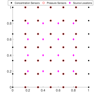
Figure 1: Concentration sensor, pressure sensor, and source locations.

We seek to solve an inverse problem to reconstruct the log-permeability field $m$, using pressure and concentration measurements. Let $\mathcal{Q}$ denote the observation operator and $\boldsymbol{y}\in\mathbb{R}^{n}$ be a vector of $n_{p}$ pressure measurements and $n_{c}$ concentration measurements at $n_{t}$ measurement times, giving a total of $n=n_{p}+n_{c}n_{t}$ data points,

$$\boldsymbol{y}=\begin{bmatrix}p_{1}&p_{2}&\dots&p_{n_{p}}&c_{1}&c_{2}&\dots&c_{n_{c}n_{t}}\end{bmatrix}.$$

The observation (sensor) locations are depicted in Figure 1.

We consider the inverse problem

$$\min_{m}\hat{J}(m):=\ \frac{1}{2}\|\mathcal{Q}\mathcal{A}(m)-\boldsymbol{y}\|_{\mathbf{{W}}}^{2}+\frac{\alpha}{2}\int_{\Omega}\|\nabla m\|_{2}^{2}\ dx$$

where $\mathcal{A}$ is the solution operator for (8),

$$\mathbf{{W}}=\begin{pmatrix}\frac{1}{\overline{p}^{2}\sigma^{2}}\mathbf{{I}}_{n_{p}}&0\\ 0&\frac{1}{\overline{c}^{2}\sigma^{2}}\mathbf{{I}}_{n_{c}n_{t}}\end{pmatrix}$$

is a data misfit weight matrix and $\alpha$ is the regularization coefficient. We used $\alpha=3\times 10^{-2}$ in our numerical experiments; this was chosen based on numerical experimentations seeking a regularization coefficient that is large enough to mitigate ill-posedness and at the same time produces a reasonable parameter reconstruction. The weight matrix divides each measurement by the measurement noise $\sigma$ and the average of its data type ($\overline{p}$ and $\overline{c}$ respectively) to ensure the two data types, which are on different scales, have equivalent importance in the data misfit term.

We synthesize data for this problem with additive Gaussian noise that perturbs the data with a standard deviation of 3$\%$ of the true value, i.e. $\theta_{e}^{i}\sim\mathcal{N}(0,\sigma),\text{ with }\sigma=0.03$. Note that we assume pressure and concentration sensors have the same proportional measurement error, $\sigma_{p}=\sigma_{c}=0.03$.

The inverse problem is solved on a 55$\times$55 finite element spacial discretization with 48 time steps, while the data is generated from a forward PDE solve with a 109$\times$109 finite element spacial discretization and 98 time steps. We use a completely uninformed, constant 0 initial guess, with 49 concentration sensors and 35 pressure sensors arrayed throughout the domain as depicted in Figure 1 to solve the inverse problem.

6 Computational Results

Using the model presented in Section 5, we solve the inverse problem and compute sensitivity indices to determine which parameters and data sources are most important. Figure 2 depicts the true log permeability field we seek to reconstruct through the inverse problem, and the reconstructed solution found by solving the inverse problem with a truncated CG trust region solver. Note that since the optimization problem is non-convex we are only guaranteed to find a local minimizer.

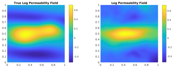
Figure 2: Left: True Permeability     Right: Reconstructed Solution.

In Subsection 6.1 we display and interpret generalized sensitivity indices for the pressure data, concentration data, tracer source term, diffusion coefficient, and the left and right pressure Dirichlet boundary conditions. In Subsection 6.2 we analyze the pointwise sensitivities with respect to the experimental parameters (pressure and concentration data), and in Subsection 6.3 we analyze the pointwise sensitivities with respect to auxiliary parameters (source term, pressure Dirichlet boundary conditions, and diffusion coefficient). General discussion of the importance and interpretation of the sensitivities is presented in Subsection 6.4.

We model uncertain parameters as a nominal value times a parameterized perturbation. When our parameters of interest are constants, such as data measurements or modeling coefficients, we can model uncertain parameters as

$$d=\tilde{d}(1+a\theta),$$

where $d$ is the parameter of interest, $\tilde{d}$ is the nominal value, $a$ is a scaling coefficient, and $\theta\in[-1,1]$ the parameterization of the perturbation. In practice, we compute the sensitivity with $\theta=0$, which corresponds to computing the sensitivity at the nominal parameter value $\tilde{d}$. Extensions to global sensitivity analysis may consider sampling $\theta$ in $[-1,1]$. The scaling coefficient $a$ is problem dependent, and should be set based on prior knowledge of the level of uncertainty in the parameter of interest. When the parameter is a spatially and/or temporally distributed, we model uncertainty in the function using a linear combination of basis functions

$$f(x)=\tilde{f}(x)\Big{(}1+a\sum_{i=1}^{L}\theta_{i}\phi_{i}(x)\Big{)}$$

where $\tilde{f}$ its nominal estimate, $L$ the dimension of the discretized basis, and $\{\phi_{i}\}$ are basis functions. The results in this article take $\phi_{i}$ as linear finite element basis functions defined on a coarser mesh than the PDE is solved on (to enforce smoothness in perturbations). For this model problem we let $a=0.05$ for the experimental parameters and $a=0.2$ for the auxiliary parameters which indicates $5\%$ uncertainty in the data (experimental parameters) and $20\%$ uncertainty in the auxiliary parameters.

6.1 Generalized Sensitivity Results

We calculate the generalized sensitivities for each parameter type, which allows for comparison between their relative importance. These are plotted in Figure 3.

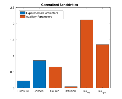
Figure 3: Bar graph of generalized parameter sensitivities.

From Figure 3, we can see that for this specific model problem it is most important to accurately measure the left and right boundary conditions. This makes sense intuitively, as the boundary conditions drive the fluid flow and the problem is advection dominated. We can also tell that in terms of data collection, it is more important to accurately measure concentration than pressure and that measuring the diffusion coefficient with a high degree of accuracy is relatively unimportant.

We consider the left boundary condition as an example and illustrate the interpretation of its generalized sensitivity index. Such principles of interpretation may be extended to any other generalized sensitivity indices but are omitted for conciseness. Figure 4 displays the true left boundary condition and the perturbation of the left boundary condition corresponding to the generalized sensitivity index (the argument of the maximization in (5). The perturbation plotted in Figure 4 is the unit norm perturbation that results in the maximum change in the inverse problem’s solution. Thus, the generalized sensitivity index $S_{5}=2.12$ indicates that this unit norm perturbation will result in a change of about 2.12 in the norm of the solution of the inverse problem. Scaling by the norm of the solution of the inverse problem gives an interpretation that the unit norm perturbation shown in Figure 4 results in approximately a $14\%$ change in the solution of the inverse problem. With this interpretation, a user may associate a level of uncertainty in the boundary condition and the resulting change in the estimated permeability field to determine if further calibration is needed.

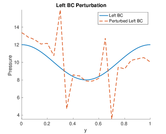
Figure 4: Perturbation of the left pressure Dirichlet boundary condition.

6.2 HDSA with Respect to Experimental Parameters

In this section, we turn to the pointwise hyper-differential sensitivities (4) to study the spatial and temporal dependence within the experimental parameters. Using the reconstructed log-permeability field, we compute the sensitivities of the solution with respect to both pressure and contaminant measurements at each sensor location, and for concentration, each time step. Figure 5 shows the spatial distribution of contaminant sensitivities (depicted by colored points using the right colorbar scale) at informative time snapshots, overlaid atop the tracer concentration field (depicted by a greyscale concentration map using the left colorbar scale). By overlaying these plots, we are able to study how the sensitivities relate to the tracer advection.

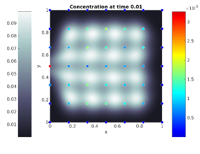
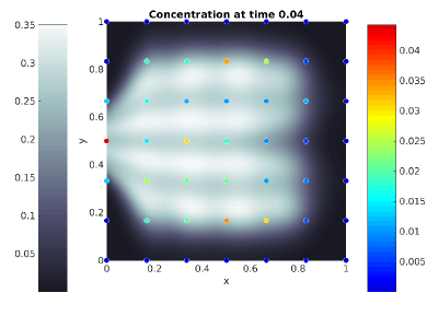
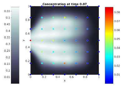
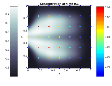
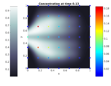
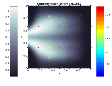
Figure 5: Concentration sensitivities at times 0.01, 0.04, 0.07, 0.10, 0.13, and 0.1567.

Note that both the sensitivity and concentration colorbar scales change in each plot, which is to allow the reader to visualize the results more clearly. We make the following observations about the concentration sensitivities. (1) As a general trend, the sensitivity of concentration increases in time. This is because the continuous source injection increases the amount of tracer in the domain as time progresses, making concentration sensors increasingly important. (2) We also see that as the mass of high tracer concentration (depicted by bright white in the color map) moves, sensors that observe this change in mass have increased importance while the mass moves toward or away from the sensor and then decrease in importance after the mass has moved passed. This phenomenon is particularly noticeable from the sensors in the high permeability channel at $y=0.5$. As the tracer mass moves from right to left at $y=0.5$ the sensor’s importance increases following the back edge of the mass, and then decreases after the mass moves past. (3) We also notice that the sensor on the left boundary at $y=.5$ is highly important early in time and the sensors at $(0.2,0.33)$ and $(0.2,0.66)$ are more important later in time. This is because the majority of the tracer is getting advected toward those sensors which are therefore observing a large amount of tracer flow.

To further study the concentration sensitivities, Figure 6 depicts the time evolution of each concentration sensitivity in an array of plots. Each plot describes the time evolution of a single contaminant sensitivity and they are spatially arranged to correspond to the sensor locations they depict (compare with Figure 1 for their spatial association).

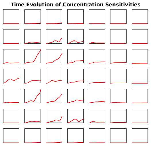
Figure 6: A spatial distribution of the time evolution of contaminant sensitivities. Each subplot has the same horizontal axis range depicting time from 0 to .16. Each vertical axis subplot has the same range depicting sensitivity from 0 to .2832

From Figure 6 we can see that some of the sensitivities decrease in importance over time, or have a range of time during which they decrease before they begin to increase again. Sensors for which the tracer permanently moves away experience a long-term decrease in importance. The decrease in sensitivity at a sensor location, followed by a subsequent increase is likely caused by the movement of tracer through the high permeability region at $y=0.5$. As the tracer empties out of this central region, the concentration changes from being a single mass to being two distinct masses, one in the upper portion and the other in the lower portion of the domain. This splitting of the concentration mass, when observed by a nearby sensor, likely causes a minor disturbance in the general trend of the sensitivity.

Because this problem is advection dominated, the movement of the tracer through the domain has a large impact on the interpretation of the pressure sensitivities as well. Figure 7 shows the spatial distribution of pressure sensitivities (depicted by colored points using the right colorbar scale) overlaid atop the pressure field (depicted by a greyscale pressure map using the left colorbar scale).

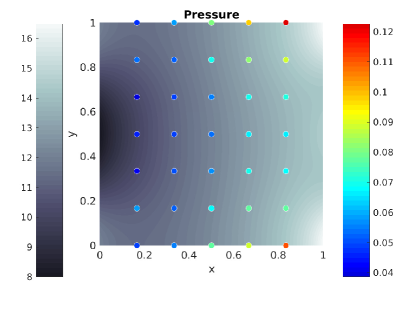
Figure 7: Pressure sensitivities

First, notice that the pressure sensitivities are larger than the concentration sensitivities at early time steps, but are eventually surpassed by the steadily increasing concentration sensitivities over time. Also observe that the sensors with highest pressure sensitivity, are in the upper right and lower right corners of the domain. Because the tracer moves from right to left, the majority of information about the tracer advection is found on the left side of the domain. The right side of the domain, and particularly the low permeability regions at the top and bottom, have a lack of tracer flow information. Thus, the inverse problem relies heavily on the pressure measurements in these regions to reconstruct the permeability field, which corresponds to the higher pressure sensitivities in this region.

6.3 HDSA with Respect to Auxiliary Parameters

In this section, we study the pointwise hyper-differential sensitivities with respect to auxiliary parameters: the source term and pressure Dirichlet boundary conditions. The diffusion coefficient is also an auxiliary parameter, however according to the generalized sensitivities it is relatively unimportant so we will not investigate it further.

We begin by analyzing the sensitivities with respect to the source term. Figure 8 depicts the sensitivities of the source at each injection well, next to a plot of the Darcy velocity field. The source uncertainty is discretized by taking a $3\times 3$ mesh locally around each well. This models our uncertainty in the rate and distribution of the injected tracer at each well due to hardware limitations, while the location of the injected tracer is known.

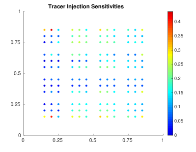
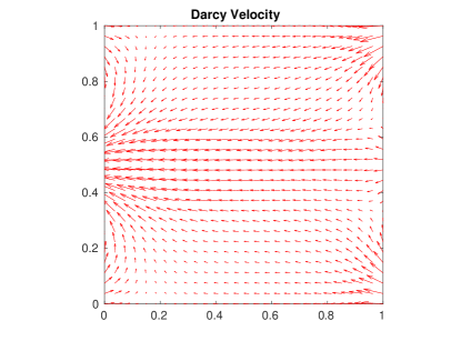
Figure 8: Left: Source sensitivities,  Right: Darcy Velocity Field

From Figure 8 we can see that the areas of high source sensitivity generally occur in regions with low Darcy velocity. This is likely because in these regions, the problem is diffusion dominated and the tracer is not advected away from the injection site very quickly. Thus, if the source injection is perturbed, the tracer will stay in that region and slowly diffuse, affecting concentration measurements in that area for may time steps. If a source injection is perturbed in a region of high Darcy velocity, the tracer will be pulled away and mix with the rest of the tracer moving through the domain. Thus for this problem, the source injections have highest sensitivity in regions that are diffusion dominated.

According to the generalized sensitivities, the boundary conditions have the largest relative impact of any uncertain parameter on the solution. To further understand the influence of the boundary conditions on the physical systems in the model, we consider the hyper-differential sensitivities of the boundary conditions. Figure 9 depicts the sensitivities of the solution with respect to the pressure Dirichlet boundary conditions, discretized by 21 equally spaced nodes on each boundary.

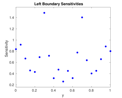
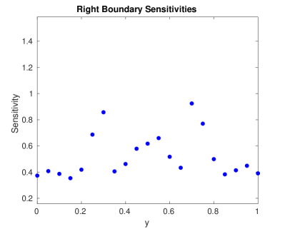
Figure 9: Pressure Dirichlet boundary condition sensitivities

From the boundary condition sensitivities in Figure 9 we can see that on both the left and right boundary, there is a heightened sensitivity around $y=0.3$ and $y=0.7$. This corresponds to the area between the high permeability region through the middle of the domain, and the low permeability regions above and below it. A perturbation of the boundary conditions near the low permeability region is going to have minimal effect because the low permeability region is going to keep the Darcy velocity small relative to the rest of the domain regardless. Similarly, a perturbation of the boundary conditions in the high permeability region is going to have little effect because the high permeability is going to keep the Darcy velocity relatively high in that area. A perturbation in the pressure boundary conditions will have maximal impact in the thin region between the high and low permeability regions. This perturbation can cause the region of moderate Darcy velocity to become a region of either high or low Darcy velocity relative to the other regions of the domain, significantly impacting the advection flow.

6.4 Discussion

It is evident from our analysis that the hyper-differential sensitivities can provide a wealth of information about how the solution of the inverse problem depends on the interactions within the governing physics systems. These observations are not readily apparent without the sensitivities, which emphasizes their usefulness in understanding the inverse problem. In particular, the sensitivities with respect to experimental parameters can be used to determine where and when to place expensive, high fidelity sensors in an experimental design, and where less accurate and more cost effective sensors can be uesd.

In addition to providing information about the underlying physics in a model, these observations allow experimenters to determine how to design experiments, by prioritizing the measurement and estimation of all complementary parameters considered. For this problem, the generalized sensitivities inform us that tracer concentration is more important to measure accurately than pressure, which informs the design of sensors and data collection techniques. We also learn that accurately estimating the pressure Dirichlet boundary conditions is highly important, while the diffusivity coefficient is relatively unimportant. This information informs the model specification and how these parameters should be estimated and considered in the model.

7 Conclusion

In this article, we have presented a mathematical framework for hyper-differential sensitivity analysis in the context of inverse problems constrained by multiphysics systems of partial differential equations. The mathematical formulation involves derivative based local sensitivity analysis of the solution of an inverse problem with respect to perturbations of parameters. This framework is general and can be applied to a wide variety of inverse problems. The usefulness of HDSA is most apparent in the context of complicated multiphysics systems with many uncertain parameters. By introducing sensitivity analysis with respect to experimental parameters and maturing the generalized hyper-differential sensitivity indices, we have enabled analysis of the relative importance of both auxiliary model parameters and experimental parameters, such as data sources. Studying hyper-differential sensitivities provides new insights into both understanding the underlying physical systems of a model, and designing experiments to solve inverse problems. In particular, comparing the relative importance of spatially and temporally distributed measurements with various sensor types provides unique insights that are difficult to attain using traditional experimental design methodologies. HDSA compliments experimental design by providing a systematic way to compare multiphysics parameters and data sources.

HDSA is an emerging technology and as such there are several important considerations to be studied in future work. One questions is “how robust are the sensitivities of experimental parameters to perturbations of design?” In practice, one may not be able to place a sensor exactly where a design indicates it should be. If a sensor’s location is perturbed within a local area, how will this affect the magnitude of the sensitivity, and that of its neighboring sensors? Ideally, perturbing the location of a sensor slightly will have a minimal impact on the sensitivity at that sensor and its neighbors, indicating that the hyper-differential sensitivities are robust to perturbations of the design, but this has yet to be rigorously verified.

Moreover, HDSA of inverse problems requires availability of measurement data. For the computational results in this paper, we assumed that we had some set of experimental data, but in many applications we would like to compute sensitivities a priori, before data is collected. In such cases, one could generate training data by applying the forward model to a sample of the inversion parameters drawn from a prior distribution, giving rise to a distribution of the sensitivities.

Appendix A Details for the model inverse problem (7)

First, we illustrate the computation of gradient and Hessian of $\hat{J}$. To facilitate this, we introduce the Lagrangian

$$\mathcal{L}(\boldsymbol{u},\boldsymbol{m},\boldsymbol{\lambda},\boldsymbol{\theta})=\hat{J}(\boldsymbol{m})+\boldsymbol{\lambda}^{\top}(\mathbf{{L}}(\boldsymbol{m})\boldsymbol{u}-\mathbf{{V}}\boldsymbol{\theta}),$$

where $\boldsymbol{\lambda}$ is a Lagrange multiplier (vector). To compute the gradient of $\hat{J}$, using the so called formal Lagrange approach, we consider the variations of $\mathcal{L}$ with respect to $\boldsymbol{\lambda}$, $\boldsymbol{u}$ and $\boldsymbol{m}$. Note that

$$\mathcal{L}_{\boldsymbol{\lambda}}(\boldsymbol{u},\boldsymbol{m},\boldsymbol{\lambda},\boldsymbol{\theta})=\mathbf{{L}}(\boldsymbol{m})\boldsymbol{u}-\mathbf{{V}}\boldsymbol{\theta}\quad\text{and}\quad\mathcal{L}_{\boldsymbol{u}}(\boldsymbol{u},\boldsymbol{m},\boldsymbol{\lambda},\boldsymbol{\theta})=\frac{\partial\hat{J}}{\partial\boldsymbol{u}}+\boldsymbol{\lambda}^{\top}\mathbf{{L}}(\boldsymbol{m}).$$

Setting these variations equal to 0 results in the state and the adjoint equations:

$$\mathbf{{L}}(\boldsymbol{m})\boldsymbol{u}=\mathbf{{V}}\boldsymbol{\theta}\quad\text{and}\quad\mathbf{{L}}(\boldsymbol{m})^{\top}\boldsymbol{\lambda}=-\mathbf{{Q}}^{\top}\mathbf{{W}}(\mathbf{{Q}}\boldsymbol{u}-\boldsymbol{y}).$$

Then, the gradient $g(\boldsymbol{m})$ of $\hat{J}$ satisfies, $g(\boldsymbol{m})^{T}=\mathcal{L}_{\boldsymbol{m}}(\boldsymbol{u},\boldsymbol{m},\boldsymbol{\lambda},\boldsymbol{\theta})=\frac{\partial\hat{J}}{\partial\boldsymbol{m}}+\boldsymbol{\lambda}^{\top}\frac{\partial\mathbf{{A}}}{\partial\boldsymbol{m}}\boldsymbol{u}$; therefore,

$$g(\boldsymbol{m})=\alpha\mathbf{{R}}\boldsymbol{m}+\mathbf{{C}}^{\top}\boldsymbol{\lambda}\quad\text{with}\quad\mathbf{{C}}=\frac{\partial}{\partial\boldsymbol{m}}\big{(}\mathbf{{L}}(\boldsymbol{m})\boldsymbol{u}\big{)}.$$

To compute the action of the Hessian $\mathbf{{H}}(\boldsymbol{m})$ of $\hat{J}$ (at $\boldsymbol{m}$) on a vector $\widehat{}\boldsymbol{m}$, we differentiate through the directional derivative $\langle g(\boldsymbol{m}),\widehat{\boldsymbol{m}}\rangle$. This is faciliated by introducing the “meta-Lagrangian”:

$$\mathcal{L}^{H}(\boldsymbol{u},\boldsymbol{m},\boldsymbol{\lambda},\boldsymbol{\theta},\widehat{\boldsymbol{u}},\widehat{\boldsymbol{\lambda}};\widehat{\boldsymbol{m}})=\widehat{\boldsymbol{m}}^{\top}\big{[}\mathbf{{C}}^{\top}\boldsymbol{\lambda}+\alpha\mathbf{{R}}\boldsymbol{m}\big{]}+\widehat{\boldsymbol{\lambda}}^{\top}\big{[}\mathbf{{L}}(\boldsymbol{m})\boldsymbol{u}-\mathbf{{V}}\boldsymbol{\theta}\big{]}+\\ \widehat{\boldsymbol{u}}^{\top}\big{[}\mathbf{{L}}(\boldsymbol{m})^{\top}\boldsymbol{\lambda}+\mathbf{{Q}}^{\top}\mathbf{{W}}(\mathbf{{Q}}\boldsymbol{u}-\boldsymbol{y})\big{]}.$$

The Lagrange multipliers $\widehat{\boldsymbol{u}}$ and $\widehat{\boldsymbol{\lambda}}$ are refered to as the incremental state and adjoint variables; see e.g., [36]. Letting the variations of $\mathcal{L}^{H}$ with respect to $\widehat{\boldsymbol{\lambda}}$ and $\widehat{\boldsymbol{u}}$ vanish gives

$$\mathbf{{L}}(\boldsymbol{m})\widehat{\boldsymbol{u}} =-\mathbf{{C}}\widehat{\boldsymbol{m}},\quad$$ (incremental state equation) (9)

$$\mathbf{{L}}(\boldsymbol{m})^{\top}\widehat{\boldsymbol{\lambda}} =-\mathcal{L}_{\boldsymbol{u}\boldsymbol{m}}\widehat{\boldsymbol{m}}-\mathcal{L}_{\boldsymbol{u}\boldsymbol{u}}\widehat{\boldsymbol{u}}.\quad$$ (incremental adjoint equation) (10)

The Hessian apply is then given by, $\left[\mathbf{{H}}(\boldsymbol{m})\widehat{\boldsymbol{m}}\right]^{\top}=\mathcal{L}_{\boldsymbol{m}}^{H}\widehat{}\boldsymbol{m}$, resulting in

$$\mathbf{{H}}(\boldsymbol{m})\widehat{\boldsymbol{m}}=\mathcal{L}_{\boldsymbol{m}\boldsymbol{m}}\widehat{\boldsymbol{m}}+\mathcal{L}_{\boldsymbol{m}\boldsymbol{u}}\widehat{\boldsymbol{u}}+\mathbf{{C}}^{\top}\widehat{\boldsymbol{\lambda}}.$$ (11)

Note that in the above equations

$$\mathcal{L}_{\boldsymbol{u}\boldsymbol{u}}=\mathbf{{Q}}^{\top}\mathbf{{W}}\mathbf{{Q}},\quad\mathcal{L}_{\boldsymbol{m}\boldsymbol{m}}=\alpha\mathbf{{R}}+\frac{\partial}{\partial\boldsymbol{m}}(\mathbf{{C}}^{T}\boldsymbol{\lambda}),\quad\text{and}\quad\mathcal{L}_{\boldsymbol{m}\boldsymbol{u}}=\mathcal{L}_{\boldsymbol{u}\boldsymbol{m}}^{\top}=\frac{\partial}{\partial\boldsymbol{m}}(\mathbf{{L}}(\boldsymbol{m})^{T}\boldsymbol{\lambda})$$

We summarize the compuation of $\mathbf{{H}}(\boldsymbol{m})\widehat{\boldsymbol{m}}$ in Algorithm 1.

Algorithm 1 Computation of $\mathbf{{H}}(\boldsymbol{m})\widehat{\boldsymbol{m}}$ for a given $\widehat{\boldsymbol{m}}$.

  solve the incremental state equation (9) for $\widehat{\boldsymbol{u}}$

  Solve the incremental adjoint equation (10) for $\widehat{\boldsymbol{\lambda}}$

  Evaluate $\mathbf{{H}}(\boldsymbol{m})\widehat{\boldsymbol{m}}$ accordng to (11).

Note that the cost associates with Algorithm 1 is two (linear) PDE solves. Also, by replacing the expressions for the incremental state and adjoint variables in the expression for the Hessian apply, we can write the (reduced) Hessian as:

$$\mathbf{{H}}=\mathbf{{C}}^{\top}\mathbf{{L}}(\boldsymbol{m})^{-\top}\mathcal{L}_{\boldsymbol{u}\boldsymbol{u}}\mathbf{{L}}(\boldsymbol{m})^{-1}\mathbf{{C}}+\mathcal{L}_{\boldsymbol{m}\boldsymbol{m}}-\mathcal{L}_{\boldsymbol{m}\boldsymbol{u}}\mathbf{{L}}(\boldsymbol{m})^{-1}\mathbf{{C}}-\mathbf{{C}}^{\top}\mathbf{{L}}(\boldsymbol{m})^{-\top}\mathcal{L}_{\boldsymbol{u}\boldsymbol{m}}.$$

Letting $\mathbf{{B}}$ be the (discretized) Fréchet derivative of the gradient with respect to $\boldsymbol{\theta}$,

$$\mathbf{{B}}=g_{\boldsymbol{\theta}}(\boldsymbol{m})=-\mathbf{{C}}^{\top}\mathbf{{L}}(\boldsymbol{m})^{-\top}\mathbf{{Q}}^{\top}\mathbf{{W}}\mathbf{{Q}}\mathbf{{L}}(\boldsymbol{m})^{-1}\mathbf{{V}}+\mathcal{L}_{\boldsymbol{m}\boldsymbol{u}}\mathbf{{L}}(\boldsymbol{m})^{-1}\mathbf{{V}}.$$

This is the discretized version of the operator $\mathcal{B}$ in (3).

Bibliography

Bibliography

- [1] Joseph Hart, Bart van Bloemen Waanders, and Roland Herzog. Hyper-differential sensitivity analysis of uncertain parameters in PDE-constrained optimization. To appear in the International Journal for Uncertainty Quantification, 2020. https://arxiv.org/abs/1909.07336.
- [2] Kerstin Brandes and Roland Griesse. Quantitative stability analysis of optimal solutions in PDE-constrained optimization. Journal of Computational and Applied Mathematics, 2006.
- [3] C. Büskens and R. Griesse. Parametric sensitivity analysis of perturbed PDE optimal control problems with state and control constraints. Journal of Optimization Theory and Applications, 131(1):17–35, 2006.
- [4] Roland Griesse. Parametric sensitivity analysis in optimal control of a reaction-diffusion system – part II: practical methods and examples. Optimization Methods and Software, 19(2):217–242, 2004.
- [5] Roland Griesse. Parametric sensitivity analysis in optimal control of a reaction diffusion system. I. solution differentiability. Numerical Functional Analysis and Optimization, 25(1-2):93–117, 2004.
- [6] Roland Griesse. Stability and sensitivity analysis in optimal control of partial differential equations. Habilitation Thesis, Faculty of Natural Sciences, Karl-Franzens University, 2007.
- [7] Roland Griesse and Boris Vexler. Numerical sensitivity analysis for the quantity of interest in PDE-Constrained optimization. SIAM Journal on Scientific Computing, 29(1):22–48, 2007.
- [8] R. Griesse and S. Volkwein. Parametric sensitivity analysis for optimal boundary control of a 3D reaction-difusion system. In G. Di Pillo and M. Roma, editors, Nonconvex Optimization and its Applications, volume 83. Springer, Berlin, 2006.
- [9] Roland Griesse and Andrea Walther. Parametric sensitivities for optimal control problems using automatic differentiation. Optimal Control Applications and Methods, 24:297–314, 2003.
- [10] A. Pázman. Foundations of Optimum Experimental Designs. D. Reidel Publishing Co., 1986.
- [11] A. C. Atkinson and A. N. Donev. Optimum Experimental Designs. Oxford, 1992.
- [12] Dariusz Uciński. Optimal Measurement Methods for Distributed Parameter System Identification. CRC Press, Boca Raton, 2005.
- [13] Karina Koval, Alen Alexanderian, and Georg Stadler. Optimal experimental design under irreducible uncertainty for inverse problems governed by PDEs. Submitted, 2019. https://arxiv.org/abs/1912.08915.
- [14] A M. Stuart. Inverse problems: A Bayesian perspective. Acta Numerica, 19:451–559, 05 2010.
- [15] Volkan Akçelik, George Biros, Omar Ghattas, Judith Hill, David Keyes, and Bart van Bloemen Waanders. Parallel Processing for Scientific Computing, chapter Parallel Algorithms for PDE-Constrained Optimization. SIAM, 2006.
- [16] Tan Bui-Thanh. A gentle tutorial on statistical inversion using the Bayesian paradigm. Technical report, The University of Texas at Austin, 2012.
- [17] Masoumeh Dashti and Andrew M. Stuart. The Bayesian approach to inverse problems. Handbook of Uncertainty Quantification, 2017.
- [18] H.W. Engl, M. Hanke, and A. Neubauer. Regularization of Inverse Problems. Kluwer Academic Publishers, 1996.
- [19] Kazufumi Ito and Bangti Jin. Inverse problems: Tikhonov theory and algorithms. World Scientific, 2015.
- [20] Jari Kaipio and Erkki Somersalo. Statistical and Computational Inverse Problems. Springer, 2005.
- [21] Albert Tarantola. Inverse Problem Theory and Methods for Model Parameter Estimation. Society for Industrial and Applied Mathematics, 2005.
- [22] Curtis Vogel. Computational Methods for Inverse Problems. Society for Industrial and Applied Mathematics, 2002.
- [23] Irene Bauer, Hans G. Bock, Stefan Körkel, and Johannes P. Schlöder. Numerical methods for optimum experimental design in DAE systems. Journal of Computational and Applied Mathematics, 120(1-2):1–25, 2000. SQP-based direct discretization methods for practical optimal control problems.
- [24] Stefan Körkel, Ekaterina Kostina, Hans G. Bock, and Johannes P. Schlöder. Numerical methods for optimal control problems in design of robust optimal experiments for nonlinear dynamic processes. Optimization Methods & Software, 19(3-4):327–338, 2004. The First International Conference on Optimization Methods and Software. Part II.
- [25] Eldad Haber, Lior Horesh, and Luis Tenorio. Numerical methods for experimental design of large-scale linear ill-posed inverse problems. Inverse Problems, 24(055012):125–137, 2008.
- [26] Hans Georg Bock, Stefan Körkel, and Johannes P. Schlöder. Parameter estimation and optimum experimental design for differential equation models. In Hans Georg Bock, Thomas Carraro, Willi Jäger, Stefan Körkel, Rolf Rannacher, and Johannes P. Schlöder, editors, Model Based Parameter Estimation, volume 4 of Contributions in Mathematical and Computational Sciences, pages 1–30. Springer Berlin Heidelberg, 2013.
- [27] Xun Huan and Youssef M. Marzouk. Simulation-based optimal Bayesian experimental design for nonlinear systems. Journal of Computational Physics, 232(1):288–317, 2013.
- [28] Quan Long, Marco Scavino, Raúl Tempone, and Suojin Wang. Fast estimation of expected information gains for Bayesian experimental designs based on Laplace approximations. Computer Methods in Applied Mechanics and Engineering, 259:24–39, 2013.
- [29] Quan Long, Mohammad Motamed, and Raúl Tempone. Fast Bayesian optimal experimental design for seismic source inversion. Computer Methods in Applied Mechanics and Engineering, 291:123–145, 2015.
- [30] Eldad Haber, Lior Horesh, and Luis Tenorio. Numerical methods for the design of large-scale nonlinear discrete ill-posed inverse problems. Inverse Problems, 26(2):025002, 2010.
- [31] Lior Horesh, Eldad Haber, and Luis Tenorio. Optimal Experimental Design for the Large-Scale Nonlinear Ill-Posed Problem of Impedance Imaging, pages 273–290. Wiley, 2010.
- [32] Alen Alexanderian, Noemi Petra, Georg Stadler, and Omar Ghattas. A-optimal design of experiments for infinite-dimensional Bayesian linear inverse problems with regularized -sparsification. SIAM Journal on Scientific Computing, 36(5):A2122–A2148, 2014.
- [33] Alen Alexanderian, Noemi Petra, Georg Stadler, and Omar Ghattas. A fast and scalable method for a-optimal design of experiments for infinite-dimensional Bayesian nonlinear inverse problems. SIAM J. Scientific Computing, 38(1), 2016.
- [34] Alen Alexanderian and Arvind K Saibaba. Efficient D-optimal design of experiments for infinite-dimensional Bayesian linear inverse problems. SIAM Journal on Scientific Computing, 40(5):A2956–A2985, 2018.
- [35] Antonio Ambrosetti and Giovanni Prodi. A Primer of Nonlinear Analysis. Cambridge University Press, 1995.
- [36] N. Petra and G. Stadler. Model variational inverse problems governed by partial differential equations. Technical report, The University of Texas at Austin, 2011.