Differential Privacy at Risk: Bridging Randomness and Privacy Budget

Abstract

The calibration of noise for a privacy-preserving mechanism depends on the sensitivity of the query and the prescribed privacy level. A data steward must make the non-trivial choice of a privacy level that balances the requirements of users and the monetary constraints of the business entity.
We analyse roles of the sources of randomness, namely the explicit randomness induced by the noise distribution and the implicit randomness induced by the data-generation distribution, that are involved in the design of a privacy-preserving mechanism. The finer analysis enables us to provide stronger privacy guarantees with quantifiable risks. Thus, we propose privacy at risk that is a probabilistic calibration of privacy-preserving mechanisms. We provide a composition theorem that leverages privacy at risk. We instantiate the probabilistic calibration for the Laplace mechanism by providing analytical results.
We also propose a cost model that bridges the gap between the privacy level and the compensation budget estimated by a GDPR compliant business entity. The convexity of the proposed cost model leads to a unique fine-tuning of privacy level that minimises the compensation budget. We show its effectiveness by illustrating a realistic scenario that avoids overestimation of the compensation budget by using privacy at risk for the Laplace mechanism. We quantitatively show that composition using the cost optimal privacy at risk provides stronger privacy guarantee than the classical advanced composition.

1 Introduction

Dwork et al. quantify the privacy level $\varepsilon$ in $\varepsilon$-differential privacy as an upper bound on the worst-case privacy loss incurred by a privacy-preserving mechanism. Generally, a privacy-preserving mechanism perturbs the results by adding the calibrated amount of random noise to them. The calibration of noise depends on the sensitivity of the query and the specified privacy level. In a real-world setting, a data steward must specify a privacy level that balances the requirements of the users and monetary constraints of the business entity. Garfinkel et al. report the issues in deploying differential privacy as the privacy definition by the US census bureau. They highlight the lack of analytical methods to choose the privacy level. They also report empirical studies that show the loss in utility due to the application of privacy-preserving mechanisms.

We address the dilemma of a data steward in two ways. Firstly, we propose a probabilistic quantification of privacy levels. Probabilistic quantification of privacy levels provides a data steward a way to take quantified risks under the desired utility of the data. We refer to the probabilistic quantification as privacy at risk. We also derive a composition theorem that leverages privacy at risk. Secondly, we propose a cost model that links the privacy level to a monetary budget. This cost model helps the data steward to choose the privacy level constrained on the estimated budget and vice versa. Convexity of the proposed cost model ensures the existence of a unique privacy at risk that would minimise the budget. We show that the composition with an optimal privacy at risk provides stronger privacy guarantees than the traditional advanced composition (Dwork et al., 2014). In the end, we illustrate a realistic scenario that exemplifies how the data steward can avoid overestimation of the budget by using the proposed cost model by using privacy at risk.

The probabilistic quantification of privacy levels depends on two sources of randomness: the explicit randomness induced by the noise distribution and the implicit randomness induced by the data-generation distribution. Often, these two sources are coupled with each other. We require analytical forms of both sources of randomness as well as an analytical representation of the query to derive a privacy guarantee. Computing the probabilistic quantification is generally a challenging task. Although we find multiple probabilistic privacy definitions in the literature (Machanavajjhala et al., 2008; Hall et al., 2012), we are missing analytical quantification bridging the randomness and privacy level of a privacy-preserving mechanism. To the best of our knowledge, we are the first to analytically derive such a probabilistic quantification, namely privacy at risk, for the widely used Laplace mechanism (Dwork et al., 2006b). We also derive a composition theorem with privacy at risk. It is a special case of the advanced composition theorem (Dwork et al., 2014) that deals with a sequential and adaptive use of privacy-preserving mechanisms. We work on a simpler model independent evaluations used in the basic composition theorem (Dwork et al., 2014).

The privacy level proposed by the differential privacy framework is too abstract a quantity to be integrated in a business setting. We propose a cost model that maps the privacy level to a monetary budget. The corresponding cost model for the probabilistic quantification of privacy levels is a convex function of the privacy level. Hence, it leads to a unique probabilistic privacy level that minimises the cost. We illustrate a realistic scenario in a GDPR compliant business entity that needs an estimation of the compensation budget that it needs to pay to stakeholders in the unfortunate event of a personal data breach. The illustration shows that the use of probabilistic privacy levels avoids overestimation of the compensation budget without sacrificing utility.

In this work, we comparatively evaluate the privacy guarantees using privacy at risk of using Laplace mechanism. We quantitatively compare the composition under the optimal privacy at risk, which is estimated using the cost model, with traditional composition mechanisms - the basic composition and advanced mechanism (Dwork et al., 2014). We observe that it gives stronger privacy guarantees than the ones by the advanced composition without sacrificing on the utility of the mechanism.

In conclusion, benefits of the probabilistic quantification i.e. the privacy at risk are twofold. It not only quantifies the privacy level for a given privacy-preserving mechanism but also facilitates decision-making in problems that focus on the privacy-utility trade-off and the compensation budget minimisation.

2 Background

We consider a universe of datasets $\mathcal{D}$. We explicitly mention when we consider that the datasets are sampled from a data-generation distribution $\mathcal{G}$ with support $\mathcal{D}$. Two datasets of equal cardinality $x$ and $y$ are said to be neighbouring datasets if they differ in one data point. A pair of neighbouring datasets is denoted by $x\sim y$. In this work, we focus on a specific class of queries called numeric queries. A numeric query $f$ is a function that maps a dataset into a real-valued vector, i.e. $f:\mathcal{D}\rightarrow\mathbb{R}^{k}$. For instance, a sum query returns the sum of the values in a dataset.

In order to achieve a privacy guarantee, a privacy-preserving mechanism, or mechanism in short, is a randomised algorithm, that adds noise to the query from a given family of distributions. Thus, a privacy-preserving mechanism of a given family, $\mathcal{M}(f,\Theta)$, for the query $f$ and the set of parameters $\Theta$ of the given noise distribution, is a function that maps a dataset into a real vector, i.e. $\mathcal{M}(f,\Theta):\mathcal{D}\rightarrow\mathbb{R}^{k}$. We denote a privacy-preserving mechanism as $\mathcal{M}$, when the query and the parameters are clear from the context.

Definition 1

[Differential Privacy (Dwork et al., 2014).] A privacy-preserving mechanism $\mathcal{M}$, equipped with a query $f$ and with parameters $\Theta$, is $(\varepsilon,\delta)$-differentially private if for all $Z\subseteq\textrm{Range}(\mathcal{M})$ and $x,y\in\mathcal{D}$ such that $x\sim y$:

$$\mathbb{P}(\mathcal{M}(f,\Theta)(x)\in Z)\leq\text{e}^{\varepsilon}\mathbb{P}(\mathcal{M}(f,\Theta)(y)\in Z)+\delta$$

$(\varepsilon,0)$-differentially private mechanism is ubiquitously called as $\varepsilon$-differentially private.

A privacy-preserving mechanism provides perfect privacy if it yields indistinguishable outputs for all neighbouring input datasets. The privacy level $\varepsilon$ quantifies the privacy guarantee provided by $\varepsilon$-differential privacy. For a given query, the smaller the value of the $\varepsilon$, the qualitatively higher is the privacy. A randomised algorithm that is $\varepsilon$-differentially private is also $\varepsilon^{\prime}$-differential private for any $\varepsilon^{\prime}>\varepsilon$.

In order to satisfy $\varepsilon$-differential privacy, the parameters of a privacy-preserving mechanism requires a calculated calibration. The amount of noise required to achieve a specified privacy level depends on the query. If the output of the query does not change drastically for two neighbouring datasets, then small amount of noise is required to achieve a given privacy level. The measure of such fluctuations is called the sensitivity of the query. The parameters of a privacy-preserving mechanism are calibrated using the sensitivity of the query that quantifies the smoothness of a numeric query.

Definition 2

[Sensitivity.] The sensitivity of a query $f:\mathcal{D}\rightarrow\mathbb{R}^{k}$ is defined as

$$\Delta_{f}\triangleq\max_{\begin{subarray}{c}x,y\in\mathcal{D}\\ x\sim y\end{subarray}}~{}\lVert f(x)-f(y)\rVert_{1}.$$

The Laplace mechanism is a privacy-preserving mechanism that adds scaled noise sampled from a calibrated Laplace distribution to the numeric query.

Definition 3

[(Papoulis and Pillai, 2002)] The Laplace distribution with mean zero and scale $b>0$ is a probability distribution with probability density function

$$\mathrm{Lap}(b)\triangleq\frac{1}{2b}\exp{(-\frac{|x|}{b})},$$

where $x\in\mathbb{R}$. We write $\mathrm{Lap}(b)$ to denote a random variable $X\sim\mathrm{Lap}(b)$

Definition 4

[Laplace Mechanism (Dwork et al., 2006b).] Given any function $f:\mathcal{D}\rightarrow\mathbb{R}^{k}$ and any $x\in\mathcal{D}$, the Laplace Mechanism is defined as

$$\mathcal{L}^{\Delta_{f}}_{\varepsilon}(x)\triangleq\mathcal{M}\left(f,~{}\frac{\Delta_{f}}{\varepsilon}\right)(x)=f(x)+(L_{1},...,L_{k}),$$

where $L_{i}$ is drawn from $\mathrm{Lap}\left(\frac{\Delta_{f}}{\varepsilon}\right)$ and added to the $i^{\mathrm{th}}$ component of $f(x)$.

Theorem 5

(Dwork et al., 2006b) The Laplace mechanism, $\mathcal{L}^{\Delta_{f}}_{\varepsilon_{0}}$, is $\varepsilon_{0}$-differentially private.

3 Privacy at Risk: A Probabilistic Quantification of Randomness

The parameters of a privacy-preserving mechanism are calibrated using the privacy level and the sensitivity of the query. A data steward needs to choose appropriate privacy level for practical implementation. Lee and Clifton show that the choice of an actual privacy level by a data steward in regard to her business requirements is a non-trivial task. Recall that the privacy level in the definition of differential privacy corresponds to the worst case privacy loss. Business users are however used to taking and managing risks, if the risks can be quantified. For instance, Jorion defines Value at Risk that is used by risk analysts to quantify the loss in investments for a given portfolio and an acceptable confidence bound. Motivated by the formulation of Value at Risk, we propose to use the use of probabilistic privacy level. It provides us a finer tuning of an $\varepsilon_{0}$-differentially private privacy-preserving mechanism for a specified risk $\gamma$.

Definition 6

[Privacy at Risk.] For a given data generating distribution $\mathcal{G}$, a privacy-preserving mechanism $\mathcal{M}$, equipped with a query $f$ and with parameters $\Theta$, satisfies $\varepsilon$-differential privacy with a privacy at risk $0\leq\gamma\leq 1$, if for all $Z\subseteq\textrm{Range}(\mathcal{M})$ and $x,y$ sampled from $\mathcal{G}$ such that $x\sim y$:

$$\mathbb{P}\left[\left|\ln{\frac{\mathbb{P}(\mathcal{M}(f,\Theta)(x)\in Z)}{\mathbb{P}(\mathcal{M}(f,\Theta)(y)\in Z)}}\right|>\varepsilon\right]\leq\gamma,$$ (1)

where the outer probability is calculated with respect to the probability space $\mathrm{Range}(\mathcal{M}\circ\mathcal{G})$ obtained by applying the privacy-preserving mechanism $\mathcal{M}$ on the data-generation distribution $\mathcal{G}$.

If a privacy-preserving mechanism is $\varepsilon_{0}$-differentially private for a given query $f$ and parameters $\Theta$, for any privacy level $\varepsilon\geq\varepsilon_{0}$, privacy at risk is $0$. Our interest is to quantify the risk $\gamma$ with which $\varepsilon_{0}$-differentially private privacy-preserving mechanism also satisfies a stronger $\varepsilon$-differential privacy, i.e. $\varepsilon<\varepsilon_{0}$.

Unifying Probabilistic and Random Differential Privacy. As a natural consequence, Equation 1 unifies the notions of probabilistic differential privacy and random differential privacy by accounting for both sources of randomness in a privacy-preserving mechanism. Machanavajjhala et al. define probabilistic differential privacy that incorporates the explicit randomness of the noise distribution of the privacy-preserving mechanism whereas Hall et al. define random differential privacy that incorporates the implicit randomness of the data-generation distribution. In probabilistic differential privacy, the outer probability is computed over the sample space of $\mathrm{Range}(\mathcal{M})$ and all datasets are equally probable.

3.1 Composition theorem

Application of $\varepsilon$-differential privacy to many real-world problem suffers from the degradation of privacy guarantee, i.e. privacy level, over the composition. The basic composition theorem (Dwork et al., 2014) dictates that the privacy guarantee degrades linear in the number of evaluations of the mechanism. Advanced composition theorem (Dwork et al., 2014) provides a finer analysis of the privacy loss over multiple evaluations and provides a square root dependence on the the number of evaluations. In this section, we provide the composition theorem for privacy at risk.

Definition 7

[Privacy loss random variable.] For a privacy-preserving mechanism $\mathcal{M}:\mathcal{D}\rightarrow R$ and two neighbouring datasets $x,y\in\mathcal{D}$, the privacy loss random variable $\mathcal{C}$ takes a value $r\in R$

$$\mathcal{C}\triangleq\ln{\frac{\mathbb{P}(\mathcal{M}(x))}{\mathbb{P}(\mathcal{M}(y))}}$$

Lemma 8

If a privacy-preserving mechanism $\mathcal{M}$ satisfies $\varepsilon_{0}$ differential privacy, then

$$\mathbb{P}[|\mathcal{C}|\leq\varepsilon_{0}]=1$$

Theorem 9

For all $\varepsilon_{0},\varepsilon,\gamma,\delta>0$, the class of $\varepsilon_{0}$-differentially private mechanisms, which satisfy $(\varepsilon,\gamma)$-privacy at risk, are $(\varepsilon^{\prime},\delta)$-differential privacy under $n$-fold composition where

$$\varepsilon^{\prime}=\varepsilon_{0}\sqrt{2n\ln{\frac{1}{\delta}}}+n\mu$$

where, $\mu=[\gamma\varepsilon(e^{\varepsilon}-1)+(1-\gamma)\varepsilon_{0}(e^{\varepsilon_{0}}-1)]$

Proof  Let, $\mathcal{M}^{1...n}:\mathcal{D}\rightarrow R^{1}\times R^{2}\times...\times R^{n}$ denote the $n$-fold composition of privacy-preserving mechanisms $\{\mathcal{M}^{i}:\mathcal{D}\rightarrow R^{i}\}_{i=1}^{n}$. Each $\varepsilon_{0}$-differentially private $\mathcal{M}^{i}$ also satisfies $(\varepsilon,\gamma)$-privacy at risk for some $\varepsilon\leq\varepsilon_{0}$ and appropriately computer $\gamma$. Consider any two neighbouring datasets $x,y\in\mathcal{D}$. Let,

$$B=\{(r_{1},...,r_{n})|\bigwedge_{i=1}^{n}\frac{\mathbb{P}(\mathcal{M}^{i}(x)=r_{i})}{\mathbb{P}(\mathcal{M}^{i}(y)=r_{i})}>\text{e}^{\varepsilon}\}$$

Using the technique in (Dwork et al., 2014, Theorem 3.20), it suffices to show that $\mathbb{P}(\mathcal{M}^{1...n}(x)\in B)\leq\delta$.

Consider,

$$\ln{\frac{\mathbb{P}(\mathcal{M}^{1...n}(x)=(r_{1},...,r_{n}))}{\mathbb{P}(\mathcal{M}^{1...n}(y)=(r_{1},...,r_{n}))}}$$

$$= \ln{\prod_{i=1}^{n}}\frac{\mathbb{P}(\mathcal{M}^{i}(x)=r_{i})}{\mathbb{P}(\mathcal{M}^{i}(y)=r_{i})}$$

$$= \sum_{i=1}^{n}\ln{\frac{\mathbb{P}(\mathcal{M}^{i}(x)=r_{i})}{\mathbb{P}(\mathcal{M}^{i}(y)=r_{i})}}~{}=~{}\sum_{i=1}^{n}\mathcal{C}^{i}$$ (2)

where $\mathcal{C}^{i}$ in the last line denotes privacy loss random variable related $\mathcal{M}^{i}$.

Consider, an $\varepsilon$-differentially private mechanism $\mathcal{M}_{\varepsilon}$ and $\varepsilon_{0}$-differentially private mechanism $\mathcal{M}_{\varepsilon_{0}}$. Let $\mathcal{M}_{\varepsilon_{0}}$ satisfy $(\varepsilon,\gamma)$-privacy at risk for $\varepsilon\leq\varepsilon_{0}$ and appropriately computed $\gamma$. Each $\mathcal{M}^{i}$ can be simulated as the mechanism $\mathcal{M}_{\varepsilon}$ with probability $\gamma$ and the mechanism $\mathcal{M}_{\varepsilon_{0}}$ otherwise. Therefore, privacy loss random variable for each mechanism $\mathcal{M}^{i}$ can be written as

$$\mathcal{C}^{i}=\gamma\mathcal{C}_{\varepsilon}^{i}+(1-\gamma)\mathcal{C}_{\varepsilon_{0}}^{i}$$

where, $\mathcal{C}_{\varepsilon}^{i}$ denotes the privacy loss random variable associated with the mechanism $\mathcal{M}_{\varepsilon}$ and $\mathcal{C}_{\varepsilon_{0}}^{i}$ denotes the privacy loss random variable associated with the mechanism $\mathcal{M}_{\varepsilon_{0}}$. Using (Dwork et al., 2014, Lemma $3.18$), we can bound the mean of every privacy loss random variable as,

$$\mu\triangleq\mathbb{E}[\mathcal{C}^{i}]\leq[\gamma\varepsilon(e^{\varepsilon}-1)+(1-\gamma)\varepsilon_{0}(e^{\varepsilon_{0}}-1)]$$

We have a collection of $n$ independent privacy random variables $\mathcal{C}^{i}$s such that $\mathbb{P}\left[|\mathcal{C}^{i}|\leq\varepsilon_{0}\right]=1$. Using Hoeffding’s bound (Hoeffding, 1994) on the sample mean for any $\beta>0$,

$$\mathbb{P}\left[\frac{1}{n}\sum_{i}C^{i}\geq\mathbb{E}[\mathcal{C}^{i}]+\beta\right]\leq\exp{\left(-\frac{n\beta^{2}}{2\varepsilon_{0}^{2}}\right)}$$

Rearranging the inequality by renaming the upper bound on the probability as $\delta$, we get,

$$\mathbb{P}\left[\sum_{i}C^{i}\geq n\mu+\varepsilon_{0}\sqrt{2n\ln{\frac{1}{\delta}}}\right]\leq\delta$$

 

Theorem 9 is an analogue, in the privacy at risk setting, of the advanced composition of differential privacy (Dwork et al., 2014, Theorem 3.20) under a constraint of independent evaluations. Note that, if one takes $\gamma=0$, then we obtain the exact same formula as in (Dwork et al., 2014, Theorem 3.20). It provides a sanity check for the consistency of composition using privacy at risk.

In fact, if we consider both sources of randomness, the expected value of loss function must be computed by using the law of total expectation.

$$\mathbb{E}[\mathcal{C}]=\mathbb{E}_{x,y\sim\mathcal{G}}[\mathbb{E}[\mathcal{C}]|x,y]$$

Therefore, the exact computation of privacy guarantees after the composition requires access to the data-generation distribution. We assume a uniform data-generation distribution while proving Theorem 9. We can obtain better and finer privacy guarantees accounting for data-generation distribution, which we keep as a future work.

3.2 Convexity and Post-processing

Since privacy at risk provides a probabilistic privacy guarantee for an $\varepsilon_{0}$-differentially private mechanism, it does not alter the basic properties of differential privacy - convexity and post-processing. We now show that privacy at risk equally adheres to both of these properties.

Lemma 10 (Convexity)

For a given $\varepsilon_{0}$-differentially private privacy-preserving mechanism, privacy at risk satisfies convexity property.

Proof  Let $\mathcal{M}$ be a mechanism that satisfies $\varepsilon_{0}$-differential privacy. By the definition of the privacy at risk, it also satisfies $(\varepsilon_{1},\gamma_{1})$-privacy at risk as well as $(\varepsilon_{2},\gamma_{2})$-privacy at risk for some $\varepsilon_{1},\varepsilon_{2}\leq\varepsilon_{0}$ and appropriately computed values of $\gamma_{1}$ and $\gamma_{2}$. Let $\mathcal{M}^{1}$ and $\mathcal{M}^{2}$ denote the hypothetical mechanisms that satisfy $(\varepsilon_{1},\gamma_{1})$-privacy at risk and $(\varepsilon_{2},\gamma_{2})$-privacy at risk respectively. We can write privacy loss random variables as follows:

$$\mathcal{C}^{1} \leq\gamma_{1}\varepsilon_{1}+(1-\gamma_{1})\varepsilon_{0}$$

$$\mathcal{C}^{2} \leq\gamma_{2}\varepsilon_{2}+(1-\gamma_{2})\varepsilon_{0}$$

where $\mathcal{C}^{1}$ and $\mathcal{C}^{2}$ denote privacy loss random variables for $\mathcal{M}^{1}$ and $\mathcal{M}^{2}$.

Let us consider a privacy-preserving mechanism $\mathcal{M}$ that uses $\mathcal{M}^{1}$ with a probability $p$ and $\mathcal{M}^{2}$ with a probability $(1-p)$ for some $p\in[0,1]$. By using the techniques in the proof of Theorem 9, the privacy loss random variable $\mathcal{C}$ for $\mathcal{M}$ can be written as:

$$\mathcal{C} =p\mathcal{C}^{1}+(1-p)\mathcal{C}^{2}$$

$$\leq\gamma^{\prime}\varepsilon^{\prime}+(1-\gamma^{\prime})\varepsilon_{0}$$

where

$$\varepsilon^{\prime} =\frac{p\gamma_{1}\varepsilon_{1}+(1-p)\gamma_{2}\varepsilon_{2}}{p\gamma_{1}+(1-p)\gamma_{2}}$$

$$\gamma^{\prime} =(1-p\gamma_{1}-(1-p)\gamma_{2})$$

Thus, $\mathcal{M}$ satisfies $(\varepsilon^{\prime},\gamma^{\prime})$-privacy at risk. It proves that privacy at risk staisfies convexity (Kifer and Lin, 2012, Axiom 2.1.2).  

Lemma 11 (Post-processing)

For a given $\varepsilon_{0}$-differentially private privacy-preserving mechanism, privacy at risk satisfies post-processing property.

Proof 

Privacy at risk analyses sources of randomness involved in a privacy-preserving mechanism to provide probabilistic guarantees over the privacy level of differential privacy. Application of a deterministic function as a post-processing does not effect either data-generation distribution or noise-distribution. Thus privacy at risk simply reflects the features of underlying privacy level under post-processing. Since differential privacy is preserved under post-processing (Dwork et al., 2014, Proposition 2.1), so is the privacy at risk.  

We need to closely observe Lemma 11. Privacy at risk is preserved under post-processing only if the mechanism satisfies a stronger privacy guarantee such as differential privacy. If the mechanism satisfies a variant such probabilistic differential privacy, which does not satisfy post-processing property Machanavajjhala et al. (2008), then privacy at risk will not be preserved under post-processing.

4 Privacy at Risk for Laplace Mechanism

In this section, we instantiate privacy at risk for the Laplace mechanism for three cases: two cases involving two sources of randomness and third case involving the coupled effect. Three different cases correspond to three different interpretations of the confidence level, represented by the parameter $\gamma$, corresponding to three interpretation of the support of the outer probability in Definition 6. In order to highlight this nuance, we denote the confidence levels corresponding to the three cases and their three sources of randomness as $\gamma_{1}$, $\gamma_{2}$ and $\gamma_{3}$, respectively.

4.1 The Case of Explicit Randomness

In this section, we study the effect of the explicit randomness induced by the noise sampled from Laplacian distribution. We provide a probabilistic quantification for fine tuning for the Laplace mechanism. We fine-tune the privacy level for a specified risk under by assuming that the sensitivity of the query is known a priori.

For a Laplace mechanism $\mathcal{L}_{\varepsilon_{0}}^{\Delta_{f}}$ calibrated with sensitivity $\Delta_{f}$ and privacy level $\varepsilon_{0}$, we present the analytical formula relating privacy level $\varepsilon$ and the risk $\gamma_{1}$ in Theorem 12. The proof is available in Appendix A.

Theorem 12

The risk $\gamma_{1}\in[0,1]$ with which a Laplace Mechanism $\mathcal{L}^{\Delta_{f}}_{\varepsilon_{0}}$, for a numeric query $f:\mathcal{D}\rightarrow\mathbb{R}^{k}$ satisfies a privacy level $\varepsilon\geq 0$ is given by

$$\gamma_{1}=\frac{\mathbb{P}(T\leq\varepsilon)}{\mathbb{P}(T\leq\varepsilon_{0})},$$ (3)

where $T$ is a random variable that follows a distribution with the following density function.

$$P_{T}(t)=\frac{2^{1-k}t^{k-\frac{1}{2}}K_{k-\frac{1}{2}}(t)\varepsilon_{0}}{\sqrt{2\pi}\Gamma(k)\Delta_{f}}$$

where $K_{n-\frac{1}{2}}$ is the Bessel function of second kind.

Figure 1 shows the plot of the privacy level against risk for different values of $k$ and for a Laplace mechanism $\mathcal{L}^{1.0}_{1.0}$. As the value of $k$ increases, the amount of noise added in the output of numeric query increases. Therefore, for a specified privacy level, the privacy at risk level increases with the value of $k$.

The analytical formula representing $\gamma_{1}$ as a function of $\varepsilon$ is bijective. We need to invert it to obtain the privacy level $\varepsilon$ for a privacy at risk $\gamma_{1}$. However the analytical closed form for such an inverse function is not explicit. We use a numerical approach to compute privacy level for a given privacy at risk from the analytical formula of Theorem 12.

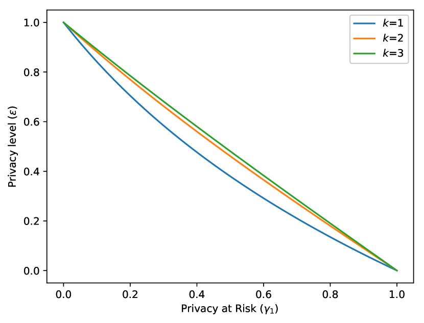
Figure 1:

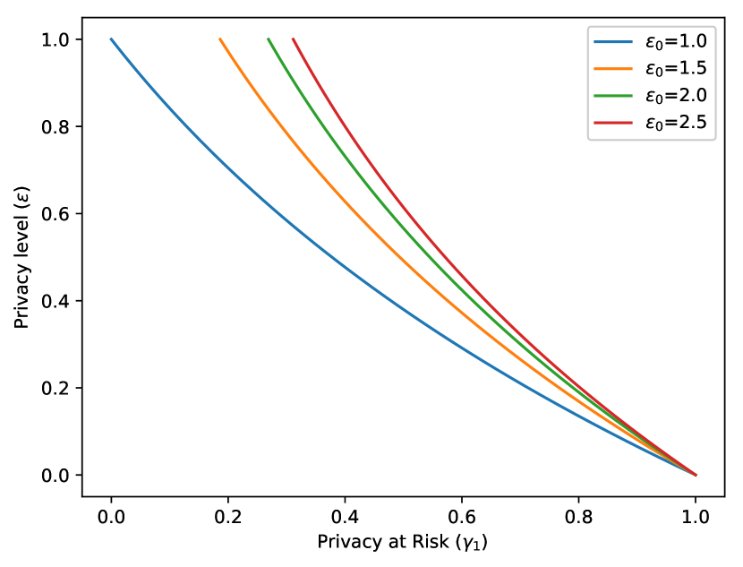
Figure 2:

Figure 3: Privacy level $\varepsilon$ for varying privacy at risk $\gamma_{1}$ for Laplace mechanism $\mathcal{L}_{\varepsilon_{0}}^{1.0}$. In Figure 1, we use $\varepsilon_{0}=1.0$ and different values of $k$. In Figure 2, for $k=1$ and different values of $\varepsilon_{0}$.

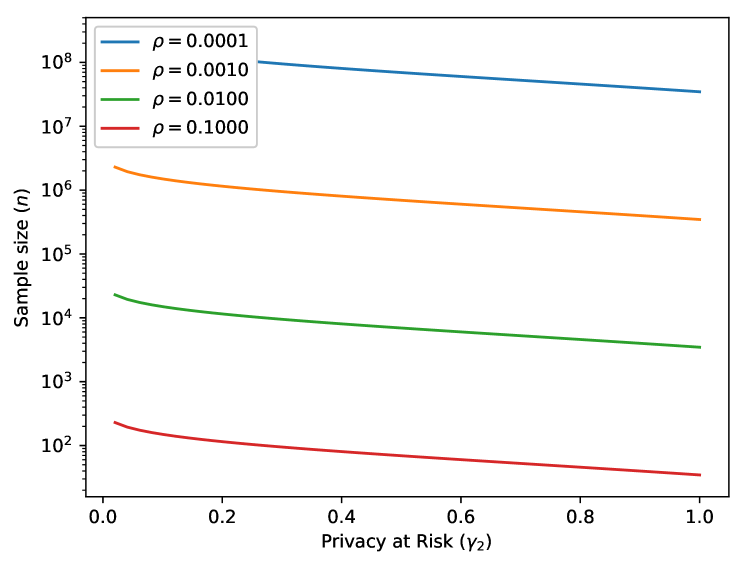
Figure 4: Number of samples $n$ for varying privacy at risk $\gamma_{2}$ for different error parameter $\rho$.

Result for a Real-valued Query. For the case $k=1$, the analytical derivation is fairly straightforward. In this case, we obtain an invertible closed-form of a privacy level for a specified risk. It is presented in Equation 4.

$$\varepsilon=\ln{\left(\frac{1}{1-\gamma_{1}(1-e^{-\varepsilon_{0}})}\right)}$$ (4)

Remarks on $\varepsilon_{0}$. For $k=1$, Figure 2 shows the plot of privacy at risk level $\varepsilon$ versus privacy at risk $\gamma_{1}$ for the Laplace mechanism $\mathcal{L}^{1.0}_{\varepsilon_{0}}$. As the value of $\varepsilon_{0}$ increases, the probability of Laplace mechanism generating higher value of noise reduces. Therefore, for a fixed privacy level, privacy at risk increases with the value of $\varepsilon_{0}$. The same observation is made for $k>1$.

4.2 The Case of Implicit Randomness

In this section, we study the effect of the implicit randomness induced by the data-generation distribution to provide a fine tuning for the Laplace mechanism. We fine-tune the risk for a specified privacy level without assuming that the sensitivity of the query.

If one takes into account randomness induced by the data-generation distribution, all pairs of neighbouring datasets are not equally probable. This leads to estimation of sensitivity of a query for a specified data-generation distribution. If we have access to an analytical form of the data-generation distribution and to the query, we could analytically derive the sensitivity distribution for the query. In general, we have access to the datasets, but not the data-generation distribution that generates them. We, therefore, statistically estimate sensitivity by constructing an empirical distribution. We call the sensitivity value obtained for a specified risk from the empirical cumulative distribution of sensitivity the sampled sensitivity (Definition 14). However, the value of sampled sensitivity is simply an estimate of the sensitivity for a specified risk. In order to capture this additional uncertainty introduced by the estimation from the empirical sensitivity distribution rather than the true unknown distribution, we compute a lower bound on the accuracy of this estimation. This lower bound yields a probabilistic lower bound on the specified risk. We refer to it as empirical risk. For a specified absolute risk $\gamma_{2}$, we denote by $\hat{\gamma_{2}}$ corresponding empirical risk.

For the Laplace mechanism $\mathcal{L}_{\varepsilon}^{\Delta_{S_{f}}}$ calibrated with sampled sensitivity $\Delta_{S_{f}}$ and privacy level $\varepsilon$, we evaluate the empirical risk $\hat{\gamma_{2}}$. We present the result in Theorem 13. The proof is available in Appendix B.

Theorem 13

Analytical bound on the empirical risk, $\hat{\gamma_{2}}$, for Laplace mechanism $\mathcal{L}_{\varepsilon}^{\Delta_{S_{f}}}$ with privacy level $\varepsilon$ and sampled sensitivity $\Delta_{S_{f}}$ for a query $f:\mathcal{D}\rightarrow\mathbb{R}^{k}$ is

$$\hat{\gamma_{2}}\geq\gamma_{2}(1-2e^{-2\rho^{2}n})$$ (5)

where $n$ is the number of samples used for estimation of the sampled sensitivity and $\rho$ is the accuracy parameter. $\gamma_{2}$ denotes the specified absolute risk.

The error parameter $\rho$ controls the closeness between the empirical cumulative distribution of the sensitivity to the true cumulative distribution of the sensitivity. Lower the value of the error, closer is the empirical cumulative distribution to the true cumulative distribution. Figure 4 shows the plot of number of samples as a function of the privacy at risk and the error parameter. Naturally, we require higher number of samples in order to have lower error rate. The number of samples reduces as the privacy at risk increases. The lower risk demands precision in the estimated sampled sensitivity, which in turn requires larger number of samples.

Let, $\mathcal{G}$ denotes the data-generation distribution, either known apriori or constructed by subsampling the available data. We adopt the procedure of (Rubinstein and Aldà, 2017) to sample two neighbouring datasets with $p$ data points each. We sample $p-1$ data points from $\mathcal{G}$ that are common to both of these datasets and later two more data points. From those two points, we allot one data point to each of the two datasets.

Let, $S_{f}=\lVert f(x)-f(y)\rVert_{1}$ denotes the sensitivity random variable for a given query $f$, where $x$ and $y$ are two neighbouring datasets sampled from $\mathcal{G}$. Using $n$ pairs of neighbouring datasets sampled from $\mathcal{G}$, we construct the empirical cumulative distribution, $F_{n}$, for the sensitivity random variable.

Definition 14

For a given query $f$ and for a specified risk $\gamma_{2}$, sampled sensitivity, $\Delta_{S_{f}}$, is defined as the value of sensitivity random variable that is estimated using its empirical cumulative distribution function, $F_{n}$, constructed using $n$ pairs of neighbouring datasets sampled from the data-generation distribution $\mathcal{G}$.

$$\Delta_{S_{f}}\triangleq F_{n}^{-1}(\gamma_{2})$$

If we knew analytical form of the data generation distribution, we could analytically derive the cumulative distribution function of the sensitivity, $F$, and find the sensitivity of the query as $\Delta_{f}=F^{-1}(1)$. Therefore, in order to have the sampled sensitivity close to the sensitivity of the query, we require the empirical cumulative distributions to be close to the cumulative distribution of the sensitivity. We use this insight to derive the analytical bound in the Theorem 13.

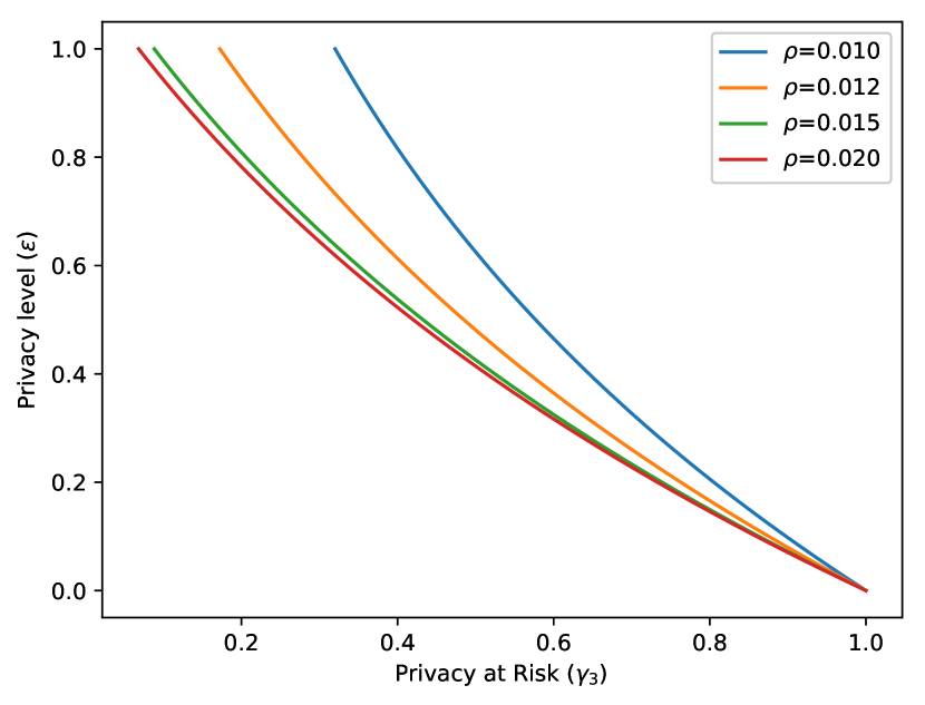
Figure 5:

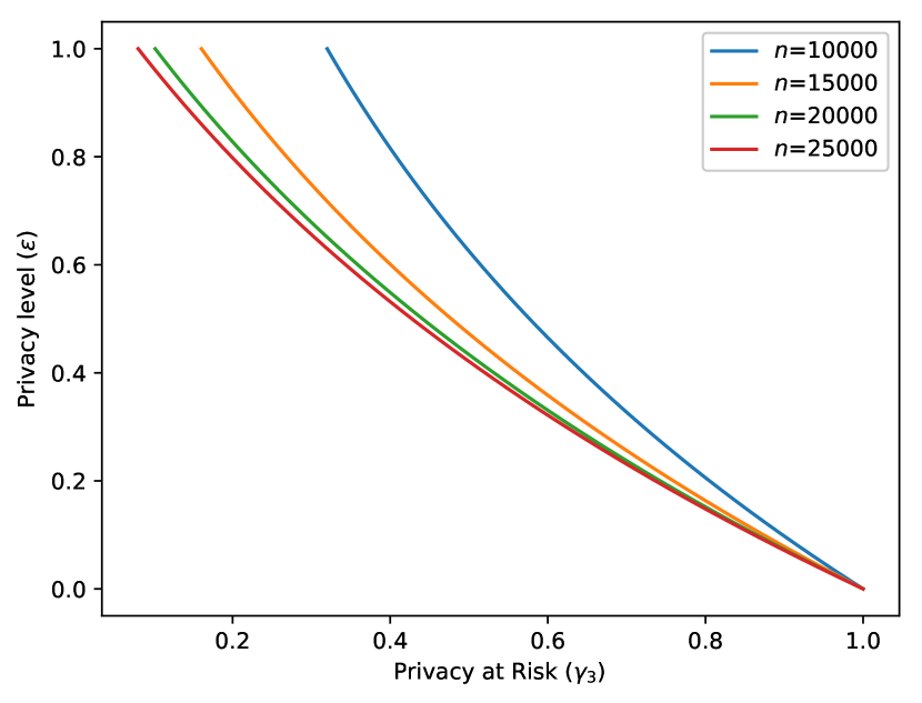
Figure 6:

Figure 7: Dependence of error and number of samples on the privacy at risk for Laplace mechanism $\mathcal{L}_{1.0}^{\Delta_{S_{f}}}$. For the figure on the left hand side, we fix the number of samples to $10000$. For the Figure 6 we fix the error parameter to $0.01$.

4.3 The Case of Explicit and Implicit Randomness

In this section, we study the combined effect of both explicit randomness induced by the noise distribution and implicit randomness in the data-generation distribution respectively. We do not assume the knowledge of the sensitivity of the query.

We estimate sensitivity using the empirical cumulative distribution of sensitivity. We construct the empirical distribution over the sensitivities using the sampling technique presented in the earlier case. Since we use the sampled sensitivity (Definition 14) to calibrate the Laplace mechanism, we estimate the empirical risk $\hat{\gamma_{3}}$.

For Laplace mechanism $\mathcal{L}_{\varepsilon_{0}}^{\Delta_{S_{f}}}$ calibrated with sampled sensitivity $\Delta_{S_{f}}$ and privacy level $\varepsilon_{0}$, we present the analytical bound on the empirical sensitivity $\hat{\gamma_{3}}$ in Theorem 15 with proof in the Appendix C.

Theorem 15

Analytical bound on the empirical risk $\hat{\gamma_{3}}\in[0,1]$ to achieve a privacy level $\varepsilon>0$ for Laplace mechanism $\mathcal{L}_{\varepsilon_{0}}^{\Delta_{S_{f}}}$ with sampled sensitivity $\Delta_{S_{f}}$ of a query $f:\mathcal{D}\rightarrow\mathbb{R}^{k}$ is

$$\hat{\gamma_{3}}\geq\gamma_{3}(1-2e^{-2\rho^{2}n})$$ (6)

where $n$ is the number of samples used for estimating the sensitivity, $\rho$ is the accuracy parameter. $\gamma_{3}$ denotes the specified absolute risk defined as:

$$\gamma_{3}=\frac{\mathbb{P}(T\leq\varepsilon)}{\mathbb{P}(T\leq\eta\varepsilon_{0})}\cdot\gamma_{2}$$

The error parameter $\rho$ controls the closeness between the empirical cumulative distribution of the sensitivity to the true cumulative distribution of the sensitivity. Figure 7 shows the dependence of the error parameter on the number of samples. In Figure 5, we observe that the for a fixed number of samples and a privacy level, the privacy at risk decreases with the value of error parameter. For a fixed number of samples, smaller values of the error parameter reduce the probability of similarity between the empirical cumulative distribution of sensitivity and the true cumulative distribution. Therefore, we observe the reduction in the risk for a fixed privacy level. In Figure 6, we observe that for a fixed value of error parameter and a fixed level of privacy level, the risk increases with the number of samples. For a fixed value of the error parameter, larger values of the sample size increase the probability of similarity between the empirical cumulative distribution of sensitivity and the true cumulative distribution. Therefore, we observe the increase in the risk for a fixed privacy level.

Effect of the consideration of implicit and explicit randomness is evident in the analytical expression for $\gamma_{3}$ in Equation 7. Proof is available in Appendix C. The privacy at risk is composed of two factors whereas the second term is a privacy at risk that accounts for inherent randomness. The first term takes into account the implicit randomness of the Laplace distribution along with a coupling coefficient $\eta$. We define $\eta$ as the ratio of the true sensitivity of the query to its sampled sensitivity.

$$\gamma_{3}\triangleq\frac{\mathbb{P}(T\leq\varepsilon)}{\mathbb{P}(T\leq\eta\varepsilon_{0})}\cdot\gamma_{2}$$ (7)

5 Minimising Compensation Budget for Privacy at Risk

Many service providers collect users’ data to enhance user experience. In order to avoid misuse of this data, we require a legal framework that not only limits the use of the collected data but also proposes reparative measures in case of a data leak. General Data Protection Regulation (GDPR) is such a legal framework.

Section 82 in GDPR states that any person who suffers from material or non-material damage as a result of a personal data breach has the right to demand compensation from the data processor. Therefore, every GDPR compliant business entity that either holds or processes personal data needs to secure a certain budget in the worst case scenario of the personal data breach. In order to reduce the risk of such an unfortunate event, the business entity may use privacy-preserving mechanisms that provide provable privacy guarantees while publishing their results. In order to calculate the compensation budget for a business entity, we devise a cost model that maps the privacy guarantees provided by differential privacy and privacy at risk to monetary costs. The discussions demonstrate the usefulness of probabilistic quantification of differential privacy in a business setting.

5.1 Cost Model for Differential Privacy

Let $E$ be the compensation budget that a business entity has to pay to every stakeholder in case of a personal data breach when the data is processed without any provable privacy guarantees. Let $E_{\varepsilon}^{dp}$ be the compensation budget that a business entity has to pay to every stakeholder in case of a personal data breach when the data is processed with privacy guarantees in terms of $\varepsilon$-differential privacy.

Privacy level, $\varepsilon$, in $\varepsilon$-differential privacy is the quantifier of indistinguishability of the outputs of a privacy-preserving mechanism when two neighbouring datasets are provided as inputs. When the privacy level is zero, the privacy-preserving mechanism outputs all results with equal probability. The indistinguishability reduces with increase in the privacy level. Thus, privacy level of zero bears the lowest risk of personal data breach and the risk increases with the privacy level. $E_{\varepsilon}^{dp}$ needs to be commensurate to such a risk and, therefore, it needs to satisfy the following constraints.

1. For all $\varepsilon\in\mathbb{R}^{\geq 0}$, $E_{\varepsilon}^{dp}\leq E$.

2. $E_{\varepsilon}^{dp}$ is a monotonically increasing function of $\varepsilon$.

3. As $\varepsilon\rightarrow 0$, $E_{\varepsilon}^{dp}\rightarrow E_{min}$ where $E_{min}$ is the unavoidable cost that business entity might need to pay in case of personal data breach even after the privacy measures are employed.

4. As $\varepsilon\rightarrow\infty$, $E_{\varepsilon}^{dp}\rightarrow E$.

There are various functions that satisfy these constraints. For instantiation, we choose to work with a cost model that is convex with respect to $\varepsilon$. The cost model $E_{\varepsilon}^{dp}$ as defined in Equation 8.

$$E_{\varepsilon}^{dp}\triangleq E_{min}+Ee^{-\frac{c}{\varepsilon}}$$ (8)

$E_{\varepsilon}^{dp}$ has two parameters, namely $c>0$ and $E_{min}\geq 0$. $c$ controls the rate of change in the cost as the privacy level changes and $E_{min}$ is a privacy level independent bias. For this study, we use a simplified model with $c=1$ and $E_{min}=0$.

5.2 Cost Model for Privacy at Risk

Let $E_{\varepsilon_{0}}^{par}(\varepsilon,\gamma)$ be the compensation that a business entity has to pay to every stakeholder in case of a personal data breach when the data is processed with an $\varepsilon_{0}$-differentially private privacy-preserving mechanism along with a probabilistic quantification of privacy level. Use of such a quantification allows use to provide a stronger a stronger privacy guarantee viz. $\varepsilon<\varepsilon_{0}$ for a specified privacy at risk at most $\gamma$ for Thus, we calculate $E_{\varepsilon_{0}}^{par}$ using Equation 9.

$$E_{\varepsilon_{0}}^{par}(\varepsilon,\gamma)\triangleq\gamma E_{\varepsilon}^{dp}+(1-\gamma)E_{\varepsilon_{0}}^{dp}$$ (9)

5.2.1 Existence of Minimum Compensation Budget

We want to find the privacy level, say $\varepsilon_{min}$, that yields the lowest compensation budget. We do that by minimising Equation 9 with respect to $\varepsilon$.

Lemma 16

$E_{\varepsilon_{0}}^{par}(\varepsilon,\gamma)$ is a convex function of $\varepsilon$ if $E_{\varepsilon}^{dp}$ is defined by Equation (9).

This result also generalises to any other convex cost model satisfying the four conditions. By Lemma 16, there exists a unique $\varepsilon_{min}$ that minimises the compensation budget for a specified parametrisation, say $\varepsilon_{0}$. Since the risk $\gamma$ in Equation 9 is itself a function of privacy level $\varepsilon$, analytical calculation of $\varepsilon_{min}$ is not possible in the most general case. When the output of the query is a real number, we derive the analytic form (Equation 4) to compute the risk under the consideration of explicit randomness. In such a case, $\varepsilon_{min}$ is calculated by differentiating Equation 9 with respect to $\varepsilon$ and equating it to zero. It gives us Equation 10 that we solve using any root finding technique such as Newton-Raphson method (Press, 2007) to compute $\varepsilon_{min}$.

$$\frac{1}{\varepsilon}-\ln{\left(1-\frac{1-e^{\varepsilon}}{\varepsilon^{2}}\right)}=\frac{1}{\varepsilon_{0}}$$ (10)

5.2.2 Fine-tuning Privacy at Risk

For a fixed budget, say $B$, re-arrangement of Equation 9 gives us an upper bound on the privacy level $\varepsilon$. We use the cost model with $c=1$ and $E_{min}=0$ to derive the upper bound. If we have a maximum permissible expected mean absolute error $T$, we use Equation 12 to obtain a lower bound on the privacy at risk level. Equation 11 illustrates the upper and lower bounds that dictate the permissible range of $\varepsilon$ that a data publisher can promise depending on the budget and the permissible error constraints.

$$\frac{1}{T}\leq\varepsilon\leq\left[\ln{\left(\frac{\gamma E}{B-(1-\gamma)E_{\varepsilon_{0}}^{dp}}\right)}\right]^{-1}$$ (11)

Thus, the privacy level is constrained by the effectiveness requirement from below and by the monetary budget from above. (Hsu et al., 2014) calculate upper and lower bound on the privacy level in the differential privacy. They use a different cost model owing to the scenario of research study that compensates its participants for their data and releases the results in a differentially private manner. Their cost model is different than our GDPR inspired modelling.

5.3 Illustration

Suppose that the health centre in a university that complies to GDPR publishes statistics of its staff health checkup, such as obesity statistics, twice in a year. In January 2018, the health centre publishes that 34 out of 99 faculty members suffer from obesity. In July 2018, the health centre publishes that 35 out of 100 faculty members suffer from obesity. An intruder, perhaps an analyst working for an insurance company, checks the staff listings in January 2018 and July 2018, which are publicly available on website of the university. The intruder does not find any change other than the recruitment of John Doe in April 2018. Thus, with high probability, the intruder deduces that John Doe suffers from obesity. In order to avoid such a privacy breach, the health centre decides to publish the results using the Laplace mechanism. In this case, the Laplace mechanism operates on the count query.

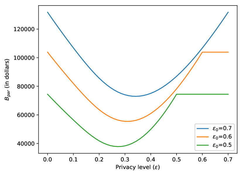
Figure 8: Variation in the budget for Laplace mechanism $\mathcal{L}_{\varepsilon_{0}}^{1}$ under privacy at risk considering explicit randomness in the Laplace mechanism for the illustration in Section 5.3.

In order to control the amount of noise, the health centre needs to appropriately set the privacy level. Suppose that the health centre decides to use the expected mean absolute error, defined in Equation 12, as the measure of effectiveness for the Laplace mechanism.

$$\mathbb{E}\left[\lvert\mathcal{L}^{1}_{\varepsilon}(x)-f(x)\rvert\right]=\frac{1}{\varepsilon}$$ (12)

Equation 12 makes use of the fact that the sensitivity of the count query is one. Suppose that the health centre requires the expected mean absolute error of at most two in order to maintain the quality of the published statistics. In this case, the privacy level has to be at least $0.5$.

In order to compute the budget, the health centre requires an estimate of $E$. Moriarty et al. (2012) shows that the incremental cost of premiums for the health insurance with morbid obesity ranges between $\$5467$ to $\$5530$. With reference to this research, the health centre takes $\$5500$ as an estimate of $E$. For the staff size of $100$ and the privacy level $0.5$, the health centre uses Equation 8 in its simplified setting to compute the total budget of $\$74434.40$.

Is it possible to reduce this budget without degrading the effectiveness of the Laplace mechanism? We show that it is possible by fine-tuning the Laplace mechanism. Under the consideration of the explicit randomness introduced by the Laplace noise distribution, we show that $\varepsilon_{0}$-differentially private Laplace mechanism also satisfies $\varepsilon$-differential privacy with risk $\gamma$, which is computed using the formula in Theorem 12. Fine-tuning allows us to get a stronger privacy guarantee, $\varepsilon<\varepsilon_{0}$ that requires a smaller budget. In Figure 8, we plot the budget for various privacy levels. We observe that the privacy level $0.274$, which is same as $\varepsilon_{min}$ computed by solving Equation 10, yields the lowest compensation budget of $\$37805.86$. Thus, by using privacy at risk, the health centre is able to save $\$36628.532$ without sacrificing the quality of the published results.

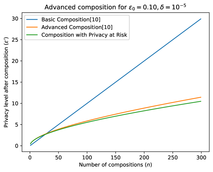
Figure 9: $\mathcal{L}_{0.1}^{1}$ satisfies $(0.08,0.80)$-privacy at risk.

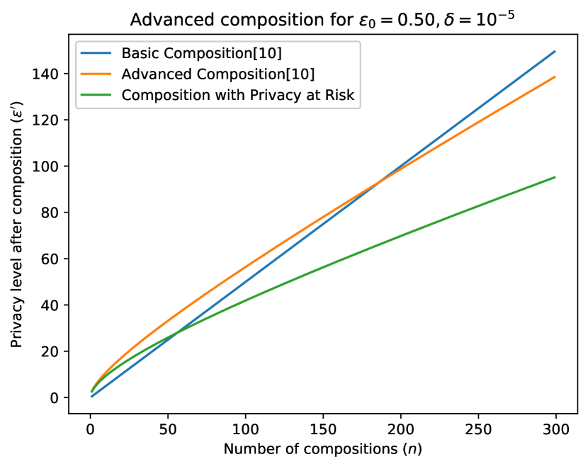
Figure 10: $\mathcal{L}_{0.5}^{1}$ satisfies $(0.27,0.61)$-privacy at risk.

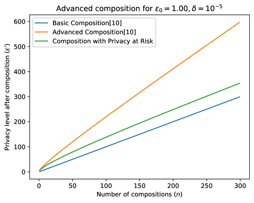
Figure 11: $\mathcal{L}_{1.0}^{1}$ satisfies $(0.42,0.54)$-privacy at risk.

Figure 12: Comparing the privacy guarantee obtained by basic composition and advanced composition (Dwork et al., 2014) with the composition obtained using optimal privacy at risk that minimises the cost of Laplace mechanism $\mathcal{L}_{\varepsilon_{0}}^{1}$. For the evaluation, we set $\delta=10^{-5}$.

5.4 Cost Model and the Composition of Laplace Mechanisms

Convexity of the proposed cost function enables us to estimate the optimal value of the privacy at risk level. We use the optimal privacy value to provide tighter bounds on the composition of Laplace mechanism. In Figure 12, we compare the privacy guarantees obtained by using basic composition theorem (Dwork et al., 2014), advanced composition theorem (Dwork et al., 2014) and the composition theorem for privacy at risk. We comparatively evaluate them for composition of Laplace mechanisms with privacy levels $0.1,0.5$ and $1.0$. We compute the privacy level after composition by setting $\delta$ to $10^{-5}$.

We observe that the use of optimal privacy at risk provided significantly stronger privacy guarantees as compared to the conventional composition theorems. Advanced composition theorem is known to provide stronger privacy guarantees for mechanism with smaller $\varepsilon$s. As we observe in Figure 11 and Figure 10, the composition provides strictly stronger privacy guarantees than basic composition, in the cases where the advanced composition fails.

6 Balancing Utility and Privacy

In this section, we empirically illustrate and discuss the steps that a data steward needs to take and the issues that she needs to consider in order to realise a required privacy at risk level $\varepsilon$ for a confidence level $\gamma$ when seeking to disclose the result of a query.

We consider a query that returns the parameter of a ridge regression (Murphy, 2012) for an input dataset. It is a basic and widely used statistical analysis tool. We use the privacy-preserving mechanism presented by Ligett et al. for ridge regression. It is a Laplace mechanism that induces noise in the output parameters of the ridge regression. The authors provide a theoretical upper bound on the sensitivity of the ridge regression, which we refer as sensitivity, in the experiments.

6.1 Dataset and Experimental Setup

We conduct experiments on a subset of the 2000 US census dataset provided by Minnesota Population Center in its Integrated Public Use Microdata Series (Ruggles et al., 2015). The census dataset consists of 1% sample of the original census data. It spans over 1.23 million households with records of 2.8 million people. The value of several attributes is not necessarily available for every household. We have therefore selected $212,605$ records, corresponding to the household heads, and $6$ attributes, namely, Age, Gender, Race, Marital Status, Education, Income, whose values are available for the $212,605$ records.

In order to satisfy the constraint in the derivation of the sensitivity of ridge regression (Ligett et al., 2017), we, without loss of generality, normalise the dataset in the following way. We normalise Income attribute such that the values lie in $[0,1]$. We normalise other attributes such that $l_{2}$ norm of each data point is unity.

All experiments are run on Linux machine with 12-core 3.60GHz Intel^® Core i7™processor with 64GB memory. Python^® 2.7.6 is used as the scripting language.

6.2 Result Analysis

We train ridge regression model to predict Income using other attributes as predictors. We split the dataset into the training dataset ($80\%$) and testing dataset ($20\%$). We compute the root mean squared error (RMSE) of ridge regression, trained on the training data with regularisation parameter set to $0.01$, on the testing dataset. We use it as the metric of utility loss. Smaller the value of RMSE, smaller the loss in utility. For a given value of privacy at risk level, we compute $50$ runs of an experiment of a differentially private ridge regression and report the means over the $50$ runs of the experiment.

Let us now provide illustrative experiments under the three different cases. In every scenario, the data steward is given a privacy at risk level $\varepsilon$ and the confidence level $\gamma$ and wants to disclose the parameters of a ridge regression model that she trains on the census dataset. She needs to calibrate the Laplace mechanism to achieve the privacy at risk required the ridge regression query.

The Case of Explicit Randomness (cf. Section 4.1). In this scenario, the data steward knows the sensitivity for the ridge regression. She needs to compute the privacy level, $\varepsilon_{0}$, to calibrate the Laplace mechanism. She uses Equation 3 that links the desired privacy at risk level $\varepsilon$, the confidence level $\gamma_{1}$ and the privacy level of noise $\varepsilon_{0}$. Specifically, for given $\varepsilon$ and $\gamma_{1}$, she computes $\varepsilon_{0}$ by solving the equation:

$$\gamma_{1}\mathbb{P}(T\leq\varepsilon_{0})-\mathbb{P}(T\leq\varepsilon)=0.$$

Since the equation does not give an analytical formula for $\varepsilon_{0}$, the data steward uses a root finding algorithm such as Newton-Raphson method (Press, 2007) to solve the above equation. For instance, if she needs to achieve a privacy at risk level $\varepsilon=0.4$ with confidence level $\gamma_{1}=0.6$, she can substitute these values in the above equation and solve the equation to get the privacy level of noise $\varepsilon_{0}=0.8$.

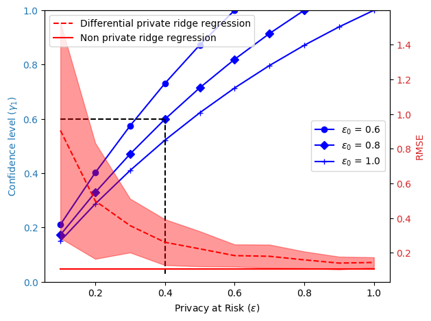
Figure 13: Utility, measured by RMSE (right y-axis), and privacy at risk level $\varepsilon$ for Laplace mechanism (left y-axis) for varying confidence levels $\gamma_{1}$.

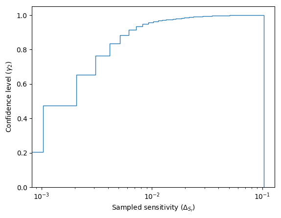
Figure 14: Empirical cumulative distribution of the sensitivities of ridge regression queries constructed using $15000$ samples of neighboring datasets.

Figure 13 shows the variation of privacy at risk level $\varepsilon$ and confidence level $\gamma_{1}$. It also depicts the variation of utility loss for different privacy at risk levels in Figure 13.

In accordance to the data steward’s problem, if she needs to achieve a privacy at risk level $\varepsilon=0.4$ with confidence level $\gamma_{1}=0.6$, she obtains the privacy level of noise to be $\varepsilon_{0}=0.8$. Additionally, we observe that the choice of privacy level $0.8$ instead of $0.4$ to calibrate the Laplace mechanism gives lower utility loss for the data steward. This is the benefit drawn from the risk taken under the control of privacy at risk.

Thus, she uses privacy level $\varepsilon_{0}$ and the sensitivity of the function to calibrate Laplace mechanism.

The Case of Implicit Randomness (cf. Section 4.2). In this scenario, the data steward does not know the sensitivity of ridge regression. She assesses that she can afford to sample at most $n$ times from the population dataset. She understands the effect of the uncertainty introduced by the statistical estimation of the sensitivity. Therefore, she uses the confidence level for empirical privacy at risk $\hat{\gamma_{2}}$.

Given the value of $n$, she chooses the value of the accuracy parameter using Figure 4. For instance, if the number of samples that she can draw is $10^{4}$, she chooses the value of the accuracy parameter $\rho=0.01$. Next, she uses Equation 13 to determine the value of probabilistic tolerance, $\alpha$, for the sample size $n$. For instance, if the data steward is not allowed to access more than $15,000$ samples, for the accuracy of $0.01$ the probabilistic tolerance is $0.9$.

$$\alpha=1-2e^{(-2\rho^{2}n)}$$ (13)

She constructs an empirical cumulative distribution over the sensitivities as described in Section 4.2. Such an empirical cumulative distribution is shown in Figure 14. Using the computed probabilistic tolerance and desired confidence level $\hat{\gamma_{2}}$, she uses equation in Theorem 13 to determine $\gamma_{2}$. She computes the sampled sensitivity using the empirical distribution function and the confidence level for privacy $\Delta_{S_{f}}$ at risk $\gamma_{2}$. For instance, using the empirical cumulative distribution in Figure 14 she calculates the value of the sampled sensitivity to be approximately $0.001$ for $\gamma_{2}=0.4$ and approximately $0.01$ for $\gamma_{2}=0.85$

Thus, she uses privacy level $\varepsilon$, sets the number of samples to be $n$ and computes the sampled sensitivity $\Delta_{S_{f}}$ to calibrate the Laplace mechanism.

The Case of Explicit and Implicit Randomness (cf. Section 4.3). In this scenario, the data steward does not know the sensitivity of ridge regression. She is not allowed to sample more than $n$ times from a population dataset. For a given confidence level $\gamma_{2}$ and the privacy at risk $\varepsilon$, she calibrates the Laplace mechanism using illustration for Section 4.3. The privacy level in this calibration yields utility loss that is more than her requirement. Therefore, she wants to re-calibrate the Laplace mechanism in order to reduce utility loss.

For the re-calibration, the data steward uses privacy level of the pre-calibrated Laplace mechanism, i.e. $\varepsilon$, as the privacy at risk level and she provides a new confidence level for empirical privacy at risk $\hat{\gamma_{3}}$. Using Equation 26 and Equation 24, she calculates:

$$\hat{\gamma_{3}}\mathbb{P}(T\leq\eta\varepsilon_{0})-\alpha\gamma_{2}~{}\mathbb{P}(T\leq\varepsilon)=0$$

She solves such an equation for $\varepsilon_{0}$ using the root finding technique such as Newton-Raphson method (Press, 2007). For instance, if she needs to achieve a privacy at risk level $\varepsilon=0.4$ with confidence levels $\hat{\gamma_{3}}=0.9$ and $\gamma_{2}=0.9$, she can substitute these values and the values of tolerance parameter and sampled sensitivity, as used in the previous experiments, in the above equation. Then, solving the equation leads to the privacy level of noise $\varepsilon_{0}=0.8$.

Thus, she re-calibrates the Laplace mechanism with privacy level $\varepsilon_{0}$, sets the number of samples to be $n$ and sampled sensitivity $\Delta_{S_{f}}$.

7 Related Work

Calibration of mechanisms. Researchers have proposed different privacy-preserving mechanisms to make different queries differentially private. These mechanisms can be broadly classified into two categories. In one category, the mechanisms explicitly add calibrated noise, such as Laplace noise in the work of (Dwork et al., 2006c) or Gaussian noise in the work of (Dwork et al., 2014), to the outputs of the query. In the other category, (Chaudhuri et al., 2011; Zhang et al., 2012; Acs et al., 2012; Hall et al., 2013) propose mechanisms that alter the query function so that the modified function satisfies differentially privacy. Privacy-preserving mechanisms in both of these categories perturb the original output of the query and make it difficult for a malicious data analyst to recover the original output of the query. These mechanisms induce randomness using the explicit noise distribution. Calibration of these mechanisms require the knowledge of the sensitivity of the query. Nissim et al. consider the implicit randomness in the data-generation distribution to compute an estimate of the sensitivity. The authors propose the smooth sensitivity function that is an envelope over the local sensitivities for all individual datasets. Local sensitivity of a dataset is the maximum change in the value of the query over all of its neighboring datasets. In general, it is not easy to analytically estimate the smooth sensitivity function for a general query. Rubinstein and Aldà also study the inherent randomness in the data-generation algorithm. They do not use the local sensitivity. We adopt their approach of sampling the sensitivity from the empirical distribution of the sensitivity. They use order statistics to choose a particular value of the sensitivity. We use the risk, which provides a mediation tool for business entities to assess the actual business risks, on the sensitivity distribution to estimate the sensitivity.

Refinements of differential privacy. In order to account for both sources of randomness, refinements of $\varepsilon$-differential privacy are proposed in order to bound the probability of occurrence of worst case scenarios. Machanavajjhala et al. propose probabilistic differential privacy that considers upper bounds of the worst case privacy loss for corresponding confidence levels on the noise distribution. Definition of probabilistic differential privacy incorporates the explicit randomness induced by the noise distribution and bounds the probability over the space of noisy outputs to satisfy the $\varepsilon$-differential privacy definition. Dwork and Rothblum propose Concentrated differential privacy that considers the expected values of the privacy loss random variables for the corresponding. Definition of concentrated differential privacy incorporates the explicit randomness induced by the noise distribution but considering only the expected value of privacy loss satisfying $\varepsilon$-differential privacy definition instead of using the confidence levels limits its scope.

Hall et al. propose random differential privacy that considers the privacy loss for corresponding confidence levels on the implicit randomness in the data-generation distribution. Definition of random differential privacy incorporates the implicit randomness induced by the data-generation distribution and bounds the probability over the space of datasets generated from the given distribution to satisfy the $\varepsilon$-differential privacy definition. Dwork et al. define approximate differential privacy by adding a constant bias to the privacy guarantee provided by the differential privacy. It is not a probabilistic refinement of the differential privacy.

Around the same time of our work, Triastcyn and Faltings independently propose Bayesian differential privacy that takes into account both of the sources of randomness. Despite this similarity, our works differ in multiple dimensions. Firstly, they have shown the reduction of their definition to a variant of Renyi differential privacy that depends on the data-generation distribution. Secondly, they rely on the moment accountant for the composition of the mechanisms. Lastly, they do not provide a finer case-by-case analysis of the source of randomness, which leads to analytical solutions for the privacy guarantee.

Kifer and Machanavajjhala define Pufferfish privacy framework, and its variant by Bassily et al., that considers randomness due to data-generation distribution as well as noise distribution. Despite the generality of their approach, the framework relies on the domain expert to define a set of secrets that they want to protect.

Composition theorem. Recently proposed technique of the moment accountant (Abadi et al., 2016) has become the state-of-the-art of composing mechanisms in the area of privacy-preserving machine learning. Abadi et al. show that the moment accountant provides much strong privacy guarantees than the conventional composition mechanisms. It works by keeping track of various moments of privacy loss random variable and use the bounds on them to provide privacy guarantees. The moment accountant requires access to data-generation distribution to compute the bounds on the moment. Hence, the privacy guarantees are specific to the dataset.

Cost models. (Ghosh and Roth, 2015; Chen et al., 2016) propose game theoretic methods that provide the means to evaluate the monetary cost of differential privacy. Our approach is inspired by the approach in the work of Hsu et al.. They model the cost under a scenario of a research study wherein the participants are reimbursed for their participation. Our cost modelling is driven by the scenario of securing a compensation budget in compliance with GDPR. Our requirement differs from the requirements for the scenario in their work. In our case, there is no monetary incentive for participants to share their data.

8 Conclusion and Future Works

In this paper, we provide a means to fine-tune the privacy level of a privacy-preserving mechanism by analysing various sources of randomness. Such a fine-tuning leads to probabilistic quantification on privacy levels with quantified risks, which we call as privacy at risk. We also provide composition theorem that leverages privacy at risk. We analytical calculate privacy at risk for Laplace mechanism. We propose a cost model that bridges the gap between the privacy level and the compensation budget estimated by a GDPR compliant business entity. Convexity of the cost function ensures existence of unique privacy at risk that minimises compensation budget. The cost model helps in not only reinforcing the ease of application in a business setting but also providing stronger privacy guarantees on the composition of mechanism.

Privacy at risk may be fully analytically computed in cases where the data-generation, or the sensitivity distribution, the noise distribution and the query are analytically known and take convenient forms. We are now looking at such convenient but realistic cases.

A Proof of Theorem 12 (Section 4.1)

Although a Laplace mechanism $\mathcal{L}^{\Delta_{f}}_{\varepsilon}$ induces higher amount of noise on average than a Laplace mechanism $\mathcal{L}^{\Delta_{f}}_{\varepsilon_{0}}$ for $\varepsilon<\varepsilon_{0}$, there is a non-zero probability that $\mathcal{L}^{\Delta_{f}}_{\varepsilon}$ induces noise commensurate to $\mathcal{L}^{\Delta_{f}}_{\varepsilon_{0}}$. This non-zero probability guides us to calculate the privacy at risk $\gamma_{1}$ for the privacy at risk level $\varepsilon$. In order to get an intuition, we illustrate the calculation of the overlap between two Laplace distributions as an estimator of similarity between the two distributions.

Definition 17

[Overlap of Distributions, (Papoulis and Pillai, 2002)] The overlap, $O$, between two probability distributions $P_{1},P_{2}$ with support $\mathcal{X}$ is defined as

$$O=\int_{\mathcal{X}}\min[P_{1}(x),P_{2}(x)]~{}{dx}.$$

Lemma 18

The overlap $O$ between two probability distributions, $\mathrm{Lap}(\frac{\Delta_{f}}{\varepsilon_{1}})$ and $\mathrm{Lap}(\frac{\Delta_{f}}{\varepsilon_{2}})$, such that $\varepsilon_{2}\leq\varepsilon_{1}$, is given by

$$O=1-(\exp{(-\mu\varepsilon_{2}/\Delta_{f})}-\exp{(-\mu\varepsilon_{1}/\Delta_{f})}),$$

where $\mu=\frac{\Delta_{f}\ln{(\varepsilon_{1}/\varepsilon_{2})}}{\varepsilon_{1}-\varepsilon_{2}}$.

Using the result in Lemma 18, we note that the overlap between two distributions with $\varepsilon_{0}=1$ and $\varepsilon=0.6$ is $0.81$. Thus, $\mathcal{L}^{\Delta_{f}}_{0.6}$ induces noise that is more than $80\%$ times similar to the noise induced by $\mathcal{L}^{\Delta_{f}}_{1.0}$. Therefore, we can loosely say that at least $80\%$ of the times a Laplace Mechanism $\mathcal{L}^{\Delta_{f}}_{1.0}$ will provide the same privacy as a Laplace Mechanism $\mathcal{L}^{\Delta_{f}}_{0.8}$.

Although the overlap between Laplace distributions with different scales offers an insight into the relationship between different privacy levels, it does not capture the constraint induced by the sensitivity. For a given query $f$, the amount of noise required to satisfy differential privacy is commensurate to the sensitivity of the query. This calibration puts a constraint on the noise that is required to be induced on a pair of neighbouring datasets. We state this constraint in Lemma 19, which we further use to prove that the Laplace Mechanism $\mathcal{L}^{\Delta_{f}}_{\varepsilon_{0}}$ satisfies $(\varepsilon,\gamma_{1})$-privacy at risk.

Lemma 19

For a Laplace Mechanism $\mathcal{L}^{\Delta_{f}}_{\varepsilon_{0}}$, the difference in the absolute values of noise induced on a pair of neighbouring datasets is upper bounded by the sensitivity of the query.

Proof  Suppose that two neighbouring datasets $x$ and $y$ are given input to a numeric query $f:\mathcal{D}\rightarrow\mathbb{R}^{k}$. For any output $z\in\mathbb{R}^{k}$ of the Laplace Mechanism $\mathcal{L}^{\Delta_{f}}_{\varepsilon_{0}}$,

$$\sum_{i=1}^{k}\left(|f(y_{i})-z_{i}|-|f(x_{i})-z_{i}|\right) \leq\sum_{i=1}^{k}\left(|f(x_{i})-f(y_{i})|\right)$$

$$\leq\Delta_{f}.$$

We use triangular inequality in the first step and Definition 2 of sensitivity in the second step.  

We write $\mathrm{Exp}(b)$ to denote a random variable sampled from an exponential distribution with scale $b>0$. We write $\mathrm{Gamma}(k,\theta)$ to denote a random variable sampled from a gamma distribution with shape $k>0$ and scale $\theta>0$.

Lemma 20

[(Papoulis and Pillai, 2002)] If a random variable $X$ follows Laplace Distribution with mean zero and scale $b$, $|X|\sim\mathrm{Exp}(b)$.

Lemma 21

[(Papoulis and Pillai, 2002)] If $X_{1},...,X_{n}$ are $n$ i.i.d. random variables each following the Exponential Distribution with scale $b$, $\sum_{i=1}^{n}X_{i}\sim\textrm{Gamma}(n,b)$.

Lemma 22

If $X_{1}$ and $X_{2}$ are two i.i.d. Gamma$(n,\theta)$ random variables, the probability density function for the random variable $T=|X_{1}-X_{2}|/\theta$ is given by

$$P_{T}(t;n,\theta)=\frac{2^{2-n}t^{n-\frac{1}{2}}K_{n-\frac{1}{2}}(t)}{\sqrt{2\pi}\Gamma(n)\theta}$$

where $K_{n-\frac{1}{2}}$ is the modified Bessel function of second kind.

Proof  Let $X_{1}$ and $X_{2}$ be two i.i.d. $\mathrm{Gamma}(n,\theta)$ random variables. Characteristic function of a Gamma random variable is given as

$$\phi_{X_{1}}(z)=\phi_{X_{2}}(z)=(1-\iota z\theta)^{-n}.$$

Therefore,

$$\phi_{X_{1}-X_{2}}(z)=\phi_{X_{1}}(z)\phi_{X_{2}}^{*}(z)=\frac{1}{(1+(z\theta)^{2})^{n}}$$

Probability density function for the random variable $X_{1}-X_{2}$ is given by,

$$P_{X_{1}-X_{2}}(x) =\frac{1}{2\pi}\int_{-\infty}^{\infty}e^{-\mathrm{i}zx}\phi_{X_{1}-X_{2}}(z)dz$$

$$=\frac{2^{1-n}{|\frac{x}{\theta}|}^{n-\frac{1}{2}}K_{n-\frac{1}{2}}(|\frac{x}{\theta}|)}{\sqrt{2\pi}\Gamma(n)\theta}$$

where $K_{n-\frac{1}{2}}$ is the Bessel function of second kind. Let $T=|\frac{X_{1}-X_{2}}{\theta}|$. Therefore,

$$P_{T}(t;n,\theta)=\frac{2^{1-n}t^{n-\frac{1}{2}}K_{n-\frac{1}{2}}(t)}{\sqrt{2\pi}\Gamma(n)\theta}$$

We use Mathematica (Inc., 2014) to solve the above integral.  

Lemma 23

If $X_{1}$ and $X_{2}$ are two i.i.d. Gamma$(n,\theta)$ random variables and $|X_{1}-X_{2}|\leq M$, then $T^{\prime}=|X_{1}-X_{2}|/\theta$ follows the distribution with probability density function:

$$P_{T^{\prime}}(t;n,\theta,M)=\frac{P_{T}(t^{\prime};n,\theta)}{P_{T}(T\leq M)},$$

where $P_{T}$ is the probability density function of defined in Lemma 22.

Lemma 24

For Laplace Mechanism $\mathcal{L}^{\Delta_{f}}_{\varepsilon_{0}}$ with query $f:\mathcal{D}\rightarrow\mathbb{R}^{k}$ and for any output $Z\subseteq Range(\mathcal{L}^{\Delta_{f}}_{\varepsilon_{0}})$, $\varepsilon\leq\varepsilon_{0}$,

$$\gamma_{1}\triangleq\mathbb{P}\left[\ln{\left|\frac{\mathbb{P}(\mathcal{L}^{\Delta_{f}}_{\varepsilon_{0}}(x)\in Z)}{\mathbb{P}(\mathcal{L}^{\Delta_{f}}_{\varepsilon_{0}}(y)\in Z)}\right|}\leq\varepsilon\right]=\frac{\mathbb{P}(T\leq\varepsilon)}{\mathbb{P}(T\leq\varepsilon_{0})},$$

where $T$ follows the distribution in Lemma 22, $P_{T}(t;k,\frac{\Delta_{f}}{\varepsilon_{0}})$.

Proof  Let, $x\in\mathcal{D}$ and $y\in\mathcal{D}$ be two datasets such that $x\sim y$. Let $f:\mathcal{D}\rightarrow\mathbb{R}^{k}$ be some numeric query. Let $\mathbb{P}_{x}(z)$ and $\mathbb{P}_{y}(z)$ denote the probabilities of getting the output $z$ for Laplace mechanisms $\mathcal{L}^{\Delta_{f}}_{\varepsilon_{0}}(x)$ and $\mathcal{L}^{\Delta_{f}}_{\varepsilon_{0}}(y)$ respectively. For any point $z\in\mathbb{R}^{k}$ and $\varepsilon\neq 0$,

$$~{}\frac{\mathbb{P}_{x}(z)}{\mathbb{P}_{y}(z)} =\prod_{i=1}^{k}\frac{\exp{\left(\frac{-\varepsilon_{0}|f(x_{i})-z_{i}|}{\Delta_{f}}\right)}}{\exp{\left(\frac{-\varepsilon_{0}|f(y_{i})-z_{i}|}{\Delta_{f}}\right)}}$$

$$=\prod_{i=1}^{k}\exp{\left(\frac{\varepsilon_{0}(|f(y_{i})-z_{i}|-|f(x_{i})-z_{i}|)}{\Delta_{f}}\right)}$$

$$=\exp{\left(\varepsilon\left[\frac{\varepsilon_{0}\sum_{i=1}^{k}(|f(y_{i})-z_{i}|-|f(x_{i})-z_{i}|)}{\varepsilon\Delta_{f}}\right]\right)}.$$ (14)

By Definition 4,

$$(f(x)-z),(f(y)-z)\sim\textrm{Lap}(\Delta_{f}/\varepsilon_{0}).$$ (15)

Application of Lemma 20 and Lemma 21 yields,

$$\sum_{i=1}^{k}\left(|f(x_{i})-z_{i}|\right)\sim\textrm{Gamma}(k,\Delta_{f}/\varepsilon_{0}).$$ (16)

Using Equations 15, 16, and Lemma 19,  23, we get

$$\left(\frac{\varepsilon_{0}}{\Delta_{f}}\sum_{i=1}^{k}\left|\left(|f(y_{i})-z|-|f(x_{i})-z|\right)\right|\right)\\ \sim P_{T^{\prime}}(t;k,\Delta_{f}/\varepsilon_{0},\Delta_{f}).$$ (17)

since, $\sum_{i=1}^{k}\left|\left(|f(y_{i})-z|-|f(x_{i})-z|\right)\right|\leq\Delta_{f}$. Therefore,

$$\mathbb{P}\left(\left[\frac{\varepsilon_{0}}{\Delta_{f}}\sum_{i=1}^{k}\ \left|\left(|f(y_{i})-z|-|f(x_{i})-z|\right)\right|\right]\leq\varepsilon\right)=\frac{\mathbb{P}(T\leq\varepsilon)}{\mathbb{P}(T\leq\varepsilon_{0})},$$ (18)

where $T$ follows the distribution in Lemma 22. We use Mathematica (Inc., 2014) to analytically compute,

$$\mathbb{P}(T\leq x)\propto\left({}_{1}F_{2}(\frac{1}{2};\frac{3}{2}-k,\frac{3}{2};\frac{x^{2}}{4})\sqrt{\pi}4^{k}x]\right)-\\ \left(2_{1}F_{2}(k;\frac{1}{2}+k,k+1;\frac{x^{2}}{4})x^{2k}\Gamma(k)\right)$$

where ${}_{1}F_{2}$ is the regularised generalised hypergeometric function as defined in (Askey and Daalhuis, 2010). From Equation A and 18,

$$\mathbb{P}\left[\ln{\left|\frac{\mathbb{P}(\mathcal{L}_{\varepsilon_{0}}^{\Delta_{f}}(x)\in S)}{\mathbb{P}(\mathcal{L}_{\varepsilon_{0}}^{\Delta_{f}}(y)\in S)}\right|}\leq\varepsilon\right]=\frac{\mathbb{P}(T\leq\varepsilon)}{\mathbb{P}(T\leq\varepsilon_{0})}.$$

 

This completes the proof of Theorem 12.

Corollary 25

Laplace Mechanism $\mathcal{L}^{\Delta_{f}}_{\varepsilon_{0}}$ with $f:\mathcal{D}\rightarrow\mathbb{R}^{k}$ is $(\varepsilon,\delta)$-probabilistically differentially private where

$$\delta=\begin{cases}1-\frac{\mathbb{P}(T\leq\varepsilon)}{\mathbb{P}(T\leq\varepsilon_{0})}&\quad\varepsilon\leq\varepsilon_{0}\\ 0&\quad\varepsilon>\varepsilon_{0}\end{cases}$$

and $T$ follows $\mathrm{BesselK}(k,\Delta_{f}/\varepsilon_{0})$.

B Proof of Theorem 13 (Section 4.2)

Proof  Let, $x$ and $y$ be any two neighbouring datasets sampled from the data generating distribution $\mathcal{G}$. Let, $\Delta_{S_{f}}$ be the sampled sensitivity for query $f:\mathcal{D}\rightarrow\mathbb{R}^{k}$. Let, $\mathbb{P}_{x}(z)$ and $\mathbb{P}_{y}(z)$ denote the probabilities of getting the output $z$ for Laplace mechanisms $\mathcal{L}_{\varepsilon}^{\Delta_{S_{f}}}(x)$ and $\mathcal{L}_{\varepsilon}^{\Delta_{S_{f}}}(y)$ respectively. For any point $z\in\mathbb{R}^{k}$ and $\varepsilon\neq 0$,

$$\frac{\mathbb{P}_{x}(z)}{\mathbb{P}_{y}(z)} =\prod_{i=1}^{k}\frac{\exp{\left(\frac{-\varepsilon|f(x_{i})-z_{i}|}{\Delta_{S_{f}}}\right)}}{\exp{\left(\frac{-\varepsilon|f(y_{i})-z_{i}|}{\Delta_{S_{f}}}\right)}}$$

$$=\exp{\left(\frac{\varepsilon\sum_{i=1}^{k}(|f(y_{i})-z_{i}|-|f(x_{i})-z_{i}|)}{\Delta_{S_{f}}}\right)}$$

$$\leq\exp{\left(\frac{\varepsilon\sum_{i=1}^{k}|f(y_{i})-f(x_{i})|}{\Delta_{S_{f}}}\right)}$$

$$=\exp{\left(\frac{\varepsilon\lVert f(y)-f(x)\rVert_{1}}{\Delta_{S_{f}}}\right)}$$ (19)

We used triangle inequality in the penultimate step.

Using the trick in the work of (Rubinstein and Aldà, 2017), we define following events. Let, $B^{\Delta_{S_{f}}}$ denotes the set of pairs neighbouring dataset sampled from $\mathcal{G}$ for which the sensitivity random variable is upper bounded by $\Delta_{S_{f}}$. Let, $C_{\rho}^{\Delta_{S_{f}}}$ denotes the set of sensitivity random variable values for which $F_{n}$ deviates from the unknown cumulative distribution of $S$, $F$, at most by the accuracy value $\rho$. These events are defined in Equation 20.

$$B^{\Delta_{S_{f}}} \triangleq\{x,y\sim\mathcal{G}~{}\textrm{such that}~{}\lVert f(y)-f(x)\rVert_{1}\leq\Delta_{S_{f}}\}$$

$$C_{\rho}^{\Delta_{S_{f}}} \triangleq\left\{\sup_{\Delta}|F_{S}^{n}(\Delta)-F_{S}(\Delta)|\leq\rho\right\}$$ (20)

$$\mathbb{P}(B^{\Delta_{S_{f}}}) =\mathbb{P}(B^{\Delta_{S_{f}}}|C_{\rho}^{\Delta_{S_{f}}})\mathbb{P}(C_{\rho}^{\Delta_{S_{f}}})$$ (21)

$$+\mathbb{P}(B^{\Delta_{S_{f}}}|\overline{C\rho^{\Delta_{S_{f}}}})\mathbb{P}(\overline{C_{\rho}^{\Delta_{S_{f}}}})$$

$$\geq\mathbb{P}(B^{\Delta_{S_{f}}}|C_{\rho}^{\Delta_{S_{f}}})\mathbb{P}(C_{\rho}^{\Delta_{S_{f}}})$$

$$=F_{n}(\Delta_{S_{f}})\mathbb{P}(C_{\rho}^{\Delta_{S_{f}}})$$

$$\geq\gamma_{2}\cdot(1-2e^{-2\rho^{2}n})$$ (22)

In the last step, we use the definition of the sampled sensitivity to get the value of the first term. The last term is obtained using DKW-inequality, as defined in  (Massart et al., 1990), where the $n$ denotes the number of samples used to build empirical distribution of the sensitivity, $F_{n}$.

From Equation 19, we understand that if $\lVert f(y)-f(x)\rVert_{1}$ is less than or equals to the sampled sensitivity then the Laplace mechanism $\mathcal{L}_{\varepsilon}^{\Delta_{S_{f}}}$ satisfies $\varepsilon$-differential privacy. Equation 22 provides the lower bound on the probability of the event $\lVert f(y)-f(x)\rVert_{1}\leq\Delta_{S_{f}}$. Thus, combining Equation 19 and Equation 22 completes the proof.  

C Proof of Theorem 15 (Section 4.3)

Proof of Theorem 15 builds upon the ideas from the proofs for the rest of the two cases. In addition to the events defined in Equation 20, we define an additional event $A_{\varepsilon_{0}}^{\Delta_{S_{f}}}$, defined in Equation 23, as a set of outputs of Laplace mechanism $\mathcal{L}_{\varepsilon_{0}}^{\Delta_{S_{f}}}$ that satisfy the constraint of $\varepsilon$-differential privacy for a specified privacy at risk level $\varepsilon$.

$$A_{\varepsilon_{0}}^{\Delta_{S_{f}}}\triangleq\left\{z\sim\mathcal{L}_{\varepsilon_{0}}^{\Delta_{S_{f}}}~{}:~{}\ln{\left|\frac{\mathcal{L}_{\varepsilon_{0}}^{\Delta_{S_{f}}}(x)}{\mathcal{L}_{\varepsilon_{0}}^{\Delta_{S_{f}}}(y)}\right|}\leq\varepsilon,x,y\sim\mathcal{G}\right\}$$ (23)

Corollary 26

$$\mathbb{P}(A_{\varepsilon_{0}}^{\Delta_{S_{f}}}|B^{\Delta_{S_{f}}})=\frac{\mathbb{P}(T\leq\varepsilon)}{\mathbb{P}(T\leq\eta\varepsilon_{0})}$$

where $T$ follows the distribution $P_{T}(t;\Delta_{S_{f}}/\varepsilon_{0})$ in Lemma 22 and $\eta=\frac{\Delta_{f}}{\Delta_{S_{f}}}$.

Proof  We provide the sketch of the proof. Proof follows from the proof of Lemma 24. For a Laplace mechanism calibrated with the sampled sensitivity $\Delta_{S_{f}}$ and privacy level $\varepsilon_{0}$, Equation 17 translates to,

$$\left(\frac{\varepsilon_{0}}{\Delta_{S_{f}}}\sum_{i=1}^{k}\left|\left(|f(y_{i})-z|-|f(x_{i})-z|\right)\right|\right)\sim\\ P_{T^{\prime}}(t;k,\Delta_{S_{f}}/\varepsilon_{0},\Delta_{S_{f}}).$$

since, $\sum_{i=1}^{k}\left|\left(|f(y_{i})-z|-|f(x_{i})-z|\right)\right|\leq\Delta_{f}$. Using Lemma 23 and Equation 18,

$$\mathbb{P}(A_{\varepsilon_{0}}^{\Delta_{S_{f}}})=\frac{\mathbb{P}(T\leq\varepsilon)}{\mathbb{P}(T\leq\eta\varepsilon_{0})}$$

where $T$ follows the distribution $P_{T}(t;\Delta_{S_{f}}/\varepsilon_{0})$ and $\eta=\frac{\Delta_{f}}{\Delta_{S_{f}}}$.  

For this case, we do not assume the knowledge of the sensitivity of the query. Using the empirical estimation presented in Section 4.2, if we choose the sampled sensitivity for privacy at risk $\gamma_{2}=1$, we obtain an approximation for $\eta$.

Lemma 27

For a given value of accuracy parameter $\rho$,

$$\frac{\Delta_{f}}{\Delta_{S_{f}}^{*}}=1+\mathcal{O}\left(\frac{\rho}{\Delta_{S_{f}}^{*}}\right)$$

where $\Delta_{S_{f}}^{*}=F_{n}^{-1}(1)$. $\mathcal{O}\left(\frac{\rho}{\Delta_{S_{f}}^{*}}\right)$ denotes order of $\frac{\rho}{\Delta_{S_{f}}^{*}}$, i.e., $\mathcal{O}\left(\frac{\rho}{\Delta_{S_{f}}^{*}}\right)=k\frac{\rho}{\Delta_{S_{f}}^{*}}$ for some $k\geq 1$.

Proof  For a given value of accuracy parameter $\rho$ and any $\Delta>0$,

$$F_{n}(\Delta)-F(\Delta)\leq\rho$$

Since above inequality is true for any value of $\Delta$, let $\Delta=F^{-1}(1)$. Therefore,

$$F_{n}(F^{-1}(1))-F(F^{-1}(1)) \leq\rho$$

$$F_{n}(F^{-1}(1)) \leq 1+\rho$$ (24)

Since a cumulative distribution function is $1$-Lipschitz [(Papoulis and Pillai, 2002)],

$$|F_{n}(F_{n}^{-1}(1))-F_{n}(F^{-1}(1))| \leq|F_{n}^{-1}(1)-F^{-1}(1)|$$

$$|F_{n}(F_{n}^{-1}(1))-F_{n}(F^{-1}(1))| \leq|\Delta_{S_{f}}^{*}-\Delta_{f}|$$

$$\rho \leq\Delta_{f}-\Delta_{S_{f}}^{*}$$

$$1+\frac{\rho}{\Delta_{S_{f}}^{*}} \leq\frac{\Delta_{f}}{\Delta_{S_{f}}^{*}}$$

where we used result from Equation 24 in step 3. Introducing $\mathcal{O}\left(\frac{\rho}{\Delta_{S_{f}}^{*}}\right)$ completes the proof.  

Lemma 28

For Laplace Mechanism $\mathcal{L}_{\varepsilon_{0}}^{\Delta_{S_{f}}}$ with sampled sensitivity $\Delta_{S_{f}}$ of a query $f:\mathcal{D}\rightarrow\mathbb{R}^{k}$ and for any $Z\subseteq Range(\mathcal{L}_{\varepsilon}^{\Delta_{S_{f}}})$,

$$\mathbb{P}\left[\ln{\left|\frac{\mathbb{P}(\mathcal{L}_{\varepsilon_{0}}(x)\in Z)}{\mathbb{P}(\mathcal{L}_{\varepsilon_{0}}(y)\in Z)}\right|}\leq\varepsilon\right]\geq\frac{\mathbb{P}(T\leq\varepsilon)}{\mathbb{P}(T\leq\eta\varepsilon_{0})}\gamma_{2}(1-2e^{-2\rho^{2}n})$$

where $n$ is the number of samples used to find sampled sensitivity, $\rho\in[0,1]$ is a accuracy parameter and $\eta=\frac{\Delta_{f}}{\Delta_{S_{f}}}$. The outer probability is calculated with respect to support of the data-generation distribution $\mathcal{G}$.

Proof  The proof follows from the proof of Lemma 24 and Lemma 28. Consider,

$$\mathbb{P}(A_{\varepsilon_{0}}^{\Delta_{S_{f}}}) \geq\mathbb{P}(A_{\varepsilon_{0}}^{\Delta_{S_{f}}}|B^{\Delta_{S_{f}}})\mathbb{P}(B^{\Delta_{S_{f}}}|C_{\rho}^{\Delta_{S_{f}}})\mathbb{P}(C_{\rho}^{\Delta_{S_{f}}})$$

$$\geq\frac{\mathbb{P}(T\leq\varepsilon)}{\mathbb{P}(T\leq\eta\varepsilon_{0})}\cdot\gamma_{2}\cdot(1-2e^{-2\rho^{2}n})$$ (25)

The first term in the final step of Equation 25 follows from the result in Corollary 26 where $T$ follows $\mathrm{BesselK}(k,\frac{\Delta_{S_{f}}}{\varepsilon_{0}})$. It is the probability with which the Laplace mechanism $\mathcal{L}_{\varepsilon_{0}}^{\Delta_{S_{f}}}$ satisfies $\varepsilon$-differential privacy for a given value of sampled sensitivity.  

Probability of occurrence of event $A_{\varepsilon_{0}}^{\Delta_{S_{f}}}$ calculated by accounting for both explicit and implicit sources of randomness gives the risk for privacy level $\varepsilon$. Thus, the proof of Lemma 28 completes the proof for Theorem 15.

Comparing the equations in Theorem 15 and Lemma 28, we observe that

$$\gamma_{3}\triangleq\frac{\mathbb{P}(T\leq\varepsilon)}{\mathbb{P}(T\leq\eta\varepsilon_{0})}\cdot\gamma_{2}$$ (26)

The privacy at risk, as defined in Equation 26, is free from the term that accounts for the accuracy of sampled estimate. If we know cumulative distribution of the sensitivity, we do not suffer from the uncertainty of introduced by sampling from the empirical distribution.

References

- Abadi et al. (2016) Martin Abadi, Andy Chu, Ian Goodfellow, H Brendan McMahan, Ilya Mironov, Kunal Talwar, and Li Zhang. Deep learning with differential privacy. In Proceedings of the 2016 ACM SIGSAC Conference on Computer and Communications Security, pages 308–318, 2016.
- Acs et al. (2012) Gergely Acs, Claude Castelluccia, and Rui Chen. Differentially private histogram publishing through lossy compression. In Data Mining (ICDM), 2012 IEEE 12th International Conference on, pages 1–10. IEEE, 2012.
- Askey and Daalhuis (2010) RA Askey and AB Olde Daalhuis. Generalized hypergeometric functions and meijer g-function. NIST handbook of mathematical functions, pages 403–418, 2010.
- Bassily et al. (2013) Raef Bassily, Adam Groce, Jonathan Katz, and Adam Smith. Coupled-worlds privacy: Exploiting adversarial uncertainty in statistical data privacy. In 2013 IEEE 54th Annual Symposium on Foundations of Computer Science, pages 439–448. IEEE, 2013.
- Chaudhuri et al. (2011) Kamalika Chaudhuri, Claire Monteleoni, and Anand D Sarwate. Differentially private empirical risk minimization. Journal of Machine Learning Research, 12(Mar):1069–1109, 2011.
- Chen et al. (2016) Yiling Chen, Stephen Chong, Ian A Kash, Tal Moran, and Salil Vadhan. Truthful mechanisms for agents that value privacy. ACM Transactions on Economics and Computation (TEAC), 4(3):13, 2016.
- Dwork and Rothblum (2016) Cynthia Dwork and Guy N Rothblum. Concentrated differential privacy. arXiv preprint arXiv:1603.01887, 2016.
- Dwork et al. (2006a) Cynthia Dwork, Krishnaram Kenthapadi, Frank McSherry, Ilya Mironov, and Moni Naor. Our data, ourselves: Privacy via distributed noise generation. In Eurocrypt, volume 4004, pages 486–503. Springer, 2006a.
- Dwork et al. (2006b) Cynthia Dwork, Frank McSherry, Kobbi Nissim, and Adam Smith. Calibrating noise to sensitivity in private data analysis. In Theory of Cryptography Conference, pages 265–284. Springer, 2006b.
- Dwork et al. (2006c) Cynthia Dwork, Frank McSherry, Kobbi Nissim, and Adam Smith. Calibrating Noise to Sensitivity in Private Data Analysis, pages 265–284. Springer Berlin Heidelberg, 2006c.
- Dwork et al. (2014) Cynthia Dwork, Aaron Roth, et al. The algorithmic foundations of differential privacy. Foundations and Trends® in Theoretical Computer Science, 9(3–4):211–407, 2014.
- Garfinkel et al. (2018) Simson L Garfinkel, John M Abowd, and Sarah Powazek. Issues encountered deploying differential privacy. arXiv preprint arXiv:1809.02201, 2018.
- Ghosh and Roth (2015) Arpita Ghosh and Aaron Roth. Selling privacy at auction. Games and Economic Behavior, 91:334–346, 2015.
- Hall et al. (2012) Rob Hall, Alessandro Rinaldo, and Larry Wasserman. Random differential privacy. Journal of Privacy and Confidentiality, 4(2):43–59, 2012.
- Hall et al. (2013) Rob Hall, Alessandro Rinaldo, and Larry Wasserman. Differential privacy for functions and functional data. Journal of Machine Learning Research, 14(Feb):703–727, 2013.
- Hoeffding (1994) Wassily Hoeffding. Probability inequalities for sums of bounded random variables. In The Collected Works of Wassily Hoeffding, pages 409–426. Springer, 1994.
- Hsu et al. (2014) Justin Hsu, Marco Gaboardi, Andreas Haeberlen, Sanjeev Khanna, Arjun Narayan, Benjamin C Pierce, and Aaron Roth. Differential privacy: An economic method for choosing epsilon. In Computer Security Foundations Symposium (CSF), 2014 IEEE 27th, pages 398–410. IEEE, 2014.
- Inc. (2014) Wolfram Research, Inc. Mathematica, Version 10, 2014. Champaign, IL.
- Jorion (2000) Philippe Jorion. Value at risk: The new benchmark for managing financial risk, 01 2000.
- Kifer and Lin (2012) Daniel Kifer and Bing-Rong Lin. An axiomatic view of statistical privacy and utility. Journal of Privacy and Confidentiality, 4(1), 2012.