Searching for Fast Neutrino Flavor Conversion Modes in Core-collapse Supernova Simulations

Abstract

Neutrinos propagating in dense neutrino media such as those in core-collapse supernovae can experience fast flavor conversions on scales much shorter than those expected in vacuum. It is believed that a necessary condition for the occurrence of fast modes is that the angular distributions of $\nu_{e}$ and $\bar{\nu}_{e}$ cross each other. However, most of the state-of-the-art supernova simulations do not provide such detailed angular information and instead, consider only a few moments of neutrino angular distributions. We here propose an efficient method to use these available few moments to search for fast modes in supernova simulations. Our method, which is based on searching for crossings in the angular distributions, can work with any number of moments provided by the simulation though a larger number of crossings can be captured when higher moments are available.

1 Introduction

Core-collapse supernova (CCSN) explosions are among the most energetic astrophysical phenomena. The explosion is caused by the death of a massive star with a mass larger than $8-10\ \rm{M}_{\odot}$ which runs out of fuel in its core [1, 2, 3, 4]. In this process, neutrino emission is a major effect and a huge number of neutrinos ($\sim~{}10^{58}$) are emitted within the time interval of a few (tens of) seconds.

Because their vacuum and flavor eigenstates are not coincident, neutrinos can experience flavor oscillations while propagating. In particular, they can oscillate collectively in the SN environment, due to their coherent forward scatterings by the high density background neutrino gas [5, 6, 7, 8, 9, 10]. Collective neutrino oscillations is a nonlinear phenomenon in which neutrinos and antineutrinos with different momenta get coupled to each other.

Neutrino oscillations can change the spectra of the neutrinos and antineutrinos and consequently, could remarkably affect the physics of CCSNe. Firstly, it can influence heavy elements nucleosynthesis by modifying the neutron-to-proton ratio. Secondly, it could affect the SN dynamics by changing the neutrino energy deposition into the shock wave. Specifically, in the popular so-called delayed explosion mechanism the SN explosion is aided by absorbing a fraction of the energy of neutrinos emitted from the SN core. Finally, it can modify the potential SN neutrino signal which may be detected on earth.

Although the first studies on neutrino evolution in CCSNe were carried out in maximally symmetric models, e.g. the stationary spherically symmetric bulb model [6, 7, 11, 12, 8, 13, 14, 13, 15], it was then realized that the spatial/temporal symmetries are not compatible with collective neutrino oscillations in the sense that any symmetries imposed initially on the surface of the neutrino emitter can be broken spontaneously in a dense neutrino gas [16, 17, 18, 19, 20, 21, 9, 22, 23, 24, 25].

Moreover, it has been shown that neutrinos can also undergo fast flavor conversions in dense neutrino media [26, 27, 28, 29, 30, 31, 32, 33, 34, 35, 36, 24, 37, 38, 39, 40, 41, 42]. Remarkably, fast modes occur on scales $\sim G_{\rm{F}}^{-1}n_{\nu}^{-1}$ with $n_{\nu}$ and $G_{\rm{F}}$ being the neutrino number density and the Fermi coupling constant, respectively. Such scales can be as short as a few cm’s just above the photo-neutron star (PNS). This must be compared with the traditional collective modes which occur on scales determined by the neutrino vacuum frequency, $\omega=\Delta m^{2}/2E$, which would be $\sim\mathcal{O}(1)$ km for a 10 MeV neutrino and atmospheric mass splitting.

It is currently believed that a necessary condition (maybe even sufficient in reasonable cases) for the occurrence of fast modes is that the angular distributions of $\nu_{e}$ and $\bar{\nu}_{e}$ cross each other (assuming $\nu_{x}$ and $\bar{\nu}_{x}$ have similar distributions) [34, 37]. In other words, fast modes can exist provided that the angular distribution of the neutrino electron lepton number (ELN) defined as [29],

$$G(\mu)=\sqrt{2}G_{\mathrm{F}}\int_{0}^{\infty}\int_{0}^{2\pi}\frac{E_{\nu}^{2}\mathrm{d}E_{\nu}\mathrm{d}\phi_{\nu}}{(2\pi)^{3}}[f_{\nu_{e}}(\mathbf{p})-f_{\bar{\nu}_{e}}(\mathbf{p})],$$ (1.1)

crosses zero at some $\mu=\cos\theta_{\nu}$. Here, $E_{\nu}$, $\theta_{\nu}$ and $\phi_{\nu}$ are the neutrino energy, and the zenith and azimuthal angles of the neutrino velocity, respectively, and $f_{\nu}$’s are the neutrino occupation numbers where we have assumed $f_{\nu_{x}}(\mathbf{p})=f_{\bar{\nu}_{x}}(\mathbf{p})$.

Recently, several groups have reported the occurrence of fast modes in SN simulations [43, 44, 45, 46, 47, 48, 49]. Interestingly, it turns out that fast modes can exist in three different regions in the SN environment, namely within the neutrino decoupling region [43, 44, 46], inside the PNS [44, 45, 48], and in the pre-shock SN region [47]. Nevertheless, the potential physical implications of the presence of fast modes inside the PNS and in the pre-shock SN region is currently not clear. On the one hand, the ELN crossings inside the PNS occur at the SN zones where the neutrino gas is non-degenerate. This prevents any significant flavor conversions since all flavors have almost identical distributions. In addition, such a high degree of non-degeneracy allows for the existence of rapid conversion modes even without the presence of ELN crossings, as discussed in Ref. [44]. Hence, inside the PNS, fast modes is not the only phenomenon that can lead to flavor conversions on short scales. On the other hand, the ELN crossings in the pre-shock region seem to be extremely narrow and consequently, any fast conversion rates therein can at most be comparable to the ones of slow modes (see Fig. 2 of Ref. [47]).

Despite the important observation that fast modes can exist in the SN environment, all such studies are limited by one or more of the following factors: being performed in one or two dimensions (Refs. [45, 46, 47]), capturing only fast modes inside the PNS (Refs. [45, 48]) or being based on the post-processing calculations (Refs. [43, 44]). In particular, the multidimensional (multi-D) CCSN simulations providing full neutrino angular distributions, which have just become accessible, are confined to the 2D models and also have relatively low angular resolutions. Thus, it is safe to say that our understanding of the characteristics of fast modes in realistic SN models is still very limited.

In addition, such detailed angular information is not available in most of the state-of-the-art 3D CCSN simulations due to the unbearable computational costs [50, 51, 52, 53, 54, 55, 56]. Instead, the neutrino transport is treated by considering a few number of angular moments of the neutrino phase-space distributions. One can, indeed, express the Boltzmann equation in terms of an infinite series of equations for neutrino angular moments in which, the evolution equation of each moment is only coupled to a few of its neighboring moments. In order to reduce the computational cost of solving the Boltzmann equation, one can then employ some algebraic closure methods to close the equations for the first few moments, by assuming some analytical forms for some of the higher moments.

This means that in the moments method, instead of having ELN distribution, one has only a few of its angular moments defined as,

$$I_{n}=\int_{-1}^{1}\mathrm{d}\mu\ \mu^{n}\ G(\mu).$$ (1.2)

For instance, in the $M_{1}$ closure scheme, $I_{0}$, $I_{1}$, $I_{2}$ and $I_{3}$ are considered in the neutrino transport, out of which $I_{2}$ and $I_{3}$ are related analytically to $I_{0}$ and $I_{1}$ [57, 58]. It is of great importance to note that in the moments method, it is not assumed that higher moments are zero or can be ignored. They are, in principle, nonzero and evolve in time since the information can flow from the equations of lower moments to the ones of higher moments, but this information is just not provided in the simulation.

Although a huge part of the angular information is lost by considering only a few angular moments, one can still use the limited available information to assess the possibility of the occurrence of fast modes. This is of utmost importance because the current state-of-the-art 3D CCSN simulations are based on the moments method. It is, indeed, possible to express the criteria for the instability of some of the flavor conversion modes in terms of a few neutrino angular moments [59, 40]. Specifically, in Ref. [48], the authors indicated that a number of ELN crossings inside the PNS can be captured by using this method.

In this study, we propose a new method to search for neutrino fast flavor conversion modes by analyzing a few neutrino angular moments. Unlike the methods proposed in Refs. [59, 40] which are based on the instability of a few specific modes, our method focuses on looking for crossings in the ELN angular distribution (see Sec. 2). We show that our method is comparatively sensitive to narrow ELN crossings above the neutrinosphere and within the neutrino decoupling region, in contrast to the one based on the instability of the so-called zeroth mode [59] which is mostly sensitive to the widest ELN crossings anticipated inside the PNS. This makes our method significantly stronger in capturing the ELN crossings and the consequent fast modes in the SN environment.

2 Searching for ELN Crossings

Our method is based on the following simple observation:

Theorem. Let’s assume that the ELN angular distribution, $G(\mu)$, does not have any crossings. Then $I_{0}$ and $I_{\mathcal{F}}$ defined as,

$$I_{\mathcal{F}}=\int_{-1}^{1}\mathrm{d}\mu\ \mathcal{F}(\mu)\ G(\mu),$$ (2.1)

must have the same sign for any function $\mathcal{F}(\mu)$ which is positive in the interval $[-1,+1]$.

One can equivalently say that if there exists a positive function, $\mathcal{F}(\mu)$, for which $I_{0}\cdot I_{\mathcal{F}}<0$, then $G(\mu)$ definitely features a crossing in the interval $[-1,+1]$.

Proof. The theorem is almost trivial. If $G(\mu)$ is always positive in the interval $[-1,+1]$, then $I_{0}$ and $I_{\mathcal{F}}$ are both positive for any positive function $\mathcal{F}(\mu)$. A similar argumnat applies when $G(\mu)$ is always negative in the interval $[-1,+1]$.

In order to take advantage of the information provided in CCSN simulations, we choose $\mathcal{F}(\mu)$ to have the form 

$$\mathcal{F}(\mu)=\sum_{n=0}^{n=N}a_{n}\mu^{n},$$ (2.3)

where $a_{n}$’s are some arbitrary coefficients (for which $\mathcal{F}(\mu)$ is positive) and $N$ can be any number from 1 to the maximum number of angular moments available in the simulation. Inserting this $\mathcal{F}(\mu)$ into Eq. (2.1) results in

$$I_{\mathcal{F}}=\sum_{n=0}^{n=N}a_{n}I_{n},$$ (2.4)

so that $I_{\mathcal{F}}$ can be obtained in terms of the neutrino angular moments which are provided by the CCSN simulation. Any sign difference between $I_{0}$ and $I_{\mathcal{F}}$ for some positive $\mathcal{F}(\mu)$ in a SN zone would be a definite sign of the existence of ELN crossing at that zone.

For example, if only $I_{0}$ and $I_{1}$ are considered in the SN simulation, then $\mathcal{F}(\mu)=a_{0}+a_{1}\mu$, for any $a_{0}$ and $a_{1}$ for which $\mathcal{F}(\mu)$ is positive in the interval $[-1,+1]$. For instance, one can choose $\mathcal{F}(\mu)=1+\mu$ or $\mathcal{F}(\mu)=1-\mu$ for which $I_{\mathcal{F}}=I_{0}+I_{1}$ and $I_{\mathcal{F}}=I_{0}-I_{1}$, respectively. If $I_{2}$ is also provided, apart from $I_{\mathcal{F}}$’s mentioned above, one can also consider any combinations of $a_{0}$, $a_{1}$ and $a_{2}$ for which $\mathcal{F}(\mu)=a_{0}+a_{1}\mu+a_{2}\mu^{2}$ is positive in the interval $[-1,+1]$ . Note that the inequality proposed in Ref. [59] ,

$$(I_{0}+I_{2})^{2}-4I_{1}^{2}<0,$$ (2.5)

which is based on the instability of the zeroth mode, $K=0$ , only corresponds to two specific single points in the parameter space of $a_{0}$, $a_{1}$ and $a_{2}$ with $a_{0}=1$, $a_{1}=\pm 2$ and $a_{2}=1$, which corresponds to 

$$I_{\mathcal{F}}=I_{2}\pm 2I_{1}+I_{0}.$$ (2.6)

In other words, our method offers an infinite number of inequalities similar to Eq. (2.5) to be checked for the occurrence of fast modes. Note, however, that the methods based on the instability of the flavor conversion modes can advantageously assess the possibility of the occurrence of fast modes rather than focusing on the ELN crossings. If higher moments such as $I_{3}$ are also available, one can follow the same argument and choose $\mathcal{F}(\mu)=a_{0}+a_{1}\mu+a_{2}\mu^{2}+a_{3}\mu^{3}$ for any combinations of $a_{i}$’s for which $\mathcal{F}(\mu)$ is positive in the interval $[-1,+1]$.

Figure 1: An example of an ELN angular distribution with crossing (blue solid curve) obtained from Ref. [43], and three choices of $\mathcal{F}(\mu)$, namely $\mathcal{F}(\mu)\propto(\mu-0.88)^{2}$ (red dashed line), and $\mathcal{F}(\mu)\propto(\mu\pm 1)^{2}$ (black and yellow dash-dotted lines) corresponding to the instability condition of the zeroth mode in Eq. (2.5). Although the dash-dotted lines are not appropriate choices for capturing the narrow ELN crossing and they miss it, the red curve can capture the crossing due to its suitable shape, as it gets larger for $\mu\gtrsim\mu_{\rm{crossing}}$ and has a minimum for $\mu\lesssim\mu_{\rm{crossing}}$ where $G(\mu)$ has significant values. This shows not all $\mathcal{F}(\mu)$’s are appropriate to capture ELN crossings in the SN environment.

Although one can in principle try any positive function $\mathcal{F}(\mu)$ in Eq. (2.1), not all $\mathcal{F}(\mu)$’s are suitable for capturing the potential crossings in the ELN distribution. For example for the case presented in Fig.1, in spite of the fact that $\mathcal{F}=(\mu-0.88)^{2}$ can capture the crossing in the ELN distribution, the functions corresponding to the inequality in Eq. (2.5) miss it. The reason for this can be understood as follows. In order to have different signs between $I_{0}$ and $I_{\mathcal{F}}$, $\mathcal{F}(\mu)$ must be significant for the crossings region (here $G<0$) but small anywhere else where $G(\mu)$ has significant (here) positive values. This way, the (here) positive peak gets significantly suppressed and also, the crossing region can have a larger contribution to $I_{\mathcal{F}}$. This obviously leads to a higher chance for having a sign difference between $I_{0}$ and $I_{\mathcal{F}}$.

As a matter of fact, the functions corresponding to the inequality in Eq. (2.5) are not, in general, the most suitable choices for capturing relatively narrow ELN crossings. Nevertheless, they may be appropriate for capturing the ELN crossings inside the PNS because such crossings are not necessarily narrow (see Fig. 8 of Ref. [44]). One may equivalently say that the zeroth mode can be unstable only when the ELN crossing is wide enough (at least for $n_{\bar{\nu}_{e}}/n_{\nu_{e}}<1$) and in general, it may not be a good measure of the overall flavor evolution of the neutrino gas within the decoupling region.

Not only does this Figure clearly show the importance of choosing the right function $\mathcal{F}(\mu)$ to be applied in Eq. (2.1), but also it provides useful insight on how to choose the appropriate function. Specifically, once $I_{3}$ is also available, as in the $M_{1}$ closure, choosing the suitable $\mathcal{F}(\mu)$ could be a little tricky because there are more than one free parameters that must be checked. However, considering the intuition developed here, the most appropriate functions to be chosen are most likely the ones with minima at $\mu$ close to one, to have the maximum suppression for the non-negligible positive part of $G(\mu)$ (which is for $\mu\gtrsim 0.8$ in Fig.1).

To demonstrate the practicability of our method, we tested it for some SN realistic neutrino angular distributions studied in Refs. [43, 44]. These distributions were obtained by solving the Boltzmann transport equation (without any flavor transformation) for the fixed supernova profiles taken from the representative snapshot at $t_{\mathrm{pb}}=200$ ms post the core bounce, of a 2D simulation for an $11.2\ \mathrm{M}_{\odot}$ progenitor model [60, 61]. The spatial and momentum resolutions of the Boltzmann calculations were (256, 64, 1) and (14, 36, 12) for $(N_{r},N_{\Theta},N_{\Phi})$ and $(N_{E_{\nu}},N_{\theta_{\nu}},N_{\phi_{\nu}})$, respectively, where $(N_{r},N_{\Theta},N_{\Phi})$ are the numbers of spatial zones in the spherical coordinates, and $(N_{E_{\nu}},N_{\theta_{\nu}},N_{\phi_{\nu}})$ are the number of bins in the momentum space. In this snapshot, a total number of $627$ ELN crossings were found in Ref. [43] (white crosses in Fig. 2).

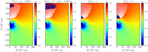
Figure 2: The $\nu_{e}-\bar{\nu}_{e}$ asymmetry parameter $\alpha$, defined as $\alpha=n_{\bar{\nu}_{e}}/n_{\nu_{e}}$, in the $t_{\rm{pb}}=200$ ms snapshot of the 2D SN model of an $11.2\mathrm{M}_{\odot}$ progenitor model [43]. White Crosses indicate the ELN crossings found in the data and the blue crosses are the ones which were captured by employing $\mathcal{F}(\mu)=(\mu-0.88)^{2}$, $-(\mu-1)^{3}$, $\mu$ and $\mu^{3}$, respectively. At this time, neutrinos decouple from matter at radius $\sim 50-70$ km depending on their flavors and energies.

In order to test our method, we pretended that we have access to only a few moments of the neutrino angular distribution instead of the full angular information, which was indeed provided by the Boltzmann calculations. Although the inequality proposed in Ref. [59] (which corresponds to employing $\mathcal{F}(\mu)=\mu^{2}\pm 2\mu+1$ ) can not capture any ELN crossings in this snapshot, one can capture a number of crossings by trying other quadratic $\mathcal{F}$’s (using only $I_{0}$, $I_{1}$ and $I_{2}$). For instance, in the first panel of Fig. 2, we show the ELN crossings which were captured by employing $\mathcal{F}(\mu)=(\mu-0.88)^{2}$ (blue crosses). These ELN crossings, which are $\gtrsim 5\%$ of the total number of ELN crossings in this snapshot, are located at relatively larger radii with $r\simeq 150-200$ km.

If $I_{3}$ is also available, a larger number of ELN crossings can be captured. For example, the ELN crossings captured by employing $\mathcal{F}(\mu)=(1-\mu)\times(\mu-0.88)^{2}$ are indicted in the second panel of Fig. 2. These crossings are located at $r\simeq 150-200$ km. By using $I_{3}$, we were able to capture approximately $\gtrsim 40\%$ of the total number of ELN crossings in this snapshot.

From these example, one can already observe that it is crucial to consider various forms of $\mathcal{F}(\mu)$ for having a good chance for capturing ELN crossings in the SN simulations. Otherwise, it is completely possible to miss a huge fraction (if not all) of the ELN crossings. In particular, the information available in higher moments, here $I_{3}$, is of utmost importance. This piece of information is totally useless in the method based on the instability of conversion modes, as can be clearly seen in Eq. (2.5).

In principle, the calculations that employ higher moments can capture larger number of ELN crossings. This simply comes from the fact that if $\mathcal{F}$ includes higher powers of $\mu$, it can better capture the details of the shape of ELN distribution. In order to have a better understanding of this, we considered a parametric ELN distribution of the from

$$G(\mu)=\left\{\begin{array}[]{ll}+1\quad\text{for}\quad\mu<1-\delta,\\ -h\quad\text{for}\quad\mu>1-\delta,\end{array}\right.$$ (2.7)

to mimic the shape of realistic ELN distributions (see, e.g., Fig. 5 in Ref. [44]). Such an ELN distribution has a crossing with the width of $\delta$ and the depth of $h$. As shown in Fig. 3, narrower crossings (smaller $\delta$’s) can be captured when higher angular moments are used, provided that they are deep (large $h$) enough. Although here the narrowest crossings can be captured when $I_{3}$ is used, calculations with only $I_{0}$ and $I_{1}$ can also capture some ELN crossings if they are wide and deep enough.

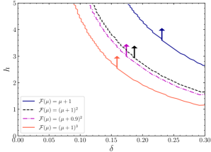
Figure 3: The curves above which ELN crossings can be captured for a number of $\mathcal{F}$’s and the ELN distribution defined in Eq. (2.7). Narrower (smaller $\delta$’s) and shallower (smaller $h$’s) ELN crossings can be captured when higher neutrino angular moments (higher powers of $\mu$) are employed.

Apart from $\mathcal{F}(\mu)$’s that are always positive in the interval $[-1,+1]$, one may also choose functions which are positive only within a certain range, however, provided that $G(\mu)$ is negligible within the range in which $\mathcal{F}(\mu)$ is not positive. In particular, one normally expects $G(\mu)$ to be almost negligible in the backward direction, i.e. for $\mu<0$, above the neutrinosphere. Thus, all $\mathcal{F}(\mu)$’s which are positive in the interval $[0,+1]$ could also be used for the SN zones above/within the decoupling region. However, it must be kept in mind that there is some uncertainty involved here because one needs to assume that $G(\mu)$ is small enough in the backward direction. ELN crossings captured by two such functions, namely $\mathcal{F}(\mu)=\mu$ and $\mathcal{F}(\mu)=\mu^{3}$ are shown in the right panels of Fig. 2, which are located at $r\simeq 60-90$ km. Here, we took the average radius of the neutrinosphere to be 60 km for this time snapshot.

The method we propose here focuses only on the occurrence of ELN crossings in the SN environment and does not aim at studying the unstable modes and their corresponding growth rates. Though having ELN crossing and fast modes are not necessarily equivalent from the mathematical point of view, they are most likely equivalent considering the expectations one has for the shape of the ELN distribution. In particular, one normally expects a single crossing  in $G(\mu)$ which means that the occurrence of fast modes and ELN crossings should be equivalent [34, 37]. In addition, because only a few moments are available, our method does (can) not capture extremely narrow crossings. This implies that the consequent growth rate of the unstable modes, $\kappa$, should be remarkably large, i.e. $\kappa\gtrsim(0.01-0.1)\mu$ [44].

Nevertheless, it might also be possible to make an estimate of the unstable modes and their growth rates by using a few neutrino angular moments. In particular, we observed that a parametric function with the form

$$\tilde{f}_{\nu}(\mu)\propto e^{-(1-\mu)^{\beta}/\alpha},$$ (2.8)

may appropriately capture neutrino and antineutrino angular distributions integrated over $E_{\nu}$ and $\phi_{\nu}$,

$$\tilde{f}_{\nu}(\mu)=\int_{0}^{\infty}\int_{0}^{2\pi}\frac{E_{\nu}^{2}\mathrm{d}E_{\nu}\mathrm{d}\phi_{\nu}}{(2\pi)^{3}}f_{\nu}(\mathbf{p}).$$ (2.9)

One can then calculate neutrino angular moments as a function of $\alpha$ and $\beta$ and use the moments available in the SN simulation to find the best fits for the parameters $\alpha$ and $\beta$ (for both $\nu_{e}$ and $\bar{\nu}_{e}$). In Fig. 4, we use the zeroth, first and second moments of neutrino angular distributions to find $\alpha$’s and $\beta$’s for $\nu_{e}$ and $\bar{\nu}_{e}$, and we plot the corresponding $G(\mu)$’s along with the ones obtained from the simulation of Ref. [44], at two different radii. Although we leave a dedicated and systematic study of the appropriateness of this fitting to a future work, it seems that the function proposed in Eq. (2.8) can be useful in capturing the overall shape of the ELN angular distribution and its potential crossings, though it could have its own limitations specifically at very large radii where the crossings get too narrow.

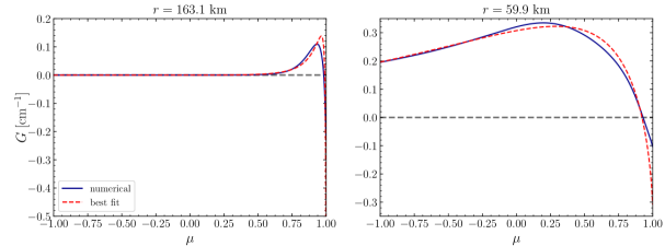
Figure 4: The best fits and numerical ELN angular distributions at two different radii. Eq. (2.8) can, indeed, provide a good estimate of the overall shape of the ELN angular distributions.

3 Conclusion

It is thought that neutrinos can undergo fast flavor conversions in dense neutrino media, such as those in CCSNe, provided that the angular distributions of the electron neutrino and antineutrino cross each other. Nevertheless, such detailed angular information is not available in most of the state-of-the-art CCSN simulations where instead, a few angular moments are considered in the treatment of the neutrino transport. We have proposed a new method to search for fast modes in such CCSN simulations. Our proposed method is based on the information in the available neutrino angular moments and it can use, and work with, as many angular moments as are provided by the SN simulation.

We check the practicability of our approach by employing it to some realistic neutrino angular distributions obtained from a 2D CCSN simulation. In particular, for the snapshot at $t_{\mathrm{pb}}=200$ ms, we show that it can capture $\gtrsim 40\%$ of the total number of ELN crossings when $I_{0}$, $I_{1}$, $I_{2}$ and $I_{3}$ are all available. This should be compared with the methods based on the instability of the zeroth mode [59] which can not capture any crossing in this snapshot. This indicates the high efficiency of our proposed method to extract the most available information in the neutrino angular moments. We show that this is not coincidental and indeed, can be understood by considering the shape of the ELN distributions expected in the neutrino decoupling region.

Although the occurrence of the ELN crossings is most likely a necessary condition for fast modes, it may not, in general, be a sufficient condition. However, for a physically reasonable ELN angular distribution, it can be also a sufficient condition [34, 37]. In addition, since CCSN simulations consider only a few neutrino angular moments, our method is not aggressive in terms of distinguishing very narrow crossings. Hence, any crossings captured by our method can be expected to result in fast flavor conversion modes with significant growth rates.

While we have utilized our method to capture the crossings in the $\phi_{\nu}$-integrated ELN distribution, it can be also used to capture the crossings which may occur in $\phi_{\nu}$. To achieve this goal, one just need to modify Eq. (2.1) to

$$I_{\mathcal{F}}=\int_{-1}^{1}\int_{0}^{2\pi}\mathrm{d}\mu\mathrm{d}\phi_{\nu}\ \mathcal{F}(\mu,\phi_{\nu})\ \tilde{G}_{\rm{\bf{v}}},$$ (3.1)

where

$$\tilde{G}_{\rm{\bf{v}}}=\sqrt{2}G_{\mathrm{F}}\int_{0}^{\infty}\frac{E_{\nu}^{2}\mathrm{d}E_{\nu}}{(2\pi)^{3}}[f_{\nu_{e}}(\mathbf{p})-f_{\bar{\nu}_{e}}(\mathbf{p})],$$ (3.2)

and $\mathcal{F}(\mu,\phi_{\nu})$ is a positive function of $\mu$ and $\phi_{\nu}$. For example, in the $M_{1}$ neutrino transport scheme, one can choose $\mathcal{F}(\mu,\phi_{\nu})=\mu^{2}\cos^{2}\phi_{\nu}$ and so on.

In this study, we also propose a parametric function that could appropriately describe neutrino and antineutrino angular distributions. This way, one can also study the unstable modes in the neutrino gas and make an estimate of their fast growth rates.

Fast modes can also appear in neutron star mergers (NSM) [30] where the neutrino gas can be extremely dense. The method proposed here is not limited to the case of CCSN simulations and can be also used in NSM simulations where the neutrino transport is treated by moments method [62].

Despite the fact that a number of studies have detected fast modes in CCSN simulations, a comprehensive understanding of the characteristics of the fast modes in 3D SN models is still missing. Our study allows for a more efficient identification of the ELN crossings in the SN/NSM environments and can lead to improvement of our understanding of the neutrino flavor evolution in such astrophysical settings.

References

- [1] S. A. Colgate, R. H. White, The Hydrodynamic Behavior of Supernovae Explosions, Astrophys. J. 143 (1966) 626. doi:10.1086/148549.
- [2] H. A. Bethe, J. R. Wilson, Revival of a stalled supernova shock by neutrino heating, Astrophys. J. 295 (1985) 14–23. doi:10.1086/163343.
- [3] H.-T. Janka, Explosion Mechanisms of Core-Collapse Supernovae, Ann. Rev. Nucl. Part. Sci. 62 (2012) 407–451. arXiv:1206.2503, doi:10.1146/annurev-nucl-102711-094901.
- [4] A. Burrows, Colloquium: Perspectives on core-collapse supernova theory, Rev. Mod. Phys. 85 (2013) 245. arXiv:1210.4921, doi:10.1103/RevModPhys.85.245.
- [5] S. Pastor, G. Raffelt, Flavor oscillations in the supernova hot bubble region: Nonlinear effects of neutrino background, Phys. Rev. Lett. 89 (2002) 191101. arXiv:astro-ph/0207281.
- [6] H. Duan, G. M. Fuller, J. Carlson, Y.-Z. Qian, Simulation of Coherent Non-Linear Neutrino Flavor Transformation in the Supernova Environment. 1. Correlated Neutrino Trajectories, Phys. Rev. D74 (2006) 105014. arXiv:astro-ph/0606616, doi:10.1103/PhysRevD.74.105014.
- [7] H. Duan, G. M. Fuller, J. Carlson, Y.-Z. Qian, Coherent Development of Neutrino Flavor in the Supernova Environment, Phys. Rev. Lett. 97 (2006) 241101. arXiv:astro-ph/0608050, doi:10.1103/PhysRevLett.97.241101.
- [8] H. Duan, G. M. Fuller, Y.-Z. Qian, Collective Neutrino Oscillations, Ann. Rev. Nucl. Part. Sci. 60 (2010) 569–594. arXiv:1001.2799, doi:10.1146/annurev.nucl.012809.104524.
- [9] S. Chakraborty, R. Hansen, I. Izaguirre, G. Raffelt, Collective neutrino flavor conversion: Recent developments, Nucl. Phys. B908 (2016) 366–381. arXiv:1602.02766, doi:10.1016/j.nuclphysb.2016.02.012.
- [10] Y. Z. Qian, S. E. Woosley, Nucleosynthesis in neutrino driven winds: 1. The Physical conditions, Astrophys. J. 471 (1996) 331–351. arXiv:astro-ph/9611094, doi:10.1086/177973.
- [11] H. Duan, G. M. Fuller, J. Carlson, Y.-Z. Qian, Flavor Evolution of the Neutronization Neutrino Burst from an O-Ne-Mg Core-Collapse Supernova, Phys. Rev. Lett. 100 (2008) 021101. arXiv:0710.1271, doi:10.1103/PhysRevLett.100.021101.
- [12] B. Dasgupta, A. Dighe, G. G. Raffelt, A. Y. Smirnov, Multiple Spectral Splits of Supernova Neutrinos, Phys. Rev. Lett. 103 (2009) 051105. arXiv:0904.3542, doi:10.1103/PhysRevLett.103.051105.
- [13] S. Galais, C. Volpe, The neutrino spectral split in core-collapse supernovae: a magnetic resonance phenomenon, Phys. Rev. D84 (2011) 085005. arXiv:1103.5302, doi:10.1103/PhysRevD.84.085005.
- [14] H. Duan, G. M. Fuller, J. Carlson, Y.-Z. Qian, Neutrino Mass Hierarchy and Stepwise Spectral Swapping of Supernova Neutrino Flavors, Phys. Rev. Lett. 99 (2007) 241802. arXiv:0707.0290, doi:10.1103/PhysRevLett.99.241802.
- [15] H. Duan, Collective neutrino oscillations and spontaneous symmetry breaking, Int. J. Mod. Phys. E24 (09) (2015) 1541008. arXiv:1506.08629, doi:10.1142/S0218301315410086.
- [16] G. Raffelt, S. Sarikas, D. d. S. Seixas, Axial symmetry breaking in self-induced flavor conversion of supernova neutrino fluxes, Phys. Rev. Lett. 111 (2013) 091101. arXiv:1305.7140, doi:10.1103/PhysRevLett.111.091101.
- [17] H. Duan, Flavor Oscillation Modes In Dense Neutrino Media, Phys. Rev. D88 (2013) 125008. arXiv:1309.7377, doi:10.1103/PhysRevD.88.125008.
- [18] H. Duan, S. Shalgar, Flavor instabilities in the neutrino line model, Phys. Lett. B747 (2015) 139–143. arXiv:1412.7097, doi:10.1016/j.physletb.2015.05.057.
- [19] S. Abbar, H. Duan, S. Shalgar, Flavor instabilities in the multiangle neutrino line model, Phys. Rev. D92 (6) (2015) 065019. arXiv:1507.08992, doi:10.1103/PhysRevD.92.065019.
- [20] S. Abbar, H. Duan, Neutrino flavor instabilities in a time-dependent supernova model, Phys. Lett. B751 (2015) 43–47. arXiv:1509.01538, doi:10.1016/j.physletb.2015.10.019.
- [21] S. Chakraborty, R. S. Hansen, I. Izaguirre, G. Raffelt, Self-induced flavor conversion of supernova neutrinos on small scales, JCAP 1601 (01) (2016) 028. arXiv:1507.07569, doi:10.1088/1475-7516/2016/01/028.
- [22] B. Dasgupta, A. Mirizzi, Temporal Instability Enables Neutrino Flavor Conversions Deep Inside Supernovae, Phys. Rev. D92 (12) (2015) 125030. arXiv:1509.03171, doi:10.1103/PhysRevD.92.125030.
- [23] A. Mirizzi, G. Mangano, N. Saviano, Self-induced flavor instabilities of a dense neutrino stream in a two-dimensional model, Phys. Rev. D92 (2) (2015) 021702. arXiv:1503.03485, doi:10.1103/PhysRevD.92.021702.
- [24] J. D. Martin, C. Yi, H. Duan, Dynamic fast flavor oscillation waves in dense neutrino gases, Phys. Lett. B800 (2020) 135088. arXiv:1909.05225, doi:10.1016/j.physletb.2019.135088.
- [25] J. D. Martin, S. Abbar, H. Duan, Nonlinear flavor development of a two-dimensional neutrino gas, Phys. Rev. D100 (2) (2019) 023016. arXiv:1904.08877, doi:10.1103/PhysRevD.100.023016.
- [26] R. F. Sawyer, Speed-up of neutrino transformations in a supernova environment, Phys. Rev. D72 (2005) 045003. arXiv:hep-ph/0503013, doi:10.1103/PhysRevD.72.045003.
- [27] R. F. Sawyer, Neutrino cloud instabilities just above the neutrino sphere of a supernova, Phys. Rev. Lett. 116 (8) (2016) 081101. arXiv:1509.03323, doi:10.1103/PhysRevLett.116.081101.
- [28] S. Chakraborty, R. S. Hansen, I. Izaguirre, G. Raffelt, Self-induced neutrino flavor conversion without flavor mixing, JCAP 1603 (03) (2016) 042. arXiv:1602.00698, doi:10.1088/1475-7516/2016/03/042.
- [29] I. Izaguirre, G. Raffelt, I. Tamborra, Fast Pairwise Conversion of Supernova Neutrinos: A Dispersion-Relation Approach, Phys. Rev. Lett. 118 (2) (2017) 021101. arXiv:1610.01612, doi:10.1103/PhysRevLett.118.021101.
- [30] M.-R. Wu, I. Tamborra, Fast neutrino conversions: Ubiquitous in compact binary merger remnants, Phys. Rev. D95 (10) (2017) 103007. arXiv:1701.06580, doi:10.1103/PhysRevD.95.103007.
- [31] F. Capozzi, B. Dasgupta, E. Lisi, A. Marrone, A. Mirizzi, Fast flavor conversions of supernova neutrinos: Classifying instabilities via dispersion relations, Phys. Rev. D96 (4) (2017) 043016. arXiv:1706.03360, doi:10.1103/PhysRevD.96.043016.
- [32] S. A. Richers, G. C. McLaughlin, J. P. Kneller, A. Vlasenko, Neutrino Quantum Kinetics in Compact Objects, Phys. Rev. D99 (12) (2019) 123014. arXiv:1903.00022, doi:10.1103/PhysRevD.99.123014.
- [33] B. Dasgupta, A. Mirizzi, M. Sen, Fast neutrino flavor conversions near the supernova core with realistic flavor-dependent angular distributions, JCAP 1702 (02) (2017) 019. arXiv:1609.00528, doi:10.1088/1475-7516/2017/02/019.
- [34] S. Abbar, H. Duan, Fast neutrino flavor conversion: roles of dense matter and spectrum crossing, Phys. Rev. D98 (4) (2018) 043014. arXiv:1712.07013, doi:10.1103/PhysRevD.98.043014.
- [35] S. Abbar, M. C. Volpe, On Fast Neutrino Flavor Conversion Modes in the Nonlinear Regime, Phys. Lett. B790 (2019) 545–550. arXiv:1811.04215, doi:10.1016/j.physletb.2019.02.002.
- [36] F. Capozzi, B. Dasgupta, A. Mirizzi, M. Sen, G. Sigl, Collisional triggering of fast flavor conversions of supernova neutrinos, Phys. Rev. Lett. 122 (9) (2019) 091101. arXiv:1808.06618, doi:10.1103/PhysRevLett.122.091101.
- [37] F. Capozzi, G. Raffelt, T. Stirner, Fast Neutrino Flavor Conversion: Collective Motion vs. Decoherence, JCAP 1909 (2019) 002. arXiv:1906.08794, doi:10.1088/1475-7516/2019/09/002.
- [38] C. Döring, R. S. L. Hansen, M. Lindner, Stability of three neutrino flavor conversion in supernovae, JCAP 1908 (2019) 003. arXiv:1905.03647, doi:10.1088/1475-7516/2019/08/003.
- [39] M. Chakraborty, S. Chakraborty, Three flavor neutrino conversions in supernovae: Slow Fast instabilitiesarXiv:1909.10420.
- [40] L. Johns, H. Nagakura, G. M. Fuller, A. Burrows, Neutrino oscillations in supernovae: angular moments and fast instabilitiesarXiv:1910.05682.
- [41] S. Shalgar, I. Padilla-Gay, I. Tamborra, Neutrino propagation hinders fast pairwise flavor conversionsarXiv:1911.09110.
- [42] J. F. Cherry, G. M. Fuller, S. Horiuchi, K. Kotake, T. Takiwaki, T. Fischer, Time of Flight and Supernova Progenitor Effects on the Neutrino HaloarXiv:1912.11489.
- [43] S. Abbar, H. Duan, K. Sumiyoshi, T. Takiwaki, M. C. Volpe, On the occurrence of fast neutrino flavor conversions in multidimensional supernova models, Phys. Rev. D100 (4) (2019) 043004. arXiv:1812.06883, doi:10.1103/PhysRevD.100.043004.
- [44] S. Abbar, H. Duan, K. Sumiyoshi, T. Takiwaki, M. C. Volpe, Fast Neutrino Flavor Conversion Modes in Multidimensional Core-collapse Supernova Models: the Role of the Asymmetric Neutrino DistributionsarXiv:1911.01983.
- [45] M. Delfan Azari, S. Yamada, T. Morinaga, H. Nagakura, S. Furusawa, A. Harada, H. Okawa, W. Iwakami, K. Sumiyoshi, Fast collective neutrino oscillations inside the neutrino sphere in core-collapse supernovaearXiv:1910.06176.
- [46] H. Nagakura, T. Morinaga, C. Kato, S. Yamada, Fast-pairwise collective neutrino oscillations associated with asymmetric neutrino emissions in core-collapse supernovaarXiv:1910.04288.
- [47] T. Morinaga, H. Nagakura, C. Kato, S. Yamada, A new possibility of the fast neutrino-flavor conversion in the pre-shock region of core-collapse supernovaarXiv:1909.13131.
- [48] R. Glas, H. T. Janka, F. Capozzi, M. Sen, B. Dasgupta, A. Mirizzi, G. Sigl, Fast Neutrino Flavor Instability in the Neutron-star Convection Layer of Three-dimensional Supernova ModelsarXiv:1912.00274.
- [49] M. Rampp, H. T. Janka, Radiation hydrodynamics with neutrinos: Variable Eddington factor method for core collapse supernova simulations, Astron. Astrophys. 396 (2002) 361. arXiv:astro-ph/0203101, doi:10.1051/0004-6361:20021398.
- [50] I. Tamborra, F. Hanke, H.-T. Janka, B. Müller, G. G. Raffelt, A. Marek, Self-sustained asymmetry of lepton-number emission: A new phenomenon during the supernova shock-accretion phase in three dimensions, Astrophys. J. 792 (2) (2014) 96. arXiv:1402.5418, doi:10.1088/0004-637X/792/2/96.
- [51] S. W. Bruenn, et al., The Development of Explosions in Axisymmetric AB INITIO Core-Collapse Supernova Simulations of 12-25 Stars, Astrophys. J. 818 (2) (2016) 123. arXiv:1409.5779, doi:10.3847/0004-637X/818/2/123.
- [52] E. P. O’Connor, S. M. Couch, Two Dimensional Core-Collapse Supernova Explosions Aided by General Relativity with Multidimensional Neutrino Transport, Astrophys. J. 854 (1) (2018) 63. arXiv:1511.07443, doi:10.3847/1538-4357/aaa893.
- [53] S. Richers, H. Nagakura, C. D. Ott, J. Dolence, K. Sumiyoshi, S. Yamada, A Detailed Comparison of Multidimensional Boltzmann Neutrino Transport Methods in Core-collapse Supernovae, Astrophys. J. 847 (2) (2017) 133. arXiv:1706.06187, doi:10.3847/1538-4357/aa8bb2.
- [54] D. Vartanyan, A. Burrows, D. Radice, M. A. Skinner, J. Dolence, Revival of the Fittest: Exploding Core-Collapse Supernovae from 12 to 25 M⊙, Mon. Not. Roy. Astron. Soc. 477 (3) (2018) 3091–3108. arXiv:1801.08148, doi:10.1093/mnras/sty809.
- [55] O. Just, R. Bollig, H.-T. Janka, M. Obergaulinger, R. Glas, S. Nagataki, Core-collapse supernova simulations in one and two dimensions: comparison of codes and approximations, Mon. Not. Roy. Astron. Soc. 481 (4) (2018) 4786–4814. arXiv:1805.03953, doi:10.1093/mnras/sty2578.
- [56] K.-C. Pan, C. Mattes, E. P. O’Connor, S. M. Couch, A. Perego, A. Arcones, The Impact of Different Neutrino Transport Methods on Multidimensional Core-collapse Supernova Simulations, J. Phys. G46 (1) (2019) 014001. arXiv:1806.10030, doi:10.1088/1361-6471/aaed51.
- [57] O. Just, M. Obergaulinger, H. T. Janka, A new multidimensional, energy-dependent two-moment transport code for neutrino-hydrodynamics, Mon. Not. Roy. Astron. Soc. 453 (4) (2015) 3386–3413. arXiv:1501.02999, doi:10.1093/mnras/stv1892.
- [58] L. M. Murchikova, E. Abdikamalov, T. Urbatsch, Analytic Closures for M1 Neutrino Transport, Mon. Not. Roy. Astron. Soc. 469 (2) (2017) 1725–1737. arXiv:1701.07027, doi:10.1093/mnras/stx986.
- [59] B. Dasgupta, A. Mirizzi, M. Sen, Simple method of diagnosing fast flavor conversions of supernova neutrinos, Phys. Rev. D98 (10) (2018) 103001. arXiv:1807.03322, doi:10.1103/PhysRevD.98.103001.
- [60] K. Sumiyoshi, S. Yamada, Neutrino Transfer in Three Dimensions for Core-Collapse Supernovae. I. Static Configurations, Astrophys. J. Suppl. 199 (2012) 17. arXiv:1201.2244, doi:10.1088/0067-0049/199/1/17.
- [61] K. Sumiyoshi, T. Takiwaki, H. Matsufuru, S. Yamada, Multi-dimensional Features of Neutrino Transfer in Core-Collapse Supernovae, Astrophys. J. Suppl. 216 (2015) 5. arXiv:1403.4476, doi:10.1088/0067-0049/216/1/5.
- [62] O. Just, A. Bauswein, R. A. Pulpillo, S. Goriely, H. T. Janka, Comprehensive nucleosynthesis analysis for ejecta of compact binary mergers, Mon. Not. Roy. Astron. Soc. 448 (1) (2015) 541–567. arXiv:1406.2687, doi:10.1093/mnras/stv009.