Structured Prediction with Partial Labelling through the Infimum Loss

Abstract

Annotating datasets is one of the main costs in nowadays supervised learning. The goal of weak supervision is to enable models to learn using only forms of labelling which are cheaper to collect, as partial labelling. This is a type of incomplete annotation where, for each datapoint, supervision is cast as a set of labels containing the real one. The problem of supervised learning with partial labelling has been studied for specific instances such as classification, multi-label, ranking or segmentation, but a general framework is still missing. This paper provides a unified framework based on structured prediction and on the concept of infimum loss to deal with partial labelling over a wide family of learning problems and loss functions. The framework leads naturally to explicit algorithms that can be easily implemented and for which proved statistical consistency and learning rates. Experiments confirm the superiority of the proposed approach over commonly used baselines.

appendixAppendix References

1 Introduction

Fully supervised learning demands tight supervision of large amounts of data, a supervision that can be quite costly to acquire and constrains the scope of applications. To overcome this bottleneck, the machine learning community is seeking to incorporate weaker sources of information in the learning framework. In this paper, we address those limitations through partial labelling: e.g., giving only partial ordering when learning user preferences over items, or providing the label “flower" for a picture of Arum Lilies, instead of spending a consequent amount of time to find the exact taxonomy.

Partial labelling has been studied in the context of classification (Cour et al., 2011; Nguyen & Caruana, 2008), multilabelling (Yu et al., 2014), ranking (Hüllermeier et al., 2008; Korba et al., 2018), as well as segmentation (Verbeek & Triggs, 2008; Papandreou et al., 2015), or natural language processing tasks (Fernandes & Brefeld, 2011; Mayhew et al., 2019), however a generic framework is still missing. Such a framework is a crucial step towards understanding how to learn from weaker sources of information, and widening the spectrum of machine learning beyond rigid applications of supervised learning. Some interesting directions are provided by Cid-Sueiro et al. (2014); van Rooyen & Williamson (2017), to recover the information lost in a corrupt acquisition of labels. Yet, they assume that the corruption process is known, which is a strong requirement that we want to relax.

In this paper, we make the following contributions:

• We provide a principled framework to solve the problem of learning with partial labelling, via structured prediction. This approach naturally leads to a variational framework built on the infimum loss.

• We prove that the proposed framework is able to recover the original solution of the supervised learning problem under identifiability assumptions on the labelling process.

• We derive an explicit algorithm which is easy to train and with strong theoretical guarantees. In particular, we prove that it is consistent and we provide generalization error rates.

• Finally, we test our method against some simple baselines, on synthetic and real examples. We show that for certain partial labelling scenarios with symmetries, our infimum loss performs similarly to a simple baseline. However in scenarios where the acquisition process of the labels is more adversarial in nature, the proposed algorithm performs consistently better.

2 Partial labelling with infimum loss

In this section, we introduce a statistical framework for partial labelling, and we show that it is characterized naturally in terms of risk minimization with the infimum loss. First, let’s recall some elements of fully supervised and weakly supervised learning.

Fully supervised learning consists in learning a function ${f\in\mathcal{Y}^{\mathcal{X}}}$ between a input space $\mathcal{X}$ and a output space $\mathcal{Y}$, given a joint distribution ${\rho\in\Delta_{\mathcal{X}\times\mathcal{Y}}}$ on ${\mathcal{X}\times\mathcal{Y}}$, and a loss function ${\ell\in\mathbb{R}^{\mathcal{Y}\times\mathcal{Y}}}$, that minimizes the risk

$${\cal R}(f;\rho)=\operatorname{\mathbb{E}}_{(X,Y)\sim\rho}\left[\ell(f(X),Y)\right],$$ (1)

given observations ${(x_{i},y_{i})_{i\leq n}\sim\rho^{\otimes n}}$. We will assume that the loss $\ell$ is proper, i.e. it is continuous non-negative and is zero on, and only on, the diagonal of ${\mathcal{Y}\times\mathcal{Y}}$, and strictly positive outside. We will also assume that $\mathcal{Y}$ is compact.

In weakly supervised learning, given $(x_{i})_{i\leq n}$, one does not have direct observations of $(y_{i})_{i\leq n}$ but weaker information. The goal is still to recover the solution ${f\in\mathcal{Y}^{\mathcal{X}}}$ of the fully supervised problem Eq. 1. In partial labelling, also known as superset learning or as learning with ambiguous labels, which is an instance of weak supervision, information is cast as closed sets $(S_{i})_{i\leq n}$ in ${\cal S}$, where ${\cal S}\subset 2^{\mathcal{Y}}$ is the space of closed subsets of $\mathcal{Y}$, containing the true labels ${(y_{i}\in S_{i})}$. In this paper, we model this scenario by considering a data distribution ${\tau\in\Delta_{\mathcal{X}\times{\cal S}}}$, that generates the samples $(x_{i},S_{i})$. We will denote $\tau$ as weak distribution to distinguish it from $\rho$. Capturing the dependence on the original problem, $\tau$ must be compatible with $\rho$, a matching property that we formalize with the concept of eligibility.

Definition 1 (Eligibility).

Given a probability measure $\tau$ on $\mathcal{X}\times{\cal S}$, a probability measure $\rho$ on $\mathcal{X}\times\mathcal{Y}$ is said to be eligible for $\tau$ (denoted by $\rho\vdash\tau$), if there exists a probability measure $\pi$ over $\mathcal{X}\times\mathcal{Y}\times{\cal S}$ such that $\rho$ is the marginal of $\pi$ over $\mathcal{X}\times\mathcal{Y}$, $\tau$ is the marginal of $\pi$ over $\mathcal{X}\times{\cal S}$, and, for $y\in\mathcal{Y}$ and $S\in{\cal S}$

$$y\notin S\qquad\Rightarrow\qquad\operatorname{\mathbb{P}}_{\pi}\left(S\,\middle|\,Y=y\right)=0.$$

We will alternatively say that $\tau$ is a weakening of $\rho$, or that $\rho$ and $\tau$ are compatible.

2.1 Disambiguation principle

According to the setting described above, the problem of partial labelling is completely defined by a loss and a weak distribution $(\ell,\tau)$. The goal is to recover the solution of the original supervised learning problem in Eq. 1 assuming that the original distribution verifies $\rho\vdash\tau$. Since more than one $\rho$ may be eligible for $\tau$, we would like to introduce a guiding principle to identify a $\rho^{\star}$ among them. With this goal we define the concept of non-ambiguity for $\tau$, a setting in which a natural choice for $\rho^{\star}$ appears.

Definition 2 (Non-ambiguity).

For any $x\in\mathcal{X}$, denote by $\tau|_{x}$ the conditional probability of $\tau$ given $x$, and define the set $S_{x}$ as

$$S_{x}=\bigcap_{S\in\operatorname*{supp}(\tau|_{x})}S.$$

The weak distribution $\tau$ is said non-ambiguous if, for every $x\in\mathcal{X}$, $S_{x}$ is a singleton. Moreover, we say that $\tau$ is strictly non-ambiguous if it is non-ambiguous and there exists ${\eta\in(0,1)}$ such that, for all ${x\in\mathcal{X}}$ and ${z\notin S_{x}}$

$$\operatorname{\mathbb{P}}_{S\sim\tau|_{x}}(z\in S)\leq 1-\eta.$$

This concept is similar to the one by Cour et al. (2011), but more subtle because this quantity only depends on $\tau$, and makes no assumption on the original distribution $\rho$ describing the fully supervised process that we can not access. In this sense, it is also more general.

When $\tau$ is non-ambiguous, we can write $S_{x}=\left\{y_{x}\right\}$ for any $x$, where $y_{x}$ is the only element of $S_{x}$. In this case it is natural to identify $\rho^{\star}$ as the one satisfying $\rho^{\star}|_{x}=\delta_{y_{x}}$. Actually, such a $\rho^{\star}$ is characterized without $S_{x}$ as the only deterministic distribution that is eligible for $\tau$. Because deterministic distributions are characterized as minimizing the minimum risk of Eq. 1, we introduce the following minimum variability principle to disambiguate between all eligible $\rho$’s, and identify $\rho^{\star}$,

$$\rho^{\star}\in\operatorname*{arg\,min}_{\rho\vdash\tau}{\cal E}(\rho),\qquad{\cal E}(\rho)=\inf_{f:\mathcal{X}\to\mathcal{Y}}{\cal R}(f;\rho).$$ (2)

The quantity ${\cal E}$ can be identified as a variance, since if $f_{\rho}$ is the minimizer of ${\cal R}(f;\rho)$, $f_{\rho}(x)$ can be seen as the mean of $\rho|_{x}$ and $\ell$ the natural distance in $\mathcal{Y}$. Indeed, when $\ell=\ell_{2}$ is the mean square loss, this is exactly the case. The principle above recovers exactly $\rho^{\star}|_{x}=\delta_{y_{x}}$, when $\tau$ is non-ambiguous, as stated by Prop. 1, proven in Sec. A.1.

Proposition 1 (Non-ambiguity determinism).

When $\tau$ is non-ambiguous, the solution $\rho^{\star}$ of Eq. 2 exists and satisfies that, for any $x\in\mathcal{X}$, $\rho^{\star}|_{x}=\delta_{y_{x}}$, where $y_{x}$ is the only element of $S_{x}$.

Prop. 1 provides a justification for the usage of the minimum variability principle. Indeed, under non-ambiguity assumption, following this principle will allow us to build an algorithm that recover the original fully supervised distribution. Therefore, given samples $(x_{i},S_{i})$, it is of interest to test if $\tau$ is non-ambiguous. Such tests should leverage other regularity hypothesis on $\tau$, which we will not address in this work.

Now, we characterize the minimum variability principle in terms of a variational optimization problem that we can tackle in Sec. 3 via empirical risk minimization.

2.2 Variational formulation via the infimum loss

Given a partial labelling problem $(\ell,\tau)$, define the solutions based on the minimum variablity principle as the functions minimizing the recovered risk

$$f^{*}\in\operatorname*{arg\,min}_{f:\mathcal{X}\to\mathcal{Y}}{\cal R}(f;\rho^{\star}).$$ (3)

for $\rho^{\star}$ a distribution solving Eq. 2. As shown in Thm. 1 below, proven in Sec. A.2, the proposed disambiguation paradigm naturally leads to a variational framework involving the infimum loss.

Theorem 1 (Infimum loss (IL)).

The functions $f^{*}$ defined in Eq. 3 are characterized as

$$f^{*}\in\operatorname*{arg\,min}_{f:\mathcal{X}\to\mathcal{Y}}{\cal R}_{S}(f),$$

where the risk ${\cal R}_{S}$ is defined as

$${\cal R}_{S}(f)=\operatorname{\mathbb{E}}_{(X,S)\sim\tau}\left[L(f(X),S)\right],$$ (4)

and $L$ is the infimum loss

$$L(z,S)=\inf_{y\in S}\ell(z,y).$$ (5)

The infimum loss, also known as the ambiguous loss (Luo & Orabona, 2010; Cour et al., 2011), or as the optimistic superset loss (Hüllermeier, 2014), captures the idea that, when given a set $S$, this set contains the good label $y$ but also a lot of bad ones, that should not be taken into account when retrieving $f$. In other terms, $f$ should only match the best guess in $S$. Indeed, if $\ell$ is seen as a distance, $L$ is its natural extension to sets.

2.3 Recovery of the fully supervised solutions

In this subsection, we investigate the setting where an original fully supervised learning problem $\rho_{0}$ has been weakened due to incomplete labelling, leading to a weak distribution $\tau$. The goal here is to understand under which conditions on $\tau$ and $\ell$ it is possible to recover the original fully supervised solution based with the infimum loss framework. Denote $f_{0}$ the function minimizing ${\cal R}(f;\rho_{0})$. The theorem below, proven in Sec. A.3, shows that under non-ambiguity and deterministic conditions, it is possible to fully recover the function $f_{0}$ also from $\tau$.

Theorem 2 (Supervision recovery).

For an instance $(\ell,\rho_{0},\tau)$ of the weakened supervised problem, if we denote by $f_{0}$ the minimizer of Eq. 1, we have the under the conditions that (1) $\tau$ is not ambiguous (2) for all $x\in\mathcal{X}$, $S_{x}=\left\{f_{0}(x)\right\}$; the infimum loss recovers the original fully supervised solution, i.e. the $f^{*}$ defined in Eq. 3 verifies $f^{*}=f_{0}$.

Futhermore, when $\rho_{0}$ is deterministic and $\tau$ not ambiguous, the $\rho^{\star}$ defined in Eq. 2 verifies $\rho^{\star}=\rho_{0}$.

At a comprehensive levels, this theorem states that under non-ambiguity of the partial labelling process, if the labels are a deterministic function of the inputs, the infimum loss framework make it possible to recover the solution of the original fully supervised problem while only accessing weak labels. In the next subsection, we will investigate which is the relation between the two problems when dealing with an estimator $f$ of $f^{*}$.

2.4 Comparison inequality

In the following, we want to characterize the error performed by ${\cal R}(f;\rho^{\star})$ with respect to the error performed by ${\cal R}_{S}(f)$. This will be useful since, in the next section, we will provide an estimator for $f^{*}$ based on structured prediction, that minimize the risk ${\cal R}_{S}$. First, we introduce a measure of discrepancy for the loss function.

Definition 3 (Discrepancy of the loss $\ell$).

Given a loss function $\ell$, the discrepancy degree $\nu$ of $\ell$ is defined as

$$\nu=\log\sup_{y,z^{\prime}\neq z}\frac{\ell(z,y)}{\ell(z,z^{\prime})}.$$

$\mathcal{Y}$ will be said discrete for $\ell$ when $\nu<+\infty$, which is always the case when $\mathcal{Y}$ is finite.

Now we are ready to state the comparison inequality that generalizes to arbitrary losses and output spaces a result on $0-1$ loss on classification from Cour et al. (2011).

Proposition 2 (Comparison inequality).

When $\mathcal{Y}$ is discrete and $\tau$ is strictly non-ambiguous for a given $\eta\in(0,1)$, then the following holds

$${\cal R}(f;\rho^{\star})-{\cal R}(f^{*};\rho^{\star})\leq C({\cal R}_{S}(f)-{\cal R}_{S}(f^{*})),$$ (6)

for any measurable function $f\in\mathcal{Y}^{\mathcal{X}}$, where $C$ does not depend on $\tau,f$, and is defined as follows and always finite

$$C=\eta^{-1}e^{\nu}.$$

When $\rho_{0}$ is deterministic, since we know from Thm. 2 that $\rho^{\star}=\rho_{0}$, this theorem allows to bound the error made on the original fully supervised problem with the error measured with the infimum loss on the weakly supervised one.

Note that the constant presented above is the product of two independent terms, the first measuring the ambiguity of the weak distribution $\tau$, and the second measuring a form of discrepancy for the loss. In the appendix, we provide a more refined bound for $C$, that is $C=C(\ell,\tau)$, that shows a more elaborated interaction between $\ell$ and $\tau$. This may be interesting in situations where it is possible to control the labelling process and may suggest strategies to active partial labelling, with the goal of minimizing the costs of labelling while preserving the properties presented in this section and reducing the impact of the constant $C$ in the learning process. An example is provided in the Sec. A.5.

3 Consistent algorithm for partial labelling

In this section, we provide an algorithmic approach based on structured prediction to solve the weak supervised learning problem expressed in terms of infimum loss from Thm. 1. From this viewpoint, we could consider different structured prediction frameworks as structured SVM (Tsochantaridis et al., 2005), conditional random fields (Lafferty et al., 2001) or surrogate mean estimation (Ciliberto et al., 2016). For example, Luo & Orabona (2010) used a margin maximization formulation in a structured SVM fashion, Hüllermeier & Cheng (2015) went for nearest neighbors, and Cour et al. (2011) design a surrogate method specific to the 0-1 loss, for which they show consistency based on Bartlett et al. (2006).

In the following, we will use the structured prediction method of Ciliberto et al. (2016); Nowak-Vila et al. (2019), which allows us to derive an explicit estimator, easy to train and with strong theoretical properties, in particular, consistency and finite sample bounds for the generalization error. The estimator is based on the pointwise characterization of $f^{*}$ as

$$f^{*}(x)\in\operatorname*{arg\,min}_{z\in\mathcal{Y}}\operatorname{\mathbb{E}}_{S\sim\tau|_{x}}\left[\inf_{y\in S}\ell(z,y)\right],$$

and weights $\alpha_{i}(x)$ that are trained on the dataset such that $\hat{\tau}_{|x}=\sum_{i=1}^{n}\alpha_{i}(x)\delta_{S_{i}}$ is a good approximation of $\tau|_{x}$. Plugging this approximation in the precedent equation leads to our estimator, that is defined explicity as follows

$$f_{n}(x)\in\operatorname*{arg\,min}_{z\in\mathcal{Y}}\inf_{y_{i}\in S_{i}}\sum_{i=1}^{n}\alpha_{i}(x)\ell(z,y_{i}).$$ (7)

Among possible choices for $\alpha$, we will consider the following kernel ridge regression estimator to be learned at training time

$$\alpha(x)=(K+n\lambda)^{-1}v(x),$$

with $\lambda>0$ a regularizer parameter and $K=(k(x_{i},x_{j}))_{i,j}\in\mathbb{R}^{n\times n},v(x)=(k(x,x_{i}))_{i}\in\mathbb{R}^{n}$ where $k\in\mathcal{X}\times\mathcal{X}\to\mathbb{R}$ is a positive-definite kernel (Scholkopf & Smola, 2001) that defines a similarity function between input points (e.g., if $\mathcal{X}=\mathbb{R}^{d}$ for some $d\in\mathbb{N}$ a commonly used kernel is the Gaussian kernel $k(x,x^{\prime})=e^{-\|x-x^{\prime}\|^{2}}$). Other choices can be done to learn $\alpha$, beyond kernel methods, a particularly appealing one is harmonic functions, incorporating a prior on low density separation to boost learning (Zhu et al., 2003; Zhou et al., 2003; Bengio et al., 2006). Here we use the kernel estimator since it allows to derive strong theoretical results, based on kernel conditional mean estimation (Muandet et al., 2017).

3.1 Theoretical guarantees

In this following, we want to prove that $f_{n}$ converges to $f^{*}$ as $n$ goes to infinity and we want to quantify it with finite sample bounds. The intuition behind this result is that as the number of data points tends toward infinity, $\hat{\tau}$ concentrates towards $\tau$, making our algorithm in Eq. 7 converging to a minimizer of Eq. 4 as explained more in detail in Sec. A.6.

Theorem 3 (Consistency).

Let $\mathcal{Y}$ be finite and $\tau$ be a non-ambiguous probability. Let $k$ be a bounded continuous universal kernel, e.g. the Gaussian kernel (see Micchelli et al., 2006, for details), and $f_{n}$ the estimator in Eq. 7 trained on $n\in\mathbb{N}$ examples and with $\lambda=n^{-1/2}$. Then, holds with probability $1$

$$\lim_{n\to\infty}{\cal R}(f_{n};\rho^{\star})={\cal R}(f^{*};\rho^{\star}).$$

In the next theorem, instead we want to quantify how fast $f_{n}$ converges to $f^{*}$ depending on the number of examples. To obtain this result, we need a finer characterization of the infimum loss $L$ as:

$$L(z,S)=\left\langle\psi(z),\varphi(S)\right\rangle,$$

where ${\cal H}$ is a Hilbert space and $\psi:\mathcal{Y}\to{\cal H},\varphi:2^{\mathcal{Y}}\to{\cal H}$ are suitable maps. Such a decomposition always exists in finite case (as for the infimum loss over $\mathcal{Y}$ finite) and many explicit examples for losses of interest are presented by Nowak-Vila et al. (2019). We now introduce the conditional expectation of $\varphi(S)$ given $x$, defined as

$$\begin{array}[]{cccc}g:&\mathcal{X}&\rightarrow&\cal H\\ &x&\rightarrow&\operatorname{\mathbb{E}}_{\tau}\left[\varphi(S)\,\middle|\,X=x\right].\end{array}$$

The idea behind the proof is that the distance between $f_{n}$ and $f$ is bounded by the distance of $g_{n}$ an estimator of $g$ that is implicitly computed via $\alpha$. If $g$ has some form of regularity, e.g. $g\in{\cal G}$, with ${\cal G}$ the space of functions representable by the chosen kernel (see Scholkopf & Smola, 2001), then it is possible to derive explicit rates, as stated in the following theorem.

Theorem 4 (Convergence rates).

In the setting of Thm. 3, if $\tau$ is $\eta$-strictly non ambiguous for $\eta\in(0,1)$, and if $g\in{\cal G}$, then there exists a $\tilde{C}$, such that, for any $\delta\in(0,1)$ and $n\in\mathbb{N}$, holds with probability at least $1-\delta$,

$${\cal R}(f_{n};\rho^{\star})-{\cal R}(f^{*};\rho^{\star})\leq\tilde{C}\log\left(\frac{8}{\delta}\right)^{2}n^{-1/4}.$$ (8)

Those last two theorem are proven in Sec. A.6 and combines the consistency and learning results for kernel ridge regression (Caponnetto & De Vito, 2006; Smale & Zhou, 2007), with a comparison inequality of Ciliberto et al. (2016) which relates the excess risk of the structured prediction problem with the one of the surrogate loss ${\cal R}_{S}$, together with our Prop. 2, which relates the error ${\cal R}$ to ${\cal R}_{S}$.

Thoses results make our algorithm the first algorithm for partial labelling, that to our knowledge is applicable to a generic loss $\ell$ and has strong theoretical guarantees as consistency and learning rates. In the next section we will compare with the state of the art and other variational principles.

4 Previous works and baselines

Partial labelling was first approached through discriminative models, proposing to learn $\left(Y\,\middle|\,X\right)$ among a family of parameterized distributions by maximizing the log likelihood based on expectation-maximization scheme (Jin & Ghahramani, 2002), eventually integrating knowledge on the partial labelling process (Grandvalet, 2002; Papandreou et al., 2015). In the meanwhile, some applications of clustering methods have involved special instances of partial labelling, like segmentation approached with spectral method (Weiss, 1999), semi-supervision approached with max-margin (Xu et al., 2004). Also initially geared towards clustering, Bach & Harchaoui (2007) consider the infimum principle on the mean square loss, and this was generalized to weakly supervised problems (Joulin et al., 2010). The infimum loss as an objective to minimize when learning from partial labels was introduced by Cour et al. (2011) for the classification instance and used by Luo & Orabona (2010); Hüllermeier (2014) in generic cases. Comparing to those last two, we provide a framework that derives the use of infimum loss from first principles and from which we derive an explicit and easy to train algorithm with strong statistical guarantees, which were missing in previous work. In the rest of the section, we will compare the infimum loss with other variational principles that have been considered in the literature, in particular the supremum loss (Guillaume et al., 2017) and the average loss (Denoeux, 2013).

Average loss (AC).

A simple loss to deal with uncertainty is to average over all potential candidates, assuming $S$ discrete,

$$L_{\textit{ac}}(z,S)=\frac{1}{\left|S\right|}\sum_{y\in S}\ell(z,y).$$

It is equivalent to a fully supervised distribution $\rho_{\textit{ac}}$ by sampling $Y$ uniformly at random among $S$

$$\rho_{\textit{ac}}(y)=\int_{{\cal S}}\frac{1}{\left|S\right|}\mathbf{1}_{y\in S}\mathop{}\!\mathrm{d}\tau(S).$$

This directly follows from the definition of $L_{\textit{ac}}$ and of the risk ${\cal R}(z;\rho_{\textit{ac}})$. However, as soon as the loss $\ell$ has discrepancy, i.e. $\nu>0$, the average loss will implicitly advantage some labels, which can lead to inconsistency, even in the deterministic not ambiguous setting of Prop. 2 (see Sec. A.7 for more details).

Supremum loss (SP).

Another loss that have been considered is the supremum loss (Wald, 1945; Madry et al., 2018), bounding from above the fully supervised risk in Eq. 1. It is widely used in the context of robust risk minimization and reads

$$R_{\textit{sp}}(f)=\sup_{\rho\vdash\tau}\operatorname{\mathbb{E}}_{(X,Y)\sim\rho}\left[\ell(f(x),S)\right].$$

Similarly to the infimum loss in Thm. 1, this risk can be written from the loss function

$$L_{\textit{sp}}(z,S)=\sup_{y\in S}\ell(z,y).$$

Yet, this adversarial approach is not consistent for partial labelling, even in the deterministic non ambiguous setting of Prop. 2, since it finds the solution that best agrees with all the elements in $S$ and not only the true one (see Sec. A.7 for more details).

4.1 Instance showcasing superiority of our method

In the rest of this section, we consider a pointwise example to showcase the underlying dynamics of the different methods. It is illustrated in Fig. 1. Consider $\mathcal{Y}=\left\{a,b,c\right\}$ and a proper symmetric loss function such that $\ell(a,b)=\ell(a,c)=1$, $\ell(b,c)=2$. The simplex $\Delta_{\mathcal{Y}}$ is naturally split into decision regions, for $e\in\mathcal{Y}$,

$$R_{e}=\left\{\rho\in\Delta_{\mathcal{Y}}\,\middle|\,e\in\operatorname*{arg\,min}_{z\in\mathcal{Y}}\operatorname{\mathbb{E}}_{\rho}[\ell(z,Y)]\right\}.$$

Both IL and AC solutions can be understood geometrically by looking at where $\rho^{\star}$ and $\rho_{\textit{ac}}$ fall in the partition of the simplex $(R_{e})_{e\in\mathcal{Y}}$. Consider a fully supervised problem with distribution $\delta_{c}$, and a weakening $\tau$ of $\rho$ defined by $\tau(\left\{a,b,c\right\})=\frac{5}{8}$ and $\tau(\left\{c\right\})=\tau(\left\{a,c\right\})=\tau(\left\{b,c\right\})=\frac{1}{8}$. This distribution can be represented on the simplex in terms of the region $R_{\tau}=\left\{\rho\in\Delta_{\mathcal{Y}}\,\middle|\,\rho\vdash\tau\right\}$. Finding $\rho^{\star}$ correspond to minimizing the piecewise linear function ${\cal E}(\rho)$ (Eq. 2) inside $R_{\tau}$. On this example, it is minimized for $\rho^{\star}=\delta_{c}$, which we know from  Prop. 2. Now note that if we use the average loss, it disambiguates $\rho$ as

$$\rho_{\textit{ac}}(c)=\frac{11}{24}=\frac{1}{3}\frac{5}{8}+\frac{1}{8}+2\cdot\frac{1}{2}\frac{1}{8},\quad\rho_{\textit{ac}}(b)=\rho_{\textit{ac}}(a)=\frac{13}{48}.$$

This distribution falls in the decision region of $a$, which is inconsistent with the real label $y=c$. For the supremum loss, one can show, based on ${\cal R}_{\textit{sp}}(a)=\ell(a,c)=1$, ${\cal R}_{\textit{sp}}(b)=\ell(b,c)=2$ and ${\cal R}_{\textit{sp}}(c)=3/2$, that the supremum loss is minimized for $z=a$, which is also inconsistent. Instead, by using the infimum loss, we have $f^{*}=f_{0}=c$, and moreover that $\rho^{\star}=\rho_{0}$ that is the optimal one.

Figure 1: Simplex $\Delta_{\mathcal{Y}}$. (Left) Decision frontiers. (Middle left) Full and weak distributions. (Middle right) Level curves of the piecewise linear objective ${\cal E}$ (Eq. 2), to optimize when disambiguating $\tau$ into $\rho^{\star}$. (Right) Disambiguation of AC and IL.

4.2 Algorithmic considerations for AC, SP

The averaging candidates principle, approached with the framework of quadratic surrogates (Ciliberto et al., 2016), leads to the following algorithm

$$f_{\textit{ac}}(x) \in\operatorname*{arg\,min}_{z\in\mathcal{Y}}\sum_{i=1}^{n}\alpha_{i}(x)\frac{1}{\left|S_{i}\right|}\sum_{y\in S_{i}}\ell(z,y)$$

$$=\operatorname*{arg\,min}_{z\in\mathcal{Y}}\sum_{y\in\mathcal{Y}}\left(\sum_{i=1}^{n}\mathbf{1}_{y\in S_{i}}\frac{\alpha_{i}(x)}{\left|S_{i}\right|}\right)\ell(z,y).$$

This estimator is computationally attractive because the inference complexity is the same as the inference complexity of the original problem when approached with the same structured prediction estimator. Therefore, one can directly reuse algorithms developed to solve the original inference problem (Nowak-Vila et al., 2019). Finally, with a similar approach to the one in Sec. 3, we can derive the following algorithm for the supremum loss

$$f_{\textit{sp}}(x)\in\operatorname*{arg\,min}_{z\in\mathcal{Y}}\sup_{y_{i}\in S_{i}}\sum_{i=1}^{n}\alpha_{i}(x)\ell(z,y_{i}).$$

In the next section, we will use the average candidates as baseline to compare with the algorithm proposed in this paper, as the supremum loss consistently performs worth, as it is not fitted for partial labelling.

5 Applications and experiments

In this section, we will apply Eq. 7 to some synthetic and real datasets from different prediction problems and compared with the average estimator presented in the section above, used as a baseline. Code is available online.

5.1 Classification

Classification consists in recognizing the most relevant item among $m$ items. The output space is isomorphic to the set of indices $\mathcal{Y}=\left\llbracket 1,m\right\rrbracket$, and the usual loss function is the 0-1 loss

$$\ell(z,y)=\mathbf{1}_{y\neq z}.$$

It has already been widely studied with several approaches that are calibrated in non ambiguous deterministic setting, notably by Cour et al. (2011). The infimum loss reads $L(z,S)=\mathbf{1}_{z\notin S}$, and its risk in Eq. 4 is minimized for

$$f(x)\in\operatorname*{arg\,max}_{z\in\mathcal{Y}}\operatorname{\mathbb{P}}\left(z\in S\,\middle|\,X=x\right).$$

Based on data $(x_{i},S_{i})_{i\leq n}$, our estimator Eq. 7 reads

$$f_{n}(x)=\operatorname*{arg\,max}_{z\in\mathcal{Y}}\sum_{i;z\in S_{i}}\alpha_{i}(x).$$

For this instance, the supremum loss is really conservative, only learning from set that are singletons $L_{\textit{sp}}(z,S)=\mathbf{1}_{S\neq\left\{z\right\}}$, while the average loss is similar to the infimum one, adding an evidence weight depending on the size of $S$, $L_{\textit{ac}}(z,S)\simeq\mathbf{1}_{z\notin S}/\left|S\right|$.

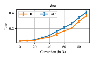
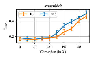
Figure 2: Classification. Testing risks (from Eq. 1) achieved by AC and IL on the “dna” and “svmguide2” datasets from LIBSVM as a function of corruption parameter $c$, when the corruption is as follows: for $y$ being the most present labels of the dataset, and $z^{\prime}\neq z$, $\operatorname{\mathbb{P}}\left(z^{\prime}\in S\,\middle|\,Y=z\right)=c\cdot\mathbf{1}_{z=y}$. Plotted intervals show the standard deviation on eight-fold cross-validation. Experiments were done with the Gaussian kernel. See all experimental details in Appendix B.

Real data experiment.

To compare IL and AC, we used LIBSVM datasets (Chang & Lin, 2011) on which we corrupted labels to simulate partial labelling. When the corruption is uniform, the two methods perform the same. Yet, when labels are unbalanced, such as in the “dna” and “svmguide2” datasets, and we only corrupt the most frequent label $y\in\mathcal{Y}$, the infimum loss performs better as shown in Fig. 2.

5.2 Ranking

Ranking consists in ordering $m$ items based on an input $x$ that is often the conjunction of a user $u$ and a query $q$, ($x=(u,q)$). An ordering can be thought as a permutation, that is, $\mathcal{Y}=\mathfrak{S}_{m}$. While designing a loss for ranking is intrinsincally linked to a voting system (Arrow, 1950), making it a fundamentally hard problem; Kemeny (1959) suggested to approach it through pairwise disagreement, which is current machine learning standard (Duchi et al., 2010), leading to the Kendall embedding

$$\varphi(y)=\left(\operatorname{sign}\left(y_{i}-y_{j}\right)\right)_{i<j\leq m},$$

and the Kendall loss (Kendall, 1938), with $C=m(m-1)/2$

$$\ell(y,z)=C-\varphi(y)^{T}\varphi(z).$$

Supervision often comes as partial order on items, e.g.,

$$S=\left\{y\in\mathfrak{S}_{m}\,\middle|\,y_{i}>y_{j}>y_{k},y_{l}>y_{m}\right\}.$$

It corresponds to fixing some coordinates in the Kendall embedding. In this setting, AC and SP are not consistent, as one can recreate a similar situation to the one in Sec. 4, considering $m=3$, $a=(1,2,3)$, $b=(2,1,3)$ and $c=(1,3,2)$ (permutations being represented with $(\sigma^{-1}(i))_{i\leq m}$), and supervision being most often $S=(1>3)=\left\{a,b,c\right\}$ and sometimes $S=(1>3>2)=\left\{c\right\}$.

Minimum feedback arc set.

Dealing with Kendall’s loss requires to solve problem of the form,

$$\operatorname*{arg\,min}_{y\in S}\left\langle c,\varphi(y)\right\rangle,$$

for $c\in\mathbb{R}^{m^{2}}$, and constraints due to partial ordering encoded in $S\subset\mathcal{Y}$. This problem is an instance of the constrained minimum feedback arc set problem.We provide a simple heuristic to solve it in Sec. B.5, which consists of approaching it as an integer linear program. Such heuristics are analyzed and refined for analysis purposes by Ailon et al. (2005); van Zuylen et al. (2007).

Algorithm specification.

At inference, the infimum loss requires to solve:

$$f_{n}(x)=\operatorname*{arg\,max}_{z\in\mathcal{Y}}\sup_{(y_{i})\in S_{i}}\sum_{i=1}^{n}\alpha_{i}(x)\left\langle\varphi(z),\varphi(y_{i})\right\rangle.$$ (7)

It can be approached with alternate minimization, initializing $\varphi(y_{i})\in\operatorname{Conv}(\varphi(S_{i}))$, by putting $0$ on unseen observed pairwise comparisons, then, iteratively, solving a minimum feedback arc set problem in $z$, then solving several minimum feedback arc set problems with the same objective, but different constraints in $(y_{i})$. This is done efficiently using warmstart on the dual simplex algorithm.

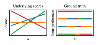
Figure 3: Ranking, experimental setting. Colors represent four different items to rank. Each item is associate to a utility function of $x$ shown on the left figure. From those scores, is retrieved an ordering $y$ of the items as represented on the right.

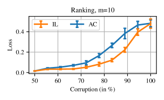
Figure 4: Ranking, results. Testing risks (from Eq. 1) achieved by AC and IL as a function of corruption parameter $c$. When $c=1$, both risks are similar at $0.5$. The simulation setting is the same as in Fig. 2. The error bars are defined as for Fig. 2, after cross-validation over eight folds. IL clearly outperforms AC.

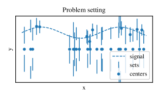
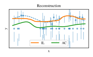
Figure 5: Partial regression on $\mathbb{R}$. In this setting we aim at recovering a signal $y(x)$ given upper and lower bounds on it amplitude, and in thirty percent of case, information on its phase, or equivalently in $\mathbb{R}$, its sign. IL clearly outperforms the baseline. Indeed AC is a particular ill-fitted method on such a problem, since it regresses on the barycenters of the resulting sets.

Synthetic experiments.

Let us consider $\mathcal{X}=[0,1]$ embodying some input features. Let $\{1,\dots,m\}$, $m\in\mathbb{N}$ be abstract items to order, each item being linked to a utility function $v_{i}\in\mathbb{R}^{\mathcal{X}}$, that characterizes the value of $i$ for $x$ as $v_{i}(x)$. Labels $y(x)\in\mathcal{Y}$ are retrieved by sorting $(v_{i}(x))_{i\leq m}$. To simulate a problem instance, we set $v_{i}$ as $v_{i}(x)=a_{i}\cdot x+b_{i}$, where $a_{i}$ and $b_{i}$ follow a standard normal distribution. Such a setting is illustrated in Fig. 3.

After sampling $x$ uniformly on $[0,1]$ and retrieving the ordering $y$ based on scores, we simulate partial labelling by randomly loosing pairwise comparisons. The comparisons are formally defined as coordinates of the Kendall’s embedding $(\varphi(y)_{jk})_{jk\leq m}$. To create non symmetric perturbations we corrupt more often items whose scores differ a lot. In other words, we suppose that the partial labelling focuses on pairs that are hard to discriminate. The corruption is set upon a parameter $c\in[0,1]$. In fact, for $m=10$, until $c=0.5$, our corruption is fruitless since it can most often be inverted based on transitivity constraint in ordering, while the problem becomes non-trivial with $c\geq 0.5$. In the latter setting, IL clearly outperforms AC on Fig. 4.

5.3 Partial regression

Partial regression is an example of non discrete partial labelling problem, where $\mathcal{Y}=\mathbb{R}^{m}$ and the usual loss is the Euclidean distance

$$\ell(y,z)=\left\|y-z\right\|^{2}.$$

This partial labelling problem consists of regression where observation are sets $S\subset\mathbb{R}^{m}$ that contains the true output $y$ instead that $y$. Among others, it arises for example in economical models, where bounds are preferred over approximation when acquiring training labels (Tobin, 1958). As an example, we will illustrate how partial regression could appear for some phase problems arising with physical measurements. Suppose a physicist want to measure the law between a vectorial quantity $Y$ and some input parameters $X$. Suppose that, while she can record the input parameters $x$, her sensors do not exactly measure $y$ but render an interval in which the amplitude $\left\|y\right\|$ lays and only occasionally render its phase $y/\left\|y\right\|$, in a fashion that leads to a set of candidates $S$ for $y$. The geometry over $\ell^{2}$ makes it a perfect example to showcase superiority of the infimum loss as illustrated in Fig. 5.

In this figure, we consider ${\cal Y}=\mathbb{R}$ and suppose that $Y$ is a deterministic function of $X$ as shown by the dotted blue line signal. If, for a given $x_{i}$, measurements only provides that $\left|y_{i}\right|\in[1,2]$ without the sign of $y_{i}$, a situation where the phase is lost, this correspond to the set $S_{i}=[-2,-1]\cup[1,2]$, explaining the shape of observed sets that are symmetric around the origin. Whenever the acquired data has no phase, which happen seventy percent of the time in our simulation, AC will target the set centers, explaining the green curve. On the other hand, IL is aiming at passing by each set, which explains the orange curve, crossing all blue bars.

6 Conclusions

In this paper, we deal with the problem of weakly supervised learning, beyond standard regression and classification, focusing on the more general case of arbitrary loss functions and structured prediction. We provide a principled framework to solve the problem of learning with partial labelling, from which a natural variational approach based on the infimum loss is derived. We prove that under some identifiability assumptions on the labelling process the framework is able to recover the solution of the original supervised learning problem. The resulting algorithm is easy to train and with strong theoretical guarantees. In particular we prove that it is consistent and we provide generalization error rates. Finally the algorithm is tested on simulated and real datasets, showing that when the acquisition process of the labels is more adversarial in nature, the proposed algorithm performs consistently better than baselines. This paper focuses on the problem of partial labelling, however the resulting mathematical framework is quite flexible in nature and it is interesting to explore the possibility to extend it to tackle also other weakly supervised problems, as imprecise labels from non-experts (Dawid & Skene, 1979), more general constraints over the set $(y_{i})_{i\leq n}$ (Quadrianto et al., 2009) or semi-supervision (Chapelle et al., 2006).

Appendix A Proofs

In the paper, we have implicitely considered $\mathcal{X},\mathcal{Y}$ separable and completely metrizable topological spaces, i.e. Polish spaces, allowing to consider probabilities. Moreover, we assumed that $\mathcal{Y}$ is compact, to have minimizer well defined. The observation space was considered to be the set of closed subsets of $\mathcal{Y}$ endowed with the Hausdorff distance, ${\cal S}={\operatorname{Cl}(\mathcal{Y}),d_{H}}$. As such, ${\cal S}$ is also a Polish metric space, inheriting this property from $\mathcal{Y}$ appBeer1993. In the following, we will show that the closeness of sets is important in order to switch from the minimum variability principle to the infimum loss.

In term of notations, we use the simplex notation $\Delta_{\cal A}$ to denote the space of Borel probability measures over the space ${\cal A}$. In particular, $\Delta_{\mathcal{X}\times\mathcal{Y}}$, $\Delta_{\mathcal{X}\times{\cal S}}$ and $\Delta_{\mathcal{X}\times\mathcal{Y}\times{\cal S}}$ are endowed with the weak-* topology and are Polish, inheriting the properties from original spaces appAliprantis2006. The fact that such spaces are Polish allows to define the conditional probabilities given $x\in\mathcal{X}$. We will denote this conditional probability $\rho|_{x}$ when, for example, $\rho\in\Delta_{\mathcal{X}\times\mathcal{Y}}$. Finally, we will denote by $\rho_{\mathcal{X}}$ the marginal of $\rho$ over $\mathcal{X}$.

Before diving into proofs, we would like to point out that many of our results are pointwise results. At an intuitive level, we only leverage the structure of the loss on the output space and aggregate those results over $\mathcal{X}$.

Remark (Going pointwise).

The learning frameworks in Eqs. 1, 2 and 4 are pointwise separable as their solutions can be written as aggregation of pointwise solutions appDevroye1996. More exactly, the partial labelling risk (and similarly the fully supervised one) can be expressed as

$${\cal R}_{S}(f)=\operatorname{\mathbb{E}}_{X}\left[{\cal R}_{S,X}(f(X))\right],$$

where the conditional risk reads,

$${\cal R}_{S,x}(z)=\operatorname{\mathbb{E}}_{S\sim\tau|_{x}}\left[L(z,S)\right],$$

with $\tau|_{x}$ the conditional distribution of $\left(S\,\middle|\,X=x\right)$. Thus, minimizing ${\cal R}_{S}$ globally for $f\in\mathcal{Y}^{\mathcal{X}}$ is equivalent to minimizing locally ${\cal R}_{S,x}$ for $f(x)$ for almost all $x$. Similarly, for Eq. 2,

$${\cal E}(\rho)=\inf_{f:\mathcal{X}\to\mathcal{Y}}\operatorname{\mathbb{E}}_{\rho}\left[\ell(f(X),Y)\right]=\operatorname{\mathbb{E}}_{X}\left[\inf_{z\in\mathcal{Y}}\operatorname{\mathbb{E}}_{Y\sim\rho|_{x}}\left[\ell(z,Y)\,\middle|\,X=x\right]\right].$$

Therefore studies on risk can be done pointwise on instances $(\ell,\rho|_{x},\tau|_{x})$, before integrating along $\mathcal{X}$. Actually, Props. 1, 1, 2 and 2 are pointwise results.

A.1 Proof of Prop. 1

Here we want to prove that when $\tau$ is non-ambigouous, then it is possible to define an optimal $\rho^{\star}$ that is deterministic on $\mathcal{Y}$, and that this $\rho^{\star}$ is characterized by solving Eq. 2.

Lemma 1.

When $\tau$ is non ambiguous, and there is one, and only one, deterministic distribution eligible for $\tau$. More exactly, if we write, for any $x\in\mathcal{X}$ in the support of $\tau_{\mathcal{X}}$, based on Def. 2, $S_{x}=\left\{y_{x}\right\}$, then this deterministic distribution is characterized as $\rho|_{x}=\delta_{y_{x}}$ almost everywhere.

Proof.

Let us consider a probability measure $\tau\in\Delta_{\mathcal{X}\times{\cal S}}$. We begin by working on the concept of eligibility. Consider $\rho\in\Delta_{\mathcal{X}\times\mathcal{Y}}$ eligible for $\tau$ and a suitable $\pi$ as defined in Def. 1. First of all, the condition that, for $y\in S$, $\operatorname{\mathbb{P}}_{\pi}\left(S\,\middle|\,Y=y\right)=0$, can be stated formally in term of measure as

$$\pi(\left\{(x,y,S)\in\mathcal{X}\times\mathcal{Y}\times{\cal S}\,\middle|\,y\notin S\right\})=0,$$

from which we deduced that, for $y\in\mathcal{Y}$ and $x\in\mathcal{X}$,

$$\rho|_{x}(y) =\pi|_{x}(\left\{y\right\}\times{\cal S})=\pi|_{x}(\left\{y\right\}\times\left\{S\in{\cal S}\,\middle|\,y\in S\right\})$$

$$\leq\pi|_{x}(\mathcal{Y}\times\left\{S\in{\cal S}\,\middle|\,y\in S\right\})=\tau|_{x}(\left\{S\in{\cal S}\,\middle|\,y\in S\right\}).$$

It follows that when $\rho$ is deterministic, if we write $\rho|_{x}=\delta_{y_{x}}$, then we have $\tau|_{x}(\left\{S\in{\cal S}\,\middle|\,y_{x}\in S\right\})=1,$ which means that $y_{x}$ is in all sets that are in the support of $\tau|_{x}$, or that, using notations of Def. 2, $y_{x}\in S_{x}$. So far, we have proved that if there exists a deterministic distribution, $\rho|_{x}=\delta_{y_{x}}$, that is eligible for $\tau|_{x}$, we have $y_{x}\in S_{x}$. Reciprocally, one can do the reverse derivations, to show that if $\rho|_{x}=\delta_{y_{x}}$, with $y_{x}\in S_{x}$, for all $x\in\mathcal{X}$, then $\rho$ is elgible for $\tau$ When $\tau$ is non-ambiguous, $S_{x}$ is a singleton and therefore, there could be only one deterministic eligible distribution for $\tau$, that is characterized in the lemma. ∎

Now we use the characterization of deterministic distribution through the minimization of the risk Eq. 1.

Lemma 2 (Deterministic characterization).

When $\mathcal{Y}$ is compact and $\ell$ proper, deterministic distribution are exactly characterized by minimum variability Eq. 2 as

$${\cal E}(\rho)=\inf_{f:\mathcal{X}\to\mathcal{Y}}\operatorname{\mathbb{E}}_{\rho}\left[\ell(f(X),Y)\right]=0.$$

Proof.

Let’s consider $\rho\in\Delta_{\mathcal{X}\times\mathcal{Y}}$, because $\mathcal{Y}$ is compact and $\ell$ continuous, we can consider $f_{\rho}$ a minimizer of ${\cal R}(f;\rho)$. Let’s now suppose that ${\cal R}(f_{\rho};\rho)=0$, since $\ell$ is non-negative, it means that almost everywhere

$$\operatorname{\mathbb{E}}_{Y\sim\rho|_{x}}\left[\ell(f_{\rho}(x),Y)\right]=0.$$

Suppose that $\rho|_{x}$ is not deterministic, then there is at least two points $y$ and $z$ in $\mathcal{Y}$ in its support, than, because $\ell$ is proper, we come to the absurd conclusion that

$$\operatorname{\mathbb{E}}_{Y\sim\rho|_{x}}\left[\ell(f_{\rho}(x),Y)\right]\geq\rho|_{x}(y)\ell(f_{\rho}(x),y)+\rho|_{x}(z)\ell(f_{\rho}(x),z)>0.$$

So ${\cal R}(f_{\rho};\rho)=0$ implies that $\rho$ is deterministic. Reciprocally, when $\rho$ is deterministic it is easy to show that the risk is minimized at zero. ∎

A.2 Proof of Thm. 1

At a comprehensive level, the Thm. 1 is composed of two parts:

• A double minimum switch, to take the minimum over $\rho$ before the minimum over $f$, and for which we need some compactness assumption to consider the joint minimum.

• A minimum-expectation switch, to take the minimum over $\rho\vdash\tau$ as a minimum $y\in S$ before the expectation to compute the risk, and for which we need some measure properties.

We begin with the minimum-expectation switch. To proceed with derivations, we need first to reformulate the concept of eligibility in Def. 1 in term of measures.

Lemma 3 (Measure eligibility).

Given a probability $\tau$ over $\mathcal{X}\times{\cal S}$, the space of probabilities over $\mathcal{X}\times\mathcal{Y}$ satisfying $\rho\vdash\tau$ is characterized by all probability measures of the form

$$\rho(C)=\int_{\mathcal{X}\times\mathcal{Y}\times{\cal S}}\mathbf{1}_{C}(x,y)\mathop{}\!\mathrm{d}\pi|_{x,S}(y)\mathop{}\!\mathrm{d}\tau(x,S),$$

for any $C$ a closed subset of $\mathcal{X}\times\mathcal{Y}$, and where $\pi$ is a probability measure over $\mathcal{X}\times\mathcal{Y}\times{\cal S}$ that satisfies $\pi_{\mathcal{X}\times{\cal S}}=\tau$ and $\pi|_{x,S}(S)=1$ for any $(x,S)$ in the support of $\tau$.

Proof.

For any $\rho$ that is eligible for $\tau$ there exists a suitable $\pi$ on $\mathcal{X}\times\mathcal{Y}\times{\cal S}$ as specified by Def. 1. Actually, the set of $\pi$ leading to an eligible $\rho:=\pi_{\mathcal{X}\times\mathcal{Y}}$ is characterized by satisfying $\pi_{\mathcal{X}\times{\cal S}}=\tau$ and

$$\pi(\{(x,y,S)\in\mathcal{X}\times\mathcal{Y}\times{\cal S}\leavevmode\nobreak\ |\leavevmode\nobreak\ y\notin S\})=0.$$

This last property can be reformulated with the complementary space as

$$\pi(\{(x,y,S)\in\mathcal{X}\times\mathcal{Y}\times{\cal S}\leavevmode\nobreak\ |\leavevmode\nobreak\ y\in S\})=1,$$

which equivalently reads, that for any $(x,S)$ in the support of $\tau$, we have

$$\pi|_{x,S}(S)=\pi|_{x,S}(\left\{y\in\mathcal{Y}\,\middle|\,y\in S\right\})=1.$$

Finally, using the conditional decomposition we have that, for $C$ a closed subset of $\mathcal{X}\times\mathcal{Y}$

$$\rho(C)=\pi_{\mathcal{X}\times\mathcal{Y}}(C)=\int_{\mathcal{X}\times\mathcal{Y}\times{\cal S}}\mathbf{1}_{C}(x,y)\mathop{}\!\mathrm{d}\pi(x,y,S)=\int_{\mathcal{X}\times\mathcal{Y}\times{\cal S}}\mathbf{1}_{C}(x,y)\mathop{}\!\mathrm{d}\pi|_{x,S}(y)\mathop{}\!\mathrm{d}\pi_{\mathcal{X}\times{\cal S}}(x,S),$$

which ends the proof since $\tau=\pi_{\mathcal{X}\times{\cal S}}$. ∎

We are now ready to state the minimum-expectation switch.

Lemma 4 (Minimum-Expectation switch).

For a probability measure $\tau\in\Delta_{\mathcal{X}\times{\cal S}}$, and measurable functions $\ell\in\mathbb{R}^{\mathcal{Y}\times\mathcal{Y}}$ and $f\in\mathcal{Y}^{\mathcal{X}}$, the infimum of eligible expectations of $\ell$ is the expectation of the infimum of $f$ over $S$ where $S$ is distributed according to $\tau$. Formally

$$\inf_{\rho\vdash\tau}\operatorname{\mathbb{E}}_{(X,Y)\sim\rho}\left[\ell(f(X),Y)\right]=\operatorname{\mathbb{E}}_{(X,S)\sim\tau}\left[\inf_{y\in S}\ell(f(X),y)\right].$$

Proof.

Before all, note that $(x,S)\to\inf_{y\in S}\ell(f(x),y)$ inherit measurability from $f$ allowing to consider such an expectation [see Theorem 18.19 of][and references therein for details]appAliprantis2006. Moreover, let us use Lem. 3 to reformulation the right handside problem as

$$\inf_{\rho\vdash\tau}\operatorname{\mathbb{E}}_{(X,Y)\sim\rho}\left[\ell(f(X),Y)\right]=\inf_{\pi\in{\cal M}}\int_{\mathcal{X}\times\mathcal{Y}\times{\cal S}}\ell(f(x),y)\mathop{}\!\mathrm{d}\pi_{x,S}(y)\mathop{}\!\mathrm{d}\tau(x,S).$$

Where we denote by ${\cal M}\subset\Delta_{\mathcal{X}\times\mathcal{Y}\times{\cal S}}$ the space of probability measures $\pi$ that satify the assumption of Lem. 3. We will now prove the equality by showing that both quantity bound the other one.

($\geq$).

To proceed with the first bound, notice that for $x\in\mathcal{X}$ and $S\in{\cal S}$, when $\pi|_{x,S}\in\Delta_{\mathcal{Y}}$ only charge $S$, i.e. if $\pi\in{\cal M}$, then

$$\int_{\mathcal{Y}}\ell(f(x),y)\mathop{}\!\mathrm{d}\pi_{x,S}(y)\geq\inf_{y\in S}\ell(f(x),y).$$

The first bound is then obtained by taking the expectation over $\tau$ of this poinwise property.

($\leq$).

For the second bound, we consider the function $Y\in\mathcal{Y}^{\mathcal{X}\times{\cal S}}$ define as

$$Y(x,S)=\operatorname*{arg\,min}_{y\in S}\ell(f(x),y).$$

Such a function is well defined since $S$ is compact due to the fact that $\mathcal{Y}$ is compact and ${\cal S}$ is the set of closed set. However, in more general cases, one can consider a sequence that minimize $\ell(f(x),y)$ rather than the argmin to show the same as what we are going to show. Now, if we define $\pi^{(f)}$ with $\pi^{(f)}_{\mathcal{X}\times{\cal S}}:=\tau$ and $\pi^{(f)}|_{x,S}:=\delta_{Y(x,S)}$, because $Y(x,S)$ is in $S$, we have that $\pi^{(f)}$ is in ${\cal M}$, so, for $x\in\mathcal{X}$ and $S\in{\cal S}$

$$\inf_{\pi\in{\cal M}}\int_{\mathcal{Y}}\ell(f(x),y)\mathop{}\!\mathrm{d}\pi_{x,S}(y)\leq\int_{\mathcal{Y}}\ell(f(x),y)\mathop{}\!\mathrm{d}\pi^{(f)}_{x,S}(y)=\ell(f(x),Y(x,S))=\inf_{y\in S}\ell(f(x),y).$$

We end the proof by integrating this over $\tau$. ∎ Now, we will move on to the minimum switch. First, we make sure that the infimum loss minimizer is well defined.

Lemma 5 (Infimum loss minimizer).

When $\mathcal{Y}$ is compact and the observed set are closed, there exists a measurable function $f_{S}\in\mathcal{Y}^{\mathcal{X}}$ that minimize the infimum loss risk

$${\cal R}_{S}(f_{S})=\inf_{f:\mathcal{X}\to\mathcal{Y}}{\cal R}_{S}(f),\qquad\text{where}\qquad{\cal R}_{S}(f)=\int\min_{y\in S}\ell(f(x),y)\mathop{}\!\mathrm{d}\tau(x,S).$$

The infimum on the right handside being a minimum because $S$ is a closed subset of $\mathcal{Y}$ compact, and therefore, is compact.

Proof.

First note that $d(y,y^{\prime})=\sup_{z\in\mathcal{Y}}\left|\ell(z,y)-\ell(z,y^{\prime})\right|$ is a metric on $\mathcal{Y}$ when $\ell$ is a proper loss. Indeed, triangular inequality holds trivially, moreover when $y=y^{\prime}$ then $d(y,y^{\prime})=0$, when $y\neq y^{\prime}$, by properness we have $\ell(y,y)=0$ and $d(y,y^{\prime})\geq\ell(y,y^{\prime})>0$. Moreover note that $L(z,S)=\min_{y\in S}\ell(z,y)$ is continuous and $1$-Lipschitz with respect to the topology induced by the Hausdorff distance $d_{H}$ based on $d$, indeed given two sets $S,S^{\prime}\in{\cal S}$

$$\left|L(z,S)-L(z,S^{\prime})\right| \leq\max\left\{\max_{y\in S}\min_{y^{\prime}\in S^{\prime}}\left|\ell(z,y)-\ell(z,y^{\prime})\right|,\leavevmode\nobreak\ \max_{y^{\prime}\in S^{\prime}}\min_{y\in S}\left|\ell(z,y)-\ell(z,y^{\prime})\right|\right\}$$

$$\leq\max\left\{\max_{y\in S}\min_{y^{\prime}\in S^{\prime}}d(y,y^{\prime}),\leavevmode\nobreak\ \max_{y^{\prime}\in S^{\prime}}\min_{y\in S}d(y,y^{\prime})\right\}=d_{H}(S,S^{\prime}).$$

The result of existence of a measurable $f_{S}$ minimizing ${\cal R}_{S}(f)=\int L(f(x),S)d\tau(x,S)$ follows by the compactness of $\mathcal{Y}$, the continuity of $L(z,S)$ in the first variable with respect to the topology induced by $d$, in the second with respect to the topology induced by $d_{H}$ and measurability of $\tau|_{x}$ in $x$, via Berge maximum theorem [see Thm. 18.19 of][and references therein]appAliprantis2006. ∎

We can state the minimum switch now.

Lemma 6 (Minimum switch).

When $\mathcal{Y}$ is compact, and observed sets are closed, solving the partial labelling through the minimum variability principle

$$f^{*}\in\operatorname*{arg\,min}_{f\in\mathcal{Y}^{\mathcal{X}}}\operatorname{\mathbb{E}}_{\rho^{\star}}\left[\ell(f(X),Y)\right],\qquad\text{with}\qquad\rho^{\star}\in\operatorname*{arg\,min}_{\rho\vdash\tau}\inf_{f\in\mathcal{Y}^{\mathcal{X}}}\operatorname{\mathbb{E}}_{\rho}\left[\ell(f(X),Y)\right].$$

can be done jointly in $f$ and $\rho$, and rewritten as

$$f^{*}\in\operatorname*{arg\,min}_{f\in\mathcal{Y}^{\mathcal{X}}}\inf_{\rho\vdash\tau}\operatorname{\mathbb{E}}_{\rho}\left[\ell(f(X),Y)\right].$$

Proof.

When $(\rho^{\star},f^{*})$ is a minimizer of the top problem, it also minimizes the joint problem $(\rho,f)\to{\cal R}(f;\rho)$, and we can switch the infimum order. The hard part is to show that when $f_{S}$ minimize the bottom risk, the infimum over $\rho$ is indeed a minimum. Indeed, we know from Lem. 4 that $f_{S}$ is characterized as a minimizer of the infimum risk ${\cal R}_{S}$, those are well defined as shown in precedent lemma. To $f_{S}$, we can associate $\rho_{S}:=\pi^{(f)}$ as defined in the proof of Lem. 4, which is due to the closeness of sets in ${\cal S}$ and the compactness of $\mathcal{Y}$. Indeed, $(f_{S},\rho_{S})$ minimize jointly the objective ${\cal R}(f,\rho)$, so we have that

$$\rho_{S}\in\operatorname*{arg\,min}_{\rho\vdash\tau}\inf_{f:\mathcal{X}\to\mathcal{Y}}{\cal R}(f;\rho),\qquad\text{and}\qquad f_{S}\in\operatorname*{arg\,min}_{f:\mathcal{X}\to\mathcal{Y}}{\cal R}(f;\rho_{S}).$$

From which we deduced that $\rho_{S}$ can be written as a $\rho^{\star}$ and $f_{S}$ as a $f^{*}$. ∎

Remark (A counter example when sets are not closed.).

The minimum switch relies on compactness assumption, that can be violated when the observed sets in ${\cal S}$ are not closed. Let us consider the case where $\mathcal{Y}=\mathbb{R}$, $\ell=\ell_{2}$ is the mean square loss. Consider the pointwise weak supervision

$$\tau=\frac{1}{2}\delta_{\mathbb{Q}}+\frac{1}{2}\delta_{\sqrt{2}\mathbb{Q}},$$

In this case, we have $\rho^{\star}=\delta_{0}$. Yet, for any $z$, we do have ${\cal R}_{S,x}(z)=0$ for any $z\in\mathbb{R}$. For example, if $z=\sqrt{2}$, one can consider

$$\rho_{n}=\frac{1}{2}\delta_{\sqrt{2}}+\frac{1}{2}\delta_{\frac{\left\lfloor 10^{n}\sqrt{2}\right\rfloor}{10^{n}}},$$

to show that $z\in\operatorname*{arg\,min}_{z\in\mathcal{Y}}\inf_{\rho\vdash\tau}{\cal R}(z,\rho)$. As one can see this is counter example is based on the fact that $\left\{\rho\,\middle|\,\rho\vdash\tau\right\}$ is not complete, so that there exists infimum of ${\cal R}_{x}(z,\rho)$ that are not minimum such as ${\cal R}_{x}(\sqrt{2},\delta_{\sqrt{2}})$.

A.3 Proof of Thm. 2

If $\tau$ is not ambiguous, then, almost surely for $x\in\mathcal{X}$, if $y_{x}$ is the only element in $S_{x}$ of Def. 2, we know that $\rho^{\star}|_{x}=\delta_{y_{x}}$, and consequently we derive $f^{*}(x)=y_{x}$, so for it to be consistent with $f_{0}$, we need that $f_{0}(x)=y_{x}$.

Moreover, because $\tau$ is a weaking of $\rho_{0}$, $\rho_{0}$ is eligible for $\tau$. When $\rho_{0}$ is deterministic, we know from considerations in the proof of Lem. 1, that it is $\rho^{\star}$, the only deterministic distribution eligible for $\tau$. Thus, in fact, the condition $S_{x}=\left\{f_{0}(x)\right\}$ is implied by $\rho_{0}$ deterministic.

A.4 Proof of Prop. 2

When $\tau$ is not ambiguous, we know from Prop. 1, that $\rho^{\star}$ is deterministic. Let us write $\rho^{\star}|_{x}=\delta_{y_{x}}$, we have $f^{*}(x)=y_{x}$, and ${\cal R}_{x}(f^{*})=0$, moreover, because $y_{x}$ is in every $S$ in the support of $\tau|_{S}$, then ${\cal R}_{S,x}(f^{*})=0$. Similarly to the bound given by appCour2011 for the 0-1 loss, we have

$${\cal R}_{S,x}(z) =\operatorname{\mathbb{E}}_{S\sim\tau|_{x}}[\inf_{z^{\prime}\in S}\ell(z,z^{\prime})]=\sum_{S;z\notin S}\inf_{z^{\prime}\notin S}\ell(z,z^{\prime})\operatorname{\mathbb{P}}_{S\sim\tau|_{x}}(S)$$

$$\geq\inf_{z^{\prime}\neq z}\ell(z,z^{\prime})\operatorname{\mathbb{P}}_{S\sim\tau|_{x}}(z\notin S)\geq\inf_{z^{\prime}\neq z}\ell(z,z^{\prime})\eta,$$

while ${\cal R}_{x}(z)=\ell(z,y)$, so we deduce locally

$${\cal R}_{x}(z;\rho^{\star}|_{x})-{\cal R}_{x}(f^{*}(x);\rho^{\star}|_{x}) \leq\frac{\ell(z,y)}{\inf_{z^{\prime}\neq z}\ell(z,z^{\prime})}\eta^{-1}\left({\cal R}_{S,x}(z)-{\cal R}_{S,x}(f^{*}(x))\right)$$

$$\leq e^{\nu}\eta^{-1}\left({\cal R}_{S,x}(z)-{\cal R}_{S,x}(f^{*}(x))\right).$$

Integrating over $x$ this last equation gives us the bound in Prop. 2.

A.5 Refined bound analysis of Prop. 2

The constant $C$ that appears in Prop. 2 is the result of controlling separately the corruption process and the discrepancy of the loss. Indeed, they can be controlled together, leading to a better constant. To relates the two risk ${\cal R}$ and ${\cal R}_{S}$, we will consider the pointwise setting $\tau\in\Delta_{2^{\mathcal{Y}}}$ and $\rho_{0}\in\Delta_{\mathcal{Y}}$ that satisfies $\rho_{0}\vdash\tau$, we will also consider a prediction $z\in\mathcal{Y}$.

Proposition 3 (Bound refinement).

When $\mathcal{Y}$ is discrete and $\tau$ not ambiguous, the best $C$ that verifies Eq. 6 in the pointwise setting $\tau\in\Delta_{2^{\mathcal{Y}}}$ is maximum of $\lambda^{-1}$, for $\lambda\in[0,1]$ such that there exists a point $z\neq y$ and signed measured $\sigma$ that verify ${\cal R}(z;\sigma)=0$ and such that $\sigma+\lambda\delta_{y}+(1-\lambda)\delta_{z}$ is a probabily measure that is eligible for $\tau$.

Proof.

First, let’s extend our study to the space ${\cal M}_{\mathcal{Y}}$ of signed measure over $\mathcal{Y}$. We extend the risk definition in Eq. 1 to any signed measure $\mu\in{\cal M}_{\mathcal{Y}}$, with

$${\cal R}_{x}(z;\mu)=\int_{\mathcal{Y}}\ell(z,y)\mathop{}\!\mathrm{d}\mu(y).$$

Note that the risk is a linear function of the distribution $\mu$. Two spaces are going to be of particular interest, the one of measure of mass one ${\cal M}_{\mathcal{Y},1}$, and the one of measure of mass null ${\cal M}_{\mathcal{Y},0}$, where

$${\cal M}_{\mathcal{Y},p}=\left\{\mu\in{\cal M}\,\middle|\,\mu(\mathcal{Y})=p\right\}.$$

Let’s now relates for a $\rho_{0}$, $\tau$ and $z$, the risk ${\cal R}_{x}(z;\rho_{0})$ and ${\cal R}_{S,x}(z)$. To do so, we introduce the space of signed measures of null mass, that could be said orthonal to $(\ell(z,y))_{y\in\mathcal{Y}}$, formally

$$D_{z}=\left\{\mu\in{\cal M}_{\mathcal{Y},0}\,\middle|\,{\cal R}_{x}(z;\mu)=0\right\}.$$

There is two alternatives: (1) either ${\cal R}_{x}(z;\rho_{0})=0$, and so ${\cal R}_{S,x}(z)=0$ too, and we have relates the two risk; (2) either ${\cal R}_{x}(z,\rho_{0})\neq 0$, and the space ${\cal M}_{\mathcal{Y},1}$ can be decomposed as

$${\cal M}_{\mathcal{Y},1}=D_{z}+\left\{\lambda\rho_{0}+(1-\lambda)\delta_{z}\,\middle|\,\lambda\in\mathbb{R}\right\}.$$

To prove it take $\mu\in{\cal M}_{\mathcal{Y},1}$, and use linearity of the risk after writing

$$\mu=\lambda\rho_{0}+(1-\lambda)\delta_{z}+\left(\mu-(\lambda\rho_{0}+(1-\lambda)\delta_{z})\right),\qquad\text{with}\qquad\lambda=\frac{{\cal R}_{x}(z,\mu)}{{\cal R}_{x}(z,\rho_{0})}.$$

For such a $\mu$, using the linearity of the risk, and the properness of the loss, if we denote by $d_{z}$ the part in $D_{z}$ of the last decomposition, we have

$${\cal R}_{x}(z;\mu)=\lambda{\cal R}_{x}(z;\rho_{0})+(1-\lambda){\cal R}_{x}(z;\delta_{z})+{\cal R}_{x}(z;d_{z})=\lambda{\cal R}_{x}(z;\rho_{0})$$

If we denote by $R_{\tau}=\left\{\rho\in\Delta_{\mathcal{Y}}\,\middle|\,\rho\vdash\tau\right\}$, we can conclude that

$$\frac{{\cal R}_{S,x}(z)}{{\cal R}_{x}(z;\rho_{0})}=\inf\left\{\lambda\,\middle|\,(\lambda\rho_{0}+(1-\lambda)\delta_{z})\in R_{\tau}+D_{z}\right\}.$$

Finally, when $\tau$ is not ambiguous, we know that $\rho^{\star}$ is deterministic, and if $\rho_{0}$ is deterministic then $\rho_{0}=\rho^{\star}$. In this case, there exists a $y$ such that $\rho_{0}=\delta_{y}$, and we can suppose this $y$ different of $z$ otherwise ${\cal R}_{x}(z;\rho_{0})=0$. In this case, we also have ${\cal R}_{x}(z^{*})={\cal R}_{S,x}(z^{*})=0$ with $z^{*}=y$, and thus the excess of risk to relates in Eq. 6 is indeed the relation between the two risks.

Figure 6: Geometrical understanding of Prop. 3, showing the link between the infimum and the fully supervised risk. The drawing is set in the affine span of the simplex ${\cal M}_{\mathcal{Y},1}$, where we identify $a$ with $\delta_{a}$. The underlying instance $(\ell,\tau)$ is taken from Sec. 4, and can be linked to the setting of Prop. 3 with $z=b$, $y=c$. Are represented in the simplex the level curves of the function $\rho\rightarrow{\cal R}(z;\rho)$. Based on this drawing, one can recover ${\cal R}_{S}(b)={\cal R}(b)/4$, which is better than the bound given in Prop. 2.

∎

Remark (Prop. 3 as a variant of Thales theorem).

Prop. 3 can be seen as a variant of the Thales theorem. Indeed, with the geometrical embedding $\pi$ of the simplex in $\mathbb{R}^{\mathcal{Y}}$, $\pi(\rho)=(\rho(y))_{y\in\mathcal{Y}}$, one can have, with $d$ the Euclidean distance

$$\frac{{\cal R}_{S,x}(z)}{{\cal R}_{x}(z;\rho_{0})}=\frac{d(\pi(\delta_{z}+D_{z}),\pi(R_{\tau}))}{d(\pi(\delta_{z}+D_{z}),\pi(\rho_{0}))}.$$

And conclude by using the following variant of Thales theorem, that can be derived from Fig. 7: For $x,y,z\in\mathbb{R}^{d}$, and $S\subset\mathbb{R}^{d}$, with $d$ the Euclidean distance, if $y\in S$, $d(z+x^{\perp},S)=\gamma d(z+x^{\perp},y)$, where

$$\gamma=\min\left\{\left|\lambda\right|\,\middle|\,\lambda\in\mathbb{R},(\lambda y+(1-\lambda)z+x^{\perp})\cap S\neq\emptyset\right\}.$$

More over, notice that if $S$ is contains in the half space that contains $y$ regarding the cut with the hyperplane $z+x^{\perp}$, $\lambda$ can be restricted to be in $[0,1]$.

Figure 7: A variant of Thales theorem.

Remark (Active labelling).

When annotating data, as a partial labeller, you could ask yourself how to optimize your labelling. For example, suppose that you want to poll a population to retrieved preferences among a set of presidential candidates. Suppose that for a given polled person, you can only ask her to compare between four candidates. Which candidates would you ask her to compare? According to the questions you are asking, you will end up with different sets of potential weak distribution $\tau$. If aware of the problem $\ell$ that your dataset is intended to tackle, and aware of a constant $C=C(\ell,\tau)$ that verify Eq. 6, you might want to design your questions in order to maximize on average over potential $\tau$, the quantity $C(\ell,\tau)$. An example where $\tau$ is not well designed according to $\ell$ is given in Fig. 8.

Figure 8: Example of a bad link between $\tau$ and $\ell$. Same representation as Fig. 6 with a different instance where $\tau=\frac{1}{2}\delta_{\left\{a,c\right\}}+\frac{1}{2}\delta_{\left\{b,c\right\}}$ and $\ell(b,a)=0$, $\ell(b,c)=1$. In this example $C_{\ell}(\tau)=+\infty$, and the infimum loss is $0$ on $\mathcal{Y}$ and therefore not consistent. Given the loss structure, partial labelling acquisition should focus on specifying sets that does not intersect $\left\{a,b\right\}$. Note that this instance violate the proper loss assumption, explaining its inconsistency.

A.6 Proof of Thms. 3 and 4

Firt note that, since ${\cal R}_{S}(f)$ is characterized by ${\cal R}_{S}(f)=\mathbb{E}_{(x,S)\sim\tau}\min_{u\in S}\ell(f(x),u)$, then the problem

$$f^{*}=\operatorname*{arg\,min}_{f:\mathcal{X}\to\mathcal{Y}}{\cal R}_{S}(f)=\operatorname*{arg\,min}_{f:\mathcal{X}\to\mathcal{Y}}\operatorname{\mathbb{E}}_{(x,S)\sim\tau}\left[\min_{y\in S}\ell(f(x),y)\right].$$

can be considered as an instance of structured prediction with loss $L(z,S)=\min_{y\in S}\ell(f(x),y)$. The framework for structured prediction presented in appCiliberto2016, and extended in appCiliberto2020, provides consistency and learning rates in terms of the excess risk ${\cal R}_{S}(f_{n})-{\cal R}_{S}(f^{*})$ when $f^{*}$ is estimated via $f_{n}$ defined as in Eq. 7 and when the structured loss $L$ admits the decomposition

$$L(z,S)=\langle\psi(z),\varphi(S)\rangle_{\cal H},$$

for a separable Hilbert space ${\cal H}$ and two maps $\psi:\mathcal{Y}\to{\cal H}$ and $\varphi:{\cal S}\to{\cal H}$. Note that since $\mathcal{Y}$ is finite $L$ always admits the decomposition, indeed the cardinality of $\mathcal{Y}$ is finite, i.e., $|\mathcal{Y}|<\infty$ and $|{\cal S}|=2^{|\mathcal{Y}|}$. Choose an ordering for the elements in $\mathcal{Y}$ and in ${\cal S}$ and denote them respectively $o_{\mathcal{Y}}:\mathbb{N}\to\mathcal{Y}$ and $o_{\cal S}:\mathbb{N}\to{\cal S}$. Let $n_{\mathcal{Y}}:\mathcal{Y}\to\mathbb{N}$ the inverse of $o_{\mathcal{Y}}$, i.e. $o_{\mathcal{Y}}(n_{\mathcal{Y}}(y))=y$ and $n_{\mathcal{Y}}(o_{\mathcal{Y}}(i))=i$ for $y\in\mathcal{Y}$ and $i\in{1,\dots,|\mathcal{Y}|}$, define analogously $n_{\cal S}$. Now let ${\cal H}=\mathbb{R}^{|\mathcal{Y}|}$ and define the matrix $B\in\mathbb{R}^{|\mathcal{Y}|\times 2^{|\mathcal{Y}|}}$ with element $B_{i,j}=L(o_{\mathcal{Y}}(i),o_{\cal S}(j))$ for $i=1,\dots,|\mathcal{Y}|$ and $j=1,\dots,2^{|\mathcal{Y}|}$, then define

$$\psi(z)=e^{|\mathcal{Y}|}_{n_{\mathcal{Y}}(z)},\quad\varphi(S)=Be^{2^{|\mathcal{Y}|}}_{n_{\cal S}(S)},$$

where $e^{k}_{i}$ is the $i$-th element of the canonical basis of $\mathbb{R}^{k}$. We have that

$$\langle\psi(z),\varphi(S)\rangle_{\cal H}=\langle e^{|\mathcal{Y}|}_{n_{\mathcal{Y}}(z)},Be^{2^{|\mathcal{Y}|}}_{n_{\cal S}(S)}\rangle_{R^{|\mathcal{Y}|}}=B_{n_{\mathcal{Y}}(z),n_{\cal S}(S)}=L(i_{\mathcal{Y}}(n_{\mathcal{Y}}(z)),i_{\cal S}(n_{\cal S}(S)))=L(z,S),$$

for any $z\in\mathcal{Y},S\in{\cal S}$. So we can apply Theorem 4 and 5 of appCiliberto2016 [see also their extended forms in Theorem 4 and 5 of][]appCiliberto2020. The last step is to connect the excess risk on ${\cal R}_{S}$ with the excess risk on ${\cal R}(f,\rho^{\star})$, which is done by our comparison inequality in Prop. 2.

Remark (Illustrating the consistency in a discrete setting).

Suppose that $\tau_{|x}$ has been approximate, as a signed measure $\hat{\tau}_{|x}=\sum_{i=1}^{n}\alpha_{i}(x)\delta_{S_{i}}$. After renormalization, one can represent it with as a region $R_{\hat{\tau}_{|x}}$ in the affine span of $\Delta_{\mathcal{Y}}$. Retaking the settings of Sec. 4, suppose that

$$\hat{\tau}(\left\{a,b\right\})=\frac{1}{2},\qquad\hat{\tau}(\left\{c\right\})=\frac{1}{2},\qquad\hat{\tau}(\left\{a,c\right\})=\frac{1}{4},\qquad\hat{\tau}(\left\{a,b,c\right\})=-\frac{1}{4}.$$

This corresponds to the region $R_{\hat{\tau}}$ represented in Fig. 9. It leads to a disambiguation $\hat{\rho}$ that minimizes ${\cal E}$, Eq. 2, inside this space as

$$\hat{\rho}(a)=\frac{1}{2},\qquad\hat{\rho}(b)=-\frac{1}{4},\qquad\hat{\rho}(c)=\frac{3}{4},$$

and to the right prediction $\hat{z}=c$, since $\hat{\rho}$ felt in the decision region $R_{c}$. As the number of data augments, $\mathbb{R}_{\hat{\rho}}$ converges towards $R_{\tau}$, so does $\hat{\rho}$ toward $\rho^{\star}$ and the risk ${\cal R}(\hat{f})$ towards its minimum.

Figure 9: Understanding convergence of the algorithm in Eq. 7. Our method is approximating $\tau$ as a signed measured $\hat{\tau}$, which leads to $R_{\hat{\tau}}$ in dark gray compared to the ground truth $R_{\tau}$ in light gray. The disambiguation of $\hat{\rho}$ and $\rho^{\star}$ is done on those two domains with the same objective ${\cal E}$, Eq. 2, which level curves are represented with light lines.

A.7 Understanding of the average and the supremum loss

For the average loss, if there is discrepancy in the loss $\nu>0$, then there exists $a,b,c$ such that $\ell(b,c)=(1+\varepsilon)\ell(a,b)$, for some $\varepsilon>0$. In this case, one can recreate the example of Sec. 4 by considering $\rho_{0}=\rho^{\star}=\delta_{c}$ and

$$\tau=\lambda\delta_{\left\{c\right\}}+(1-\lambda)\delta_{\left\{a,b,c\right\}},\qquad\text{with}\qquad\lambda=\frac{1}{2}\frac{\varepsilon}{3\ell(a,b)+\varepsilon},$$

to show the inconsistency of the average loss. Similarly supposing, without loss of generality that $\ell(a,c)\in\left[\ell(a,b),\ell(b,c)\right]$, the case where $\rho_{0}=\rho^{\star}=\delta_{b}$ and

$$\tau=\lambda\delta_{\left\{b\right\}}+(1-\lambda)\delta_{\left\{a,b,c\right\}},\qquad\text{with}\qquad\lambda=\frac{1}{2}\min\left(\frac{\varepsilon}{1+\varepsilon},\frac{1+\varepsilon-x}{2+\varepsilon-x}\right),\qquad x=\frac{\ell(a,c)}{\ell(a,b)},$$

will fail the supremum loss, which will recover $z^{*}=a$, instead of $z^{*}=b$.

Appendix B Experiments

B.1 Classification

Let consider the classification setting of Sec. 5.1. The infimum loss reads $L(z,S)=\mathbf{1}_{z\notin S}$. Given a weak distribution $\tau$, the infimum loss is therefore solving for

$$f(x)\in\operatorname*{arg\,min}_{z\in\mathcal{Y}}\operatorname{\mathbb{E}}_{S\sim\tau|_{x}}\left[L(z,S)\right]=\operatorname*{arg\,min}_{z\in\mathcal{Y}}\operatorname{\mathbb{E}}_{S\sim\tau|_{x}}\left[\mathbf{1}_{z\notin S}\right]=\operatorname*{arg\,min}_{z\in\mathcal{Y}}\operatorname{\mathbb{P}}_{S\sim\tau|_{x}}(z\notin S)=\operatorname*{arg\,max}_{z\in\mathcal{Y}}\operatorname{\mathbb{P}}_{S\sim\tau|_{x}}(z\in S).$$

Given data, $(z_{i},S_{i})$ our estimator consists in approximating the conditional distributions $\tau|_{x}$ as

$$\hat{\tau}|_{x}=\sum_{i=1}^{n}\alpha_{i}(x)\delta_{S_{i}},$$

from which we deduce the inference formula, that we could also derived from Eq. 7,

$$\hat{f}(x)\in\operatorname*{arg\,max}_{z\in\mathcal{Y}}\sum_{i=1}^{n}\alpha_{i}(x)\mathbf{1}_{z\in S_{i}}=\operatorname*{arg\,max}_{z\in\mathcal{Y}}\sum_{i;z\in S_{i}}\alpha_{i}(x).$$

B.1.1 Complexity Analysis

The complexity of our algorithm Eq. 7 can be split in two parts:

• a training part, where given $(x_{i},S_{i})$ we precompute quantities that will be useful at inference.

• an inference part, where given a new $x$, we compute the corresponding prediction $\hat{f}(x)$.

In the following, we will review the time and space complexity of both parts. We give this complexity in term of $n$ the number of data and $m$ the number of items in $\mathcal{Y}$. Results are summed up in Tab. 1.

Table 1: Complexity of our algorithm for classification.

Complexity	Time	Space
Training	${\cal O}(n^{2}(n+m))$	${\cal O}(n(n+m))$
Inference	${\cal O}(nm)$	${\cal O}(n+m)$

Training.

Let us suppose that computing $L(y,S)=\mathbf{1}_{y\notin S}$ can be done in a constant cost that does not depend on $m$. We first compute the following matrices in ${\cal O}(nm)$ and ${\cal O}(n^{2})$ in time and space.

$$L=(L(y,S_{i}))_{i\leq n,y\in\mathcal{Y}}\in\mathbb{R}^{n\times m},\qquad K_{\lambda}=(k(x_{i},x_{j})+n\lambda\delta_{i=j})_{ij}\in\mathbb{R}^{n\times n}.$$

We then solve the following, based on the _gesv routine of Lapack, in ${\cal O}(n^{3}+n^{2}m)$ in time and ${\cal O}(n(n+m))$ in space [see][for details]appGolub1996

$$\beta=K_{\lambda}^{-1}L\in\mathbb{R}^{n\times m}.$$

Inference.

At inference, we first compute in ${\cal O}(n)$ in both time and space

$$v(x)=(k(x,x_{i}))_{i\leq n}\in\mathbb{R}^{n}.$$

Then we do the following multiplication in ${\cal O}(nm)$ in time and ${\cal O}(m)$ in space,

$${\cal R}_{S,x}=v(x)^{T}\beta\in\mathbb{R}^{m}.$$

Finally we take the minimum of ${\cal R}_{S,x}(z)$ over $z$ in ${\cal O}(m)$ in time and ${\cal O}(1)$ in space.

B.1.2 Baselines

The average loss is really similar to the infimum loss, it reads

$$L_{\textit{ac}}(z,S)=\frac{1}{\left|S\right|}\sum_{y\in S}\ell(z,y)=1-\frac{\mathbf{1}_{z\in S}}{\left|S\right|}\simeq\frac{1}{\left|S\right|}\cdot\mathbf{1}_{z\notin S}=\frac{1}{\left|S\right|}L(z,S).$$

Following similar derivations to the one for the infimum loss, given a distribution $\tau$, one can show that the average loss is solving for

$$f_{\textit{ac}}(x)\in\operatorname*{arg\,max}_{z\in\mathcal{Y}}\sum_{S;z\in S}\frac{1}{\left|S\right|}\tau|_{x}(S),$$

which is consistent when $\tau$ is not ambiguous. The difference with the infimum loss is due to the term in $\left|S\right|$. It can be understood as an evidence weight, giving less importance to big sets that do not allow to discriminate efficiently between candidates. Given data $(x_{i},S_{i})$, it leads to the estimator

$$\hat{f}_{\textit{ac}}(x)\in\operatorname*{arg\,min}_{z\in\mathcal{Y}}\sum_{i;z\in S_{i}}\frac{\alpha_{i}(x)}{\left|S_{i}\right|}.$$

The supremum loss is really conservative since

$$L_{\textit{sp}}(z,S)=\sup_{y\in S}\ell(y,z)=\sup_{y\in S}\mathbf{1}_{y\neq z}=\mathbf{1}_{S\neq\left\{z\right\}}.$$

It is solving for

$$f(x)\in\operatorname*{arg\,max}_{z\in\mathcal{Y}}\tau|_{x}(\left\{z\right\}),$$

which empirically correspond to discarding all the set with more than one element

$$\hat{f}_{\textit{sp}}(x)\in\operatorname*{arg\,min}_{z\in\mathcal{Y}}\sum_{i;S_{i}=\left\{z\right\}}\alpha_{i}(x).$$

Note that $\tau$ could be not ambiguous while charging no singleton, in this case, the supremum loss is not informative, as its risk is the same for any prediction.

B.1.3 Corruptions on the LIBSVM datasets

To illustrate the dynamic of our method versus the average baseline, we used LIBSVM datasets appChang2011, that we corrupted by artificially adding false class candidates to transform fully supervised pairs $(x,y)$ into weakly supervised ones $(x,S)$. We experiment with two types of corruption process.

• A uniform one, reading, with the $\mu$ of Def. 1, for $z\neq y$,

  $$\operatorname{\mathbb{P}}_{(Y,S)\sim\mu|_{\mathcal{Y}\times 2^{\mathcal{Y}}}}\left(z\in S\,\middle|\,Y=y\right)=c.$$

  with $c$ a corruption parameter that we vary between zero and one. In this case, the average loss and the infimum one works the same as shown on Fig. 10.

• A skewed one, where we only corrupt pair $(x,y)$ when $y$ is the most present class in the dataset. More exactly, if $y$ is the most present class in the dataset, for $z\in\mathcal{Y}$, and $z^{\prime}\neq z$, our corruption process reads

  $$\operatorname{\mathbb{P}}_{(Y,S)\sim\mu|_{\mathcal{Y}\times 2^{\mathcal{Y}}}}\left(z^{\prime}\in S\,\middle|\,Y=z\right)=c\cdot\mathbf{1}_{z=y}.$$

  In unbalanced dataset, such as the “dna” and “svmguide2” datasets, where the most present class represent more than fifty percent of the labels as shown Tab. 2, this allows to fool the average loss as shown Fig. 2. Indeed, this corruption was designed to fool the average loss since we knew of the evidence weight $\frac{1}{\left|S\right|}$ appearing in its solution.

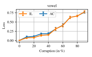
Figure 10: Classification. Testing risks (from Eq. 1) achieved by AC and IL on the “segment” and “vowel” datasets from LIBSVM as a function of corruption parameter $c$, when the corruption is uniform, as described in Sec. B.1.3.

Table 2: LIBSVM datasets characteristics, showing the number of data, of classes, of input features, and the proportion of the most present class when labels are unbalanced.

Dataset	Data ($n$)	Classes ($m$)	Features ($d$)	Balanced	Most present
Dna	2000	3	180	$\times$	52.6%
Svmguide2	391	3	20	$\times$	56.5%
Segment	2310	7	19	$\checkmark$	-
Vowel	528	11	10	$\checkmark$	-

B.1.4 Reproducibility specifications

All experiments were run with Python, based on NumPy library. Randomness was controlled by instanciating the random seed of NumPy to $0$ before doing any computations. Results of Figs. 2 and 10 were computed by using eight folds, and trying out several hyperparameters, before keeping the set of hyperparameters that hold the lowest mean error over the eight folds. Because we used a Gaussian kernel, there was two hyperparameters, the Gaussian kernel parameter $\sigma$, and the regularization parameter $\lambda$. We search for the best hyperparameters based on the heuristic

$$\sigma=c_{\sigma}d,\qquad\lambda=c_{\lambda}n^{-1/2},$$

where $d$ is the dimension of the input $\mathcal{X}$ (or the number of features), and where the Gaussian kernel reads

$$k(x,x^{\prime})=\exp\left(-\frac{\left\|x-x^{\prime}\right\|^{2}}{2\sigma^{2}}\right).$$

We tried $c_{\sigma}\in\left\{10,5,1,.5,.1,.01\right\}$ and $c_{\lambda}\in\left\{10^{i}\,\middle|\,i\in\left\llbracket 3,-3\right\rrbracket\right\}$.

B.2 Ranking

Consider the ranking setting of Sec. 5.2, where $\mathcal{Y}=\mathfrak{S}_{m}$, $\varphi$ is the Kendall’s embedding and the loss is equivalent to $\ell(z,y)=-\varphi(y)^{T}\varphi(z)$.

B.2.1 Complexity Analysis

Given data $(x_{i},S_{i})$, our algorithm is solving at inference for

$$f(x)\in\operatorname*{arg\,min}_{z\in\mathcal{Y}}\inf_{y_{i}\in S_{i}}-\sum_{i=1}^{n}\alpha_{i}(x)\varphi(z)^{T}\varphi(y_{i})=\operatorname*{arg\,max}_{z\in\mathcal{Y}}\sup_{y_{i}\in S_{i}}\sum_{i=1}^{n}\alpha_{i}(x)\varphi(z)^{T}\varphi(y_{i})$$

We solved it through alternate minimization, by iteratively solving in $z$ for

$$\varphi(z)^{(t+1)}=\operatorname*{arg\,max}_{\xi\in\varphi(\mathcal{Y})}\left\langle\xi,\sum_{i=1}^{n}\alpha_{i}(x)\varphi(y_{i})^{(t)}\right\rangle,$$

and solving for each $y_{i}$ for

$$\varphi(y_{i})^{(t+1)}=\operatorname*{arg\,max}_{\xi\in\varphi(S_{i})}\alpha_{i}(x)\left\langle\xi,\varphi(z)\right\rangle.$$

We initialize the problem with the coordinates of $\varphi(y_{i})$ put to 0 when not specified by the constraint $y_{i}\in S_{i}$. Those two problems are minimum feedback arc set problems, that are NP-hard in $m$, meaning that one has to check for all potential solutions, and there is $m!$ of them, which is the cardinal of $\mathfrak{S}_{m}$. We suggest to solve them using an integer linear programming (ILP) formulation that we relax into linear programming as explained in Sec. B.5. All the problem in $y_{i}$ share the same objective, up to a change in sign, but different constraint $\xi\in\varphi(S_{i})$, such a setting is particularily suited for warmstart on the dual simplex algorithm to solve efficiently one after the other the linear programs associated to each $y_{i}$.

To give numbers, at training time, we compute the inverse $K_{\lambda}^{-1}$ in ${\cal O}(n^{3})$ in time and ${\cal O}(n^{2})$ in space, and at inference we compute $\alpha(x)K_{\lambda}^{-1}v(x)$ in ${\cal O}(n^{2})$ in time and ${\cal O}(n)$ in space, before solving iteratively $n$ NP-hard problem in $m$ of complexity $n\textit{NP}(m)$, that cost $nm^{2}$ in space to represent using Cplex Cplex, if we allows our self $e$ iterations, the inference complexity is ${\cal O}(n^{2}+e\,n\,\textit{NP}(m))$ in time and ${\cal O}(nm^{2})$ in space.

B.2.2 Baselines

The supremum loss is really similar to the infimum loss, only changing an infimum by a supremum. However, algorithmically, this change leads to solving for a local sadle point rather than solving for a local minimum. While the latter are always defined, there might be instances where no sadle point exists. In this case, the supremum optimization might stall without getting to any stable solution, and the user might consider stopping the optimization after a certain number of iteration and outputting the current state as a solution.

The average loss, despite its simple formulation does not lead to an easy implementation either. Indeed, when given a set $S$, the average loss is implicitely computing the center of this set $c(S)$, and replacing $L_{\textit{ac}}(z,S)$ by $\ell(z,c(S))$, more exactly

$$L_{\textit{ac}}(z,S)\simeq-\frac{1}{\left|S\right|}\sum_{y\in S}\varphi(z)^{T}\varphi(y)=-\varphi(y)^{T}\left(\frac{1}{\left|S\right|}\sum_{y\in S}\varphi(y)\right).$$

To compute the center $\left(\frac{1}{\left|S\right|}\sum_{y\in S}\varphi(y)\right)$, we sample $c_{k}\sim{\cal N}(0,I_{m^{2}})$, solve the resulting minimum feedback arc set problem, with the constraint $y\in S$, and end up with solutions $\varphi(y_{k})$. After removing duplicates, we estimate the average with the empirical one. Note that this work is done at training, leading the average loss to have a quite good inference complexity in ${\cal O}(nm+\textit{NP}(m))$ in time.

B.2.3 Synthetic example: ordering lines

In the following, we explain our synthetic example of Sec. 5.2. It correspond of choosing $\mathcal{X}=[0,1]$, choose $m$ a number of items, simulate $a,b\sim{\cal N}(0,I_{m})$, compute scores $v_{i}(x)=ax+b$, and order items according to their scores as shown on Fig. 3. For Fig. 4, we chose $m=10$, as this is the biggest $m$ for which can rely on our minimum feedback arc set heuristic to recover the real minimum feedback arc set solution and there not to play a role in what our algorithm will output. The corruption process was defined as loosing coordinates in the Kendall’s embedding, more exactly given a point $x\in\mathcal{X}$, we have score $(v_{i}(x))_{i\leq m}$ and an ordering $y\in\mathcal{Y}$. To create a skewed corruption, we first compute the normalized distance between scores as

$$d_{ij}=\frac{\left|v_{i}-v_{j}\right|}{\max_{k,l}\left|v_{k}-v_{l}\right|}\in[0,1]$$

and remove the pairwise comparison for which $d_{ij}>c$, where $c$ is a corruption parameter between 0 and 1, formally

$$S=\left\{z\in\mathcal{Y}\,\middle|\,\forall\,(j,k)\in I,\ \varphi(z)_{jk}=\varphi(y)_{jk}\right\},\qquad\text{where}\qquad I=\left\{(j,k)\,\middle|\,d_{(j,k)}<c\right\},$$

Because of transitivity constraint, when $c$ is small the comparison that we lost can be found back using transitivity between comparisons.

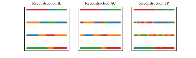
Figure 11: Reconstruction of the problem of Fig. 3, given $n=50$ random points $(x_{i},y_{i})_{i\leq n}$, after loosing at random fifty percent of the coordinates $(\varphi(y_{i}))_{i\leq n}$, leading to sets $(S_{i})_{i\leq n}$ of potential candidates. Hyperparameter were choosen as $\sigma=1$ for the Gaussian kernel and $\lambda=10^{-3}n^{-1/2}$ for the regularization parameter. The percentage of error in the reconstructed Kendall’s embedding is 3% for IL, 4% for AC and 13% for SP. As for classification, with such a random corruption process, AC and IL shows similar behaviors.

B.2.4 Reproducibility specification

To get Fig. 4, we generates eight problems that corresponds to ordering $m=10$ lines, that correspond to eight folds. We only cross validated results with the same heuristics as in Sec. B.1, yet, because computations were expensive we only tried $c_{\sigma}\in\left\{1,.5\right\}$, and $c_{\lambda}\in\left\{10^{3},1,10^{-3}\right\}$. Again, randomness was controlled by instanciating random seeds to 0. Solving the linear program behind our minimum feedback arc set was done using Cplex Cplex, which is the fastest linear program solver we are aware of.

B.3 Multilabel

Multilabel is another application of partial labelling that we did not mention in our experiment section in the core paper. This omission was motivated by the fact that, under natural weak supervision, the three losses (infimum, average and supremum) are basically the same. However, we will provide, now, an explanation of this problem and our algorithm to solve it.

Multilabel prediction consists in finding which are the relevant tags (possibly more than one) among $m$ potential tags. In this case, one can represent $\mathcal{Y}=\left\{-1,1\right\}^{m}$, with $y_{i}=1$ (resp. $y_{i}=-1$), meaning that tag $i$ is relevant (resp. not relevant). The classical loss is the Hamming loss, which is the decoupled sum of errors for each label:

$$\ell(y,z)=\sum_{i=1}^{m}\mathbf{1}_{y_{i}\neq z_{i}}.$$

Natural weak supervision consists in mentioning only a small number of relevant or irrelevant tags. This is the setting of appYu2014. This leads to sets $S$ that are built from a set $P$ of relevant items, and a set $N$ of irrelevant items.

$$S=\left\{y\in\mathcal{Y}\,\middle|\,\forall\,i\in P,y_{i}=1,\forall\,i\in N,y_{i}=-1\right\}.$$

In this case, the infimum loss reads,

$$L(z,S)=\sum_{i\in P}\mathbf{1}_{z_{i}=-1}+\sum_{i\in N}\mathbf{1}_{z_{i}=1}.$$

For such supervision, the infimum, the average and the supremum loss are intrinsically the same, they only differs by constants, due to the fact that for each unseen labels, the infimum loss pays $0$, the average loss $1/2$ and the supremum loss $1$.

When considering data $(x_{i},S_{i})_{i\leq n}$, where $(S_{i})$ is built from $(N_{i},P_{i})$, our algorithm in Eq. 7 reads $\hat{f}(x)=(\operatorname{sign}(\hat{f}_{j}(x)))_{j\leq m}$, based on the scores

$$\hat{f}_{j}(x)=\sum_{i;j\in P_{i}}\alpha_{i}(x)-\sum_{i;j\in N_{i}}\alpha_{i}(x).$$

B.3.1 Tackling positive bias.

In the precedent development, we implicitly assumed that the ratio between positive and negative labels given by the weak supervision reflects the one of the full distribution. An assumptions that is often violated in practice. It is common that partial labelling only mention subset of the revelant tags (i.e., $N=\emptyset$). This case is ill-conditioned as always outputting all tags ($y=\textbf{1}$) will minimize the infimum loss. To solve this problem, we can constrained the prediction space to the top-$k$ space $\mathcal{Y}_{k}=\left\{y\in\mathcal{Y}\,\middle|\,\sum_{i=1}^{m}\mathbf{1}_{y_{j}=1}=k\right\}$, which will lead to taking the top-$k$ over the score $(\hat{f}_{j})_{j\leq m}$. We can also break the loss symmetry and add a penalization with $\varepsilon>0$,

$$\ell_{\varepsilon}(z,y)=\ell(z,y)+\varepsilon\sum_{i=1}^{m}\mathbf{1}_{z_{i}=1}.$$

In this case, the inference algorithm will threshold scores at $\varepsilon$ rather than $0$.

$$f(x)=\left(\operatorname{sign}\left(\sum_{i;j\in P_{i}}\alpha_{i}(x)-\sum_{i;j\in N_{i}}\alpha_{i}(x)\right)\right)_{j\leq m}.$$

B.3.2 Complexity analysis

The complexity analysis is similar to the one for classification. At training, we compute $L=(\mathbf{1}_{j\in P_{i}}-\mathbf{1}_{j\in N_{i}})$ and we solve for $\beta=K_{\lambda}^{-1}L$ in $\mathbb{R}^{n\times m}$. At testing, we compute $v(x)$ and $\beta^{T}v(x)$ in $\mathbb{R}^{m}$, before thresholding it or taking the top-$k$ in either ${\cal O}(m)$ or ${\cal O}(m\log(m))$. As such, complexity reads similarly as for the classification case. Yet notice that, for multilabelling, the dimension of $\mathcal{Y}$ is not $m$ but $2^{m}$, meaning we do not scale with $\#\mathcal{Y}$ but with the intrisic dimension.

Table 3: Complexity of our algorithm for multilabels.

Complexity	Time	Space
Training	${\cal O}(n^{2}(n+m))$	${\cal O}(n(n+m))$
Inference	${\cal O}(nm)$	${\cal O}(n+m)$
Inference top-$k$	${\cal O}(nm+m\log(m))$	${\cal O}(n+m)$

B.3.3 Corruptions on the MULAN datasets

When set comes with tag of few positive and negative tags, all losses are the same. Yet, under other type of supervision, such as when the sets comes as Hamming balls, defined by

$$B(z,r)=\left\{y\in\mathcal{Y}\,\middle|\,\ell(z,y)\leq r\right\},$$

the methods will not behave the same. We experiment on MULAN datasets provided by appTsoumakas2011. Because supervision with Hamming balls does not lead to efficient implementation, we went for extensive grid search for the best solution, which reduce our hability to consider large $m$. Among MULAN datasets, we went for the “scene” one, with $m=6$ tags, and $n=2407$ data. When given a pair $(x,y)$, we add corruption on $y$, by first sampling a radius parameter $r\sim\mathcal{U}\left((\right)[0,c*(m+1)])$, with $c$ a corruption parameter. We then sample, with replacement, $\left\lfloor r\right\rfloor$ coordinates to modify to pass from $y$ to a center $c$. We then consider the supervision $S=B(c,r)$. For such random, somehow uniform, corruption the infimum loss works slightly better than the average loss that both outperform the supremum loss as shown on Fig. 12.

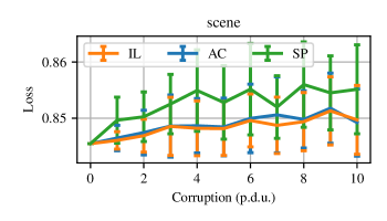
Figure 12: Multilabelling. Testing risks (from Eq. 1) achieved by AC and IL on the “scene” dataset from MULAN as a function of corruption parameter c, shown in procedure defined unit, when the supervision is given as Hamming balls, as described in Sec. B.3.3.

B.3.4 Reproducibility specification

To get Fig. 12, we follow the same cross-validation scheme as for classification and ranking. More exactly, we cross-validated over eight folds with the same heuristics for $\sigma$, the Gaussian kernel parameter, and $\lambda$, the regularization one, with $c_{\sigma}\in\left\{10,5,1,.5,.1,.01\right\}$, and $c_{\lambda}\in\left\{10^{i}\,\middle|\,i\in\left\llbracket-3,3\right\rrbracket\right\}$.

B.4 Partial regression

Partial regression is the regression instance of partial labelling. When supervision comes as interval, it is known as interval regression, and known as censored regression, when sets come as half-lines. Note that for censored regression, nor the average, nor the supremum loss can be properly defined.

B.4.1 Baselines

Given a bounded set $S$, learning with the average loss correspond to considering the center of this set, since, for $z\in\mathcal{Y}$, with $\lambda$ the Lebesgue measure

$$L_{\textit{ac}}(z,S) =\frac{1}{\lambda(S)}\int_{S}\left\|z-y\right\|^{2}\lambda(\mathop{}\!\mathrm{d}y)=\left\|z\right\|^{2}-2\left\langle z,\frac{1}{\lambda(S)}\int_{S}y\lambda(\mathop{}\!\mathrm{d}y)\right\rangle+\frac{1}{\lambda(S)}\int_{S}\left\|y\right\|^{2}\lambda(\mathop{}\!\mathrm{d}y)$$

$$=\left\|z-\frac{1}{\lambda(S)}\int_{S}y\lambda(\mathop{}\!\mathrm{d}y)\right\|^{2}+\frac{1}{\lambda(S)}\int_{S}\left\|y\right\|^{2}\lambda(\mathop{}\!\mathrm{d}y)-\left\|\frac{1}{\lambda(S)}\int_{S}y\lambda(\mathop{}\!\mathrm{d}y)\right\|^{2}=\left\|z-c(S)\right\|^{2}+C_{S},$$

where $c(S)=\frac{1}{\lambda(S)}\int_{S}y\lambda(\mathop{}\!\mathrm{d}y)$ is the center of $S$. As such, the average loss is always convex. As the supremum of convex function, the supremum loss is also convex.

B.4.2 Reproducibility specification

To compute Fig. 5, for both AC and IL, we consider $\sigma$, the Gaussian kernel parameter, and $\lambda$, the regularization parameter, achieving the best risk when measure with the fully supervised distribution, Eq. 1. We tried over $\sigma\in\left\{1,.5,.1,.05,.01\right\}$ and $\lambda\in\left\{10^{3},1,10^{-3}\right\}$. Randomness was controlled by instanciating random seeds.

B.5 Beyond

Beyond the examples showcased precedently, advances in dealing with weak supervision could be beneficial for several problems. Supervision on image segmentation problems usually comes as partial pixel annotation. This problem is often tackled through conditional random fields appVerbeek2007, making it a perfect mix between partial labelling and structured prediction. Action retrieval on instructional video, where partial supervision is retrieved from the audio track is an other interesting application appAlayrac2018.

Minimum feedback arc set

B.6 Formulation

Consider a directed weighted graph with vertex $\left\llbracket 1,m\right\rrbracket$ and edges $\left\{i\rightarrow j\right\}$ with weights $(w_{ij})_{i,j\leq m}\in\mathbb{R}_{+}^{m^{2}}$. The goal is to find directed acyclic graph $G=(V,E)$ that maximize the weights on remaining edges

$$\operatorname*{arg\,max}_{E}\sum_{i\rightarrow j\in E}w_{ij}.$$

This directed acyclic graph can be seen as a preference graph, item $j$ being preferred over item $i$. Since $w_{ij}$ are non-negative, the underlying ordering in $G$ is necessarily total, and therefore can be written based on a score function, that can be embedded in the permutation of $\left\llbracket 1,m\right\rrbracket$, $\sigma\in\mathfrak{S}_{m}$, with $\sigma(j)>\sigma(i)$ meaning that $j$ is preferred over $i$. Thus the problem reads equivalently

$$\operatorname*{arg\,max}_{\sigma\in\mathfrak{S}_{m}}\sum_{i,j\leq m}w_{ij}\mathbf{1}_{\sigma(j)>\sigma(i)} =\operatorname*{arg\,max}_{\sigma\in\mathfrak{S}_{m}}\sum_{i<j\leq m}c_{ij}\mathbf{1}_{\sigma(j)>\sigma(i)}=\operatorname*{arg\,max}_{\sigma\in\mathfrak{S}_{m}}\sum_{i<j\leq m}c_{ij}\operatorname{sign}\left(\sigma(j)-\sigma(i)\right)$$

$$=\operatorname*{arg\,min}_{\sigma\in\mathfrak{S}_{m}}\sum_{i<j\leq m}c_{ij}\operatorname{sign}\left(\sigma(i)-\sigma(j)\right)=\operatorname*{arg\,min}_{\sigma\in\mathfrak{S}_{m}}\sum_{i<j\leq m}c_{ij}\mathbf{1}_{\sigma(i)>\sigma(j)}$$

with $c_{ij}=w_{ij}-w_{ji}$. This last formulation is the one usually encounter for ranking algorithms in machine learning appDuchi2010.

We are going to study in depth this problem under the formulation

$$\operatorname*{arg\,min}_{\sigma\in\mathfrak{S}_{m}}\sum_{i<j\leq m}c_{ij}\operatorname{sign}\left(\sigma(i)-\sigma(j)\right)$$ (9)

B.7 Integer linear programming

Definition 4 (Kendall’s embedding).

For $\sigma\in\mathfrak{S}_{m}$, define Kendall’s embedding, with $m_{e}=m(m-1)/2$,

$$\varphi(\sigma)=\operatorname{sign}\left(\sigma(i)-\sigma(j)\right)_{i<j\leq m}\in\left\{-1,1\right\}^{m_{e}}.$$

Let’s associate to it Kendall’s polytope of order $m$, $\operatorname{Conv}\left(\varphi(\mathfrak{S}_{m})\right)$.

The Kendall’s embedding Def. 4 cast the minimum feedback arcset problem Eq. 9 as a linear program

$$\begin{array}[]{rl}\text{minimize }&\left\langle c,x\right\rangle\\ \text{subject to }&x\in\operatorname{Conv}\left(\varphi(\mathfrak{S}_{m})\right).\end{array}$$

Since the objective is linear, the solution is known to lie on a vertex of the constraint polytope, which is the set of Kendall’s embeddings of permutations. Yet, how to describe Kendall’s polytope?

Definition 5 (Transitivity polytope).

The transitivity polytope of order $m$ is defined in $\mathbb{R}^{m_{e}}$ as

$${\cal M}=\left\{x\in\mathbb{R}^{m_{e}}\,\middle|\,\forall\,i<k<j;-1\leq x_{ij}+x_{jk}-x_{ik}\leq 1\right\}$$

This polytope encodes the transitivity constraints of Kendall’s embeddings Def. 4.

The transitivity polytope Def. 6 will be used to approximate Kendall’s polytope based on the following property.

Proposition 4 (Relaxed polytope).

The intersection between the transitivity polytope and the vertex of the hypercube is exactly the set of Kendall’s embeddings of permutations. Mathematically

$$\varphi(\mathfrak{S}_{m})={\cal M}\cap\left\{-1,1\right\}^{m_{e}}.$$

Proof.

First of all it is easy to show that $\varphi(\mathfrak{S}_{m})\subset\left\{-1,1\right\}^{m_{e}}$, and that, $\varphi(\mathfrak{S}_{m})\subset{\cal M}$.

Let’s now consider $x\in{\cal M}\cap\left\{-1,1\right\}^{m_{e}}$. Let’s associate to $x$ the symmetric embedding

$$\tilde{x}_{ij}=\left\{\begin{array}[]{ccc}x_{ij}&\text{if}&i<j\\ 0&\text{if}&i=j\\ -x_{ji}&\text{if}&j<i\end{array}\right.$$

Let’s consider the permutation $\sigma$ resulting from the ordering of $\sum_{k}\tilde{x}_{ik}$

$$\sigma^{-1}(1)=\operatorname*{arg\,min}_{i\in\left\llbracket 1,m\right\rrbracket}\sum_{k=1}^{m}\tilde{x}_{ik}\qquad\text{and}\qquad\sigma^{-1}(i)=\operatorname*{arg\,min}_{i\in\left\llbracket 1,m\right\rrbracket\backslash\sigma^{-1}\left(\left\llbracket 1,i-1\right\rrbracket\right)}\sum_{k=1}^{m}\tilde{x}_{ik}.$$

Let’s now show that $\varphi(\sigma)=x$, or equivalently that $\tilde{\varphi}(\sigma)=(\operatorname{sign}(\sigma(i)-\sigma(j)))_{i,j\leq m}=\tilde{x}$. First, one can show that $\tilde{x}$ verify the transitivity constraints

$$\forall\,i,j,k\leq m,\qquad-1\leq\tilde{x}_{ij}+\tilde{x}_{jk}-\tilde{x}_{ik}\leq 1.$$

This can be proven for any ordering of $i,j,k$ based on the fact that $x\in{\cal M}$. For example, if $i<k<j$, we have

$$\left[-1,1\right]\ni x_{ik}+x_{kj}-x_{ij}=\tilde{x}_{ik}-\tilde{x}_{jk}-\tilde{x}_{ij}.$$

which leads to

$$\tilde{x}_{ij}+\tilde{x}_{jk}-\tilde{x}_{ik}\in-\left[-1,1\right]=\left[-1,1\right].$$

Now suppose, without loss of generality, that $\tilde{x}_{ij}=1$ (if $\tilde{x}_{ij}=-1$, just consider $\tilde{x}_{ji}=1$). The transitivity constraints tells us that $\tilde{x}_{ik}\geq\tilde{x}_{jk}$ for all $k$, therefore

$$\sum_{k\not\in\left\{i,j\right\}}\tilde{x}_{ik}\geq\sum_{k\not\in\left\{i,j\right\}}\tilde{x}_{jk},\qquad\Rightarrow\qquad\sum_{k=1}^{m}\tilde{x}_{ik}>\sum_{k=1}^{m}\tilde{x}_{jk}.\qquad\Rightarrow\qquad\sigma(i)>\sigma(j).$$

This shows that $\tilde{\varphi(\sigma)}_{ij}=1=\tilde{x}_{ij}$. Thus we have shown that $x\in\varphi(\mathfrak{S}_{m})$, which concludes the proof. ∎

Definition 6 (ILP relaxation).

Based on Prop. 4, we define the canonical polytope ${\cal C}={\cal M}\cap\left[-1,1\right]^{m_{e}}$, and relax the problem Eq. 9 into

$$\begin{array}[]{rl}\text{minimize }&\left\langle c,x\right\rangle\\ \text{subject to }&x\in{\cal C}\end{array}$$

As soon as the solution $x$ is in $\left\{-1,1\right\}^{m_{e}}$, Prop. 4 tells us that $x$ recover the exact minimum feedback arc set solution Eq. 9.

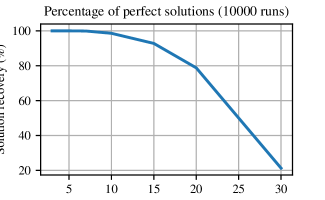
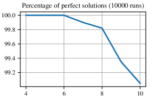
Figure 13: Evaluating the percentage of exact solutions of the ILP relaxation as $m$ grows large. Evaluation is done by choosing a objective $c\sim{\cal N}(0,I_{m_{e}})$, solving the ILP relaxation Def. 6, and evaluating if the solution is in $\left\{-1,1\right\}^{m_{e}}$. The experience is repeated several time to estimate how often, on average, the original solution of Eq. 9 is returned by the ILP.

In small dimension, the canonical polytope ${\cal C}$ is the same as the Kendall’s one, and the ILP relaxation gives the right solution. Yet, as shown Fig. 13, as soon as $m>5$, there exists vertex in ${\cal C}$ that does not correspond to a permutation embedding. For small dimensions, proving that ${\cal C}$ is exactly the Kendall’s polytope is done with a simple drawing for $m=3$, using unimodularity of the transitivity constraint matrix is enough for $m=4$ appHoffman2010. The case $m=5$ is also provable, based on several twicks that we will not discuss here.

Remark (Low noise consistency).

Remark that the low-noise setting considered by appDuchi2010 correspond to having $\operatorname{sign}(c)=-\varphi(y)$ for a $y\in\mathcal{Y}$, in this case our algorithm is consistent and does recover the best solution $z=y$.

B.8 Sorting heuristics

When formatting and solving the integer linear program takes too much time, one can go for simple sorting heuristic, mainly based on a heuristic to compare items two by two and using quick sorting. A review of some heuristic with guarantees is provide by appAilon2005, Similar study when in presence of constraint on the resulting total order can be found in appVanZuylen2007.

appendix/appendix style/icml2020

References

- Ailon et al. (2005) Ailon, N., Charikar, M., and Newman, A. Aggregating inconsistent information: ranking and clustering. In 37th Symposium on Theory of Computing, 2005.
- Arrow (1950) Arrow, K. J. A difficulty in the concept of social welfare. Journal of Political Economy, 58, 1950.
- Bach & Harchaoui (2007) Bach, F. R. and Harchaoui, Z. DIFFRAC: a discriminative and flexible framework for clustering. In Neural Information Processing Systems 20, 2007.
- Bartlett et al. (2006) Bartlett, P. L., Jordan, M. I., and McAuliffe, J. D. Convexity, classification, and risk bounds. Journal of the American Statistical Association, 101, 2006.
- Bengio et al. (2006) Bengio, Y., Delalleau, O., and Roux, N. L. Label propagation and quadratic criterion. In Semi-Supervised Learning. The MIT Press, 2006.
- Caponnetto & De Vito (2006) Caponnetto, A. and De Vito, E. Optimal rates for the regularized least-squares algorithm. Foundations of Computational Mathematics, 7, 2006.
- Chang & Lin (2011) Chang, C. and Lin, C. LIBSVM: A library for support vector machines. ACM TIST, 2, 2011.
- Chapelle et al. (2006) Chapelle, O., Schölkopf, B., and Zien, A. (eds.). Semi-Supervised Learning. The MIT Press, 2006.
- Cid-Sueiro et al. (2014) Cid-Sueiro, J., García-García, D., and Santos-Rodríguez, R. Consistency of losses for learning from weak labels. Lecture Notes in Computer Science, 2014.
- Ciliberto et al. (2016) Ciliberto, C., Rosasco, L., and Rudi, A. A consistent regularization approach for structured prediction. In Neural Information Processing Systems 29, 2016.
- Cour et al. (2011) Cour, T., Sapp, B., and Taskar, B. Learning from partial labels. Journal of Machine Learning Research, 12, 2011.
- Dawid & Skene (1979) Dawid, A. P. and Skene, A. M. Maximum likelihood estimation of observer error-rates using the em algorithm. Applied Statistics, 28, 1979.
- Denoeux (2013) Denoeux, T. Maximum likelihood estimation from uncertain data in the belief function framework. IEEE Transactions on Knowledge and Data Engineering, 25, 2013.
- Duchi et al. (2010) Duchi, J. C., Mackey, L. W., and Jordan, M. I. On the consistency of ranking algorithms. In 27th International Conference on Machine Learning, 2010.
- Fernandes & Brefeld (2011) Fernandes, E. and Brefeld, U. Learning from partially annotated sequences. In Joint European Conference on Machine Learning and Knowledge Discovery in Databases, 2011.
- Grandvalet (2002) Grandvalet, Y. Logistic regression for partial labels. In 9th Information Processing and Management of Uncertainty, 2002.
- Guillaume et al. (2017) Guillaume, R., Couso, I., and Dubois, D. Maximum likelihood with coarse data based on robust optimisation. In 10th International Symposium on Imprecise Probability, 2017.
- Hüllermeier (2014) Hüllermeier, E. Learning from imprecise and fuzzy observations: Data disambiguation through generalized loss minimization. International Journal of Approximate Reasoning, 55, 2014.
- Hüllermeier & Cheng (2015) Hüllermeier, E. and Cheng, W. Superset learning based on generalized loss minimization. In Joint European Conference on Machine Learning and Knowledge Discovery in Databases, 2015.
- Hüllermeier et al. (2008) Hüllermeier, E., Fürnkranz, J., Cheng, W., and Brinker, K. Label ranking by learning pairwise preferences. Artificial Intelligence, 172, 2008.
- Jin & Ghahramani (2002) Jin, R. and Ghahramani, Z. Learning with multiple labels. In Neural Information Processing Systems 15, 2002.
- Joulin et al. (2010) Joulin, A., Bach, F. R., and Ponce, J. Discriminative clustering for image co-segmentation. In 23th Conference on Computer Vision and Pattern Recognition, 2010.
- Kemeny (1959) Kemeny, J. G. Mathematics without numbers. Daedalus, 88, 1959.
- Kendall (1938) Kendall, M. G. A new measure of rank correlation. Biometrika, 30, 1938.
- Korba et al. (2018) Korba, A., Garcia, A., and d’Alché-Buc, F. A structured prediction approach for label ranking. In Neural Information Processing Systems 31, 2018.
- Lafferty et al. (2001) Lafferty, J. D., McCallum, A., and Pereira, F. C. N. Conditional random fields: Probabilistic models for segmenting and labeling sequence data. In 18th International Conference on Machine Learning, 2001.
- Luo & Orabona (2010) Luo, J. and Orabona, F. Learning from candidate labeling sets. In Neural Information Processing Systems 23, 2010.
- Madry et al. (2018) Madry, A., Makelov, A., Schmidt, L., Tsipras, D., and Vladu, A. Towards deep learning models resistant to adversarial attacks. In 6th International Conference on Learning Representations, 2018.
- Mayhew et al. (2019) Mayhew, S., Chaturvedi, S., Tsai, C., and Roth, D. Named entity recognition with partially annotated training data. In 23rd Conference on Computational Natural Language Learning, 2019.
- Micchelli et al. (2006) Micchelli, C. A., Xu, Y., and Zhang, H. Universal kernels. Journal of Machine Learning Research, 7, 2006.
- Muandet et al. (2017) Muandet, K., Fukumizu, K., Sriperumbudur, B. K., and Schölkopf, B. Kernel mean embedding of distributions: A review and beyond. Foundations and Trends in Machine Learnig, 10, 2017.
- Nguyen & Caruana (2008) Nguyen, N. and Caruana, R. Classification with partial labels. In 14th International Conference on Knowledge Discovery and Data Mining, 2008.
- Nowak-Vila et al. (2019) Nowak-Vila, A., Bach, F., and Rudi, A. Sharp analysis of learning with discrete losses. In 22nd International Conference on Artificial Intelligence and Statistics, 2019.
- Papandreou et al. (2015) Papandreou, G., Chen, L., Murphy, K. P., and Yuille, A. L. Weakly-and semi-supervised learning of a deep convolutional network for semantic image segmentation. In International Conference on Computer Vision, 2015.
- Quadrianto et al. (2009) Quadrianto, N., Smola, A. J., Caetano, T. S., and Le, Q. V. Estimating labels from label proportions. Journal of Machine Learning Research, 10, 2009.
- Scholkopf & Smola (2001) Scholkopf, B. and Smola, A. J. Learning with kernels: support vector machines, regularization, optimization, and beyond. MIT press, 2001.
- Smale & Zhou (2007) Smale, S. and Zhou, D.-X. Learning theory estimates via integral operators and their approximations. Constructive Approximation, 26, 2007.
- Tobin (1958) Tobin, J. Estimation of relationships for limited dependent variables. Econometrica, 26, 1958.
- Tsochantaridis et al. (2005) Tsochantaridis, I., Joachims, T., Hofmann, T., and Altun, Y. Large margin methods for structured and interdependent output variables. Journal of Machine Learning Research, 6, 2005.
- van Rooyen & Williamson (2017) van Rooyen, B. and Williamson, R. C. A theory of learning with corrupted labels. Journal of Machine Learning Research, 18, 2017.
- van Zuylen et al. (2007) van Zuylen, A., Hegde, R., Jain, K., and Williamson, D. P. Deterministic pivoting algorithms for constrained ranking and clustering problems. In 18th Symposium on Discrete Algorithms, 2007.
- Verbeek & Triggs (2008) Verbeek, J. and Triggs, W. Scene Segmentation with CRFs Learned from Partially Labeled Images. In Neural Information Processing Systems 20, 2008.
- Wald (1945) Wald, A. Statistical decision functions which minimize the maximum risk. The Annals of Mathematics, 46, 1945.
- Weiss (1999) Weiss, Y. Segmentation using eigenvectors: a unifying view. 7th International Conference on Computer Vision, 1999.
- Xu et al. (2004) Xu, L., Neufeld, J., Larson, B., and Schuurmans, D. Maximum margin clustering. In Neural Information Processing Systems, 2004.
- Yu et al. (2014) Yu, H., Jain, P., Kar, P., and Dhillon, I. S. Large-scale multi-label learning with missing labels. In 31th International Conference on Machine Learning, 2014.
- Zhou et al. (2003) Zhou, D., Bousquet, O., Lal, T. N., Weston, J., and Schölkopf, B. Learning with local and global consistency. In Neural Information Processing Systems 16, 2003.
- Zhu et al. (2003) Zhu, X., Ghahramani, Z., and Lafferty, J. D. Semi-supervised learning using gaussian fields and harmonic functions. In 20th International Conference of Machine Learning, 2003.