$B_{c}\to B_{s(d)}$ form factors from lattice QCD

Abstract

We present results of the first lattice QCD calculations of $B_{c}\to B_{s}$ and $B_{c}\to B_{d}$ weak matrix elements. Form factors across the entire physical $q^{2}$ range are then extracted and extrapolated to the physical-continuum limit before combining with CKM matrix elements to predict the semileptonic decay rates $\Gamma(B_{c}^{+}\to B_{s}^{0}\overline{\ell}\nu_{\ell})=26.2(1.2)\times 10^{9}\hskip 2.84526pt\text{s}^{-1}$ and $\Gamma(B_{c}^{+}\to B^{0}\overline{\ell}\nu_{\ell})=1.65(10)\times 10^{9}\hskip 2.84526pt\text{s}^{-1}$. The lattice QCD uncertainty is comparable to the CKM uncertainty here. Results are derived from correlation functions computed on MILC Collaboration gauge configurations with a range of lattice spacings including 2+1+1 flavours of dynamical sea quarks in the Highly Improved Staggered Quark (HISQ) formalism. HISQ is also used for the propagators of the valence light, strange, and charm quarks. Two different formalisms are employed for the bottom quark: non-relativistic QCD (NRQCD) and heavy-HISQ. Checking agreement between these two approaches is an important test of our strategies for heavy quarks on the lattice. From chained fits of NRQCD and heavy-HISQ data, we obtain the differential decay rates $d\Gamma/dq^{2}$ as well as integrated values for comparison to future experimental results.

I Introduction

The semileptonic weak decays $B_{c}^{+}\to B_{s}^{0}\overline{\ell}\nu_{\ell}$ and $B_{c}^{+}\to B^{0}\overline{\ell}\nu_{\ell}$ proceed via tree-level flavour changing processes $c\to sW^{+}$ and $c\to dW^{+}$ parametrised by the Cabbibo-Kobayashi-Maskawa (CKM) matrix of the Standard Model. Associated weak matrix elements can be expressed in terms of form factors which capture the non-perturbative QCD physics. Precise determination of the normalisation and the $q^{2}$ dependence of these form factors from lattice QCD will allow a novel comparison with future experiment to deduce the CKM parameters $V_{cs}$ and $V_{cd}$. Lattice studies of other semileptonic meson decays that involve tree-level weak decays of a constituent charm quark include Aubin et al. (2005); Na et al. (2010); Koponen et al. (2013); Donald et al. (2014); Bazavov et al. (2014); Lubicz et al. (2017). Precise determination of these CKM matrix elements is critical for examining the second row unitary constraint

$$|V_{cd}|^{2}+|V_{cs}|^{2}+|V_{cb}|^{2}=1.$$ (1)

This will complement other unitarity tests of the CKM matrix. It is possible LHCb could measure $B_{c}^{+}\to B_{s}^{0}\overline{\mu}\nu_{\mu}$ using Run 1 and 2 data. For example, normalising by $B_{c}^{+}\to J/\psi\overline{\mu}\nu_{\mu}$ would yield a constraint on the ratio $V_{cs}/V_{cb}$. Due to CKM suppression, a measurement of $B_{c}^{+}\to B^{0}\overline{\mu}\nu_{\mu}$ is likely to require many more $B_{c}^{+}$ decays.

A lattice study of the $B_{c}^{+}\to B_{s}^{0}\overline{\ell}\nu_{\ell}$ and $B_{c}^{+}\to B^{0}\overline{\ell}\nu_{\ell}$ decays involves the practical complication of a heavy spectator quark. Care must be taken in placing such a particle on the lattice to avoid large discretisation effects. We consider two formalisms for the $b$ quark. A valence NRQCD Lepage et al. (1992); Dowdall et al. (2012) $b$ quark, a formalism constructed from a non-relativistic effective theory, is used to simulate with physically massive $b$ quarks. A complementary calculation uses HPQCD’s heavy-HISQ method McNeile et al. (2010, 2012); McLean et al. (2019). Here, all flavours of quark are implemented with the HISQ Follana et al. (2007) formalism. This is a fully relativistic approach which involves calculations for a set of quark masses on ensembles of lattices with a range of fine lattice spacings, enabling a fit from which the physical result at the $b$ quark mass in the continuum can be determined. The method with an NRQCD bottom quark also uses HISQ for the charm, strange and down flavours. This study will demonstrate the consistency of the NRQCD and heavy-HISQ approaches by comparing the form factors extrapolated to the physical-continuum limit.

In the limit of massless leptons, the differential decay rates for $B_{c}^{+}\to B_{s}^{0}\overline{\ell}\nu_{\ell}$ and $B_{c}^{+}\to B^{0}\overline{\ell}\nu_{\ell}$ are given by

$$\frac{d\Gamma}{dq^{2}}=\frac{G_{F}^{2}|V|^{2}}{24\pi^{3}}|\mathbf{p}_{2}|^{3}|f_{+}(q^{2})|^{2},$$ (2)

where $V$ is the relevant associated CKM matrix element $V_{cs}$ or $V_{cd}$ and $f_{+}$ is one of two form factors that parametrise the continuum weak matrix element

$$\langle B_{s(d)}(\mathbf{p}_{2}) |V^{\mu}|B_{c}(\mathbf{p}_{1})\rangle=f_{0}(q^{2})\Bigg{[}\frac{M_{B_{c}}^{2}-M_{B_{s(d)}}^{2}}{q^{2}}q^{\mu}\Bigg{]}$$

$$+f_{+}(q^{2})\Bigg{[}p_{2}^{\mu}+p_{1}^{\mu}-\frac{M_{B_{c}}^{2}-M_{B_{s(d)}}^{2}}{q^{2}}q^{\mu}\Bigg{]}.$$ (3)

Table 1: Parameters for the MILC ensembles of gluon field configurations. The lattice spacing $a$ is determined from the Wilson flow parameter $w_{0}$ Borsanyi et al. (2012) given in lattice units for each set in column 2 where values were obtained from Chakraborty et al. (2017a) on sets 1 to 5 and Chakraborty et al. (2015) on set 6. The physical value $w_{0}=0.1715(9)$ was fixed from $f_{\pi}$ in Dowdall et al. (2013). Sets 1 and 2 have $a\approx 0.15$ [fm], and sets 3 and 4 have $a\approx 0.12$ [fm]. Sets 5 and 6 have $a\approx 0.09$ [fm] and $a\approx 0.06$ [fm] respectively. Sets 1, 3, 5 and 6 have unphysically massive light quarks such that $m_{l}/m_{s}=0.2$. Sets 1 to 5 were used in the NRQCD calculation of the form factors. The heavy-HISQ calculation used sets 3, 5 and 6.

set	$w_{0}/a$	$N_{x}^{3}\times N_{t}$	$n_{\text{cfg}}$	$am_{l}^{\text{sea}}$	$am_{s}^{\text{sea}}$	$am_{c}^{\text{sea}}$
1	1.1119(10)	$16^{3}\times 48$	$1000$	$0.013$	$0.065$	$0.838$
2	1.1367(5)	$32^{3}\times 48$	$500$	$0.00235$	$0.0647$	$0.831$
3	1.3826(11)	$24^{3}\times 64$	$1053$	$0.0102$	$0.0509$	$0.635$
4	1.4149(6)	$48^{3}\times 64$	$1000$	$0.00184$	$0.0507$	$0.628$
5	1.9006(20)	$32^{3}\times 96$	$504$	$0.0074$	$0.037$	$0.440$
6	2.896(6)	$48^{3}\times 144$	$250$	$0.0048$	$0.024$	$0.286$

Table 2: The HISQ valence quark masses for the light, strange and charm flavours for each of the sets described in Table 1. For the light quarks, the values for the valence quarks are identical to the masses of the light sea quarks. The masses for the valence strange quarks and the valence charm quarks were tuned in Chakraborty et al. (2015) using $w_{0}$ (Table 1) to fix the lattice spacing. The fourth and fifth columns give the valence charm quark masses for the calculations with NRQCD and HISQ spectator quarks respectively. In the calculation with NRQCD spectator quarks slightly different $am_{c}^{\text{val}}$ values were used for historical reasons. Our fits allow for mistuning of the charm quark mass.

			$am_{c}^{\text{val}}$
set	$am_{l}^{\text{val}}$	$am_{s}^{\text{val}}$	NRQCD spectator	HISQ spectator
1	0.013	0.0705	0.826
2	0.00235	0.0677	0.827
3	0.0102	0.0541	0.645	0.663
4	0.00184	0.0507	0.631
5	0.0074	0.0376	0.434	0.450
6	0.0048	0.0234		0.274

The 4-momentum transfer is $q=p_{1}-p_{2}$, and only the vector part of the $V-A$ weak current contributes since QCD conserves parity. The contribution of $f_{0}$ to the decay rate is suppressed by the lepton mass and hence irrelevant for the decays to $e\overline{\nu}_{e}$ and $\mu\overline{\nu}_{\mu}$. The phase space is sufficiently small to disallow decays to $\tau\overline{\nu}_{\tau}$. Form factors are constructed from the matrix elements that are obtained by fitting the appropriate lattice QCD 3-point correlator data. By calculating correlators at a range of transfer momenta on lattices with different spacings and quark masses, continuum form factors at physical quark masses are obtained and then appropriately integrated to offer a direct comparison with decay rates that could be measured in experiment.

In this study, we begin with Sec. II in which details of the lattice calculations are described. Sec. II.1 reports on the parameters and gauge configurations used to generate the propagators. Next, Sec. II.2 explains how the correlators are subsequently constructed for the two different treatments of the heavy spectator quark, as well as how the correlator data is fit to extract the matrix elements. Our non-perturbative renormalisation method required to obtain the form factors is set out in Sec. II.3. Sec. III presents results of the lattice calculations. Correlator fits are examined in Sec. III.1, whilst Sec. III.2 discusses results for the renormalisation of the local lattice vector current. In Sec. III.3, the form factor data for the cases of an NRQCD spectator and a HISQ spectator are plotted alongside. Sec. IV is concerned with the methodology and results from fitting the form factor data. An extrapolation of the form factors to physical-continuum point is presented in Sec. IV.4 and Sec. IV.5 shows how the form factors depend on the mass of the spectator quark. Finally, in Sec. V we give our conclusions.

II Lattice Calculation

II.1 Parameters and Set-up

We use ensembles with $2+1+1$ flavours of HISQ sea quark generated by the MILC Collaboration Bazavov et al. (2010, 2013, 2016) and described in Table 1. The Symanzik-improved gluon action used is that from Hart et al. (2009), where the gluon action is improved perturbatively through $\mathcal{O}(\alpha_{s})$ including the effect of dynamical HISQ sea quarks. The lattice spacing is identified by comparing the physical value for the Wilson flow parameter $\omega_{0}=0.1715(9)$ fm Dowdall et al. (2013) with lattice values for $\omega_{0}/a$ from Chakraborty et al. (2017a) and Chakraborty et al. (2015). Our calculations feature physically massive strange quarks and equal mass up and down quarks, with a mass denoted by $m_{l}$, with $m_{l}/m_{s}=0.2$ and also the physical value $m_{l}/m_{s}=1/27.4$ Bazavov et al. (2014). For sets 1 to 5 in Table 1, strange propagators were re-used from Koponen et al. (2017), a study of the pseudoscalar meson electromagnetic form factor. Light propagators were re-used from Koponen (2016), an extension of Koponen et al. (2017) to the pion. The valence quark masses used for the HISQ propagators on these gluon configurations are given in Table 2. The valence strange and charm quark masses used here were tuned in Chakraborty et al. (2015); Koponen et al. (2017), slightly away from the sea quark masses to yield results that more closely correspond to physical values. The propagators were calculated using the MILC code MIL .

Table 3: The bottom quark masses, NRQCD action parameters $c_{j}$, and values for the tadpole improvement $u_{0}$ were obtained from Dowdall et al. (2012). The final columns gives the different momenta for the strange and light quarks considered in the NRQCD calculation implemented with twisted boundary conditions.

set	$am_{b}^{\text{val}}$	$c_{1},c_{6}$	$c_{5}$	$c_{4}$	$u_{0}$	$|a\mathbf{q}|$
1	$3.297$	$1.36$	$1.21$	$1.22$	$0.8195$	0	0.1243	0.3730	0.6217
2	$3.25$	$1.36$	$1.21$	$1.22$	$0.8195$	0	0.3649
3	2.66	1.31	1.16	1.20	0.8341	0	0.1	0.3	0.5
4	$2.62$	$1.31$	$1.16$	$1.20$	$0.8341$	0
5	$1.91$	$1.21$	$1.12$	$1.16$	$0.8525$	0	0.0728	0.364	0.437

Table 4: Heavy quark masses and momenta used for the heavy-HISQ calculation. The momenta are in the $(1\hskip 2.84526pt1\hskip 2.84526pt1)$ direction.

set	$am_{h}^{\text{val}}$				$|a\mathbf{q}|$
3	0.663	0.8			0	0.1	0.3	0.5
5	0.450	0.6	0.8		0	0.07281	0.218	0.364	0.437
6	0.274	0.450	0.6	0.8	0	0.143	0.239	0.334

We work in the frame where the $B_{c}^{+}$ is at rest, and momentum is inserted into the strange or down valence quark through twisted boundary conditions Sachrajda and Villadoro (2005); Guadagnoli et al. (2006) in the $(1\hskip 2.84526pt1\hskip 2.84526pt1)$ direction. The values of the momenta used are given in Tables 3 and 4. The periodic boundary conditions of the fermion fields are modified by phases $\theta_{i}$

$$\psi(n+N_{x}\hat{i}) =e^{i\pi\theta_{i}}\psi(n)$$ (4)

so that the usual lattice momenta $q_{i}=2\pi k_{i}/aN_{x}$, for integers $k_{i}$, are shifted by $\pi\theta_{i}/aN_{x}$. The corresponding $q^{2}$ is then constructed by taking $q_{0}$ to be the difference in energies of the lowest lying initial and final states.

The coefficients of operators corresponding to relativistic correction terms in the NRQCD action are given in Table 3. The valence $b$ quark masses used for the NRQCD propagators are also given there. The values were taken from Dowdall et al. (2012), where the $b$ quark mass was found by matching the experimental value for the spin-averaged kinetic mass of the $\Upsilon$ and the $\eta_{b}$ to lattice data. For the calculation with an NRQCD spectator bottom quark, we use sets 1 to 5 in Table 1.

Bare heavy quark masses $am_{h}$ used for the heavy-HISQ method are shown in Table 4. The selection of heavy quark masses follows McLean et al. (2019). As well as sets 3 and 5, the heavy-HISQ calculation makes use of a lattice finer than the five sets featuring in the calculation with an NRQCD spectator, set 6 in Table 1. This is motivated by the necessity to avoid large discretisation effects that grow with $(am_{h})$ (as $(am_{h})^{4}$ at tree-level) whilst gathering data at large masses that will reliably inform the limit $m_{h}\to m_{b}$.

II.2 Correlators

II.2.1 NRQCD spectator case

For the case of an NRQCD spectator quark, random wall source Aubin et al. (2004) HISQ propagators with the mass of the charm quark are calculated and combined with random wall source NRQCD $b$ propagators to generate $B_{c}^{+}$ 2-point correlator data. 2-point correlators for $B_{s(d)}^{0}$ are generated similarly. The strategy of combining NRQCD random wall propagators and HISQ random wall propagators to yield 2-point correlators was first developed in Gregory et al. (2011). NRQCD propagators are generated by solving an initial value problem. This is computationally very fast compared to calculating rows of the inverse of the quark matrix.

Figure 1: 3-point correlator $C_{\text{3pt}}(t,T)$. The flavour-changing operator insertion is denoted by a cross at timeslice $t$ and the total time length of the 3-point correlator is $T$. The random wall source for the $b$ and $s/d$ propagators is at the timeslice of the $B_{s(d)}$ interpolator.

The 3-point correlator needed here is represented diagrammatically in Fig. 1. A HISQ charm quark propagator is generated by using the random wall bottom quark propagator as a sequential source. Following Appendix B in Donald et al. (2012), and excluding a spacetime-dependent sign, the sequential source is given by the spin-trace

$$\text{Tr}_{\text{spin}}\Big{\{}\Gamma\Omega^{\dagger}(\mathbf{x},0)S_{b}^{\text{RW}}(\mathbf{x},0)\Big{\}},$$ (5)

where $\Gamma$ is the gamma matrix structure at the operator insertion, $S_{b}^{\text{RW}}$ is the random wall NRQCD propagator, and

$$\Omega(x)\coloneqq \prod_{\mu=1}^{4}(\gamma_{\mu})^{\frac{x_{\mu}}{a}}$$ (6)

is the space-spin matrix which transforms the naive quark field to diagonalise the HISQ action in spin-space.

II.2.2 HISQ spectator case

The case of a HISQ spectator quark proceeds similarly with the only difference being the use of a HISQ propagator instead of an NRQCD propagator for the bottom quark. Again, the charm propagator uses the spectator bottom quark propagator as a sequential source. Multiple masses are used for the spectator quark, each requiring a different charm propagator for the 3-point correlator. Fig. 2 shows the heavy-charm pseudoscalar meson masses that arise from calculations with the $am_{h}$ values in Table 4. On set 6, the finest lattice considered, we reach a value for $M_{H_{c}}$ that is $80\%$ of the physical $B_{c}$ mass.

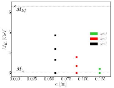
Figure 2: The mass $M_{H_{c}}$ of the heavy-charm meson is plotted against lattice spacing for each of the values of $am_{h}$ used in the heavy-HISQ calculation. Obtained from fitting the correlators as described in Eq. (II.2.3), $M_{H_{c}}$ is a proxy for the bare lattice heavy quark mass $am_{h}$. The continuum-physical point is denoted by a cross at $a=0$ [fm] and $M_{H_{c}}=M_{B_{c}^{+}}$. Note that the $y$-axis scale begins near $M_{\eta_{c}}$.

The same strange and light random wall HISQ propagators on sets 3 and 5 are used in both the NRQCD and the heavy-HISQ calculations, thus the data on these lattices in the two approaches will be correlated. However, the effect of these correlations is small in the physical-continuum limit since the heavy-HISQ data on sets 3 and 5 are the furthest away from the physical $b$ quark mass point, and hence these correlations are safely ignored.

II.2.3 Fitting the correlators

The correlator fits minimise an augmented $\chi^{2}$ function as described in Lepage et al. (2002); Hornbostel et al. (2012); Bouchard et al. (2014). The functional forms for the 2-point and 3-point correlators

$$C^{B_{s(d)}}_{\text{2pt}}(t) =\sum_{i}a[i]^{2}e^{-E_{a}[i]t}-\sum_{i}a_{o}[i]^{2}(-1)^{t}e^{-E_{a_{o}}[i]t}$$

$$C^{B_{c}}_{\text{2pt}}(t) =\sum_{j}b[j]^{2}e^{-E_{b}[j]t}-\sum_{j}b_{o}[j]^{2}(-1)^{t}e^{-E_{b_{o}}[j]t}$$

$$C_{\text{3pt}}(t,T) =\sum_{i,j}a[i]e^{-E_{a}[i]t}V_{nn}[i,j]b[j]e^{-E_{b}[j](T-t)}$$

$$-\sum_{i,j} (-1)^{T-t}a[i]e^{-E_{a}[i]t}V_{no}[i,j]b_{o}[j]e^{-E_{b_{o}}[j](T-t)}$$

$$-\sum_{i,j} (-1)^{t}a_{o}[i]e^{-E_{a_{o}}[i]t}V_{on}[i,j]b[j]e^{-E_{b}[j](T-t)}$$

$$+\sum_{i,j} (-1)^{T}a_{o}[i]e^{-E_{a_{o}}[i]t}V_{oo}[i,j]b_{o}[j]e^{-E_{b_{o}}[j](T-t)}$$

follow from their spectral decomposition and include oscillatory contributions from the staggered quark time-doubler. The matrix elements are related to the fit parameters $V_{nn}[i,j]$ through

$$V_{nn}[0,0]=\frac{\langle B_{s(d)}|J|B_{c}\rangle}{\sqrt{2E_{B_{s(d)}}2E_{B_{c}}}},$$ (8)

where $J$ is the relevant operator that facilitates the $c\to s(d)$ flavour transition. The pseudoscalar mesons of interest are the lowest lying states consistent with their quark content, so we are only concerned with the matrix elements for $i=j=0$ since we restrict $E[k]\leq E[k+1]$ by using log-normal prior distributions for the energy differences. The presence of $i,j>0$ terms are necessary to give a good fit and to allow for the full systematic uncertainty from the presence of excited states to be included in the extracted $V_{nn}[0,0]$. On each set, the 2-point and 3-point correlator data for both $c\to s$ and $c\to d$ at all momenta are fit simultaneously to account for all possible correlations. The matrix elements and energies are extracted and form factor values determined, along with the correlations between results at different momenta.

II.3 Extracting The Form Factors

The Partially Conserved Vector Current (PCVC) Ward identity allows for a fully non-perturbative renormalisation of the lattice vector current. Since the same HISQ action is used for the $c$ and $s(d)$ quarks that couple to the $W^{+}$ in both the NRQCD and heavy-HISQ approaches, we have the PCVC identity

$$\ \partial_{\mu}V^{\mu}_{\text{cons}}=(m_{c}-m_{s(d)})S,$$ (9)

relating the conserved (point-split) $c\to s(d)$ lattice vector current and the local lattice scalar density $S$. We choose a local lattice operator $V^{\mu}_{\text{loc}}$, thus Eq. (9) must be adjusted by a single renormalisation factor $Z_{V}$ associated with that operator, giving

$$q_{\mu}\langle B_{s(d)}|V^{\mu}_{\text{loc}}|B_{c}\rangle Z_{V}=(m_{c}-m_{s(d)})\langle B_{s(d)}|S|B_{c}\rangle.$$ (10)

Since $Z_{V}$ is $q^{2}$ independent, in principle $Z_{V}$ need only be found at zero-recoil where $q^{\mu}$ has only a temporal component Koponen et al. (2013). This avoids the need to calculate 3-point correlators associated with the spatial components of the vector current matrix element that appear in Eq. (10) for $\mathbf{q}\neq\mathbf{0}$. However, in practice, it is preferable to determine $f_{+}$ near zero-recoil through the spatial components of the vector current matrix element, albeit with the additional cost in computing 3-point correlators with the corresponding insertion.

As in Na et al. (2010), we combine Eqs. (I) and (10) to give a determination

$$f_{0}\big{(}q^{2}\big{)}=\langle B_{s(d)}|S|B_{c}\rangle\frac{m_{c}-m_{s(d)}}{M_{B_{c}}^{2}-M_{B_{s(d)}}^{2}}$$ (11)

of $f_{0}$ solely in terms of the scalar density matrix element. We use Eq. (11) and calculation of the vector current matrix element to determine $f_{+}$ and $f_{0}$ for the full $q^{2}$ range following  Koponen et al. (2013); Chakraborty et al. (2018). Thus, we will calculate matrix elements of both the local scalar density $J=S$ and the local vector current $J=V$.

Once $f_{0}$ is determined, $f_{+}$ is obtained using Eq. (I) for $\mu=0$ to yield

$$f_{+}(q^{2})=\frac{Z_{V}\mathcal{V}^{0}-q^{0}f_{0}(q^{2})\frac{M_{B_{c}^{+}}^{2}-M_{B_{s}^{0}}^{2}}{q^{2}}}{p_{2}^{0}+p_{1}^{0}-q^{0}\frac{M_{B_{c}^{+}}^{2}-M_{B_{s}^{0}}^{2}}{q^{2}}},$$ (12)

where $\mathcal{V}^{\mu}$ is the vector current matrix element, except at zero-recoil where the denominator vanishes and $f_{+}$ cannot be extracted. We find that using Eq. (12) near zero-recoil is problematic since both the numerator and denominator grow from 0 as $q^{2}$ is decreased from the maximum value at zero-recoil. For the case where the spectator is an NRQCD $b$ quark, we instead use Eq. (I) with $\mu=i\neq 0$

$$f_{+}(q^{2}) =\frac{-\frac{Z_{V}\mathcal{V}^{i}}{q^{i}}+f_{0}(q^{2})\frac{M_{B_{c}^{+}}^{2}-M_{B_{s}^{0}}^{2}}{q^{2}}}{1+\frac{M_{B_{c}^{+}}^{2}-M_{B_{s}^{0}}^{2}}{q^{2}}}.$$ (13)

This method gives much smaller errors near to zero-recoil. Although mathematically equivalent to Eq. (12), extracting $f_{+}$ through Eq. (13) does not suffer an inflation of error near zero-recoil since both the numerator and denominator are non-zero for all physical $q^{2}$. However, since $\mathcal{V}^{i}$ appears explicitly in Eq. (13), 3-point correlators with an insertion of $V^{i}$ need to be calculated. For the case of the spectator NRQCD $b$ quark, the use of Eq. (13) is straightforward except that it requires inversions of the charm quark propagator from a different sequential source (see Eq. (5)) to allow for insertion of the current $V^{i}=\gamma^{i}\otimes\gamma^{i}$ in the mixed NRQCD-HISQ 3-point function. Collecting $\mathcal{V}^{i}$ at non-zero 3-momentum transfer in the NRQCD calculation will also test for any $q^{2}$ dependence of $Z_{V}$ that would appear as a discretisation effect.

Using Eqs. (11) and (12) or (13), form factor data at a variety of lattice spacings, light quark masses and momenta are obtained from the energies and matrix elements.

II.3.1 NRQCD spectator case

For the case of an NRQCD spectator quark, the form factor extraction is complicated by the energy offset as a consequence of the subtraction of the $b$ quark rest mass inherent in the NRQCD formalism. Whilst physical energy differences are preserved with NRQCD quarks, energy sums are not. Consequently, Particle Data Group (PDG) Tanabashi et al. (2018) values are used where necessary. For example, we take

$$M_{B_{c}}^{2}-M_{B_{s}(d)}^{2} =\Big{(}E^{\text{sim}}_{B_{c}}(|a\mathbf{q}|=0)-E^{\text{sim}}_{B_{s(d)}}(|a\mathbf{q}|=0)\Big{)}$$

$$\hskip 42.67912pt\times\Big{(}M_{B_{c}}^{\text{PDG}}+M_{B_{s}(d)}^{\text{PDG}}\Big{)}$$ (14)

when extracting the form factors. We use interpolating operators $\overline{c}\gamma_{5}b$ and $\overline{s}\gamma_{5}b$ ($\overline{d}\gamma_{5}b$) for $J^{P}=0^{-}$ pseudoscalars $B_{c}^{+}$ and $B_{s(d)}^{0}$ respectively.

II.3.2 HISQ spectator case

For the case of a HISQ spectator quark, we work only with local scalar and vector currents. Expressed in the spin-taste basis, we use $\gamma_{5}\otimes\gamma_{5}$ for the $H_{s(d)}$ interpolating operator and two different operators, $\gamma_{5}\otimes\gamma_{5}$ and $\gamma_{5}\gamma_{0}\otimes\gamma_{5}\gamma_{0}$, for the $H_{c}$ interpolator. The first of these, $\gamma_{5}\otimes\gamma_{5}$, makes a tasteless 3-point correlation function when the scalar density operator $\mathbb{1}\otimes\mathbb{1}$ is used. The second, $\gamma_{5}\gamma_{0}\otimes\gamma_{5}\gamma_{0}$, allows for a tasteless 3-point correlation function when we use the local temporal vector current operator $\gamma_{0}\otimes\gamma_{0}$ Koponen et al. (2013). This requires the calculation of two $H_{c}$ 2-point functions with the two different choices of operator at both the source and the sink. The difference in masses between these two different tastes of $H_{c}$ meson is tiny and, although consistently taken care of, it has no impact on the calculation.

III Results

III.1 Correlators

Figs. 3 and 4 provide samples of the correlator data from the NRQCD and heavy-HISQ calculations respectively. The quantity plotted is the effective simulation energies, which we define by the two-step log-ratio

$$aE_{\text{sim,eff}} =\frac{1}{2}\log\Big{(}\frac{C(t)}{C(t+2)}\Big{)}.$$ (15)

This ratio is preferable to an effective energy defined using $C(t)/C(t+1)$ since the ratio in Eq. (15) better suppresses the oscillatory contributions in Eq. (II.2.3). Error bars are present in the figure but mostly too small to observe. We exclude $t_{\text{min}}/a$ data points from the beginning and end points of the correlators in our fits to reduce the contributions from excited states.

Figure 3: Effective simulation energies (Eq. (15)) of 2-point correlators with an NRQCD spectator quark on set 5 for $|a\mathbf{q}|=0.427$. The black lines with grey error bands show the energies extracted from fitting the correlators in the simultaneous fit of fine lattice data with all the 3-point correlators and all the momenta. The $B$ meson energies shown here are offset from their physical values as a consequence applying the NRQCD formalism to the constituent $b$ quark.

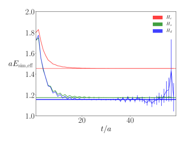
Figure 4: Effective simulation energies (Eq. (15)) of 2-point correlators with a HISQ spectator quark on set 6 at zero twist with $am_{h}=0.8$. The horizontal bands show the energies extracted from the full simultaneous correlator fit.

For each of the cases of an NRQCD and HISQ spectator quark, we fit all of the correlator data to Eq. (II.2.3) on each set simultaneously to obtain the correlations between the fitted parameters. Consequently, the correlator fits involve a large covariance matrix. Without extremely large statistical samples of results small eigenvalues of the covariance matrix are underestimated Michael (1994); Dowdall et al. (2019) and this causes problems when carrying out the inversion to find $\chi^{2}$. We overcome this by using an SVD (singular-value decomposition) cut; any eigenvalue of the covariance matrix smaller than some proportion $c$ of the biggest eigenvalue $\lambda_{\text{max}}$ is replaced by $c\lambda_{\text{max}}$. By carrying out this procedure, the covariance matrix becomes less singular. These eigenvalue replacements will only inflate our final errors, hence this strategy is conservative. The SVD cut reduces the $\chi^{2}/$d.o.f. reported by the fit because it lowers the contribution to $\chi^{2}$ of the modes with eigenvalues below the SVD cut. In order to check the suitability of the SVD cut, we must test the goodness-of-fit from a fit where noise (SVD-noise) is added to the data to reinstate the size of fluctuations expected from the modes below SVD cut, as described in Appendix D of Dowdall et al. (2019). The $\chi^{2}_{\text{SVD-noise}}/$d.o.f. is used to check the goodness of fit for both cases of spectator quark.

Many fits were carried out with different SVD cuts, number of exponentials $N$, and positions $t_{\text{min}}^{\text{2pt}}$ and $t_{\text{min}}^{\text{3pt}}$ of the first timeslice where the correlators are fit. We selected the fit of the correlators on each lattice for form factor extraction based on the $\chi^{2}/\text{d.o.f.}$ and $Q$-value.

The parameters used in the fits of correlators with an NRQCD spectator quark are presented in Table 5. The parameters given in bold are those used for our final fits. Other values are used in tests of the stability of our form factor fits to be discussed in Sec. IV.2.

Table 5: Input parameters (see text for definition) to the correlator fits for the calculation with NRQCD spectator quarks together with fits including variations of $t_{\text{min}}/a$, $N$ and SVD cut. Bold entries indicate those fits used to obtain our final result. Other values are used in tests of the stability of our form factor fits to be discussed in Sec. IV.2.

set	SVD cut	$t_{\text{min}}^{\text{2pt}}/a$	$t_{\text{min}}^{\text{3pt}}/a$	$N$	$\chi^{2}_{\text{SVD-noise}}/\text{dof}$
1	0.1	2	2	6	1.00
	0.1	2	3	4	1.00
2	0.075	6	2	6	1.00
	0.075	6	2	5	1.10
3	0.1	6	3	6	1.00
	0.075	4	2	6	1.00
4	0.025	4	3	6	1.00
	0.075	4	2	6	0.95
5	0.05	6	2	6	1.00
	0.3	4	3	6	1.00

Table 6: Input parameters (see text for definition) to the heavy-HISQ correlator fits together with fits including variations of $t_{\text{min}}/a$, $N$ and SVD cut. Bold entries indicate those fits used to obtain our final result. Other values will be used in tests of the stability of our form factor fits in Sec. IV.3.

set	SVD cut	$t_{\text{min}}^{\text{2pt}}/a$	$t_{\text{min}}^{\text{3pt}}/a$	$N$	$\chi^{2}_{\text{SVD-noise}}/\text{dof}$
3	0.025	6	2	4	0.94
	0.025	6	2	3	1.05
	0.075	6	2	4	0.90
5	0.025	4	2	4	0.95
	0.025	4	2	3	0.94
	0.075	4	2	4	0.96
6	0.025	6	3	4	0.95
	0.025	4	2	3	0.99
	0.05	6	3	4	0.95

We fit the heavy-HISQ correlator data to Eq. (II.2.3) on each set simultaneously, including correlations between data with different values of twist, heavy quark mass, and $H_{s/d}$ final state. Values for $t_{\text{min}}/a$, the chosen SVD cut, the number of exponentials used in Eq. (II.2.3) and the resultant value of $\chi^{2}/\text{dof}$ including SVD noise are given in Table 6. We also include in Table 6 fits using variations of these parameters. Form factor fit coefficients obtained using combinations of these variations are shown in Figs. 19 and 20 in Sec. IV.3 and demonstrate that our results are insensitive to such choices.

III.2 Vector Current Renormalisation $Z_{V}$

In this section we give our results for the renormalisation factor $Z_{V}$ for the vector current (Eq. (10)) and test for dependence of $Z_{V}$ on $q^{2}$ (for the case of an NRQCD spectator) and on the spectator quark mass (for the case of a HISQ spectator).

The vector current renormalisation factor $Z_{V}$ computed at different momentum transfer with NRQCD $b$ quarks shows no significant dependence on $q^{2}$ on each set, demonstrated by Fig. 5. Mild lattice spacing dependence is observed, however. For each momenta, we use the $Z_{V}$ found at the corresponding $q^{2}$ from Eq. (10).

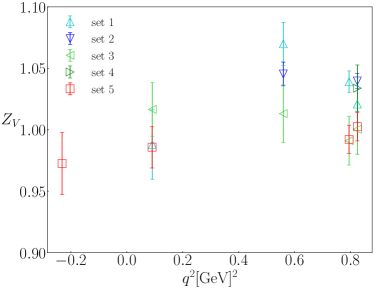
Figure 5: $Z_{V}$ for the $c\to s$ vector current evaluated at different $q^{2}$ from the calculation with an NRQCD spectator quark using Eq. (10).

Table 7: $Z_{V}$ obtained at zero-recoil using an NRQCD spectator $b$ quark .

set	$c\to s$	$c\to d$
1	1.021(15)	1.041(18)
2	1.0397(61)	1.021(17)
3	1.000(20)	1.004(22)
4	1.034(19)	0.983(20)
5	1.003(12)	0.958(20)

Table 8: $Z_{V}$ for $c\to s$ obtained at zero-recoil using a HISQ spectator quark with different values of the heavy quark mass $m_{h}$.

set/$am_{h}$	$0.274$	$0.450$	$0.6$	$0.663$	$0.8$
3				1.026(32)	1.029(36)
5		1.006(17)	1.003(19)		1.000(20)
6	0.997(14)	0.994(17)	0.995(19)		0.995(22)

Table 9: $Z_{V}$ for $c\to d$ obtained at zero-recoil using a HISQ spectator quark with different values of the heavy quark mass $m_{h}$.

set/$am_{h}$	$0.274$	$0.450$	$0.6$	$0.663$	$0.8$
3				1.016(47)	1.019(50)
5		1.009(23)	1.004(25)		1.000(27)
6	0.996(22)	0.993(25)	0.994(28)		0.995(32)

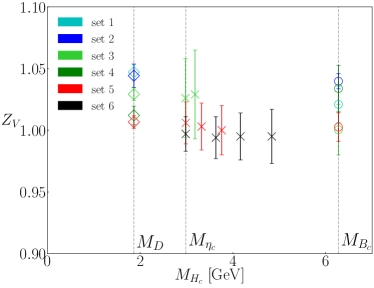
Figure 6: $Z_{V}$ of the $c\to s$ vector current from both the NRQCD and heavy-HISQ calculations are plotted alongside values from $D\to K$ Koponen et al. (2013). The NRQCD data is marked with circles, the heavy-HISQ data is marked with crosses, and finally the $D\to K$ values are given by diamonds. As expected, no significant dependence on the spectator mass is observed.

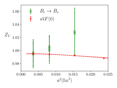
Figure 7: $Z_{V}$ from the $s\to s$ vector current from Chakraborty et al. (2017b) (red crosses) and the $c\to s$ vector current from the heavy-HISQ calculation given here (green squares). The curve is the fitted perturbative expansion, including discretisation effects, detailed in Chakraborty et al. (2017b). The red circle is an extrapolated value at the lattice spacing associated with the superfine lattice.

The $Z_{V}$ factor in Eq. (10) is associated only with the local vector current operator and should be independent of the spectator quark. $Z_{V}$ values obtained in the different calculations are tabulated in Tables 7, 8 and 9. Good agreement is seen on set 5 at zero-recoil between the results with NRQCD and heavy-HISQ spectator quarks. Dependence on the mass of the spectator quark is displayed in Fig. 6. The plot includes values from the analogous calculation for the $D\to K$ case Koponen et al. (2013). For $D\to K$, a charm quark decays into a strange quark, as in $B_{c}\to B_{s}$, but here the spectator quark is a light quark, much less massive than the heavy spectator quark in $B_{c}\to B_{s}$. The $Z_{V}$ from $B_{c}\to B_{s}$ and $D\to K$ in Fig. 6 are nevertheless in good agreement, demonstrating negligible dependence on the mass of the quark spectating the $c\to s$ transition.

It is also of interest to compare vector current renormalisation factors for different masses of quark featuring in the current. For example, Chakraborty et al. (2017b) calculates the local $\overline{s}\gamma_{\mu}s$ vector current renormalisation factor from an $\eta_{s}\to\eta_{s}$ 3-point correlation function at $q^{2}=0$ on the 2+1+1 MILC ensembles. This gave very precise values and it was possible to fit $Z_{V}$ to a perturbative expansion in $\alpha_{s}$ (including the known first-order term) along with discretisation effects. The fit is plotted in Fig. 7 alongside $Z_{V}$ for $c\to s$ values determined in this study. This plot shows differing behaviour as a function of $a^{2}$. The value for $Z_{V}$, determined non-perturbatively, is a combination of the underlying perturbative series in $\alpha_{s}$ evaluated at a scale related to the lattice spacing and discretisation effects that depend on how it was determined. Since the underlying perturbative series is common to different determinations, comparison will reveal the differing discretisation effects. Fig. 7 shows this in the comparison of our $Z_{V}$ values for the local $\overline{s}\gamma_{\mu}c$ current with those determined for the local $\overline{s}\gamma_{\mu}s$ current. In the limit of vanishing lattice spacing, where discretisation effects vanish, the renormalisation factors are in agreement.

One might worry that the large errors appearing in Fig. 7 for the $\overline{s}\gamma_{\mu}c$ renormalisation factors determined here would carry forward into our determination of the form factor $f_{+}$. However, the vector current matrix element at zero recoil, which contributes the dominant error in $Z_{V}$, is highly correlated with the vector matrix elements at non-zero recoil. These correlations cancel in the ratio $\mathcal{V}^{0}/\mathcal{V}^{0}(q^{2}_{\text{max}})$ appearing when using Eq. (10) to construct the renormalised current $Z_{V}\mathcal{V}^{0}$ appearing in Eqs. (12) and (13). Hence, the uncertainty in the renormalisation factor is not a large contribution to our final uncertainty in the form factors.

III.3 Form Factors

Fig. 8 provides an example of the extracted values for the form factor $f_{+}$, comparing results from the NRQCD and heavy-HISQ spectator calculations. The lines on the figures connect data on the same set at a given $am_{h}$ value and are present as a guide only. The spread of the heavy-HISQ data for different heavy quark masses is small, and the NRQCD and heavy-HISQ results are in good agreement on the fine lattice. Discretisation effects are more noticeable for the case of an NRQCD spectator quark, especially on the coarsest lattices, sets 1 and 2. We believe that they result from the $B_{c}$ meson in the calculation since the effects are comparable to those seen in the $B_{c}$ meson decay constant study with NRQCD $b$ quarks in Colquhoun et al. (2015). Data points outside the physical region of momentum transfer are unphysical but nevertheless aid the fit.

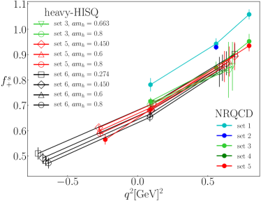
Figure 8: $f_{+}$ form factor data for $B_{c}^{+}\to B_{s}^{0}\overline{\ell}\nu_{\ell}$ from both the NRQCD and heavy-HISQ approaches. The NRQCD form factor data is given by filled circles; the heavy-HISQ data, by open circles. Data points on a given set and for a given heavy quark mass are joined by lines to guide eye.

IV Discussion

IV.1 $z$ Expansion

The four form factors, $f_{0}$ and $f_{+}$ for each of the $B_{c}\to B_{s}$ and $B_{c}\to B_{d}$ processes, at all momenta on all the lattices, are fit simultaneously to a functional form which allows for dependence on the lattice spacing $a$ and bare quark masses. The fit is carried out using the lsqfit package Lepage (qfit) that implements a least-squares fitting procedure. As is now standard, we map the semileptonic region $0<q^{2}<(M_{B_{c}}-M_{B_{s(d)}})^{2}$ to a region on the real axis within the unit circle through

$$z(q^{2}) =\frac{\sqrt{t_{+}-q^{2}}-\sqrt{t_{+}-t_{0}}}{\sqrt{t_{+}-q^{2}}+\sqrt{t_{+}-t_{0}}},$$ (16)

so that the form factors can be approximated by a truncated power series in $z$. Here we choose the parameter $t_{0}$ to be 0 so that the points $q^{2}=0$ and $z=0$ coincide. The parameter $t_{+}$ is in principle the threshold for production of mesons, the lightest being $D$ + $K$, from the $c\overline{s}$ current in the $t$-channel. It is convenient here, however, to work with $t_{+}=(M_{B_{c}}+M_{B_{s(d)}})^{2}$, but this gives a very small range for $z$ because then $t_{+}\gg t_{-}$. To correct for this we rescale $z$.

The rescaling factor that we use is $|z(M_{p}^{2})|^{-1}$, where $M_{p}$ is the mass of the nearest $c\overline{s}$ or $c\overline{d}$ meson pole (we use the same mass for both vector and scalar form factors for convenience). For $B_{c}\to B_{s}$ we take $M_{p}$ as the mass of the vector meson $D_{s}^{*}$ and for $B_{c}\to B_{d}$, the mass of $D^{*0}$. Thus, we define

$$z_{p}(q^{2}) =\frac{z(q^{2})}{|z(M_{p}^{2})|}.$$ (17)

$z_{p}$ then has a range more commensurate to that for the corresponding $D$ decay and the polynomial coefficients in $z_{p}$ are $\mathcal{O}(1)$. Coefficients of the conventional expansion in terms of $z$ can easily be obtained from the expansion in $z_{p}$. Using $z_{p}$ also avoids introducing large heavy mass dependence through the $z$ transform in the heavy-HISQ case, which otherwise would require large $\Lambda_{\text{QCD}}/M_{H_{c}}$ coefficients in the heavy-HISQ fit. Note that in the case of the heavy-HISQ spectator, the $B$-meson masses above in $t_{+}$ are replaced by the appropriate heavy meson masses at each value of $am_{h}$ (see Sec. IV.3).

IV.2 NRQCD Form Factor Fits

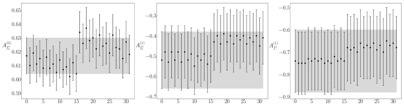
Figure 9: $z_{p}$ expansion coefficients, for the calculation with an NRQCD spectator quark, computed using the variations of correlator fit parameters listed in Table 5 for the $B_{c}\rightarrow B_{s}$ form factors. The integer $x$ coordinate of each result is given by $n_{\text{var}}^{(1)}+2n_{\text{var}}^{(2)}+4n_{\text{var}}^{(3)}+8n_{\text{var}}^{(4)}+16n_{\text{var}}^{(5)}$ where $n_{\text{var}}^{(i)}=0,1$ corresponding to the first and second fits respectively listed in Table 5 of set $i$.

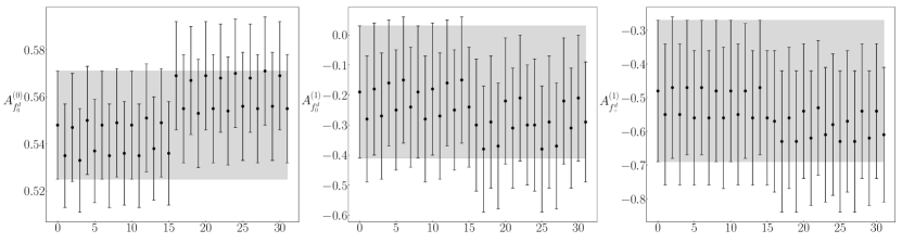
Figure 10: $z_{p}$ expansion coefficients, for the calculation with an NRQCD spectator quark, computed using the variations of correlator fit parameters listed in Table 5 for the $B_{c}\rightarrow B_{d}$ form factors. The $x$ coordinate is the same as that in Fig. 9.

The form factor results from the calculation with NRQCD spectator quark are fit to

$$f(q^{2})= \hskip 2.84526ptP(q^{2})\sum_{n=0}^{N}b^{(n)}z_{p}^{n}.$$ (18)

Here, the dominant pole structure is represented by a factor $P(q^{2})$ given by $(1-q^{2}/M^{2}_{\text{res}})^{-1}$ with $M_{\text{res}}$ the mass of the relevant $c\overline{s}$ or $c\overline{d}$ meson (the vector meson for $f_{+}$ and the scalar for $f_{0}$). We take the values of $M_{\text{res}}$ from current experiment Tanabashi et al. (2018): $M_{D_{s}^{*}}=2.112$ GeV, $M_{D_{s0}^{*}}=2.317$ GeV, $M_{D^{*}}=2.01027$ GeV, and $M_{D_{0}^{*}}=2.300$ GeV. We do not include uncertainties in these values since $P(q^{2})$ is a purely fixed factor designed to remove much of the $q^{2}$-dependence from the form factors. For our lattice results uncertainties enter $P(q^{2})$ from the uncertainty in our determination of $q^{2}$ in physical units, including that from the determination of the lattice spacing.

$P(q^{2})$ multiplies a polynomial in $z_{p}$, and the polynomial coefficients are

$$b^{(n)}= \hskip 2.84526ptA^{(n)}\Big{\{}1+B^{(n)}(am_{c}/\pi)^{2}+C^{(n)}(am_{c}/\pi)^{4}$$

$$+ \kappa_{1}^{(n)}\frac{\delta m_{l}^{\text{sea}}}{10m_{s}^{\text{tuned}}}+\kappa_{2}^{(n)}\frac{\delta m_{s}^{\text{sea}}}{10m_{s}^{\text{tuned}}}+\kappa_{3}^{(n)}\frac{\delta m_{c}^{\text{sea}}}{m_{c}^{\text{tuned}}}$$

$$+ \kappa^{(n)}_{4}\frac{\delta m_{s}^{\text{val}}}{10m_{s}^{\text{tuned}}}+\kappa^{(n)}_{5}\frac{\delta m_{c}^{\text{val}}}{m_{c}^{\text{tuned}}}+\kappa^{(n)}_{6}\frac{\delta m_{b}^{\text{val}}}{m_{b}^{\text{tuned}}}\Big{\}}.$$

The parameters $\kappa^{(n)}_{j}$ allow for errors associated with mistunings of both sea and valence quark masses. The term accounting for mistuning of valence strange quarks is included only for the $B_{c}\to B_{s}$ transition. The tuned masses $m_{s}^{\text{tuned}}$ and $m_{c}^{\text{tuned}}$ are the valence quark masses that yield physical $\eta_{s}$ and $\eta_{c}$ meson masses respectively in the sea of 2+1+1 flavours of sea quark. Values for $m_{s}^{\text{tuned}}$ and $m_{c}^{\text{tuned}}$ were obtained from Chakraborty et al. (2015). Also, $m_{l}^{\text{tuned}}$ is fixed by multiplying $m_{s}^{\text{tuned}}$ by the physical ratio

$$\frac{m_{l}}{m_{s}}= \hskip 2.84526pt\frac{1}{27.18(10)}$$ (20)

obtained from Bazavov et al. (2018). For the $b$ quark, we take tuned values of the quark mass from Table XII in Dowdall et al. (2012).

For each of the sea and valence quark flavours, $\delta m^{\text{sea}}$ and $\delta m^{\text{val}}$ are given by

$$\delta m^{\text{sea}}= \hskip 2.84526ptm^{\text{sea}}-m^{\text{tuned}}$$

$$\delta m^{\text{val}}= \hskip 2.84526ptm^{\text{val}}-m^{\text{tuned}},$$ (21)

giving estimates of the extent that the quark masses deviate from the ideal choices in which appropriate meson masses are exactly reproduced.

For prior values on the parameters in Eq. (IV.2), we use $0(1)$ for $A^{(n)}$, $B^{(n)}$ and $C^{(n)}$, and $0.0(5)$ for $\kappa_{(j)}$. The power series in Eq. (18) is truncated to include up to the $z_{p}^{3}$ term. Fits without a pole, i.e. $P(q^{2})=1$, yield no statistically significant discrepancies. This is not surprising since the poles are far away from the physical region of $q^{2}$, and so the pole effect on the form factor can be reasonably absorbed into the polynomial. Finally, the kinematic relation

$$f_{0}(0)=f_{+}(0)$$ (22)

is imposed on the fit as a constraint (we have tested that removing this constraint makes very little difference to the fit in fact and $f_{+}(0)-f_{0}(0)$ is zero to well within 1$\sigma$.).

Constraints on $b^{(n)}$ from unitarity, as in the Bourrely-Caprini-Lellouch (BCL) Bourrely et al. (2009) and Boyd-Grinstein-Lebed (BGL) Boyd et al. (1996) expansions, are unnecessary here since the full range of physical momentum transfer can be reached and so extrapolation in $q^{2}$, which may benefit in accuracy from imposing these constraints, is not required. Hence, more complicated fit forms that impose additional physical constraints are not expected to be appreciably advantageous.

In Figs. 9 and 10, we demonstrate that the form factors in the physical-continuum limit are insensitive to the choice of the parameters in the fits of the correlators. As can be seen in the figures, the coefficients in the fits of the form factors are stable, within their uncertainties, as the correlator fits on different sets are varied.

The fitted form factors from the NRQCD spectator case exhibit errors no greater than $4\%$ across the entire physical range of $q^{2}$ when tuned to the physical-continuum limit. Figs. 11, 12, 13 and 14 show the results on all the lattices along with the fitted function for the form factors in the physical-continuum limit.

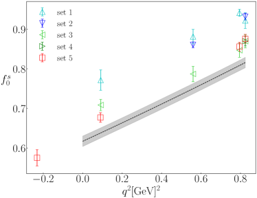
Figure 11: Lattice results and fitted $f_{0}$ form factor data for $B_{c}^{+}\to B_{s}^{0}\overline{\ell}\nu_{\ell}$ with an NRQCD $b$ quark. The grey band shows the fitted form factor tuned to the limit of vanishing lattice spacing and physical quark masses.

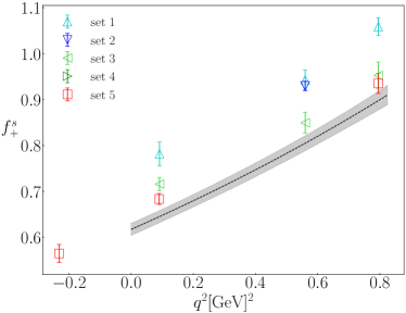
Figure 12: Lattice results and fitted $f_{+}$ form factor data for $B_{c}^{+}\to B_{s}^{0}\overline{\ell}\nu_{\ell}$ with an NRQCD $b$ quark. The grey band shows the fitted form factor tuned to the limit of vanishing lattice spacing and physical quark masses.

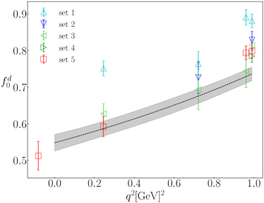
Figure 13: Lattice results and fitted $f_{0}$ form factor data for $B_{c}^{+}\to B^{0}\overline{\ell}\nu_{\ell}$ with an NRQCD $b$ quark. The grey band shows the fitted form factor tuned to the limit of vanishing lattice spacing and physical quark masses.

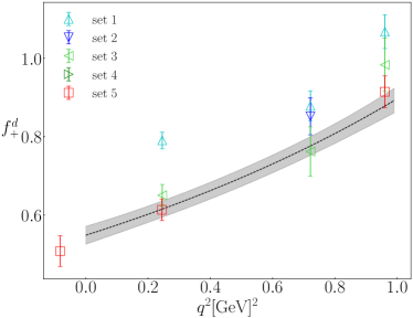
Figure 14: Fitted $f_{+}$ form factor data for $B_{c}^{+}\to B^{0}\overline{\ell}\nu_{\ell}$ with an NRQCD $b$ quark. The grey band shows the fitted form factor tuned to the limit of vanishing lattice spacing and physical quark masses.

Table 10: A selection of $f_{0}$ and $f_{+}$ fit parameters from our fit to Eq. (IV.2) with an NRQCD-$b$ quark, demonstrating the leading order momentum and lattice spacing dependence. Note that the discretisation effects in the $f_{0}$ and $f_{+}$ fits are allowed to vary independently of each other with separate $B^{(0)}$ parameters. In practice, as the Table shows, the fit returns very similar values.

	$f_{0}^{s}$	$f_{0}^{d}$	$f_{+}^{s}$	$f_{+}^{d}$
$A^{(0)}$	0.617(13)	0.548(23)	0.617(13)	0.548(23)
$A^{(1)}$	-0.52(14)	-0.19(22)	-0.74(14)	-0.48(21)
$A^{(2)}$	-0.63(63)	0.05(74)	-0.29(72)	0.12(77)
$B^{(0)}$	1.44(38)	1.45(46)	1.44(38)	1.45(46)

The $z_{p}^{0}$ and $z_{p}^{1}$ behaviour of the form factors is well resolved by our fit to Eq. (IV.2), as well as the $(am_{c}/\pi)^{2}z_{p}^{0}$ discretisation effect. Table 10 summarises the corresponding parameters from the fit. After fitting, other parameters show errors comparable to the width of their prior and are consistent with 0. In particular, quark mass mistuning coefficients simply return their prior value.

IV.3 Heavy-HISQ Form Factor Fits

We take a similar approach to fitting the form factor results for the case of a heavy-HISQ spectator. Now we have results at multiple heavy-quark masses and the conversion from $q^{2}$ to $z$-space (Eq. (16)) uses the values of $M_{H_{c}}$ and $M_{H_{s}}$ or $M_{H_{d}}$, as appropriate, from our calculation. We then rescale $z$ at each $m_{h}$ as described in Sec. IV.1 (Eq. (17)). This rescaling gives a similar $z$-range for each $m_{h}$ and avoids introducing spurious dependence on $m_{h}$ that comes simply from the $z$-transform. I The heavy-HISQ results are then fit to a form that is a product of $P(q^{2})$ and a polynomial in $z_{p}$ as for the NRQCD case. We now require a fit form for the polynomial coefficients that accounts for $(am_{h})^{2n}$ discretisation effects as well as physical dependence on $m_{h}$, however. Motivated by heavy quark effective theory (HQET) we express this physical heavy mass dependence as a power series in $\Lambda_{\text{QCD}}/M_{H_{c}}$. The form factor data from the heavy-HISQ approach is fit to

$$f(q^{2})=P(q^{2}) \sum_{n,i,j,k=0}^{3}A^{(n)}_{ijk}z_{p}^{n}$$

$$\times\left(\frac{am_{c}}{\pi}\right)^{2i}\left(\frac{am_{h}}{\pi}\right)^{2j}\Delta_{H_{c}}^{(k)}\mathcal{N}_{\text{mis}}^{(n)},$$ (23)

where, for $k=0$, $\Delta_{M}^{(k)}=1$ and, for $k\neq 0$,

$$\Delta_{H_{c}}^{(k)}=\left(\frac{\Lambda_{\text{QCD}}}{M_{H_{c}}}\right)^{k}-\left(\frac{\Lambda_{\text{QCD}}}{M_{B_{c}}}\right)^{k}$$ (24)

where we take $\Lambda_{QCD}=500\text{MeV}$. The mistuning terms are given by

$$\mathcal{N}_{\text{mis}}^{(n)} =1+\frac{\delta m_{c}^{\text{val}}}{m_{c}^{\text{tuned}}}a_{n}+\frac{\delta m_{c}^{\text{sea}}}{m_{c}^{\text{tuned}}}b_{n}$$

$$+\frac{\delta m_{s}^{\text{val}}}{10m_{s}^{\text{tuned}}} c_{n}+\frac{\delta m_{s}^{\text{sea}}}{10m_{s}^{\text{tuned}}}d_{n}+\frac{\delta{m_{l}}}{10m_{s}^{\text{tuned}}}e_{n},$$ (25)

where we only include the term proportional to $\delta m_{s}^{\text{val}}$ for the $B_{c}\rightarrow B_{s}$ case. $P(q^{2})$, $\delta{m}$ and the tuned masses have the same definitions as in the NRQCD case (Sec. IV.2). In the physical continuum limit, this form collapses to $P(q^{2})\sum_{n}z_{p}^{n}A^{(n)}_{000}$. Again we apply the constraint $f_{0}(0)=f_{+}(0)$ in the continuum limit (by fixing $A_{000}^{(0)}$ to be the same in the two cases).

Results for the extrapolated form factors are given in Figs. 15, 16, 17 and 18 together with the corresponding lattice data. For the $B_{c}\rightarrow B_{s}$ case $a_{n}$ and $c_{n}$ take prior values $0(1)$ and $b_{n}$, $d_{n}$ and $e_{n}$ take prior values $0(0.3)$ to reflect the fact that they enter through loop effects. In the $B_{c}\rightarrow B_{d}$ case we take prior values of $0(1)$ for $a_{n}$ and $e_{n}$ and $0(0.3)$ for $b_{n}$ and $d_{n}$. In both cases we take prior values of $0(1)$ for $A_{ijk}^{n}$ except for when $i=1$ or $j=1$ where we use a prior values of $0(0.3)$ to account for the HISQ one loop improvement.

As in the case of an NRQCD spectator quark, we present coefficients of the form factors fits from many different fits of the correlator data. Figs. 19 and 20, show that the coefficients are insensitive to the choice of the parameters in the fits of the correlators.

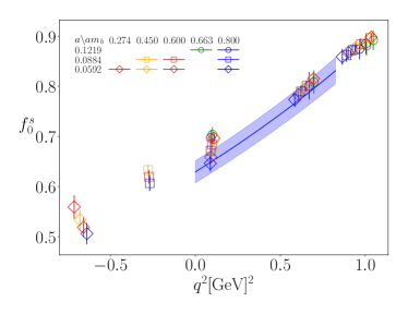
Figure 15: Heavy-HISQ form factor results for $f^{s}_{0}$ together with the fitted curve at the physical point with its error band.

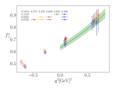
Figure 16: Heavy-HISQ form factor results for $f_{+}^{s}$ together with the fitted curve at the physical point with its error band.

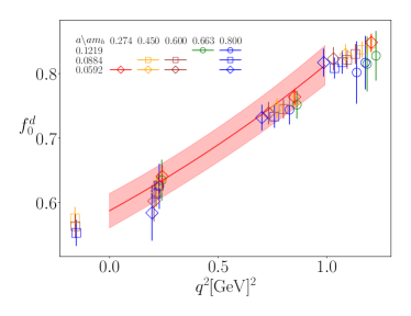
Figure 17: Heavy-HISQ form factor results for $f^{d}_{0}$ together with the fitted curve at the physical point with its error band.

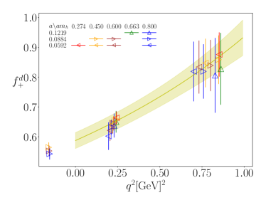
Figure 18: Heavy-HISQ form factor results for $f_{+}^{d}$ together with the fitted curve at the physical point with its error band.

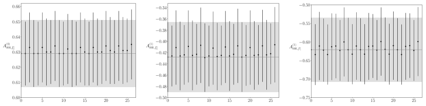
Figure 19: $z_{p}$ expansion coefficients, for the calculation with a HISQ spectator quark, computed using the variations of correlator fit parameters listed in Table 6 for the $B_{c}\rightarrow B_{s}$ form factors. The integer $x$ coordinate of each result is given by $n_{\text{var}}^{(3)}+3n_{\text{var}}^{(5)}+9n_{\text{var}}^{(6)}$ where $n_{\text{var}}^{(i)}=0,1,2$ corresponding to original, first and second variations respectively listed in Table 6 of set $i$.

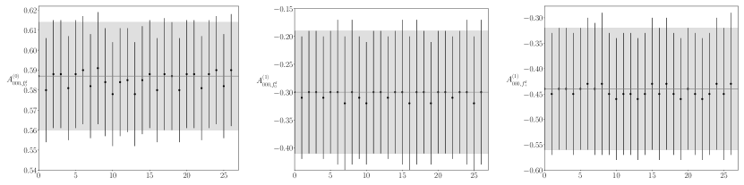
Figure 20: $z_{p}$ expansion coefficients, for the calculation with a HISQ spectator quark, computed using the variations of correlator fit parameters listed in Table 6 for the $B_{c}\rightarrow B_{d}$ form factors. The $x$ coordinate is the same as that in Fig. 19.

IV.4 Chained Fit

The form factor functions tuned to the physical-continuum limit from NRQCD and heavy-HISQ are compared in Figs. 21, 22, 23 and 24 in $z$-space. There is good agreement across the entire physical range of $z$, with particularly good agreement for the more accurate $B_{c}\rightarrow B_{s}$ case.

Whilst the fit forms for the form factors from NRQCD and heavy-HISQ at Eqs. (18) and (23) differ in appearance, they both allow for effects of discretisation and mistuning of the quark masses. In the continuum limit with physical masses, the two forms collapse such that the parameters $A^{(n)}$ from Eq. (IV.2) and $A_{000}^{(n)}$ from Eq. (23) coincide. Plotted among the functions from the heavy-HISQ and NRQCD calculations is a function arising from a ‘chained’ fit where the $A_{000}^{(n)}$ from the heavy-HISQ fit were used as prior distributions for the $A^{(n)}$ in the form factor fit forms in the NRQCD study. We label this fit NRQCD from heavy-HISQ in Figs. 21, 22, 23 and 24. As with the separate fits for each case of spectator quark, the form factors for $B_{c}\to B_{s}$ and $B_{c}\to B_{d}$ are fit simultaneously. This chained fit has $\chi^{2}/\text{d.o.f.}=1.1$ and is consistent with both the separate fits. We make our final predictions for the decay rates and values for $\Gamma|V|^{2}$ using the chained fit.

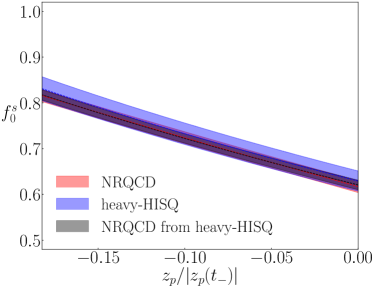
Figure 21: Fits of $f_{0}$ for $B_{c}^{+}\to B_{s}^{0}\overline{\ell}\nu_{\ell}$ tuned to the physical-continuum limit. The form factor is plotted against $z_{p}/|z_{p}(t_{-})|$.

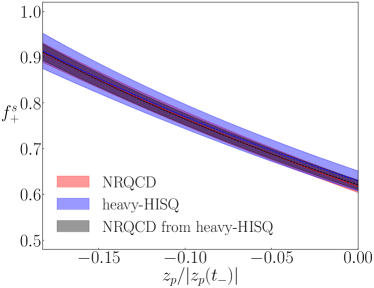
Figure 22: Fits of $f_{+}$ for $B_{c}^{+}\to B_{s}^{0}\overline{\ell}\nu_{\ell}$ tuned to the physical-continuum limit.

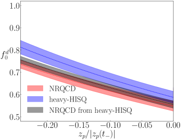
Figure 23: Fits of $f_{0}$ for $B_{c}^{+}\to B^{0}\overline{\ell}\nu_{\ell}$ tuned to the physical-continuum limit.

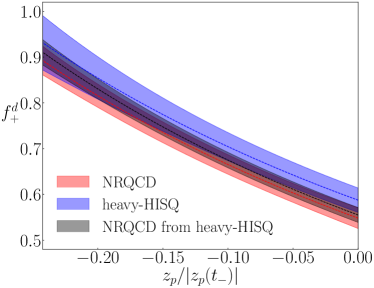
Figure 24: Fits of $f_{+}$ for $B_{c}^{+}\to B^{0}\overline{\ell}\nu_{\ell}$ tuned to the physical-continuum limit.

We include the coefficients $A_{0,+}^{(n)}$ from the chained fit in the ancillary json file BcBsd_ff_updated.json. To assist those who wish to import the form factors from these coefficients, we provide values that the form factors should take for both $q^{2}=0$ and $q^{2}_{\mathrm{max}}$ in Table 11.

Table 11: The form factors from the chained fit evaluated at $q^{2}=0$ and $q^{2}_{\mathrm{max}}$.

$q^{2}\;[\mathrm{GeV}]^{2}$	$f_{0}^{s}$	$f_{+}^{s}$	$f_{0}^{d}$	$f_{+}^{d}$
$0$	$0.621(10)$	$0.621(10)$	$0.555(16)$	$0.555(16)$
$q^{2}_{\mathrm{max}}$	$0.817(11)$	$0.911(18)$	$0.756(16)$	$0.910(28)$

IV.5 Dependence of the form factors on the spectator quark mass

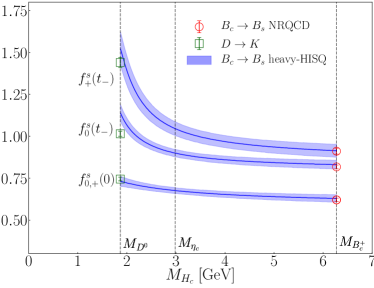
Figure 25: Values for the physical-continuum form factors $f_{0}^{s}=f_{+}^{s}$ at $q^{2}=0$ and $f_{0}^{s}$ and $f_{+}^{s}$ at $q^{2}_{\text{max}}$ are plotted against the mass of the heavy-charm pseudoscalar meson. The curve is the continuum limit of the heavy-HISQ fit function (Eq. (23)) extrapolated to the physical $B_{c}$ and $D$ masses. Note that the region in which the heavy-HISQ calculation has results is the region above $M_{\eta_{c}}$. See the text for a description of how the extrapolation down to the $D$ was done. Also plotted are the form factor results for $D\to K$ Koponen et al. (2013) (green squares) as well as the NRQCD $B_{c}\rightarrow B_{s}$ result presented in this work (red circles).

In order to build up a picture of the behaviour of form factors it is interesting to ask: how do the form factors for $c$ to $s/d$ decay depend on the mass of the spectator quark? We can answer that question with our heavy-HISQ calculation because we have results at a range of spectator quark masses from $m_{c}$ upwards (see Fig. 2). Our form factor fits (Sec. IV.3) enable us to extrapolate up to $m_{b}$. Our most accurate results are for the $c$ to $s$ decay case and we concentrate on that here.

Fig. 25 shows the fit curve from the heavy-HISQ results for $f^{s}_{+}$ and $f_{0}^{s}$ as a function of the heavy-charm meson mass (as a proxy for the spectator quark mass). The form factor curves that are plotted are those for $q^{2}=0$ (where $f_{+}=f_{0}$) and for the zero-recoil point ($q^{2}_{\text{max}}$). At $q^{2}_{max}$ the daughter meson is at rest in the rest-frame of the $H_{c}$ meson. The $q^{2}$ value at $q^{2}_{\text{max}}$ falls slowly as the heavy-quark mass increases above $m_{c}$ because the mass difference between $H_{c}$ and $H_{s}$ mesons falls. Examining the region between $M_{\eta_{c}}$ and $M_{B_{c}}$ in Fig. 25 we see almost no dependence on the spectator mass. The form factor value that shows the most dependence is $f_{+}(q^{2}_{max})$. This is not surprising because $f_{+}$ shows the biggest slope in $q^{2}$ close to $q^{2}_{\text{max}}$ and hence sensitivity to the value of $q^{2}_{\text{max}}$. Note that the curve from the heavy-HISQ analysis agrees with the NRQCD results at a spectator mass equal to that of the $b$. As discussed in the previous subsection, the form factors obtained from the two calculations agree across the full $q^{2}$ range.

We can also investigate the behaviour of the heavy-HISQ fit function as $m_{h}$ is taken below $m_{c}$ to $m_{l}$ where contact is made with results for $D\to K$ from Koponen et al. (2013). For the form factors at $q^{2}=0$, we have $P(q^{2})=1$ and our fit form at Eq. (23) depends only on $M_{H_{c}}$. This permits a straightforward extrapolation to the point $M_{H_{c}}=M_{D}$ in the continuum limit. For the form factors at zero-recoil ($q^{2}_{\text{max}}$), constructing the extrapolation curve is complicated by requiring the dependence of $q^{2}_{\text{max}}$ on the mass of the spectator quark. This requires knowledge of $M_{H_{s}}$ as a function of $M_{H_{c}}$. To achieve this, we fit our values of $M_{H_{s}}$ taken from set 6, together with physical values from experiment Tanabashi et al. (2018) at $m_{h}=m_{l},m_{b}$ (i.e. $M_{K}$ and $M_{B_{s}}$), using a simple fit form $M_{H_{s}}=M_{H_{c}}(1+\sum_{n=1}^{4}\omega_{n}(\Lambda_{QCD}/M_{H_{c}})^{n}+A(a\Lambda_{QCD})^{2}+B(a\Lambda_{QCD})^{4})$. Here $A$, $B$ and $\omega_{n}$ take prior values $0(2)$ and we do not include $a\Lambda$ terms for data from Tanabashi et al. (2018). We find this fit function reproduces our data, as well as the physical values, well. Fig. 25 also shows the result of this downward extrapolation. Whilst this extrapolation below $m_{c}$ is outside the region where HQET is expected to be valid, the curves nevertheless show approximately the correct amount of upward movement necessary to reproduce the $D\rightarrow K$ results in Koponen et al. (2013) for $f_{+}$ and $f_{0}$ at zero-recoil and $q^{2}=0$. The form factors at $q^{2}=0$ continue to show almost no spectator mass dependence, and this is in agreement with the $D\rightarrow K$ results.

IV.6 Decay rate

The hadronic quantity required for determining the decay rate and branching fraction is the integral

$$\Gamma|V|^{-2}=\frac{G_{F}^{2}}{24\pi^{3}}\int_{0}^{t_{-}}dq^{2}\hskip 2.84526pt|\mathbf{p}_{2}|^{3}|f_{+}(q^{2})|^{2},$$ (26)

where $V$ is the CKM element $V_{cs}$ or $V_{cd}$. Table 12 gives values for this quantity for each of the $B_{c}\to B_{s}$ and $B_{c}\to B_{d}$ processes based on the NRQCD and heavy-HISQ chained form factor fit described in Sec. IV.4.

Table 12: Final results of the weighted integral of $|f_{+}(q^{2})|^{2}$ over the physical range of squared 4-momentum transfer. Units are MeV.

	$B_{c}^{+}\to B_{s}^{0}\overline{\ell}\nu_{\ell}$	$B_{c}^{+}\to B^{0}\overline{\ell}\nu_{\ell}$
$\Gamma|V|^{-2}$	$1.738(55)\times 10^{-11}$	$2.29(12)\times 10^{-11}$

Values for different $q^{2}$ bins can also be obtained. Proceeding with the total decay rate, combining these results with existing CKM matrix values Tanabashi et al. (2018) $V_{cs}=0.997(17)$ and $V_{cd}=0.218(4)$ yields the predictions

$$\Gamma(B_{c}^{+}\to B_{s}^{0}\overline{\ell}\nu_{\ell}) =26.25(90)(83)\times 10^{9}\hskip 2.84526pt\text{s}^{-1}$$

$$\Gamma(B_{c}^{+}\to B^{0}\overline{\ell}\nu_{\ell}) =1.650(61)(84)\times 10^{9}\hskip 2.84526pt\text{s}^{-1}$$ (27)

where the CKM matrix elements are responsible for the first errors and the second errors arise from our lattice calculations. The dominant source of lattice QCD uncertainty is the fitting of 2-point and 3-point correlators described in Sec. II.2.3.

We can convert these results for the decay width into a branching fraction using the lifetime of the $B_{c}$ meson, $513.49(12.4)\;\mathrm{fs}$ Aaij et al. (2015). This gives

$$\mathcal{B}(B_{c}^{+}\to B_{s}^{0}\overline{\ell}\nu_{\ell}) =0.01348(46)(33)(43)$$

$$\mathcal{B}(B_{c}^{+}\to B^{0}\overline{\ell}\nu_{\ell}) =0.000847(31)(43)(20)$$ (28)

where now the third uncertainty is from the lifetime.

We also present the ratio of the $\Gamma|V|^{-2}$ for $B_{c}\rightarrow B_{s}$ to $B_{c}\rightarrow B_{d}$ taking correlations into account between the numerator and denominator. From the chained fit of $B_{c}^{+}\to B_{s}^{0}\overline{\ell}\nu_{\ell}$ and $B_{c}^{+}\to B^{0}\overline{\ell}\nu_{\ell}$ form factors, we obtain

$$\frac{\Gamma(B_{c}^{+}\to B_{s}^{0}\overline{\ell}\nu_{\ell})|V_{cd}|^{2}}{\Gamma(B_{c}^{+}\to B^{0}\overline{\ell}\nu_{\ell})|V_{cs}|^{2}}=0.759(44).$$ (29)

In fact the uncertainty is roughly the same as if we were to treat the numerator and denominator as uncorrelated.

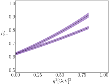
Figure 26: Final form factors from the chained fits of $f_{0}$ (below) and $f_{+}$ (above) for $B_{c}^{+}\to B_{s}^{0}\overline{\ell}\nu_{\ell}$ in the physical-continuum limit, plotted against the entire range of physical $q^{2}$. This fit is described in Sec. IV.4.

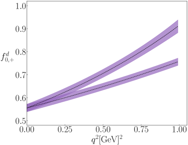
Figure 27: Final form factors from the chained fits of $f_{0}$ (below) and $f_{+}$ (above) for $B_{c}^{+}\to B^{0}\overline{\ell}\nu_{\ell}$ in the physical-continuum limit, plotted against the entire range of physical $q^{2}$. This fit is described in Sec. IV.4.

V Conclusions

We have reported here the first calculations of the decay rates $\Gamma(B_{c}^{+}\to B_{s}^{0}\overline{\ell}\nu_{\ell})$ and $\Gamma(B_{c}^{+}\to B^{0}\overline{\ell}\nu_{\ell})$, demonstrating the success of lattice QCD in studying decays of heavy-light mesons. The use of HISQ-HISQ $c\to s(d)$ currents allows for a non-perturbative renormalisation using the PCVC. We used two different formulations for the spectator $b$ quark, heavy-HISQ and NRQCD. Results from the heavy-HISQ calculations are in good agreement with the physical-continuum form factors derived from the calculations using NRQCD $b$ quarks, giving us confidence in assessing and controlling the systematic errors in each formulation. Simulating at a variety of spectator masses in the heavy-HISQ calculation has provided a check of the spectator-independence of the renormalisation procedure for the vector current. The NRQCD study also accessed $Z_{V}$ away from zero-recoil to scrutinise momentum independence.

Our final form factors from the chained fit that combines both NRQCD and heavy-HISQ results are plotted against $q^{2}$ in Figs. 26 and 27.

The decay rates are predicted from our calculation with 4.6% and 6.3% uncertainty for $\Gamma(B_{c}^{+}\to B_{s}^{0}\overline{\ell}\nu_{\ell})=26.2(1.2)\times 10^{9}\hskip 2.84526pt\text{s}^{-1}$ and $\Gamma(B_{c}^{+}\to B^{0}\overline{\ell}\nu_{\ell})=1.65(10)\times 10^{9}\hskip 2.84526pt\text{s}^{-1}$ respectively. There is scope for significant improvement should future experiment demand more precision from the lattice. Such improvement would be readily achieved by the inclusion of lattices with a finer lattice in the heavy-HISQ calculation. ‘Ultrafine’ lattices with $a\approx 0.045$ [fm] were used in McLean et al. (2019) to provide results nearer to the physical-continuum limit with $am_{h}\approx am_{b}$. Larger statistical samples could also be obtained on the lattices used here, at the cost of more computational resources.

References

- Aubin et al. (2005) C. Aubin et al. (Fermilab Lattice, MILC, HPQCD), Phys. Rev. Lett. 94, 011601 (2005), arXiv:hep-ph/0408306 [hep-ph] .
- Na et al. (2010) H. Na, C. T. H. Davies, E. Follana, G. P. Lepage, and J. Shigemitsu (HPQCD), Phys. Rev. D82, 114506 (2010), arXiv:1008.4562 [hep-lat] .
- Koponen et al. (2013) J. Koponen, C. T. H. Davies, G. C. Donald, E. Follana, G. P. Lepage, H. Na, and J. Shigemitsu, (2013), arXiv:1305.1462 [hep-lat] .
- Donald et al. (2014) G. C. Donald, C. T. H. Davies, J. Koponen, and G. P. Lepage (HPQCD), Phys. Rev. D90, 074506 (2014), arXiv:1311.6669 [hep-lat] .
- Bazavov et al. (2014) A. Bazavov et al. (Fermilab Lattice, MILC), Phys. Rev. D90, 074509 (2014), arXiv:1407.3772 [hep-lat] .
- Lubicz et al. (2017) V. Lubicz, L. Riggio, G. Salerno, S. Simula, and C. Tarantino (ETM), Phys. Rev. D96, 054514 (2017), [erratum: Phys. Rev.D99,no.9,099902(2019)], arXiv:1706.03017 [hep-lat] .
- Lepage et al. (1992) G. P. Lepage, L. Magnea, C. Nakhleh, U. Magnea, and K. Hornbostel, Phys. Rev. D46, 4052 (1992), arXiv:hep-lat/9205007 [hep-lat] .
- Dowdall et al. (2012) R. J. Dowdall et al. (HPQCD), Phys. Rev. D85, 054509 (2012), arXiv:1110.6887 [hep-lat] .
- McNeile et al. (2010) C. McNeile, C. T. H. Davies, E. Follana, K. Hornbostel, and G. P. Lepage, Phys. Rev. D82, 034512 (2010), arXiv:1004.4285 [hep-lat] .
- McNeile et al. (2012) C. McNeile, C. T. H. Davies, E. Follana, K. Hornbostel, and G. P. Lepage (HPQCD), Phys. Rev. D85, 031503 (2012), arXiv:1110.4510 [hep-lat] .
- McLean et al. (2019) E. McLean, C. T. H. Davies, J. Koponen, and A. T. Lytle, (2019), arXiv:1906.00701 [hep-lat] .
- Follana et al. (2007) E. Follana, Q. Mason, C. Davies, K. Hornbostel, G. P. Lepage, J. Shigemitsu, H. Trottier, and K. Wong (HPQCD, UKQCD), Phys. Rev. D75, 054502 (2007), arXiv:hep-lat/0610092 [hep-lat] .
- Borsanyi et al. (2012) S. Borsanyi et al., JHEP 09, 010 (2012), arXiv:1203.4469 [hep-lat] .
- Chakraborty et al. (2017a) B. Chakraborty, C. T. H. Davies, P. G. de Oliviera, J. Koponen, G. P. Lepage, and R. S. Van de Water, Phys. Rev. D96, 034516 (2017a), arXiv:1601.03071 [hep-lat] .
- Chakraborty et al. (2015) B. Chakraborty, C. T. H. Davies, B. Galloway, P. Knecht, J. Koponen, G. C. Donald, R. J. Dowdall, G. P. Lepage, and C. McNeile, Phys. Rev. D91, 054508 (2015), arXiv:1408.4169 [hep-lat] .
- Dowdall et al. (2013) R. J. Dowdall, C. T. H. Davies, G. P. Lepage, and C. McNeile, Phys. Rev. D88, 074504 (2013), arXiv:1303.1670 [hep-lat] .
- Bazavov et al. (2010) A. Bazavov et al. (MILC), Phys. Rev. D82, 074501 (2010), arXiv:1004.0342 [hep-lat] .
- Bazavov et al. (2013) A. Bazavov et al. (MILC), Phys. Rev. D87, 054505 (2013), arXiv:1212.4768 [hep-lat] .
- Bazavov et al. (2016) A. Bazavov et al. (MILC), Phys. Rev. D93, 094510 (2016), arXiv:1503.02769 [hep-lat] .
- Hart et al. (2009) A. Hart, G. M. von Hippel, and R. R. Horgan (HPQCD), Phys. Rev. D79, 074008 (2009), arXiv:0812.0503 [hep-lat] .
- Koponen et al. (2017) J. Koponen, A. C. Zimermmane-Santos, C. T. H. Davies, G. P. Lepage, and A. T. Lytle, Phys. Rev. D96, 054501 (2017), arXiv:1701.04250 [hep-lat] .
- Koponen (2016) J. Koponen (HPQCD), Proceedings, 33rd International Symposium on Lattice Field Theory (Lattice 2015): Kobe, Japan, July 14-18, 2015, PoS LATTICE2015, 119 (2016).
- (23) MILC Code Repository, https://github.com/milc-qcd.
- Sachrajda and Villadoro (2005) C. T. Sachrajda and G. Villadoro, Phys. Lett. B609, 73 (2005), arXiv:hep-lat/0411033 [hep-lat] .
- Guadagnoli et al. (2006) D. Guadagnoli, F. Mescia, and S. Simula, Phys. Rev. D73, 114504 (2006), arXiv:hep-lat/0512020 [hep-lat] .
- Aubin et al. (2004) C. Aubin, C. Bernard, C. E. DeTar, J. Osborn, S. Gottlieb, E. B. Gregory, D. Toussaint, U. M. Heller, J. E. Hetrick, and R. Sugar (MILC), Phys. Rev. D70, 114501 (2004), arXiv:hep-lat/0407028 [hep-lat] .
- Gregory et al. (2011) E. B. Gregory et al. (HPQCD), Phys. Rev. D83, 014506 (2011), arXiv:1010.3848 [hep-lat] .
- Donald et al. (2012) G. C. Donald, C. T. H. Davies, R. J. Dowdall, E. Follana, K. Hornbostel, J. Koponen, G. P. Lepage, and C. McNeile, Phys. Rev. D86, 094501 (2012), arXiv:1208.2855 [hep-lat] .
- Lepage et al. (2002) G. P. Lepage, B. Clark, C. T. H. Davies, K. Hornbostel, P. B. Mackenzie, C. Morningstar, and H. Trottier, Lattice field theory. Proceedings, 19th International Symposium, Lattice 2001, Berlin, Germany, August 19-24, 2001, Nucl. Phys. Proc. Suppl. 106, 12 (2002), arXiv:hep-lat/0110175 [hep-lat] .
- Hornbostel et al. (2012) K. Hornbostel, G. P. Lepage, C. T. H. Davies, R. J. Dowdall, H. Na, and J. Shigemitsu (HPQCD), Phys. Rev. D85, 031504 (2012), arXiv:1111.1363 [hep-lat] .
- Bouchard et al. (2014) C. M. Bouchard, G. P. Lepage, C. Monahan, H. Na, and J. Shigemitsu (HPQCD), Phys. Rev. D90, 054506 (2014), arXiv:1406.2279 [hep-lat] .
- Chakraborty et al. (2018) B. Chakraborty, C. Davies, J. Koponen, and G. P. Lepage (HPQCD), Proceedings, 35th International Symposium on Lattice Field Theory (Lattice 2017): Granada, Spain, June 18-24, 2017, EPJ Web Conf. 175, 13027 (2018), arXiv:1710.07334 [hep-lat] .
- Tanabashi et al. (2018) M. Tanabashi et al. (Particle Data Group), Phys. Rev. D 98, 030001 (2018).
- Michael (1994) C. Michael, Phys. Rev. D49, 2616 (1994), arXiv:hep-lat/9310026 [hep-lat] .
- Dowdall et al. (2019) R. J. Dowdall, C. T. H. Davies, R. R. Horgan, G. P. Lepage, C. J. Monahan, J. Shigemitsu, and M. Wingate (HPQCD), Phys. Rev. D100, 094508 (2019), arXiv:1907.01025 [hep-lat] .
- Chakraborty et al. (2017b) B. Chakraborty, C. T. H. Davies, G. C. Donald, J. Koponen, and G. P. Lepage (HPQCD), Phys. Rev. D96, 074502 (2017b), arXiv:1703.05552 [hep-lat] .
- Colquhoun et al. (2015) B. Colquhoun, C. T. H. Davies, R. J. Dowdall, J. Kettle, J. Koponen, G. P. Lepage, and A. T. Lytle (HPQCD), Phys. Rev. D91, 114509 (2015), arXiv:1503.05762 [hep-lat] .
- Lepage (qfit) G. P. Lepage, lsqfit Version 11.1 (github.com/gplepage/lsqfit).
- Bazavov et al. (2018) A. Bazavov et al., Phys. Rev. D98, 074512 (2018), arXiv:1712.09262 [hep-lat] .
- Bourrely et al. (2009) C. Bourrely, I. Caprini, and L. Lellouch, Phys. Rev. D79, 013008 (2009), [Erratum: Phys. Rev.D82,099902(2010)], arXiv:0807.2722 [hep-ph] .
- Boyd et al. (1996) C. G. Boyd, B. Grinstein, and R. F. Lebed, Nucl. Phys. B461, 493 (1996), arXiv:hep-ph/9508211 [hep-ph] .
- Aaij et al. (2015) R. Aaij et al. (LHCb), Phys. Lett. B742, 29 (2015), arXiv:1411.6899 [hep-ex] .