The Full Color Two-Loop Six-Gluon All-Plus Helicity Amplitude

Abstract

We present the full color two-loop six-point all-plus Yang-Mills amplitude in compact analytic form. The computation uses four dimensional unitarity and augmented recursion.

I Introduction

Computing perturbative scattering amplitudes in gauge theories is a key tool in confronting theories of particle physics with experimental results and there is considerable demand for new predictions particularly at “Next-Next-Leading Order” (NNLO) Bendavid:2018nar ; Azzi:2019yne . Amplitudes are also the custodians of the symmetries of the theory and as such are important for exploring properties of theories which are not always manifest in a Lagrangian approach. Computing amplitudes in closed analytic form is particularly useful in this regard.

Amplitudes for the scattering of gluons within a gauge theory are key, being both important phenomenologically and central to gauge theory. Modern techniques have driven progress in the calculation of analytic expressions for tree and one-loop gluon scattering amplitudes but analytic expressions for two-loop and beyond amplitudes are relatively rare (although in theories of extended supersymmetry a great deal more progress has been made (Caron-Huot:2019vjl, ; Bourjaily:2019gqu, )).

Computing two-loop amplitudes for gluon scattering in analytic form has proceeded by separating the amplitude into its physical components. Specifically, amplitudes with a given color structure and specific choice of external helicities have been computed. For four-point scattering, all of these components have been calculated (Glover:2001af, ; Bern:2002tk, ) (and more recently to all orders of dimensional regularisation in (Ahmed:2019qtg, )). At five-point and beyond, progress has been made in a variety of stages. In terms of color structure, the simplest amplitudes are the “leading in color” amplitudes which only require planar two-loop integrals to be computed. For external helicity, the “all-plus” amplitude, where all external (outgoing) legs have the same helicity, has the most symmetry and is the simplest. The all-plus amplitudes vanish at tree level and so they have a relatively simple singularity structure at loop level. In (Badger:2013gxa, ; Badger:2015lda, ) the five-point all-plus leading in color amplitude was computed using generalised unitarity techniques and subsequently presented in a very simple analytic form Gehrmann:2015bfy . In ref. Dunbar:2016aux it was recomputed using simpler four dimensional unitarity and recursion methods which is the methodology we use in this article. The remaining leading in color five-point helicity amplitudes have also been computed: in ref. Badger:2018enw the “single-minus” (an amplitude which also vanishes at tree level) was computed and the remaining helicities in Abreu:2019odu . In ref. Badger:2019djh the remaining parts of the full color all-plus five-point amplitude were calculated. Beyond five-point only a few amplitudes are known. The leading in color all-plus amplitudes have been computed using our methodology for six-gluons (Dunbar:2016gjb, ) and seven gluons (Dunbar:2017nfy, ). In ref. Dunbar:2020wdh a conjecture for a specific color sub-amplitude was presented valid for $n$-gluons.

In this article, we compute and present in closed analytic form the full color all-plus six-point amplitude ${\cal A}_{6}^{(2)}(1^{+},2^{+},3^{+},4^{+},5^{+},6^{+})$. This is the first full color six-point amplitude and contains a wider class of color amplitudes than the four- and five-point cases. Our methodology involves computing the polylogarithmic and rational parts of the finite remainder by a combination of techniques. The polylogarithms are computed using four dimensional unitarity cuts and the rational parts are determined by recursion. The amplitude contains double poles in (complex) momenta and we overcome the concomitant issues by using augmented recursion Alston:2012xd . Our methods bypass the need to calculate non-planar integrals.

II Full Color Amplitudes

A general two-loop amplitude for the scattering of $n$ gluons in a pure $SU(N_{c})$ or $U(N_{c})$ gauge theory may be expanded in a color trace basis as

$${\cal A}_{n}^{(2)}(1,2,\cdots,n)=N_{c}^{2}\sum_{S_{n}/\mathcal{P}_{n:1}}\operatorname{\mathrm{Tr}}[T^{a_{1}}T^{a_{2}}\cdots T^{a_{n}}]A_{n:1}^{(2)}(a_{1},a_{2},\cdots,a_{n})$$ (1)

$$+ N_{c}\sum_{r=2}^{[n/2]+1}\sum_{S_{n}/\mathcal{P}_{n:r}}\operatorname{\mathrm{Tr}}[T^{a_{1}}T^{a_{2}}\cdots T^{a_{r-1}}]\operatorname{\mathrm{Tr}}[T^{b_{r}}\cdots T^{b_{n}}]A_{n:r}^{(2)}(a_{1},a_{2},\cdots,a_{r-1};b_{r},\cdots,b_{n})$$

$$+ \sum_{s=1}^{[n/3]}\sum_{t=s}^{[(n-s)/2]}\sum_{S_{n}/\mathcal{P}_{n:s,t}}\operatorname{\mathrm{Tr}}[T^{a_{1}}\cdots T^{a_{s}}]\operatorname{\mathrm{Tr}}[T^{b_{s+1}}\cdots T^{b_{s+t}}]\operatorname{\mathrm{Tr}}[T^{c_{s+t+1}}\cdots T^{c_{n}}]$$

$$\hskip 199.16928pt\times A_{n:s,t}^{(2)}(a_{1},\cdots,a_{s};b_{s+1},\cdots,b_{s+t};c_{s+t+1},\cdots,c_{n})$$

$$+ \sum_{S_{n}/\mathcal{P}_{n:1}}\operatorname{\mathrm{Tr}}[T^{a_{1}}T^{a_{2}}\cdots T^{a_{n}}]A_{n:1B}^{(2)}(a_{1},a_{2},\cdots,a_{n})\,.$$

The partial amplitudes multiplying any trace of color matrices are cyclically symmetric in the indices within the trace. The summations count each color structure exactly once. Specifically, when the sets are of different lengths ($r-1\neq\frac{n}{2}$, $s\neq t$, $t\neq\frac{n-s}{2}$ and $3s\neq m,n$) the sets $\mathcal{P}_{n:\lambda}$ are

$$\mathcal{P}_{n:1} =Z_{n}(a_{1},\cdots,a_{n}),$$

$$\mathcal{P}_{n:r} =Z_{r-1}(a_{1},\cdots,a_{r-1})\times Z_{n+1-r}(a_{r},\cdots,a_{n}),\;\;\ r>1,r-1\neq n+1-r$$

$$\mathcal{P}_{n:s,t} =Z_{s}(a_{1},\cdots,a_{s})\times Z_{t}(a_{s+1},\cdots,a_{s+t})\times Z_{n-s-t}(a_{s+t+1},\cdots,a_{n})\,.$$ (2)

When the sets have equal lengths, to avoid double counting

$$\mathcal{P}_{2m:m+1} =Z_{m}(a_{1},\cdots,a_{m})\times Z_{m}(a_{m+1},\cdots,a_{2m})\times Z_{2},$$ (3)

$$\mathcal{P}_{n:s,s} =Z_{s}(a_{1},\cdots,a_{s})\times Z_{s}(a_{s+1},\cdots,a_{2s})\times Z_{n-2s}(a_{2s+1},\cdots,a_{n})\times Z_{2},$$

$$\mathcal{P}_{3m:m,m} =Z_{m}(a_{1},\cdots,a_{m})\times Z_{m}(a_{m+1},\cdots,a_{2m})\times Z_{m}(a_{2m+1},\cdots,a_{3m})\times S_{3},$$

$$\mathcal{P}_{2m:2s,m-s} =Z_{2s}(a_{1},\cdots,a_{2s})\times Z_{m-s}(a_{2s+1},\cdots,a_{s+m})\times Z_{m-s}(a_{s+m+1},\cdots,a_{2m})\times Z_{2}\,.$$

For example for $A_{6:2,2}(a,b;c,d;e,f)$ the manifest symmetry is

$$\mathcal{P}_{6:2,2}=Z_{2}(a,b)\times Z_{2}(c,d)\times Z_{2}(e,f)\times S_{3}(\{a,b\},\{c,d\},\{e,f\})$$ (4)

which means the summation of this particular term is over 15 terms.

The above expansion is valid for both a $SU(N_{c})$ gauge theory and a $U(N_{c})$ gauge theory. In the expansion for $SU(N_{c})$ the color trace terms with a single trace $\operatorname{\mathrm{Tr}}[T^{a_{i}}]$ are omitted. Specifically these are the terms $A_{n:2}^{(2)}$ and $A_{n:1,s}^{(2)}$ and $A_{n:1,1}^{(2)}$. These functions are consistent gauge invariant objects whose role is the cancel other terms. By letting one or more of the external gluons lie in the $U(1)$ part of $U(N_{c})$ and requiring the full amplitude to vanish generates relations between the partial amplitudes known as decoupling identities. For example letting leg $1$ be a $U(1)$ gluon and examining the coefficient of $\operatorname{\mathrm{Tr}}[T^{2}T^{3}\cdots T^{n}]$ we obtain

$$A_{n:2}^{(2)}(1;2,3,\cdots,n)+A_{n:1}^{(2)}(1,2,3,\cdots,n)+A_{n:1}^{(2)}(2,1,3,\cdots,n)+\cdots+A_{n:1}^{(2)}(2,\cdots,1,n)=0\,.$$ (5)

This allows $A_{n:2}^{(2)}$ to be expressed in terms of the $A_{n:1}^{(2)}$. Similarly the $A_{n:1,s}^{(2)}$ and $A_{n:1,1}^{(2)}$ may be expressed in terms of the $A_{n:1}^{(2)}$ and $A_{n:r}^{(2)},r>2$. The decoupling identities can be used iteratively to express the sub-sub leading $SU(N_{c})$ terms $A_{n:s,t}^{(2)}$, $s=1,2$, in terms of $A_{n:1}^{(2)}$ and $A_{n:r}^{(2)},r>2$. Although this may not be the most efficient expressions for these. Finally, if we consider $A_{n:1B}^{(2)}$, the decoupling identities provide consistency constraints but do not relate these to the other amplitudes:

$$A_{n:1B}^{(2)}(1,2,3,\cdots,n)+A_{n:1B}^{(2)}(2,1,3,\cdots,n)+\cdots+A_{n:1B}^{(2)}(2,\cdots,1,n)=0\,.$$ (6)

Decoupling identities do not exhaust the color relations and further constraints arise from recursive approaches (Edison:2011ta, ; Edison:2012fn, ) which imply extra relations involving both $A_{n:1B}^{(2)}$ and other amplitudes. For $n=5$ these contain sufficient information to determine $A_{5:1B}^{(2)}$ but at $n=6$ and beyond the $A_{n:1B}^{(2)}$ is a further function which must be determined.

In summary, the minimal set of color trace amplitudes which must be determined to fully specify the amplitude are $A_{n:1}^{(2)}$, $A_{n:r}^{(2)}$ with $r>2$, $A_{n:s,t}^{(2)}$ with $s>2$ and $A_{n:1B}^{(2)}$.

At six-point all partial amplitudes can be expressed in terms of $A_{6:1}^{(2)}$, $A_{6:3}^{(2)}$, $A_{6:4}^{(2)}$ and $A_{6:1B}^{(2)}$. Explicitly, the specifically $U(N_{c})$ amplitudes are given by

$$A_{6:2}^{(2)}(1;2,3,4,5,6) =-A_{6:1}^{(2)}(1,2,3,4,5,6)-A_{6:1}^{(2)}(2,1,3,4,5,6)-A_{6:1}^{(2)}(2,3,1,4,5,6)$$

$$-A_{6:1}^{(2)}(2,3,4,1,5,6)-A_{6:1}^{(2)}(2,3,4,5,1,6)\,,$$

$$A^{(2)}_{6:1,1}(1;2;3,4,5,6) =-A^{(2)}_{6:3}(1,2;3,4,5,6)+\sum_{\sigma\in OP\{\bar{\alpha}\}\{\beta\}}A^{(2)}_{6:1}(\sigma)$$

and

$$A^{(2)}_{6:1,2}(1;2,3;4,5,6) =-A^{(2)}_{6:4}(1,2,3;4,5,6)-A^{(2)}_{6:4}(2,1,3;4,5,6)$$

$$-A^{(2)}_{6:3}(2,3;1,4,5,6)-A^{(2)}_{6:3}(2,3;4,1,5,6)-A^{(2)}_{6:3}(2,3;4,5,1,6).$$ (7)

where $\{\bar{\alpha}\}=\{2,1\}$, $\{\beta\}=\{3,4,5,6\}$ and $OP\{S_{1}\}\{S_{2}\}$ is the set of all mergers of $S_{1}$ and $S_{2}$ which preserves the order of $S_{1}$ and $S_{2}$ within the merged list. Note the first element in these sums has the list reversed although for a set of two legs this is meaningless. The remaining $SU(N_{c})$ partial amplitude is given by

$$A^{(2)}_{6:2,2}(1,2;3,4;5,6)=-\sum_{Z_{2}(\mu)}\;\sum_{\eta\;\in OP\{1\}\{\nu\}}\;\sum_{\eta^{\prime}\in OP\{2\}\{\rho\}}A^{(2)}_{6:4}(\eta;\eta^{\prime})$$

$$-\sum_{Z_{2}(\nu,\rho)}\;\sum_{\sigma\in OP\{\bar{\mu}\}\{\nu\}}A^{(2)}_{6:3}(\rho;\sigma)-\sum_{Z_{2}(\mu)}\sum_{Z_{2}(\{\nu,\rho\})}\;\sum_{\sigma\in OP\{2\}\{\rho\}}A^{(2)}_{6:1,2}(1;\nu;\sigma),$$ (8)

where $\{\bar{\mu}\}=\{2,1\}$, $\{\nu\}=\{3,4\}$ and $\{\rho\}=\{5,6\}$. This is an inefficient expression with considerable cancellation amongst the terms on the RHS. For example, the RHS of the above contains terms with double poles in complex momenta whilst $A^{(2)}_{6:2,2}$ does not.

We calculate all eight $U(N_{c})$ functions directly and we use (6), (7) and (8) as consistency checks.

III Structure of the Amplitudes

The IR singular structure of a color partial amplitude is determined by general theorems Catani:1998bh . Consequently we can split the amplitude into singular terms $U^{(2)}_{n:\lambda}$ and finite terms $F^{(2)}_{n:\lambda}$,

$$A^{(2)}_{n:\lambda}= U^{(2)}_{n:\lambda}+\;F^{(2)}_{n:\lambda}+{\mathcal{O}}(\epsilon)\,.$$ (9)

As the all-plus tree amplitude vanishes, $U^{(2)}_{n:\lambda}$ simplifies considerably and is at worst $1/\epsilon^{2}$  Kunszt:1994np . Specifically, $U^{(2)}_{n:1}$ is proportional to the one-loop amplitude,

$$U_{n:1}^{(2)}=A_{n:1}^{(1)}\times\left[-\sum_{i=1}^{n}\frac{1}{\epsilon^{2}}\left(\frac{\mu^{2}}{-s_{i,i+1}}\right)^{\epsilon}\right]$$ (10)

and the two-loop IR divergences for the other un-renormalised partial amplitudes are presented in a color trace basis in ref. Dunbar:2019fcq .

The finite remainder function $F_{n:\lambda}^{(2)}$ can be split into polylogarithmic and rational pieces,

$$F_{n:\lambda}^{(2)}=P^{(2)}_{n:\lambda}+R_{n:\lambda}^{(2)}\;.$$ (11)

We calculate the former piece using four-dimensional unitarity and the latter using recursion.

The one-loop all-plus amplitude is rational to leading order in $\epsilon$ and in four-dimensional unitarity effectively provides an additional on-shell vertex (Dunbar:2016cxp, ; Dunbar:2017nfy, ). The two-loop cuts effectively become one-loop cuts with a single insertion of this vertex which yield 

$$P_{n:\lambda}^{(2)}=\sum_{i}c^{\lambda}_{i}{\rm F}^{2m}_{i}\,,$$ (12)

where $c^{\lambda}_{i}$ are rational coefficients,

$${\rm F}^{\rm 2m}(S,T,K^{2}_{2},K_{4}^{2}) = \mathop{\hbox{\rm Li}}\nolimits_{2}\left(1-{K_{2}^{2}\over S}\right)+\ \mathop{\hbox{\rm Li}}\nolimits_{2}\left(1-{K_{2}^{2}\over T}\right)+\mathop{\hbox{\rm Li}}\nolimits_{2}\left(1-{K_{4}^{2}\over S}\right)+\ \mathop{\hbox{\rm Li}}\nolimits_{2}\left(1-{K_{4}^{2}\over T}\right)$$ (13)

$$-\mathop{\hbox{\rm Li}}\nolimits_{2}\left(1-{K_{2}^{2}K_{4}^{2}\over ST}\right)+{1\over 2}\ln^{2}\left({S\over T}\right)$$

and, in the specific case where $K_{2}^{2}=0$,

$${\rm F}^{\rm 2m}(S,T,0,K_{4}^{2}) \equiv {\rm F}^{\rm 1m}(S,T,K_{4}^{2})$$ (14)

$$= \mathop{\hbox{\rm Li}}\nolimits_{2}\left(1-{K_{4}^{2}\over S}\right)+\ \mathop{\hbox{\rm Li}}\nolimits_{2}\left(1-{K_{4}^{2}\over T}\right)+{1\over 2}\ln^{2}\left({S\over T}\right)+{\pi^{2}\over 6}\;.$$

Defining

$$C^{2m}_{a}(a;b,c;d;e,f) =\frac{i}{3}\frac{\left[e\,f\right]^{2}}{\left\langle a\,b\right\rangle\left\langle b\,c\right\rangle\left\langle c\,d\right\rangle\left\langle d\,a\right\rangle}\times{\rm F}^{2m}(t_{abc},t_{bcd},s_{bc},s_{ef})$$

$$C^{2m}_{b}(a;b,c;d;e,f) =\frac{i}{3}\frac{\left[e\,f\right]^{2}}{\left\langle a\,b\right\rangle\left\langle b\,d\right\rangle\left\langle d\,c\right\rangle\left\langle c\,a\right\rangle}\times{\rm F}^{2m}(t_{abc},t_{bcd},s_{bc},s_{ef}).$$ (15)

and

$$C^{1m}_{a}(a,b,c;d,e,f) =\frac{i}{3}\frac{t_{abc}\langle c|dP_{abc}|a\rangle+\langle c|defP_{def}|a\rangle+\langle a|fP_{def}|c\rangle s_{ef}}{\left\langle a\,b\right\rangle\left\langle b\,c\right\rangle\left\langle c\,a\right\rangle\left\langle c\,d\right\rangle\left\langle d\,e\right\rangle\left\langle e\,f\right\rangle\left\langle f\,a\right\rangle}\times{\rm F}^{1m}(s_{ab},s_{bc},t_{def})$$

$$C^{1m}_{b}(a,b,c;d,e,f) =\frac{i}{3}\left(\frac{\langle a|dP_{abc}|c\rangle\langle c|dP_{abc}|a\rangle+\left\langle c\,a\right\rangle(s_{ef}\langle a|fP_{abc}|c\rangle-\langle a|P_{abc}\,efd|c\rangle)}{\left\langle a\,b\right\rangle\left\langle b\,c\right\rangle\left\langle c\,a\right\rangle\left\langle a\,d\right\rangle\left\langle d\,c\right\rangle\left\langle c\,e\right\rangle\left\langle e\,f\right\rangle\left\langle f\,a\right\rangle}\right)$$

$$\hskip 284.52756pt\times{\rm F}^{1m}(s_{ab},s_{bc},t_{def})$$

$$C^{1m}_{c}(a,b,c;d,e,f) =-i\,\frac{\left\langle c\,a\right\rangle[d|ef|d]-[d|P_{abc}|c\rangle[d|P_{abc}|a\rangle}{\left\langle a\,b\right\rangle\left\langle b\,c\right\rangle\left\langle c\,a\right\rangle\left\langle c\,e\right\rangle\left\langle e\,f\right\rangle\left\langle f\,a\right\rangle}\times{\rm F}^{1m}(s_{ab},s_{bc},t_{def})$$

$$C^{1m}_{d}(a,b,c;d,e,f) =i\,\frac{[d|P_{abc}|a\rangle[d|f|c\rangle-[d|P_{abc}|c\rangle[d|e|a\rangle}{\left\langle a\,b\right\rangle\left\langle b\,c\right\rangle\left\langle a\,e\right\rangle\left\langle e\,c\right\rangle\left\langle c\,f\right\rangle\left\langle f\,a\right\rangle}\times{\rm F}^{1m}(s_{ab},s_{bc},t_{def})$$

$$C^{1m}_{e}(a,b,c;d,e,f) =-2i\,\frac{t_{abc}^{2}}{\left\langle a\,b\right\rangle\left\langle b\,c\right\rangle\left\langle c\,a\right\rangle\left\langle d\,e\right\rangle\left\langle e\,f\right\rangle\left\langle f\,d\right\rangle}\times{\rm F}^{1m}(s_{ab},s_{bc},t_{def})$$

$$C^{1m}_{f}(a,b,c;d,e,f) =-2i\,\frac{[d|P_{abc}|c\rangle^{2}}{\left\langle a\,b\right\rangle\left\langle b\,c\right\rangle\left\langle c\,a\right\rangle\left\langle c\,e\right\rangle\left\langle e\,f\right\rangle\left\langle f\,c\right\rangle}\times{\rm F}^{1m}(s_{ab},s_{bc},t_{def})$$

$$C^{1m}_{g}(a,b,c;d,e,f) =-2i\,\frac{\left[d\,e\right]^{2}\left\langle c\,a\right\rangle^{2}}{\left\langle a\,b\right\rangle\left\langle b\,c\right\rangle\left\langle c\,a\right\rangle\left\langle a\,c\right\rangle\left\langle c\,f\right\rangle\left\langle f\,a\right\rangle}\times{\rm F}^{1m}(s_{ab},s_{bc},t_{def}).$$ (16)

Note that these six-point coefficients are conformally invariant: a feature noticed for the five-point all-plus amplitude in ref. (Henn:2019mvc, ).

Using these definitions the results for $P_{6:\lambda}^{(2)}$ are:

$$P_{6:1}^{(2)}(a,b,c,d,e,f) =\sum_{\mathcal{P}_{6:1}}\Bigl{(}C^{1m}_{a}(a,b,c;d,e,f)+C^{2m}_{a}(a;b,c;d;e,f)\Bigr{)},$$ (17)

$$P_{6:3}^{(2)}(a,b;c,d,e,f)$$

$$=\sum_{\mathcal{P}_{6:3}}\Bigg{(} C^{1m}_{a}(a,b,c;d,e,f)+C^{1m}_{a}(a,c,b;d,e,f)+C^{1m}_{a}(c,a,b;d,e,f)$$

$$-C^{1m}_{b}(a,c,d;b,e,f)-C^{1m}_{b}(c,a,d;b,e,f)-C^{1m}_{b}(c,d,a;b,e,f)$$

$$-C^{1m}_{b}(d,e,f;c,a,b)+\frac{1}{2}C^{1m}_{g}(d,e,f;a,b,c)$$

$$+4C^{2m}_{a}(c;d,e;f;a,b)+C^{2m}_{a}(b;e,f;a;c,d)+C^{2m}_{a}(f;b,a;e;c,d)$$

$$-C^{2m}_{b}(e;f,a;b;c,d)-C^{2m}_{b}(f;e,b;a;c,d)$$

$$+C^{2m}_{b}(d;e,b;f;a,c)-C^{2m}_{a}(b;d,e;f;a,c)-C^{2m}_{a}(d;e,f;b;a,c)\Bigg{)},$$ (18)

$$P_{6:4}^{(2)}(a,b,c;d,e,f)$$

$$=\sum_{\mathcal{P}_{6:4}}\Bigg{(} \frac{1}{3}C^{1m}_{e}(a,b,c;d,e,f)-C^{1m}_{a}(a,b,c;f,e,d)$$

$$+C^{1m}_{b}(d,b,a;c,e,f)+C^{1m}_{b}(b,d,a;c,e,f)+C^{1m}_{b}(b,a,d;c,e,f)$$

$$+C^{2m}_{a}(a;f,e;b;c,d)-\frac{1}{2}C^{2m}_{b}(a;b,f;e;c,d)-\frac{1}{2}C^{2m}_{b}(f;a,e;b;c,d)$$

$$+C^{2m}_{b}(a;b,d;c;e,f)-C^{2m}_{a}(a;b,c;d;e,f)-C^{2m}_{a}(d;a,b;c;e,f)\Bigg{)},$$ (19)

$$P_{6:2,2}^{(2)}(a,b;c,d;e,f)$$

$$=\frac{1}{2}\sum_{\mathcal{P}_{6:2,2}}\Bigg{(} C^{1m}_{g}(a,b,c;e,f,d)+C^{1m}_{g}(b,a,c;e,f,d)+C^{1m}_{g}(b,c,a;e,f,d)$$

$$+6C^{2m}_{a}(d;a,b;c;e,f)-3C^{2m}_{b}(a;b,c;d;e,f)-3C^{2m}_{b}(b;a,d;c;e,f)\Bigg{)}$$ (20)

and

$$P_{6:1B}^{(2)}(a,b,c,d,e,f)$$

$$=\sum_{\mathcal{P}_{6:1}}\Bigg{(} C^{1m}_{f}(a,b,c;f,d,e)-C^{1m}_{f}(c,b,a;d,e,f,)$$

$$+C^{1m}_{f}(b,f,e;a,c,d)+C^{1m}_{f}(f,b,e;a,c,d)+C^{1m}_{f}(f,e,b;a,c,d)$$

$$-C^{1m}_{f}(f,b,c;a,d,e)-C^{1m}_{f}(b,f,c;a,d,e)-C^{1m}_{f}(b,c,f;a,d,e)$$

$$+6C^{2m}_{b}(f;b,e;d;a,c)-6C^{2m}_{a}(b;f,e;d;a,c)-6C^{2m}_{a}(f;e,d;b;a,c)$$

$$+6C^{2m}_{a}(a;b,c;d;e,f)+3C^{2m}_{a}(f;b,c;e;a,d)+3C^{2m}_{a}(c;e,f;b;a,d)$$

$$-3C^{2m}_{b}(b;c,f;e;a,d)-3C^{2m}_{b}(c;e,b;f;a,d)\Bigg{)}.$$ (21)

This expression for $P_{6:1B}^{(2)}$ matches the $n$-point form of $P_{n:1B}^{(2)}$ given in Dunbar:2020wdh . The $U(N_{c})$ pieces are:

$$P_{6:2}^{(2)}(a;b,c,d,e,f)$$

$$=\sum_{\mathcal{P}_{6:2}}\Bigg{(} C^{1m}_{b}(b,c,d;a,e,f)+C^{1m}_{c}(b,c,d;a,e,f)-C^{1m}_{a}(a,b,c;d,e,f)$$

$$-C^{1m}_{a}(b,a,c;d,e,f)-C^{1m}_{a}(b,c,a;d,e,f)-2C^{2m}_{a}(b;c,d;e;f,a)$$

$$+C^{2m}_{b}(b;c,a;d;e,f)-C^{2m}_{a}(a;b,c;d;e,f)-C^{2m}_{a}(b;c,d;a;e,f)\Bigg{)},$$ (22)

$$P_{6:1,1}^{(2)}(a;b;c,d,e,f)$$

$$=\sum_{\mathcal{P}_{6:1,1}}\Bigg{(} C^{1m}_{d}(c,d,e;a,b,f)-3C^{2m}_{a}(c;d,e;f;a,b)$$

$$-C^{1m}_{c}(b,c,d;a,e,f)-C^{1m}_{c}(c,b,d;a,e,f)-C^{1m}_{c}(c,d,b;a,e,f)$$

$$+3C^{2m}_{a}(b;c,d;e;f,a)+3C^{2m}_{a}(c;d,e;b;f,a)-3C^{2m}_{b}(c;d,b;e;f,a)\Bigg{)},$$ (23)

and

$$P_{6:1,2}^{(2)}(a;b,c;d,e,f)$$

$$=\sum_{\mathcal{P}_{6:1,2}}\Bigg{(} \frac{1}{2}(C^{1m}_{c}(c,b,d;a,e,f)+C^{1m}_{c}(b,c,d;a,e,f)+C^{1m}_{c}(b,d,c;a,e,f))$$

$$+\frac{1}{2}(C^{1m}_{c}(c,b,d;a,f,e)+C^{1m}_{c}(b,c,d;a,f,e)+C^{1m}_{c}(b,d,c;a,f,e))$$

$$-\frac{1}{2}(C^{1m}_{g}(a,d,e;b,c,f)+C^{1m}_{g}(d,a,e;b,c,f)+C^{1m}_{g}(d,e,a;b,c,f))$$

$$-\frac{1}{2}C^{1m}_{g}(d,e,f;b,c,a)-C^{1m}_{c}(d,e,f;a,b,c)$$

$$-C^{1m}_{d}(b,d,e;a,c,f)-C^{1m}_{d}(d,b,e;a,c,f)-C^{1m}_{d}(d,e,b;a,c,f)$$

$$+3C^{2m}_{b}(c;b,f;e;a,d)+3C^{2m}_{b}(b;e,c;f;a,d)$$

$$-3C^{2m}_{a}(b;e,f;c;a,d)-3C^{2m}_{a}(e;b,c;f;a,d)$$

$$+3C^{2m}_{a}(c;d,e;f;a,b)+3C^{2m}_{a}(d;e,f;c;a,b)-3C^{2m}_{b}(d;e,c;f;a,b)$$

$$-3C^{2m}_{a}(a;d,e;f;b,c)-3C^{2m}_{a}(d;e,f;a;b,c)+3C^{2m}_{b}(d;e,a;f;b,c)\Bigr{)}\,.$$ (24)

IV Rational Terms

As $R_{n:\lambda}^{(2)}$ is a rational function we may calculate it using recursion techniques by performing a complex shift of its external legs Britto:2005fq ; Risager:2005vk and analysing the singularities of the resultant complex function $R(z)$. This is complicated because the amplitude has double poles in complex momenta. The leading poles are determined by the amplitude’s factorisation but there are no general theorems that determine the subleading poles. We use color dressed augmented recursion as reviewed in Dunbar:2017nfy ; Dunbar:2019fcq to overcome the issue of double poles. This requires generating certain doubly off-shell currents which we present in appendix A. The specific rational pieces are:

IV.1 $\mathbf{R_{6:1}^{(2)}}$

$$R_{6:1}^{(2)}(a,b,c,d,e,f) =\frac{i}{9}\sum_{\mathcal{P}_{6:1}}\frac{G_{6:1}^{1}+G_{6:1}^{2}+G_{6:1}^{3}+G_{6:1}^{4}+G_{6:1}^{5}}{\left\langle a\,b\right\rangle\left\langle b\,c\right\rangle\left\langle c\,d\right\rangle\left\langle d\,e\right\rangle\left\langle e\,f\right\rangle\left\langle f\,a\right\rangle}$$ (25)

where

$$G_{6:1}^{1}(a,b,c,d,e,f) =\frac{s_{cd}s_{df}\langle f|a\,P_{abc}|e\rangle}{\left\langle f\,e\right\rangle\,t_{abc}}+\frac{s_{ac}s_{cd}\langle a|f\,P_{def}|b\rangle}{\left\langle a\,b\right\rangle\,t_{def}},$$

$$G_{6:1}^{2}(a,b,c,d,e,f) =\frac{\left[a\,b\right]\left[e\,f\right]}{\left\langle a\,b\right\rangle\left\langle e\,f\right\rangle}\left\langle a\,e\right\rangle^{2}\left\langle b\,f\right\rangle^{2}+\frac{1}{2}\frac{\left[f\,a\right]\left[c\,d\right]}{\left\langle f\,a\right\rangle\left\langle c\,d\right\rangle}\left\langle a\,c\right\rangle^{2}\left\langle d\,f\right\rangle^{2},$$

$$G_{6:1}^{3}(a,b,c,d,e,f) =\frac{s_{df}\left\langle f\,a\right\rangle\left\langle c\,d\right\rangle\left[a\,c\right]\left[d\,f\right]}{t_{abc}},$$

$$G_{6:1}^{4}(a,b,c,d,e,f) =\frac{\langle a|be|f\rangle t_{abc}}{\left\langle a\,f\right\rangle}$$ (26)

and

$$G_{6:1}^{5}(a,b,c,d,e,f) =s_{fa}s_{bc}+s_{ac}s_{be}+\frac{5}{2}s_{af}s_{cd}-8[a|bcf|a\rangle-8[a|cde|a\rangle-\frac{1}{2}[a|cdf|a\rangle-\frac{11}{2}[b|cef|b\rangle$$ (27)

This was first calculated in Dunbar:2016gjb and later presented in an alternative form Dunbar:2017nfy . It was subsequently confirmed by Badger et.al. Badger:2016ozq .

IV.2 $\mathbf{R_{6:3}^{(2)}}$

$$R_{6:3}^{(2)}(a,b;c,d,e,f) =\sum_{\mathcal{P}_{6:3}}\Bigg{[}\frac{i}{3}\Big{(}H^{1}_{6:3}(a,b,c,d,e,f)-H^{1}_{6:3}(a,b,c,d,f,e)\Big{)}$$

$$+\frac{i}{3}\frac{\Big{(}G_{6:3}^{2}(a,b,c,d,e,f)+G_{6:3}^{3}(a,b,c,d,e,f)+G_{6:3}^{4}(a,b,c,d,e,f)\Big{)}}{\left\langle a\,b\right\rangle\left\langle b\,c\right\rangle\left\langle c\,a\right\rangle\left\langle d\,e\right\rangle\left\langle e\,f\right\rangle\left\langle f\,d\right\rangle}$$

$$+\frac{i}{12}\frac{G_{6:3}^{5}(a,b,c,d,e,f)}{\left\langle a\,b\right\rangle\left\langle b\,c\right\rangle\left\langle c\,d\right\rangle\left\langle d\,e\right\rangle\left\langle e\,f\right\rangle\left\langle f\,a\right\rangle}\Bigg{]}$$ (28)

where

$$H_{6:3}^{1}(a,b,c,d,e,f) =\frac{G_{6:3}^{1}(a,b,c,d,e,f)}{\left\langle a\,b\right\rangle\left\langle b\,c\right\rangle\left\langle c\,d\right\rangle^{2}\left\langle d\,e\right\rangle\left\langle e\,f\right\rangle\left\langle f\,a\right\rangle}+\frac{\left[c\,d\right]}{\left\langle c\,d\right\rangle^{2}}\frac{\left\langle c\,f\right\rangle\left\langle d\,b\right\rangle[b|f|d\rangle}{\left\langle a\,b\right\rangle\left\langle a\,f\right\rangle\left\langle b\,f\right\rangle\left\langle d\,e\right\rangle\left\langle e\,f\right\rangle}$$

$$G_{6:3}^{1}(a,b,c,d,e,f) =s_{ce}\langle c|bf|d\rangle-s_{cf}\langle c|be|d\rangle$$

$$G_{6:3}^{2}(a,b,c,d,e,f) =\frac{[d|P_{def}b|a]\langle d|fP_{def}|a\rangle+s_{de}[f|cbd|f\rangle+[b|df|e]\langle b|cP_{abc}|e\rangle}{t_{def}}$$

$$G_{6:3}^{3}(a,b,c,d,e,f) =-\frac{s_{df}\langle d|fb|c\rangle[c|P_{abc}|e\rangle}{\left\langle d\,e\right\rangle t_{def}}-\frac{s_{de}\langle f|db|c\rangle[c|d|e\rangle}{\left\langle e\,f\right\rangle t_{def}}$$

$$G_{6:3}^{4}(a,b,c,d,e,f) =-s_{bd}s_{de}-[a|bde|a\rangle+[b|cde|b\rangle-[a|bdf|a\rangle$$

$$+[b|cdf|b\rangle+[b|cef|b\rangle-[b|def|b\rangle$$

$$G_{6:3}^{5}(a,b,c,d,e,f) =-4s_{ac}^{2}+2s_{ab}s_{ad}-2s_{ac}s_{ad}+2s_{ab}s_{ae}-2s_{ac}s_{ae}+2s_{bd}^{2}-2s_{be}^{2}+2s_{bf}^{2}$$

$$-8s_{ac}s_{cd}+4s_{bc}s_{cd}+12s_{bd}s_{cd}+6s_{cd}^{2}-8s_{ac}s_{ce}+12s_{bc}s_{ce}+16s_{bd}s_{ce}$$

$$+4s_{be}s_{ce}+8s_{cd}s_{ce}+2s_{ce}^{2}+2s_{cf}^{2}-8s_{ac}s_{de}-4s_{ad}s_{de}-4s_{bc}s_{de}+4s_{cd}s_{de}$$

$$+4s_{ce}s_{de}-8[a|bce|a\rangle-39[a|bcf|a\rangle-18[a|bdf|a\rangle+2[a|bef|a\rangle$$

$$-10[a|cdf|a\rangle-2[a|cef|a\rangle-4[a|def|a\rangle+8[b|cde|b\rangle-4[b|cdf|b\rangle$$

$$-4[b|cef|b\rangle-4[b|def|b\rangle-4[c|def|c\rangle$$ (29)

IV.3 $\mathbf{R_{6:4}^{(2)}}$

$$R_{6:4}^{(2)}(a,b,c,d,e,f) =\frac{i}{36}\sum_{\mathcal{P}_{6:4}}\Bigg{[}\frac{\Big{(}G_{6:4}^{1}(a,b,c,d,e,f)+G_{6:4}^{2}(a,b,c,d,e,f)\Big{)}}{\left\langle a\,b\right\rangle\left\langle b\,c\right\rangle\left\langle c\,a\right\rangle\left\langle d\,e\right\rangle\left\langle e\,f\right\rangle\left\langle f\,d\right\rangle}$$

$$\hskip 36.98866pt+12\frac{\Big{(}G^{3}_{6:4}(a,b,c,d,e,f)+G^{4}_{6:4}(a,b,c,d,e,f)\Big{)}}{\left\langle a\,b\right\rangle\left\langle c\,d\right\rangle\left\langle d\,e\right\rangle\left\langle e\,f\right\rangle\left\langle f\,c\right\rangle}\Bigg{]},$$ (30)

where

$$G^{1}_{6:4}(a,b,c,d,e,f) =\frac{4\,\langle e|P_{abc}a|b\rangle[e|dP_{abc}|b]}{t_{abc}},$$

$$G^{2}_{6:4}(a,b,c,d,e,f) =s_{ad}^{2}+106\,s_{ab}s_{ad}+102\,[a|bcd|a\rangle-4\,[a|bde|a\rangle-4\,[a|dbe|a\rangle,$$

$$G^{3}_{6:4}(a,b,c,d,e,f) =-\frac{\left[a\,b\right]}{\left\langle a\,b\right\rangle}\Bigl{(}\langle a|cd|b\rangle+\langle a|ef|b\rangle\Bigr{)},$$

$$G^{4}_{6:4}(a,b,c,d,e,f) =[a|cd|b]+[a|ef|b].$$ (31)

IV.4 $\mathbf{R_{6:2,2}^{(2)}}$

$$R_{6:2,2}^{(2)}(a,b;c,d;e,f) =\sum_{\mathcal{P}_{6:2,2}}i\,\frac{G_{6:2,2}^{1}(a,b,c,d,e,f)+G_{6:2,2}^{2}(a,b,c,d,e,f)}{\left\langle a\,b\right\rangle\left\langle b\,c\right\rangle\left\langle c\,a\right\rangle\left\langle d\,e\right\rangle\left\langle e\,f\right\rangle\left\langle f\,d\right\rangle},$$ (32)

where

$$G_{6:2,2}^{1}(a,b,c,d,e,f) =\frac{\langle b|P_{abc}f|d\rangle[b|cP_{abc}|d]}{t_{abc}},$$

$$G_{6:2,2}^{2}(a,b,c,d,e,f) =s_{ad}[e|P_{bc}|e\rangle-s_{ac}[e|P_{fa}|e\rangle-s_{af}s_{ae}-s_{ae}s_{cd}.$$ (33)

IV.5 $\mathbf{R_{6:1B}^{(2)}}$

An $n$-point formula was conjectured in Dunbar:2020wdh and we find agreement.

$$R_{6:1B}^{(2)}(a,b,c,d,e,f)=R_{6:1B_{1}}^{(2)}(a,b,c,d,e,f)+R_{6:1B_{2}}^{(2)}(a,b,c,d,e,f)$$ (34)

where

$$R_{6:1B_{1}}^{(2)}(a,b,c,d,e,f)={-2i\over{Cy(a,b,c,d,e,f)}}\times\sum_{a\leq i<j<k<l\leq f}\epsilon(i,j,k,l)$$ (35)

and

$$R_{6:1B_{2}}^{(2)}(a,b,c,d,e,f)=4i\Bigl{(}{\epsilon(c,d,e,f)\over Cy(a,b,d,e,c,f)}+{\epsilon(c,d,e,f)\over Cy(a,b,e,c,d,f)}+{\epsilon(c,d,e,f)\over Cy(a,b,e,d,c,f)}$$

$$+{\epsilon(a,b,c,d)\over Cy(a,c,d,b,e,f)}-{\epsilon(a,b,c,f)\over Cy(a,c,d,e,b,f)}+{\epsilon(a,b,c,d)\over Cy(a,d,b,c,e,f)}-{\epsilon(a,c,d,f)\over Cy(a,d,b,e,c,f)}$$

$$+{\epsilon(a,b,c,d)\over Cy(a,d,c,b,e,f)}+{\epsilon(a,b,d,f)\over Cy(a,d,c,e,b,f)}-{\epsilon(a,c,d,f)\over Cy(a,d,e,b,c,f)}+{\epsilon(a,b,d,f)\over Cy(a,d,e,c,b,f)}$$

$$-{\epsilon(a,d,e,f)\over Cy(a,e,b,c,d,f)}+{\epsilon(a,c,e,f)\over Cy(a,e,b,d,c,f)}+{\epsilon(a,c,e,f)\over Cy(a,e,d,b,c,f)}-{\epsilon(a,b,e,f)\over Cy(a,e,d,c,b,f)}\Bigr{)}\;,$$ (36)

where $Cy$ is the Parke-Taylor denominator,

$$Cy(a,b,c,d,e,f)=\left\langle a\,b\right\rangle\left\langle b\,c\right\rangle\left\langle c\,d\right\rangle\left\langle d\,e\right\rangle\left\langle e\,f\right\rangle\left\langle f\,a\right\rangle\,.$$ (37)

IV.6 $\mathbf{R_{6:1,1}^{(2)}}$

We also calculate the $U(N_{c})$ amplitudes

$$R_{6:1,1}^{(2)}(a;b;c,d,e,f)=\sum_{\mathcal{P}_{6:1,1}} \Bigg{(}i\,\frac{G_{6:1,1}^{1}(a,b,c,d,e,f)+G_{6:1,1}^{2}(a,b,c,d,e,f)}{\left\langle b\,c\right\rangle\left\langle c\,d\right\rangle\left\langle d\,b\right\rangle\left\langle a\,e\right\rangle\left\langle e\,f\right\rangle\left\langle f\,a\right\rangle}$$

$$+i\,\frac{G_{6:1,1}^{3}(a,b,c,d,e,f)}{\left\langle a\,c\right\rangle\left\langle c\,d\right\rangle\left\langle d\,b\right\rangle\left\langle b\,e\right\rangle\left\langle e\,f\right\rangle\left\langle f\,a\right\rangle}\Bigg{)}$$ (38)

where

$$G_{6:1,1}^{1}(a,b,c,d,e,f) =\frac{[c|P_{bcd}\,efP_{bcd}\,b|c\rangle}{t_{bcd}},$$

$$G_{6:1,1}^{2}(a,b,c,d,e,f) =2s_{ab}s_{cd}-s_{ac}s_{ae}+s_{ac}s_{cd}+s_{ad}s_{cd}-s_{cd}^{2}-s_{cd}s_{ce}-s_{cd}s_{cf}-s_{cd}s_{df}$$

$$-[a|cde|a\rangle+\frac{1}{2}[c|def|c\rangle$$

and

$$G_{6:1,1}^{3}(a,b,c,d,e,f) =2s_{ab}s_{ac}+2s_{ac}^{2}+2s_{ac}s_{ad}+2s_{ac}s_{ae}+2s_{ac}s_{bc}-s_{ae}s_{bc}+s_{ab}s_{cd}+s_{ac}s_{cd}$$

$$+s_{ad}s_{cd}-2s_{ae}s_{cd}+2s_{ad}s_{ce}-2s_{ae}s_{ce}-s_{cd}s_{ce}-s_{ce}^{2}-s_{cd}s_{cf}+s_{ce}s_{df}$$

$$-\frac{1}{2}s_{cd}s_{ef}+2[a|cbd|a\rangle+2[a|cbe|a\rangle+4[a|cde|a\rangle-[c|def|c\rangle.$$ (39)

IV.7 $\mathbf{R_{6:1,2}^{(2)}}$

$$R_{6:1,2}^{(2)}(a;b,c;d,e,f) =\sum_{\mathcal{P}_{6:1,2}}\frac{i\Big{(}G_{6:1,2}^{1}(a,b,c,d,e,f)+G_{6:1,2}^{2}(a,b,c,d,e,f)\Big{)}}{\left\langle e\,f\right\rangle\left\langle f\,a\right\rangle\left\langle a\,e\right\rangle\left\langle b\,c\right\rangle\left\langle c\,d\right\rangle\left\langle d\,b\right\rangle}$$ (40)

where

$$G_{6:1,2}^{1}(a,b,c,d,e,f) =-\frac{[e|fP_{bcd}dbP_{bcd}|e\rangle+[e|P_{bcd}bcP_{bcd}a|e\rangle}{t_{bcd}},$$

$$G_{6:1,2}^{2}(a,b,c,d,e,f) =[a|bce|a\rangle-2[b|dce|b\rangle+[b|def|b\rangle\,.$$ (41)

IV.8 $\mathbf{R_{6:2}^{(2)}}$

$\mathbf{R_{6:2}^{(2)}}$ is compactly written by its decoupling identity which we have checked numerically:

$$R_{6:2}^{(2)}(a;b,c,d,e,f)= -R_{6:1}^{(2)}(a,b,c,d,e,f)-R_{6:1}^{(2)}(b,a,c,d,e,f)-R_{6:1}^{(2)}(b,c,a,d,e,f)$$

$$-R_{6:1}^{(2)}(b,c,d,a,e,f)-R_{6:1}^{(2)}(b,c,d,e,a,f)\,.$$ (42)

These expressions are valid for both $U(N_{c})$ and $SU(N_{c})$ gauge groups and are remarkably compact. We have confirmed that they satisfy the constraints arising from the decoupling identities. The $SU(N_{c})$ amplitudes have the correct collinear limits: all non-adjacent and inter-trace limits vanish and adjacent limits within a single trace factorize correctly. All of the partial amplitudes have the correct symmetries. Recursion involves choosing specific legs to shift, breaking the symmetry of the amplitude. Restoration of this symmetry is a powerful check of the validity of our results. We have checked that none of the $R_{6:\lambda}^{(2)}$ are annihilated by the conformal operator.

V Conclusions

Computing perturbative gauge theory amplitudes to high orders is an important but difficult task. In this article, we have calculated the full color all-plus six-point two-loop amplitude and presented the results in simple analytic forms. We have computed all the color components directly thus presenting the first complete six gluon two-loop scattering amplitude.

Our methodology obtains these results bypassing the need to determine two-loop non-planar integrals. There are some inherent assumptions in our methods however, the results satisfy a variety of consistency checks. Firstly, they give the correct results for the five-point amplitudes and for $A_{6:1}^{(2)}$ which was computed subsequently. Secondly, we have generated the full set of amplitudes and then checked the decoupling identities are satisfied. We have checked the collinear limits of the amplitudes. Note that the singular terms $U_{n:\lambda}^{(2)}$ and the polylogarithms $P_{n:\lambda}^{(2)}$ must combine to give the correct collinear limits as in ref Dunbar:2016aux ; Dunbar:2016cxp .

Analytic forms are particularly useful in studying formal properties of amplitudes. For example we have confirmed that the coefficients of the polylogarithms are conformally invariant whilst the rational terms are not.

VI Acknowledgements

DCD was supported by STFC grant ST/L000369/1. JMWS was supported by STFC grant ST/S505778/1. ARD was supported by an STFC studentship.

Appendix A Currents and Recursion

Augmented recursion was reviewed in Dunbar:2019fcq and shown to work for a full color amplitude. We will outline the steps here. The amplitude contains double poles and so factorisation theorems don’t provide the full pole structure. Mathematically we can take the residue of a function via its Laurent expansion

$$f(z) = \frac{c_{-2}}{(z-z_{j})^{2}}+\frac{c_{-1}}{(z-z_{j})}+\mathcal{O}((z-z_{j})^{0})\;,$$

where the residue is simply

$${\rm Res}\Bigl{[}{f(z)\over z}\Bigr{]}\Bigr{|}_{z_{j}}=-\;\frac{c_{-2}}{z_{j}^{2}}+\frac{c_{-1}}{z_{j}}\,.$$ (44)

As $R_{n:\lambda}^{(2)}$ is a rational function we can obtain it recursively by performing a complex shift of its external legs Britto:2005fq ; Risager:2005vk and analysing the singularities of the resultant complex function $R(z)$.

Here $z$ is a complex parameter introduced by the shift and the shift must be chosen carefully so that $R(z)$ vanishes for large $|z|$. Cauchy’s theorem then tells us

$$R=R(0)=-\sum_{z_{j}\neq 0}{\rm Res}\Bigl{[}{R(z)\over z}\Bigr{]}\Bigr{|}_{z_{j}}\;.$$ (45)

For tree amplitudes this can be achieved by the Britto-Cachazo-Feng-Witten shift Britto:2005fq . For the two-loop all-plus amplitude the Risager shift Risager:2005vk

$$\begin{split}\lambda_{a}\to\lambda_{\hat{a}}=\lambda_{a}+z\left[b\,c\right]\lambda_{\eta}\,,\\ \lambda_{b}\to\lambda_{\hat{b}}=\lambda_{b}+z\left[c\,a\right]\lambda_{\eta}\,,\\ \lambda_{c}\to\lambda_{\hat{c}}=\lambda_{c}+z\left[a\,b\right]\lambda_{\eta}\,,\end{split}$$ (46)

preserves overall momentum conservation and gives the desired large $|z|$ behaviour, where $\lambda_{\eta}$ must satisfy $\left\langle a\,\eta\right\rangle\neq 0$ etc. but is otherwise unconstrained. Shifting the legs breaks the symmetry of the amplitude so recovering the necessary symmetries (the cyclic symmetries as well as $\lambda_{\eta}$ independence) provides a strong check. The symmetry is recovered by the Risager shift.

The leading poles are determined by the amplitude’s factorisation but there are no general theorems that determine the subleading poles. The Risager shift excites poles corresponding to tree:two-loop and one-loop:one-loop factorisations. The former involve only single poles and their contributions are readily obtained from the rational parts of the five-point two-loop amplitude Badger:2019djh ; Dunbar:2019fcq :

$$R^{(2)}_{5:1}(a^{+},b^{+},c^{+},d^{+},e^{+}) =\frac{i}{9}\frac{1}{\left\langle a\,b\right\rangle\left\langle b\,c\right\rangle\left\langle c\,d\right\rangle\left\langle d\,e\right\rangle\left\langle e\,a\right\rangle}\sum_{S_{5:1}}\Bigl{(}\frac{{\rm tr}^{2}_{+}[deab]}{s_{de}s_{ab}}+5s_{ab}s_{bc}+s_{ab}s_{cd}\Bigr{)}\,,$$

$$R^{(2)}_{5:3}(a^{+},b^{+};c^{+},d^{+},e^{+}) =-\frac{2i}{3}\frac{1}{\left\langle a\,b\right\rangle\left\langle b\,a\right\rangle\left\langle c\,d\right\rangle\left\langle d\,e\right\rangle\left\langle e\,c\right\rangle}\sum_{S_{5:3}}\left(\frac{{\rm tr}_{-}[acde]{\rm tr}_{-}[ecba]}{s_{ae}s_{cd}}+\frac{3}{2}s_{ab}^{2}\right)$$

and

$$R^{(2)}_{5:1B}(a^{+},b^{+},c^{+},d^{+},e^{+}) =2i\epsilon\left(a,b,c,d\right)\sum_{Z_{5}(a,b,c,d,e)}\text{C}_{\text{PT}}(a,b,e,c,d).$$ (47)

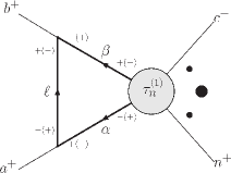
Figure 1: Diagram containing the leading and sub-leading poles as $s_{ab}\to 0$. The axial gauge construction permits the off-shell continuation of the internal legs.

The one-loop:one-loop factorisations involve double poles and we need to determine the sub-leading pieces. By considering a diagram of the form fig. 1 using an axial gauge formalism Kosower:1989xy ; Schwinn:2005pi , we can determine the full pole structure of the rational piece, including the non-factorising simple poles. We have used this approach previously to compute one-loop Dunbar:2010xk ; Alston:2015gea ; Dunbar:2016dgg and two-loop amplitudes Dunbar:2016aux ; Dunbar:2016gjb ; Dunbar:2017nfy ; Dunbar:2019fcq , we labelled this process augmented recursion.

The principal helicity assignment in fig. 1, gives

$$\int\!\!d{\Lambda}^{c}(\alpha^{+},a^{+},b^{+},\beta^{-})\;\tau_{n}^{(1),c}(\alpha^{-},\beta^{+},c^{+},...,n^{+})$$ (48)

where

$$\int\!\!d\Lambda^{c}(\alpha^{+},a^{+},b^{+},\beta^{-})\equiv\frac{i}{c_{\Gamma}(2\pi)^{D}}\int\!\!\frac{d^{D}\ell}{\ell^{2}\alpha^{2}\beta^{2}}{\cal V}_{3}(\alpha,a,\ell){\cal V}_{3}(\ell,b,\beta)\,,$$ (49)

the vertices are in axial gauge and $\tau_{n}^{(1),c}$ is a doubly off-shell current where $c$ denotes an implicit sum over color.

As we are only interested in the residue on the $s_{ab}\to 0$ pole, we do not need the exact current. It is sufficient that the approximate current satisfies two conditions Alston:2015gea ; Dunbar:2016aux :

1. The current contains the leading singularity as $s_{\alpha\beta}\to 0$ with $\alpha^{2},\beta^{2}\neq 0$,

2. The current is the one-loop, single-minus amplitude in the on-shell limit $\alpha^{2},\beta^{2}\to 0$, $s_{\alpha\beta}\neq 0$.

This process is detailed in Dunbar:2017nfy and applied to the full color case in Dunbar:2019fcq .

The $U(N_{c})$ color decomposition of $d\Lambda^{c}$ contains a common kinematic factor so we have the color decompositions

$$\tau_{n}^{(1),c}=\sum_{\lambda}C_{\lambda}\tau^{(1)}_{n:\lambda}\;\;\;{\rm and}\;\;\int d\Lambda^{c}=C_{\Lambda}\int d\Lambda_{0}$$ (50)

where

$$\int d\Lambda_{0}(\alpha^{+},a^{+},b^{+},\beta^{-})=\frac{i}{(2\pi)^{D}}\int\!\!\frac{d^{D}\ell}{\ell^{2}\alpha^{2}\beta^{2}}\frac{[a|\ell|q\rangle[b|\ell|q\rangle}{\left\langle a\,q\right\rangle\left\langle b\,q\right\rangle}\frac{\left\langle\beta\,q\right\rangle^{2}}{\left\langle\alpha\,q\right\rangle^{2}}\,.$$ (51)

Hence the full color contribution is

$$\sum_{\lambda}C_{\Lambda}C_{\lambda}\int\!\!d\Lambda_{0}(\alpha^{+},a^{+},b^{+},\beta^{-})\;\tau_{n:\lambda}^{(1)}(\alpha^{-},\beta^{+},c^{+},\cdots n^{+}).$$ (52)

The various $\tau^{(1)}_{n:\lambda}$ can be expressed as sums of the leading amplitudes $\tau^{(1)}_{n:1}$ via a series of $U(1)$ decoupling identities. For the six-point case there are three currents to calculate. $\tau^{(1)}_{6:1}(\alpha^{-},\beta^{+},c^{+},d^{+},e^{+},f^{+})$ has been calculated previously Dunbar:2016gjb and presented for arbitrary $q$ Dunbar:2017nfy . The remaining two currents are given by

$$\tau^{(1)}_{6:1}(\alpha^{-},c^{+},\beta^{+},d^{+},e^{+},f^{+})$$

$$=\frac{i}{3}\Bigg{(}\frac{\left\langle d\,f\right\rangle\left\langle\alpha\,e\right\rangle^{3}\left[e\,f\right]}{\left\langle c\,\beta\right\rangle\left\langle d\,e\right\rangle^{2}\left\langle e\,f\right\rangle^{2}\left\langle\alpha\,c\right\rangle\left\langle\beta\,d\right\rangle}-\frac{\left\langle\alpha\,d\right\rangle^{3}\left\langle\beta\,e\right\rangle[d|c|\alpha\rangle}{\left\langle c\,\beta\right\rangle\left\langle d\,e\right\rangle^{2}\left\langle e\,f\right\rangle\left\langle f\,\alpha\right\rangle\left\langle\alpha\,c\right\rangle\left\langle\beta\,d\right\rangle^{2}}$$

$$+\frac{[c|d|\alpha\rangle^{3}}{\left\langle e\,f\right\rangle\left\langle f\,\alpha\right\rangle\left\langle\beta\,d\right\rangle^{2}[c|P_{\beta d}|e\rangle t_{c\beta d}}+\frac{[f|c|\alpha\rangle^{3}}{\left\langle c\,\beta\right\rangle\left\langle d\,e\right\rangle^{2}\left\langle\alpha\,c\right\rangle[f|c|\beta\rangle[c|P_{\alpha\beta}|c\rangle}$$

$$+\frac{\left[c\,f\right]^{3}}{\left[f\,\alpha\right]\left[\alpha\,c\right]t_{\beta de}}\times\Bigg{[}\frac{\left[\beta\,e\right]}{\left\langle d\,e\right\rangle\left\langle\beta\,d\right\rangle}+\frac{\left[c\,\beta\right]\left[\beta\,d\right]}{\left\langle d\,e\right\rangle[c|P_{\beta d}|e\rangle}-\frac{\left[d\,e\right]\left[e\,f\right]}{\left\langle\beta\,d\right\rangle[f|c|\beta\rangle}\Bigg{]}\Bigg{)}+\mathcal{O}(s_{\alpha\beta})$$ (53)

and

$$\tau^{(1)}_{6:1}(\alpha^{-},c^{+},d^{+},\beta^{+},e^{+},f^{+})$$

$$=\frac{i}{3}\Bigg{(}-\frac{\left\langle c\,\beta\right\rangle\left\langle\alpha\,d\right\rangle^{3}\left[c\,d\right]}{\left\langle c\,d\right\rangle^{2}\left\langle d\,\beta\right\rangle^{2}\left\langle e\,f\right\rangle\left\langle f\,\alpha\right\rangle\left\langle\beta\,e\right\rangle}+\frac{\left\langle\alpha\,e\right\rangle^{3}\left\langle\beta\,f\right\rangle\left[e\,f\right]}{\left\langle c\,d\right\rangle\left\langle d\,\beta\right\rangle\left\langle e\,f\right\rangle^{2}\left\langle\alpha\,c\right\rangle\left\langle\beta\,e\right\rangle^{2}}$$

$$+\frac{[c|d|\alpha\rangle^{3}}{\left\langle d\,\beta\right\rangle^{2}\left\langle e\,f\right\rangle\left\langle f\,\alpha\right\rangle[c|P_{d\beta}|e\rangle t_{cd\beta}}+\frac{[f|P_{cd}|\alpha\rangle^{3}}{\left\langle c\,d\right\rangle\left\langle\alpha\,c\right\rangle\left\langle\beta\,e\right\rangle^{2}[f|P_{\alpha c}|d\rangle t_{\alpha cd}}$$

$$+\frac{\left[c\,f\right]^{3}}{\left[f\,\alpha\right]\left[\alpha\,c\right]t_{d\beta e}}\times\Bigg{[}\frac{\left[d\,e\right]}{\left\langle d\,\beta\right\rangle\left\langle\beta\,e\right\rangle}+\frac{\left[c\,d\right]\left[d\,\beta\right]}{\left\langle\beta\,e\right\rangle[c|P_{d\beta}|e\rangle}-\frac{\left[e\,f\right]\left[\beta\,e\right]}{\left\langle d\,\beta\right\rangle[f|P_{\alpha c}|d\rangle}\Bigg{]}\Bigg{)}+\mathcal{O}(s_{\alpha\beta}).$$ (54)

Many of the terms in the non-adjacent currents don’t give rationals upon integration. We are thus left with

$$\int\!\!\frac{d^{D}\ell}{\ell^{2}\alpha^{2}\beta^{2}}\frac{i}{(2\pi)^{D}}\frac{[a|\ell|q\rangle[b|\ell|q\rangle}{\left\langle a\,q\right\rangle\left\langle b\,q\right\rangle}\tau^{(1)}_{6:1}(\alpha^{-},c^{+},\beta^{+},d^{+},e^{+},f^{+})|_{\mathbb{Q}}$$

$$=\frac{i}{6}\frac{\left[a\,b\right]}{\left\langle a\,b\right\rangle}\Bigg{(}\frac{\left\langle d\,f\right\rangle\left\langle a\,e\right\rangle^{3}\left[e\,f\right]\left\langle b\,q\right\rangle^{2}}{\left\langle c\,b\right\rangle\left\langle d\,e\right\rangle^{2}\left\langle e\,f\right\rangle^{2}\left\langle a\,c\right\rangle\left\langle b\,d\right\rangle\left\langle a\,q\right\rangle^{2}}-\frac{\left\langle a\,d\right\rangle^{3}\left\langle b\,e\right\rangle[d|c|a\rangle\left\langle b\,q\right\rangle^{2}}{\left\langle c\,b\right\rangle\left\langle d\,e\right\rangle^{2}\left\langle e\,f\right\rangle\left\langle f\,a\right\rangle\left\langle a\,c\right\rangle\left\langle b\,d\right\rangle^{2}\left\langle a\,q\right\rangle^{2}}$$

$$+\frac{[f|c|a\rangle^{3}\left\langle b\,q\right\rangle^{2}}{\left\langle c\,b\right\rangle\left\langle d\,e\right\rangle^{2}\left\langle a\,c\right\rangle\left\langle a\,q\right\rangle^{2}[f|c|b\rangle[c|P_{ab}|c\rangle}\Bigg{)}$$ (55)

and

$$\int\!\!\frac{d^{D}\ell}{\ell^{2}\alpha^{2}\beta^{2}}\frac{i}{(2\pi)^{D}}\frac{[a|\ell|q\rangle[b|\ell|q\rangle}{\left\langle a\,q\right\rangle\left\langle b\,q\right\rangle}\tau^{(1)}_{6:1}(\alpha^{-},c^{+},d^{+},\beta^{+},e^{+},f^{+})|_{\mathbb{Q}}$$

$$=\frac{i}{6}\frac{\left[a\,b\right]}{\left\langle a\,b\right\rangle}\Bigg{(}\frac{\left\langle a\,e\right\rangle^{3}\left\langle b\,f\right\rangle\left\langle b\,q\right\rangle^{2}\left[e\,f\right]}{\left\langle c\,d\right\rangle\left\langle d\,b\right\rangle\left\langle e\,f\right\rangle^{2}\left\langle a\,c\right\rangle\left\langle a\,q\right\rangle^{2}\left\langle b\,e\right\rangle^{2}}-\frac{\left\langle c\,b\right\rangle\left\langle b\,q\right\rangle^{2}\left\langle a\,d\right\rangle^{3}\left[c\,d\right]}{\left\langle c\,d\right\rangle^{2}\left\langle d\,b\right\rangle^{2}\left\langle e\,f\right\rangle\left\langle f\,a\right\rangle\left\langle a\,q\right\rangle^{2}\left\langle b\,e\right\rangle}\Bigg{)}.$$ (56)

We then color-dress fig. 1, sum over all distinct diagrams, extract the contribution to each color structure and take the residues. Summing over all the channels excited by the Risager shift and all helicities gives the full color two-loop amplitude.

References

• (1) Les Houches 2017: Physics at TeV Colliders Standard Model Working Group Report, 2018.
• (2) P. Azzi et al., “Report from Working Group 1,” CERN Yellow Rep. Monogr., vol. 7, pp. 1–220, 2019.
• (3) S. Caron-Huot, L. J. Dixon, F. Dulat, M. von Hippel, A. J. McLeod, and G. Papathanasiou, “Six-Gluon amplitudes in planar $\mathcal{N}$ = 4 super-Yang-Mills theory at six and seven loops,” JHEP, vol. 08, p. 016, 2019.
• (4) J. L. Bourjaily, E. Herrmann, C. Langer, A. J. McLeod, and J. Trnka, “All-Multiplicity Non-Planar MHV Amplitudes in sYM at Two Loops,” 2019.
• (5) E. W. N. Glover, C. Oleari, and M. E. Tejeda-Yeomans, “Two loop QCD corrections to gluon-gluon scattering,” Nucl. Phys., vol. B605, pp. 467–485, 2001.
• (6) Z. Bern, A. De Freitas, and L. J. Dixon, “Two loop helicity amplitudes for gluon-gluon scattering in QCD and supersymmetric Yang-Mills theory,” JHEP, vol. 03, p. 018, 2002.
• (7) T. Ahmed, J. Henn, and B. Mistlberger, “Four-particle scattering amplitudes in QCD at NNLO to higher orders in the dimensional regulator,” JHEP, vol. 12, p. 177, 2019.
• (8) S. Badger, H. Frellesvig, and Y. Zhang, “A Two-Loop Five-Gluon Helicity Amplitude in QCD,” JHEP, vol. 12, p. 045, 2013.
• (9) S. Badger, G. Mogull, A. Ochirov, and D. O’Connell, “A Complete Two-Loop, Five-Gluon Helicity Amplitude in Yang-Mills Theory,” JHEP, vol. 10, p. 064, 2015.
• (10) T. Gehrmann, J. M. Henn, and N. A. Lo Presti, “Analytic form of the two-loop planar five-gluon all-plus-helicity amplitude in QCD,” Phys. Rev. Lett., vol. 116, no. 6, p. 062001, 2016. [Erratum: Phys. Rev. Lett.116,no.18,189903(2016)].
• (11) D. C. Dunbar and W. B. Perkins, “Two-loop five-point all plus helicity Yang-Mills amplitude,” Phys. Rev., vol. D93, no. 8, p. 085029, 2016.
• (12) S. Badger, C. Brønnum-Hansen, H. B. Hartanto, and T. Peraro, “Analytic helicity amplitudes for two-loop five-gluon scattering: the single-minus case,” JHEP, vol. 01, p. 186, 2019.
• (13) S. Abreu, J. Dormans, F. Febres Cordero, H. Ita, B. Page, and V. Sotnikov, “Analytic Form of the Planar Two-Loop Five-Parton Scattering Amplitudes in QCD,” JHEP, vol. 05, p. 084, 2019.
• (14) S. Badger, D. Chicherin, T. Gehrmann, G. Heinrich, J. M. Henn, T. Peraro, P. Wasser, Y. Zhang, and S. Zoia, “Analytic form of the full two-loop five-gluon all-plus helicity amplitude,” Phys. Rev. Lett., vol. 123, no. 7, p. 071601, 2019.
• (15) D. C. Dunbar, G. R. Jehu, and W. B. Perkins, “Two-loop six gluon all plus helicity amplitude,” Phys. Rev. Lett., vol. 117, no. 6, p. 061602, 2016.
• (16) D. C. Dunbar, J. H. Godwin, G. R. Jehu, and W. B. Perkins, “Analytic all-plus-helicity gluon amplitudes in QCD,” Phys. Rev., vol. D96, no. 11, p. 116013, 2017.
• (17) D. C. Dunbar, W. B. Perkins, and J. M. W. Strong, “An $n$-point QCD two-loop amplitude,” 2020.
• (18) S. D. Alston, D. C. Dunbar, and W. B. Perkins, “Complex Factorisation and Recursion for One-Loop Amplitudes,” Phys. Rev., vol. D86, p. 085022, 2012.
• (19) A. C. Edison and S. G. Naculich, “SU(N) group-theory constraints on color-ordered five-point amplitudes at all loop orders,” Nucl. Phys., vol. B858, pp. 488–501, 2012.
• (20) A. C. Edison and S. G. Naculich, “Symmetric-group decomposition of SU(N) group-theory constraints on four-, five-, and six-point color-ordered amplitudes,” JHEP, vol. 09, p. 069, 2012.
• (21) S. Catani, “The Singular behavior of QCD amplitudes at two loop order,” Phys. Lett., vol. B427, pp. 161–171, 1998.
• (22) Z. Kunszt, A. Signer, and Z. Trocsanyi, “Singular terms of helicity amplitudes at one loop in QCD and the soft limit of the cross-sections of multiparton processes,” Nucl. Phys., vol. B420, pp. 550–564, 1994.
• (23) D. C. Dunbar, J. H. Godwin, W. B. Perkins, and J. M. W. Strong, “Color Dressed Unitarity and Recursion for Yang-Mills Two-Loop All-Plus Amplitudes,” Phys. Rev., vol. D101, no. 1, p. 016009, 2020.
• (24) D. C. Dunbar, G. R. Jehu, and W. B. Perkins, “The two-loop n-point all-plus helicity amplitude,” Phys. Rev., vol. D93, no. 12, p. 125006, 2016.
• (25) J. Henn, B. Power, and S. Zoia, “Conformal Invariance of the One-Loop All-Plus Helicity Scattering Amplitudes,” 2019.
• (26) R. Britto, F. Cachazo, B. Feng, and E. Witten, “Direct proof of tree-level recursion relation in Yang-Mills theory,” Phys. Rev. Lett., vol. 94, p. 181602, 2005.
• (27) K. Risager, “A Direct proof of the CSW rules,” JHEP, vol. 12, p. 003, 2005.
• (28) S. Badger, G. Mogull, and T. Peraro, “Local integrands for two-loop all-plus Yang-Mills amplitudes,” JHEP, vol. 08, p. 063, 2016.
• (29) D. A. Kosower, “Light Cone Recurrence Relations for QCD Amplitudes,” Nucl. Phys., vol. B335, pp. 23–44, 1990.
• (30) C. Schwinn and S. Weinzierl, “Scalar diagrammatic rules for Born amplitudes in QCD,” JHEP, vol. 05, p. 006, 2005.
• (31) D. C. Dunbar, J. H. Ettle, and W. B. Perkins, “Augmented Recursion For One-loop Gravity Amplitudes,” JHEP, vol. 06, p. 027, 2010.
• (32) S. D. Alston, D. C. Dunbar, and W. B. Perkins, “$n$-point amplitudes with a single negative-helicity graviton,” Phys. Rev., vol. D92, no. 6, p. 065024, 2015.
• (33) D. C. Dunbar and W. B. Perkins, “${\cal N}=4$ supergravity next-to-maximally-helicity-violating six-point one-loop amplitude,” Phys. Rev., vol. D94, no. 12, p. 125027, 2016.