On the Numerical Analysis and Visualisation of Implicit Ordinary Differential Equations

Abstract

We discuss how the geometric theory of differential equations can be used for the numerical integration and visualisation of implicit ordinary differential equations, in particular around singularities of the equation. The Vessiot theory automatically transforms an implicit differential equation into a vector field distribution on a manifold and thus reduces its analysis to standard problems in dynamical systems theory like the integration of a vector field and the determination of invariant manifolds. For the visualisation of low-dimensional situations we adapt the streamlines algorithm of Jobard and Lefer to 2.5 and 3 dimensions. A concrete implementation in Matlab is discussed and some concrete examples are presented.

1. Introduction

Most textbooks on the theoretical or the numerical analysis of ordinary differential equations assume that the equations are given in the solved form $\mathbf{u}^{(q)}=\mathbf{f}(t,\mathbf{u},\dot{\mathbf{u}},\dots,\mathbf{u}^{(q-1)})$. Fully implicit differential equations $\mathbf{F}(t,\mathbf{u},\dot{\mathbf{u}},\dots,\mathbf{u}^{(q)})=0$ exhibit a much wider range of behaviours including the appearance of singularities. Even basic questions of the existence and uniqueness of solutions are much more involved for them and near singularities basically all numerical methods break down or become at least ill-conditioned. In this article, we demonstrate how a geometric approach allows to translate many of these questions into standard problems for dynamical systems on manifolds.

Our approach to implicit equations is based on the Vessiot distribution associated to any differential equation (see [10, 17] and references therein) and was already employed in [12, 18]. In the case of a not underdetermined ordinary differential equation (which we will exclusively consider in this article), the Vessiot distribution is almost everywhere one-dimensional and can thus be locally represented by a vector field. One-dimensional integral curves of this vector field correspond to generalised solutions which around regular points are nothing but the prolongation of classical solutions. Irregular singularities become stationary points and the local solution behaviour around them is determined by their invariant manifolds.

In this article, we will describe the ideas underlying a suite of Matlab routines (developed as part of the first author’s master thesis [4]) that allow (i) for the automated numerical determination and integration of the Vessiot distribution wherever it is one-dimensional, (ii) for the visualisation of the streamlines of the Vessiot distribution in 2, 2.5 and 3 dimensions using a method proposed by Jobard and Lefer [11] and (iii) for the numerical determination of invariant manifolds and the reduced dynamics on them via an approach developed by Beyn and Kleß [3] and later improved by Eirola and von Pfaler [8].

The article is structured as follows. The next section recalls the basic ingredients of the geometric theory of ordinary differential equations: jet bundles, Vessiot spaces, singularities and generalised solutions. Section 3 is concerned with the numerical integration away from irregular singularities which boils down to integrating a vector field on a manifold. The analysis of the local solution behaviour around irregular singularities using invariant manifolds of stationary points is the topic of Section 4. The following section describes our ansatz for visualising streamlines in various dimensions. In Section 6, two concrete examples of a fully nonlinear first-order and of a quasi-linear second-order equation are treated. The reader may find it useful to refer from time to time to this section, as any concept or construction discussed in earlier sections will be explicitly demonstrated there. Finally, some conclusions are given.

2. Geometry of Differential Equations

Differential equations are geometrically modelled via jet bundles [13, 15, 16, 17]. Let $\pi:\mathcal{E}\rightarrow\mathcal{T}$ be a fibred manifold with $\dim{\mathcal{T}}=1$ for ordinary differential equations, e. g. $\mathcal{T}=\mathbbm{R}$ and $\mathcal{E}=\mathcal{T}\times\mathbbm{R}^{m}$ with $\pi$ the canonical projection on $\mathcal{T}$. For simplicity, we work in local coordinates, although we use throughout a “global notation”. As coordinate on the base space $\mathcal{T}$ we use $t$ and fibre coordinates in the total space $\mathcal{E}$ will be $\mathbf{u}=(u^{1},\ldots,u^{m})$. The first derivative of $u^{\alpha}$ will be denoted by $\dot{u}^{\alpha}$; higher derivatives are written in the form $u^{\alpha}_{k}=d^{k}u^{\alpha}/dt^{k}$. Adding all derivatives $u^{\alpha}_{k}$ with $k\leq q$ (collectively denoted by $\mathbf{u}_{(q)}$) defines a coordinate system for the $q$-th order jet bundle $J_{q}\pi$. There are natural fibrations $\pi^{q}_{r}:J_{q}\pi\rightarrow J_{r}\pi$ for $r<q$ and $\pi^{q}:J_{q}\pi\rightarrow\mathcal{T}$ “forgetting” all higher derivatives. Sections $\sigma:\mathcal{T}\rightarrow\mathcal{E}$ of the fibration $\pi$ correspond to functions $\mathbf{u}=\mathbf{s}(t)$, as locally they can always be written in the form of a graph $\sigma(t)=\bigl{(}t,\mathbf{s}(t)\bigr{)}$. To such a section $\sigma$, we associate its prolongation $j_{q}\sigma:\mathcal{T}\rightarrow J_{q}\pi$, a section of the fibration $\pi^{q}$ given by $j_{q}\sigma(t)=\bigl{(}t,\mathbf{s}(t),\dot{\mathbf{s}}(t),\ddot{\mathbf{s}}(t),\dots\bigr{)}$.

The geometry of the $q$-th order jet bundle $J_{q}\pi$ is to a large extent determined by its contact structure describing intrinsically the relationship between the different types of coordinates. The contact distribution is the smallest distribution $\mathcal{C}_{q}\subset T(J_{q}\pi)$ that contains the tangent spaces $T(\operatorname{im}{j_{q}\sigma})$ of all $q$ times prolonged sections and any field in it is a contact vector field. In local coordinates, $\mathcal{C}_{q}$ is generated by one transversal and $m$ vertical fields (with respect to $\pi^{q}$):

$$C_{\mathrm{trans}}^{(q)} =\partial_{t}+\sum_{j=0}^{q-1}u^{\alpha}_{j+1}\partial_{u^{\alpha}_{j}}\;,$$ (1a)

$$C^{(q)}_{\alpha} =\partial_{u^{\alpha}_{q}}\;,\qquad 1\leq\alpha\leq m\;.$$ (1b)

Proposition 1.

A section $\gamma:\mathcal{T}\rightarrow J_{q}\pi$ is of the form $\gamma=j_{q}\sigma$ with $\sigma:\mathcal{T}\rightarrow\mathcal{E}$, if and only if $T_{\gamma(t)}(\operatorname{im}{\gamma})\subseteq\mathcal{C}_{q}|_{\gamma(t)}$ for all points $t\in\mathcal{T}$ where $\gamma$ is defined.

Compared with the usual intrinsic geometric definition of a differential equation, ours allows for certain types of singularities, as it imposes considerably weaker conditions on the restricted projection $\hat{\pi}^{q}$ which in the standard definition must be a surjective submersion. Note that we do not distinguish between scalar equations and systems.

Definition 2.

An (ordinary) differential equation of order $q$ is a submanifold $\mathcal{R}_{q}\subseteq J_{q}\pi$ such that the restriction $\hat{\pi}^{q}$ of the projection $\pi^{q}:J_{q}\pi\rightarrow\mathcal{T}$ to $\mathcal{R}_{q}$ has a dense image in $\mathcal{T}$. A (strong) solution is a (local) section $\sigma:\mathcal{T}\rightarrow\mathcal{E}$ such that $\operatorname{im}{j_{q}\sigma}\subseteq\mathcal{R}_{q}$.

Locally, a differential equation $\mathcal{R}_{q}\subseteq J_{q}\pi$ can be described as the zero set of some smooth functions $\Phi:J_{q}\pi\rightarrow\mathbbm{R}$ which brings us back to the usual picture of a differential equation. Checking whether a function $\mathbf{s}(t)$ is a solution by entering it and its derivatives into $\Phi$ corresponds to verifying that $\operatorname{im}{j_{q}\sigma}\subseteq\mathcal{R}_{q}$ for the section $\sigma$ defined by $\mathbf{s}(t)$. In the sequel, we will always assume that we are dealing with a formally integrable equation, i. e. that there are no hidden integrability conditions. We refer to [17] for more details on the meaning and the effective verification of this assumption. Furthermore, we will assume throughout that all considered differential equations are not underdetermined, i. e. their general solution depends only on a finite number of constants.

A key insight of Cartan was to study infinitesimal solutions or integral elements of a differential equation $\mathcal{R}_{q}\subseteq J_{q}\pi$, i. e. to consider at any point $\rho\in\mathcal{R}_{q}$ those linear subspaces $\mathcal{U}_{\rho}\subseteq T_{\rho}\mathcal{R}_{q}$ which are potentially the tangent space at $\rho$ of a prolonged solution through $\rho$. We will follow here an approach pioneered by Vessiot [23] which is based on vector fields and dual to the more popular Cartan-Kähler theory of exterior differential systems (see [9, 10, 17] for modern presentations). By Proposition 1, the tangent spaces $T_{\rho}(\operatorname{im}{j_{q}\sigma})$ of prolonged sections at points $\rho\in J_{q}\pi$ are always subspaces of the contact distribution $\mathcal{C}_{q}|_{\rho}$. If the section $\sigma$ is a solution of $\mathcal{R}_{q}$, it furthermore satisfies $\operatorname{im}{j_{q}\sigma}\subseteq\mathcal{R}_{q}$ by Definition 2 and hence $T_{\rho}(\operatorname{im}{j_{q}\sigma})\subseteq T_{\rho}\mathcal{R}_{q}$ for any point $\rho\in\operatorname{im}{j_{q}\sigma}$. These considerations motivate the following construction.

Definition 3.

The Vessiot space of the differential equation $\mathcal{R}_{q}\subseteq J_{q}\pi$ at the point $\rho\in\mathcal{R}_{q}$ is that part of the contact distribution that lies tangential to $\mathcal{R}_{q}$, i. e. the vector space

$$\mathcal{V}_{\rho}[\mathcal{R}_{q}]=T_{\rho}\mathcal{R}_{q}\cap\mathcal{C}_{q}|_{\rho}\;.$$ (2)

The family of all Vessiot spaces of a differential equation $\mathcal{R}_{q}$ is its Vessiot distribution $\mathcal{V}[\mathcal{R}_{q}]$.

Our discussion of the explicit construction of the Vessiot spaces in the next section will show that they are almost everywhere one-dimensional (because of our restriction to not underdetermined equations) and that they define on an open subset of $\mathcal{R}_{q}$ a smooth regular distribution. Following the terminology of Arnold [1], we will distinguish the points on $\mathcal{R}_{q}$ according to the properties of their Vessiot spaces.

Definition 4.

A point $\rho\in\mathcal{R}_{q}$ is regular, if $\dim{\mathcal{V}_{\rho}[\mathcal{R}_{q}]}=1$ and $\mathcal{V}_{\rho}[\mathcal{R}_{q}]$ is transversal relative to the fibration $\pi^{q}$. If $\dim{\mathcal{V}_{\rho}[\mathcal{R}_{q}]}=1$, but $\mathcal{V}_{\rho}[\mathcal{R}_{q}]$ is vertical, then $\rho$ is a regular singularity. Points where $\dim{\mathcal{V}_{\rho}[\mathcal{R}_{q}]}>1$ are called irregular singularities.

It is not difficult to show that the regular points form a dense subset and at them the classical existence and uniqueness theorems for differential equations hold (see e. g. the discussion in [12]). At singularities, one typically looses in particular the uniqueness – there can be anything from two to infinitely many one-sided solutions – and the existence of two-sided solutions going through the point can become a highly non-trivial problem. Conventional numerical integrators will break down when approaching such points. For an analysis of the solution behaviour in their neighbourhood, we need the following, more general notions of solutions.

Definition 5.

A generalised solution of the differential equation $\mathcal{R}_{q}$ is an integral curve $\mathcal{N}\subseteq\mathcal{R}_{q}$ of the Vessiot distribution $\mathcal{V}[\mathcal{R}_{q}]$, i. e. a one-dimensional submanifold such that $T_{\rho}\mathcal{N}\subseteq\mathcal{V}_{\rho}[\mathcal{R}_{q}]$ at every point $\rho\in\mathcal{N}$. The projection $\pi_{0}^{q}(\mathcal{N})\subset\mathcal{E}$ is called a geometric solution.

Generalised solutions live in the jet bundle $J_{q}\pi$ and not in the base manifold $\mathcal{E}$. If a section $\sigma$ defines a strong solution in the sense of Definition 2, then $\operatorname{im}{j_{q}\sigma}\subseteq\mathcal{R}_{q}$ is a generalised solution and $\operatorname{im}{\sigma}\subset\mathcal{E}$ the corresponding geometric solution. However, not all geometric solutions are graphs of functions. In fact, they are not even necessarily smooth curves, as they arise via a projection.

Away from the irregular singularities, the Vessiot distribution can be locally generated by a vector field. In [12], it is shown that the irregular singularities are stationary points of this vector field. Thus the analysis of an implicit differential equation satisfying our assumptions can be reduced to the study of an autonomous dynamical system on the submanifold $\mathcal{R}_{q}\subset J_{q}\pi$. In the next section we will discuss how this idea can be realised numerically.

In this approach, regular singularities play no role at all. There goes a unique generalised solution through any regular singularity and the singularity is a smooth point of this curve [12]. The singular character of such a point becomes apparent only, if one tries to interpret the obtained curve as the prolongation of the graph of a function, as this is usually not possible. Indeed, if one considers the associated geometric solution, it usually exhibits a cusp underneath the regular singularity. However, this does not affect in the least the numerical determination of the generalised solution.

3. Numerical Integration of Implicit Differential Equations

Classical approaches essentially transform numerically an implicit equation into either an explicit differential equation or a differential algebraic equation which is then solved by standard methods. Such approaches run into difficulties whenever the integration gets close to a singularity, as at singularities the ranks of certain crucial matrices jump and thus already in their vicinity condition numbers deterioriate. Furthermore, at singularities solutions are no longer unique and the number of solutions can be anything from two to infinity.

We describe now a realisation of a different approach, namely the numerical integration of the Vessiot distribution or more precisely, of a vector field locally generating it (essentially the same approach was already used by Tuomela [21, 22]). Thus we determine directly generalised solutions. This approach has some advantages. In particular, it immediately resolves the problem of regular singularities, as we already discussed above. Equations of arbitrary high order can be tackled directly without the need to rewrite them as first-order equations (in fact, in this approach such a rewriting would lead to unnecessary large equations). Finally, we will show that also the analysis of irregular singularities can be supported by standard methods from dynamical systems theory, although this remains a hard problem for larger systems.

The price to pay for these advantages is an increase in the system size. If the original implicit system involves $m$ unknown functions and $k$ equations of maximal order $q$, then we have to deal with an autonomous vector field in $(q+1)m+1$ unknown functions plus $k$ weak invariants of this field. For moderate values of $m$ and $q$, which we will exclusively consider in this article, this increase is easily tolerable in view of the advantages. For larger systems, one could think of a combination of the classical approach (away from the singularities) and the here described approach (in the vicinity of singularities) to improve efficiency.

Let the differential equation $\mathcal{R}_{q}\subset J_{q}\pi$ be described by the implicit system $\mathbf{F}(t,\mathbf{u}_{(q)})=0$. We want to approximate the unique generalised solution starting at a given point $\rho^{(0)}\in\mathcal{R}_{q}$ which is not an irregular singularity. We construct numerically a vector field $X$ for which this solution is a trajectory and integrate it numerically obtaining a sequence of points $\rho^{(i)}$. From the discussion in the previous section, it is obvious that the value $X_{\rho}$ of $X$ at some point $\rho$ on the generalised solution generates the Vessiot space $\mathcal{V}_{\rho}[\mathcal{R}_{q}]$. Therefore, having arrived at some point $\rho^{(n)}$, the first task for constructing $\rho^{(n+1)}$ consists of determining $\mathcal{V}_{\rho^{(n)}}[\mathcal{R}_{q}]$.

Computing the Vessiot space $\mathcal{V}_{\rho^{(n)}}[\mathcal{R}_{q}]$ at a point $\rho^{(n)}\in\mathcal{R}_{q}$ is straightforward and requires in principle only linear algebra. Any vector $X_{\rho^{(n)}}\in\mathcal{V}_{\rho^{(n)}}[\mathcal{R}_{q}]$ lies in the contact distribution $\mathcal{C}^{(q)}|_{\rho^{(n)}}$ and thus can be written as a linear combination of the basic contact fields given in (1): $X_{\rho^{(n)}}=aC^{(q)}_{\mathrm{trans}}|_{\rho^{(n)}}+\mathbf{b}\mathbf{C}^{(q)}|_{\rho^{(n)}}$. On the other hand, $X_{\rho^{(n)}}$ must be tangent to $\mathcal{R}_{q}$. Hence, $X_{\rho^{(n)}}$ must satisfy the equations $d\mathbf{F}|_{\rho^{(n)}}(X_{\rho^{(n)}})=0$. Evaluation of this condition yields the following homogeneous linear system of equations for the coefficients $a$, $\mathbf{b}$:

$$C^{(q)}_{\mathrm{trans}}(\mathbf{F})(\rho^{(n)})a+\mathbf{C}^{(q)}(\mathbf{F})(\rho^{(n)})\mathbf{b}=0\,.$$ (3)

By studying the ranks of the full coefficient matrix of this system and of the submatrix $\mathbf{C}^{(q)}(\mathbf{F})(\rho^{(n)})$ one can easily detect whether $\rho^{(n)}$ is a singularity and if yes, what kind (see e. g. [12]).

At a given point $\rho^{(n)}\in\mathcal{R}_{q}$, it is straightforward to determine a basis of the solution space of (3) with standard numerical methods. Away from the irregular singularities, this basis consists of a single vector $\tilde{X}_{\rho^{(n)}}$ generating $\mathcal{V}_{\rho^{(n)}}[\mathcal{R}_{q}]$. To enhance the stability of the numerical integration of $X$, we normalise this vector to unit length and obtain the desired vector $X_{\rho^{(n)}}$. In our implementation, the norm condition is actually added to the linear system (3). On one side, this makes the system nonlinear, but on the other side it also makes it square and thus easily solvable by a Newton method. This idea also helps to overcome another problem: if $X_{\rho^{(n)}}$ is a unit length solution of (3), then the same holds for $-X_{\rho^{(n)}}$. Thus if one is careless, it may happen that one integrates the same piece of the trajectory back and forth. For the solution of the square nonlinear system, we always take $X_{\rho^{(n-1)}}$ as starting value for the Newton iteration. For reasonably small step sizes, $X_{\rho^{(n)}}$ and $X_{\rho^{(n-1)}}$ will not differ much so that we will obtain rapid convergence to the right vector.

Remark 6.

For smaller systems, the linear system (3) could be tackled symbolically treating the point $\rho^{(n)}\in\mathcal{R}_{q}$ as a parameter. As the behaviour of the system generally depends on the point $\rho^{(n)}$, one faces the nontrivial problem of solving a parametric linear system with potentially many necessary case distinctions. A method for this was presented by Sit [20] and it is also possible to use a Thomas decomposition (see e. g. [2] and references therein). Both approaches require that the parameter dependency is polynomial and are computationally quite demanding. We will use the second approach elsewhere for the development of an effective theory of algebraic differential equations. In this work, we will restrict to a purely numerical approach.

While the linear system (3) can be written down for any point $\rho\in J_{q}\pi$, it is actually defined only on the submanifold $\mathcal{R}_{q}\subset J_{q}\pi$. If a parametrisation of this submanifold is known, then one could rewrite the system and the vector field it describes in these parameters. However, in practise such a parametrisation is often not available. Therefore we prefer to work with the jet coordinates on $J_{q}\pi$ and thus with redundant coordinates. During the numerical integration, we must then ensure that our approximate solution stays on the submanifold $\mathcal{R}_{q}\subset J_{q}\pi$.

More precisely, our approach leads to the numerical integration of the autonomous system

$$t^{\prime}=a(t,\mathbf{u}_{(q)}),\ \ \mathbf{u}^{\prime}=a(t,\mathbf{u}_{(q)})\dot{\mathbf{u}},\ \ \dots\ \ \mathbf{u}^{\prime}_{i}=a(t,\mathbf{u}_{(q)})\mathbf{u}_{i+1},\ \ \dots\ \ \mathbf{u}_{q}^{\prime}=\mathbf{b}(t,\mathbf{u}_{(q)})$$ (4)

where ^′ denotes the derivative with respect to some variable $x$ parametrising our generalised solution, all variables $t,\mathbf{u}_{(q)}$ are considered as independent algebraic variables and the functions $a$, $\mathbf{b}$ arise from solving the linear system (3). However, we are only interested in solutions of (4) which lie on the manifold $\mathcal{R}_{q}$, i. e. we have the additional algebraic constraints $\mathbf{F}(t,\mathbf{u}_{(q)})=0$. By construction, these constraints represent weak invariants of (4), since the vector field $X$ is everywhere tangential to the manifold $\mathcal{R}_{q}$.

Hence we combined a standard numerical integrator applied to (4) with a subsequent projection on the manifold $\mathcal{R}_{q}$ (if the obtained point $\rho^{(n+1)}$ lies too far away). Such projections are well-studied in numerical analysis and it is well-known that they do not affect the convergence order of the numerical integrator. Note furthermore that solving (3) at a point $\rho$ satisfying $\mathbf{F}(\rho)=\epsilon$ will lead to a vector which is tangential to the manifold described by the perturbed system $\mathbf{F}(t,\mathbf{u}^{(q)})=\epsilon$. This observation implies that numerical errors will not lead to a strong drift off $\mathcal{R}_{q}$. In fact, in many situations the manifold $\mathcal{R}_{q}$ will even be orbitally stable for the dynamical system (4). Indeed, we never observed any numerical problems due to a drift.

4. Solutions at Irregular Singularities

As already mentioned above, irregular singularities become stationary points of the vector field $X$ describing the Vessiot distribution locally in their neighbourhood. Generalised solutions through the singularity may then be interpreted as one-dimensional invariant manifolds of this vector field containing the singularity. Hence for the analysis of the local solution behaviour near an irregular singularity it is useful to compute the invariant manifolds at the stationary point.

A more or less automated complete analysis of an irregular singularity is in general only possible in certain low-dimensional situations. If the singularity corresponds to an hyperbolic stationary point, then the dimension plays no role. A complete analysis of this case will appear in [19]. However, singularities correspond rarely to hyperbolic stationary points (in the case of scalar higher-order equations it is even impossible that a hyperbolic stationary point arises). If the centre manifold at a non-hyperbolic stationary point is at most two-dimensional, then a complete analysis is possible using first a centre manifold reduction to a two-dimensional system and then blow-ups [7] (and there even exist computer programmes for this task like P4 described in [7]).

The simplest situation arises, if an (un)stable or centre manifold is one-dimensional. In this case, it can immediately be identified with a generalised solution through the stationary point. If an invariant manifold is higher dimensional, then one must analyse in more details the reduced dynamics on it. The key question is whether or not it is possible to combine two trajectories approaching the singularity with the same tangent to a smooth invariant manifold. Assume for example that we are dealing with a two-dimensional invariant manifold on which the phase portrait looks like a node with two tangents. Then almost all trajectories will approach the singularity tangent to the eigenvector corresponding to the eigenvalue whose real part has the smaller absolute value. If this eigenvector is transversal to the fibration $\pi^{q}$, then we obtain generalised solutions through the singularity which correspond to smooth classical solutions. Otherwise, the classical solutions are of finite regularity.

Remark 7.

Centre manifolds lead to further challenges. It is well known that a centre manifold is not necessarily unique. In fact, if we one has e. g. a saddle node, then there is a unique centre manifold on one side of the singularity and infinitely many centre manifolds on the other side. In dynamical systems theory, one usually considers different centre manifolds as equivalent, as they are exponentially close when approach the singularity. For us, each centre manifold corresponds to a different generalised solution and all of them are of interest. Thus the analysis of the singularity requires in such a case precise statements about the (non-)uniqueness and the regularity of the centre manifolds which are not so easy to obtain.

A complete analysis is always possible for a first-order scalar equation $\mathcal{R}_{1}\subset J_{1}\pi$. In this case, the Vessiot distribution induces a dynamical system on the two-dimensional manifold $\mathcal{R}_{1}$ and all its stationary points can be studied using the methods described in [7]. A concrete example is considered in Section 6. For higher-order scalar equations $\mathcal{R}_{q}\subset J_{q}\pi$, one obtains a dynamical system on a $(q+1)$-dimensional manifold and it is easy to see that no stationary point of it can be hyperbolic, as the $q-1$ “middle rows” of the Jacobian are multiples of the first row. Hence we obtain many zero eigenvalues.

Remark 8.

It was shown in [18] that quasi-linear equations have their own theory (see also the forthcoming work [19] for a much more extensive treatment of this special case). Given a quasi-linear equation $\mathcal{R}_{q}\subset J_{q}\pi$, one may consider instead of the Vessiot distribution on $\mathcal{R}_{q}$ its well-defined projection into $J_{q-1}\pi$. Furthermore, this projection is usually extendable to the whole jet bundle $J_{q-1}\pi$ which leads to further phenomena specific to quasi-linear equations. This projectability simplifies the analysis in the sense that there is no longer the need to work with redundant coordinates in an ambient space. Otherwise, the analysis is performed along the same lines as for fully nonlinear systems by studying the stationary points of the projected Vessiot distribution which we call impasse points to distinguish them from the singularities living one order higher. A concrete example of a quasi-linear second-order equation will be studied in Section 6.

For the computation of invariant manifolds, we implemented an algorithm for the construction of a Taylor series approximation of the invariant manifold originally developed by Beyn and Kleß [3] and later improved by Eirola and von Pfaler [8]. Consider an $n$-dimensional autonomous dynamical system $\dot{\mathbf{x}}=\mathbf{f}(\mathbf{x})$ with a stationary point $\xi\in\mathbbm{R}^{n}$. Assume that the spectrum of the Jacobian $J(\xi)$ of $\mathbf{f}$ in $\xi$ can be disjointly split into two parts, $\mathrm{Spec}\bigl{(}J(\xi)\bigr{)}=\Sigma\sqcup\tilde{\Sigma}$, with a corresponding splitting into generalised eigenspaces $\mathbbm{R}^{n}=E\oplus\tilde{E}$. It is well known that then, under certain gap conditions, an invariant manifold $W$ exists which is tangent to $E$ and which can locally be written as a graph over some neighbourhood $U$ of the origin in $E$: $W=\bigl{\{}(\mathbf{y},\mathbf{h}(\mathbf{y}))\mid\mathbf{y}\in U\subseteq E\bigr{\}}$. Furthermore, the reduced dynamics on $W$ is given by an autonomous system $\dot{\mathbf{y}}=\mathbf{g}(\mathbf{y})$ of dimension $\dim{E}$. The goal is the construction of a Taylor series approximation of $\mathbf{h}$ and consequently of $\mathbf{g}$. Beyn and Kleß [3] showed how this problem can be reduced to solving multilinear Sylvester equations; in the subsequent improvement by Eirola and von Pfaler [8], solving standard Sylvester equations is sufficient. Our implementation uses for this the built-in Matlab procedure.

It should be noted that our implementation does not check whether appropriate gap conditions are indeed satisfied and thus an invariant manifold of sufficiently high regularity really exists. This is the responsibility of the user. In our current implementation, it is only possible to determine Taylor series up to degree 10. The reason is simply that certain combinatorial coefficients always appearing in the computations independent of the concrete dynamical system considered have been precomputed and stored on file. So far, this precomputation has been done only up to degree 10, but an extension to higher degree would be possible without problems.

Remark 9.

One may consider this part of our work as a combined numerical-symbolic computation. While the actual computation of the invariant manifold $W$ is done purely numerically, its output – Taylor polynomials for $\mathbf{g}$ and $\mathbf{h}$ – is in symbolic form. Indeed, in certain situations, e. g. for visualisations of the reduced dynamics, we will use the output as symbolic input for further computations. A concrete example will appear in Section 6.

5. Visualisation of Implicit Differential Equations

In low-dimensional situations, a visualisation of the generalised solutions is very useful for an understanding of the solution behaviour of an implicit differential equation. One fundamental problem of such a visualisation is to obtain evenly spaced streamlines filling the whole area of interest. A number of solutions have been developed for planar vector fields. We have chosen to follow the approach of Jobard and Lefer [11] (which also underlies the MuPAD streamlines command) and to adapt it for our purposes.

There are three different situations where a more or less complete visualisation is possible. The first case concerns a scalar first-order equation $\mathcal{R}_{1}\subset J_{1}\pi$. Although we are then dealing with a two-dimensional vector field, it does not live on the plane $\mathbbm{R}^{2}$ (as always assumed by Jobard and Lefer), but on the two-dimensional submanifold $\mathcal{R}_{1}$ lying in a three-dimensional ambient space $J_{1}\pi\cong\mathbbm{R}^{3}$ (for the trivial fibration $\pi:\mathbbm{R}\times\mathbbm{R}\rightarrow\mathbbm{R}$). In the literature, this is usually called a 2.5D visualisation.

As already mentioned in Remark 8, for quasi-linear equations, a reduction is possible which allows for a visualisation of slightly higher-dimensional situations. For a scalar quasi-linear first-order equation, we obtain this way a two-dimensional planar vector field and thus can use a standard 2D visualisation. For a scalar quasi-linear second-order equation or for a system of two first-order quasi-linear equations, the projection yields a three-dimensional vector field on $\mathbbm{R}^{3}$ and thus leads to a classical 3D visualisation.

Our implementation covers all three cases: 2D, 2.5D and 3D visualisation. In the 2D case, we can essentially use the basic form of the algorithm of Jobard and Lefer with only one minor modification. We briefly recall its basic ideas and refer for more details to their original paper [11]. The algorithm works with seed points which are used as initial data for the computation of trajectories (in both directions). Besides the vector field, it is given as input a first seed point which can essentially be chosen randomly and two parameter $0<d_{\mathrm{test}}<d_{\mathrm{sep}}$ prescribing the desired minimal and average distance, resp., between two streamlines.

As first step, the two semitrajectories starting at the initial seed point are computed until they reach the boundary of the plotting region which gives the first streamline. As this computation is done numerically, the streamline actually consists of a list of sample points. We produce new potential seed points by going from each sample point orthogonally to the streamline the distance $d_{\mathrm{sep}}$ (in positive and negative direction). For each potential seed point, it must then be checked that it is still in the plotting region and that its distance from any sample point is at least $d_{\mathrm{sep}}$. If not, the point is discarded. Now a new seed point is picked randomly and the corresponding streamline computed until it either reaches the boundary of the plotting region or it gets closer than $d_{\mathrm{test}}$ to some already computed sample point. When all sample points on the new streamline are obtained, all currently collected seed points must be checked again whether they have a distance greater than $d_{\mathrm{sep}}$ from them. The whole process is iterated, until no admissible seed points exist any more.

The one above mentioned modification concerns the treatment of impasse points. For a quasi-linear first-order equation, the impasse points are the stationary points of the vector fields whose streamlines we want to compute. Jobard and Lefer do not mention any special treatment of such points. However, it is well known that in particular in the neighbourhood of non-hyperbolic stationary points the dynamics can be quite complicated and difficult to resolve numerically (e. g. if elliptic sectors exist). To avoid possible numerical problems, our implementation takes as further input a list of the impasse points (if there is a whole curve of impasse points, then it is represented by a list of sufficiently close sample points) which are considered as additional sample points corresponding to degenerate streamlines and a parameter $d_{\mathrm{s}}$ prescribing the minimal distance from an impasse point. In practise, one tries to choose $d_{\mathrm{s}}$ as small as possible without encountering numerical problems, as the neighbourhood of an impasse point is of course of particular interest.

Computationally, the most expensive part of this algorithm is not the numerical integration but the many checks whether points are sufficiently far away from the already computed sample points. As the number of sample points increases with every additional streamline, this process becomes more and more expensive. As an optimisation, the plotting region is divided into squares and a point in one square is only compared with sample points in the same square or neighbouring squares. Furthermore, the numerical integration must be adapted to these tests. In our implementation, we work for simplicity with a constant step size $h$ and take as a new sample point the point obtained after $\lceil h/d_{\mathrm{sep}}\rceil$ integration steps. More refined versions using e. g. continuous Runge-Kutta methods with variable step sizes are possible and probably necessary for stiff vector fields, but in our experiments our simpler approach always produced good results.

In the 2.5D case, we are still on a 2D manifold, but it lives in an ambient three-dimensional space. This requires some adaptions of the above described approach. For producing new seed points, we must choose a direction orthogonal to the streamline and tangential to the manifold in order to obtain a unique direction. Nevertheless, the thus obtained point will generally not lie on the manifold and must be orthogonally projected back to the manifold. However, the projection changes the distance from the starting point. Hence we must walk for a yet undetermined distance and then project which leads to a non-linear system of equations for two parameters. Furthermore, one must discuss what “distance” actually should mean. We use the 3D Euclidean distance instead of some intrinsic distance within the manifold which is computationally much simpler and turned out to be sufficient for all practical purposes. As a side effect, we divide now the (3D) plotting range into cubes for optimising the distance tests. As in the 2D case, the user must provide a list with all irregular singularities of the considered differential equation and a distance parameter $d_{\mathrm{s}}$.

In the 3D case, we must mainly adapt the production of potential seed points. Opposed to the two cases treated so far, there is no distinguished direction to walk from an already computed sample point. Instead, we consider now a circle around it with radius $d_{\mathrm{sep}}$ in the plane orthogonal to the current streamline. Elementary geometric computations show that we can place six points on the circle such that no two of them are closer than $d_{\mathrm{sep}}$. Thus each sample point yields six new potential seed points. Otherwise, we proceed exactly as in the 2D case.

The thus adapted algorithm produces now streamlines which are evenly spaced in 3D. Unfortunately, this is generally not sufficient for producing good pictures. The problem is that a 3D picture is projected onto some image plane and the projected streamlines will no longer be evenly spaced. In fact, projected streamlines will cover each other or intersect which makes it quite hard to interpret the obtained images. This effect is often called visual clutter. Our programme tries to enhance the 3D visibility by a postprocessing step in which colour, transparency and thickness of the streamlines are modified according to their position relative to the observer. However, as one can see in a concrete example in Section 6 below, the effect is limited.

Further improvements can probably be achieved by implementing further visualisation algorithms specifically designed for 3D vector fields. The literature provides a number of such algorithms (see e. g. [6, 14]), but it is unclear which one is best suited for our application. Furthermore, we will see in Section 6 below that in many situations one has here not only a visualisation problem, but actually also mathematical problems. Another alternative would be the use of more specialised 3D rendering software like ParaView allowing for many special effects. In particular, some of these programmes allow to “fly into the 3D image”. Our evenly spaced streamlines should represent an ideal starting point for such a presentation.

6. Examples

We discuss now the use of our Matlab programmes in the analysis of two concrete implicit differential equations. Both examples stem from actual applications and their singularities will be discussed in more details elsewhere. Here, we mainly present some visualisations produced with our programmes and discuss some problems and shortcomings.

6.1. A Scalar First-Order Equation

In the context of reconstructing the position and orientation of known 3D objects from a 2D image of them, the following fully non-linear scalar first-order equation arises:

$$(1+t^{2})\dot{u}^{2}+u^{2}=r(t)^{2}$$ (5)

where the function $r:\mathbbm{R}\rightarrow\mathbbm{R}_{>0}$ encodes certain information about the 3D object. Following our geometric approach, we consider (5) as the description of a two-dimensional surface $\mathcal{R}_{1}$ in the three-dimensional jet bundle $J_{1}\pi$. The linear system (3) determining the Vessiot space $\mathcal{V}_{\rho}[\mathcal{R}_{1}]$ at a point $\rho=(t,u,\dot{u})\in\mathcal{R}_{1}$ reduces here to the single equation

$$(t\dot{u}^{2}-r(t)\dot{r}(t)+u\dot{u})a+(1+t^{2})\dot{u}b=0\,.$$ (6)

We see that any point with $\dot{u}=0$ is a singularity, as at such points the coefficient of $b$ vanishes implying that either $a=0$ (regular singularity) or $\dim{\mathcal{V}_{\rho}[\mathcal{R}_{1}]}=2$ (irregular singularity). Thus the singularities define two curves $(t,\pm r(t),0)$ with $t\in\mathbbm{R}$. Since we assume that always $r(t)>0$, irregular singularities are characterised by the additional condition $\dot{r}(t)=0$ (which implies that (6) reduces to $0=0$), i. e. they correspond to the critical points of these curves. Eq. (6) is easily solved away from the irregular singularities and one finds that the Vessiot distribution is almost everywhere generated by the vector field

$$X=(1+t^{2})\dot{u}(\partial_{x}+\dot{u}\partial_{u})+(r(t)\dot{r}(t)-u\dot{u}-t\dot{u}^{2})\partial_{\dot{u}}\,.$$

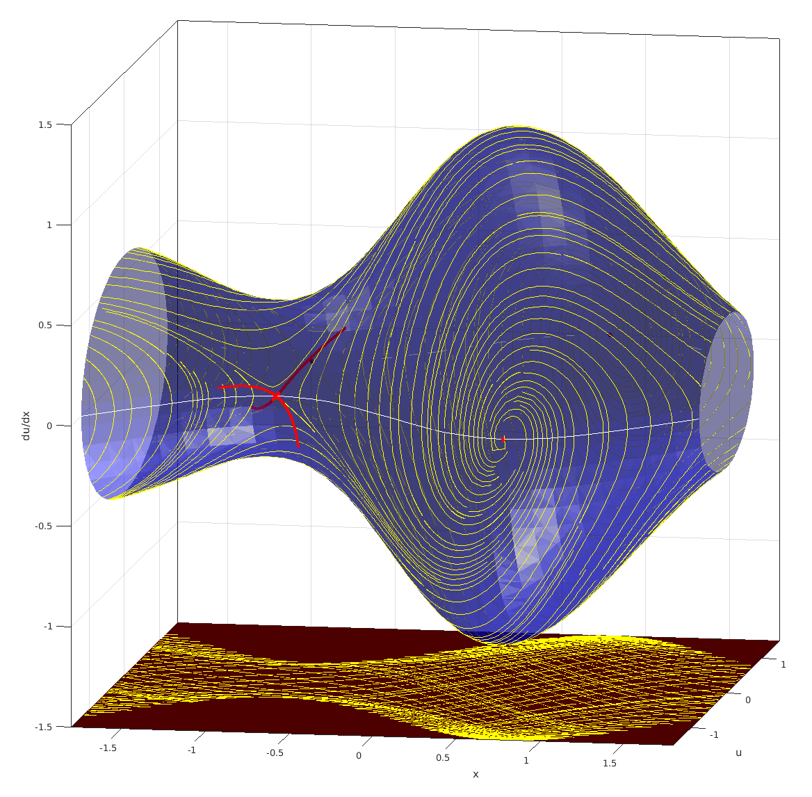
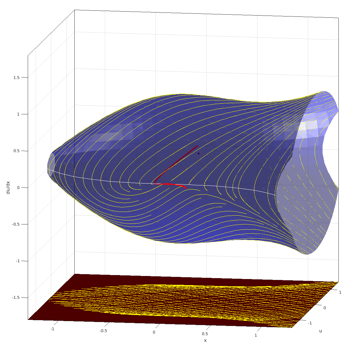
Figure 1. $\mathcal{R}_{1}\subset J_{1}\pi$ given by (5) with generalised and geometric solutions. On the left hand side for the choice $r(t)=1+\sin{(2t)}/2$; on the right hand side for $r(t)=1+t^{3}/3$

Figure 1 shows the surface $\mathcal{R}_{1}$ for two choices of the function $r(t)$. The white line depicts the singularities; irregular ones are marked as red points. The yellow lines on the surface represent generalised solutions computed with the 2.5D version of the algorithm by Jobard and Lefer. At the bottom, one can see the corresponding geometric solutions obtained by a simple projection. Because of their large number, it is not easily visible in the projection that they change direction whenever the generalised solution crosses the white line; but one clearly recognises this behaviour from the form of the generalised solutions.

For a closer analysis of the behaviour at an irregular singularity $\rho=(\bar{t},\pm r(\bar{t}),0)$, one needs the Jacobian of the vector field $X$ at $\rho$. It is easily determined:

$$J=\begin{pmatrix}0&0&(1+\bar{t}^{2})\\ 0&0&0\\ r(\bar{t})\ddot{r}(\bar{t})&0&r(\bar{t})\end{pmatrix}\,.$$

One of its eigenvalues is always $0$ with eigenvector $\left(\begin{smallmatrix}0\\ 1\\ 0\end{smallmatrix}\right)$. However, as this eigenvector is not tangential to $\mathcal{R}_{1}$, we must discard this eigenvalue. If we write $\beta=r(\bar{t})^{2}+4r(\bar{t})\ddot{r}(\bar{t})(1+\bar{t}^{2})$, then the other two – relevant – eigenvalues are given by $(r(\bar{t})\pm\sqrt{\beta})/2$. There arises now a total of five different cases depending on the value of $\beta$. Three of them can be seen in Fig. 1. In the left picture, one can see a saddle point (arising for $\beta>r(\bar{t})^{2}$) and a focus (arising for $\beta<0$). The right picture shows the case of a semi-hyperbolic stationary point with a one-dimensional centre manifold (arising for $\beta=r(\bar{t})^{2}$ which is equivalent to $\ddot{r}(\bar{t})=0$). In this case, further subcases have to be distinguished depending on the values of higher derivatives of $r$ at $\bar{t}$.

Fig. 1 also shows (some of) the invariant manifolds at the irregular singularities. At the saddle point on the left hand side, one can see the stable and the unstable manifold as red lines (the reader may choose which one is the stable manifold, as one could perform the same analysis with the vector field $-X$ for which the eigenvalues just swap signs). As each of these manifolds defines a generalised solution going through the irregular singularity, we conclude that here two generalised solutions intersect. At the focus, no (real) invariant manifolds exist. The generalised solutions approach the irregular singularity asymptotically, however without a well-defined tangent. Hence, here we have no generalised solution through the singularity.

In the right picture, a short piece of (an approximation of) a centre manifold is shown. A closer analysis of the behaviour at this irregular singularity (which is beyond the scope of this article) reveals that we are here actually in a situation where no analytic centre manifold exists (in fact, where the centre manifolds are probably only of finite regularity), i. e. where the Taylor series approximations computed by our algorithm do not converge. This behaviour leads to numerical problems for the algorithm and in such cases one can often determine only experimentally a reasonable order of approximation where the computation succeeds and produces a reasonable result. In our case one can see that the computed approximation probably describes qualitatively correctly the form of the centre manifold but that the piece shown can be accurate only rather close to the singularity, as further away it intersects with other generalised solutions which is not possible. The shown red line approximates one generalised solution going through the irregular singularity. Generally, centre manifolds are not unique and then each centre manifold yields a different generalised solution. It is a classical result that all different centre manifolds are exponentially close to each other and thus possess the same Taylor polynomial (to any order for which it exists). As our algorithm is based on computing a Taylor series approximation, it cannot distinguish different centre manifolds.

6.2. A Quasi-Linear Second-Order Equation

In an optimal control problem related to financial economics, the following scalar quasi-linear second-order equation arises [5]

$$t^{2}\ddot{u}=at\dot{u}+bu-c(\dot{u}-1)^{2}$$ (7)

together with the initial conditions $u(0)=0$ and $\dot{u}(0)=1$. Here $a,b,c\in\mathbbm{R}$ are parameters. To avoid case distinctions, we assume that $bc\neq 0$ and $a+b\neq 0$. Following the above mentioned reduction process for quasi-linear equations, we are lead to study the three-dimensional vector field

$$Y=t^{2}\partial_{t}+t^{2}\dot{u}\partial_{u}+\bigl{(}at\dot{u}+bu-c(\dot{u}-1)^{2}\bigr{)}\partial_{\dot{u}}\,.$$ (8)

Under the above made assumptions on the parameters, the stationary points of this vector field – and thus the impasse points of (7) – lie on the parabola $t=0$ and $bu=c(\dot{u}-1)^{2}$. At the “tip” of the parabola, i. e. at the point $\rho=(0,0,1)$, the Jacobian of $Y$ has $0$ as a triple eigenvalue (and a non-trivial Jordan normal form with two blocks). At all other points on the parabola, the Jacobian has only a double eigenvalue $0$. It is still an open problem to study in detail the local solution behaviour around $\rho$; at the other impasse points a centre manifold reduction yields a planar problem which can be completely analysed.

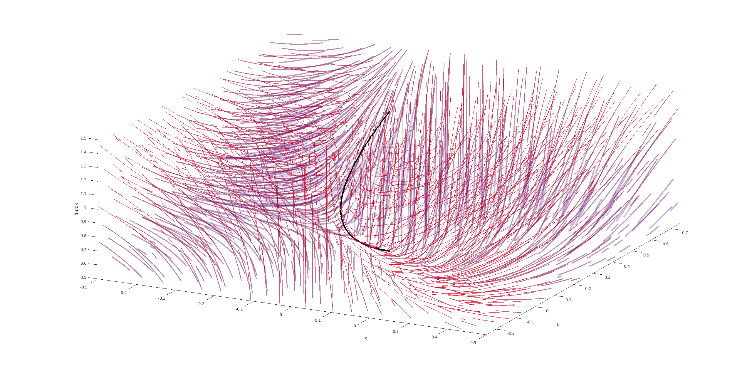
Figure 2. 3D streamlines of the vector field $Y$ given by (8)

Fig. 2 shows a 3D visualisation of the vector field $Y$ given by (8) using the parameter values $a=b=c=1$. The black parabola contains the impasse points. One clearly sees that the extension of the algorithm by Jobard and Lefer to 3D only partly helps with the visualisation. The above mentioned problem that projected streamlines cover each other or intersect is clearly visible and drastically reduces the interpretability of the obtained images. However, one should keep in mind that our goal is to obtain a better understanding of the dynamics in a neighbourhood of the “tip” $\rho$ of the parabola. Here, the real problem is less the 3D visualisation but a mathematical one. If we get too close to the singularity, the numerical integration will break down. As mentioned above, we introduced specifically for this purpose a parameter $d_{\mathrm{s}}$ as stopping criterion for the numerical integration when we approach a singularity. In the example at hand, we could actually get fairly close to the parabola and thus a careful study of the picture reveals at least some indications about the local solution behaviour, in particular if we combine it with the information obtained from the next picture.

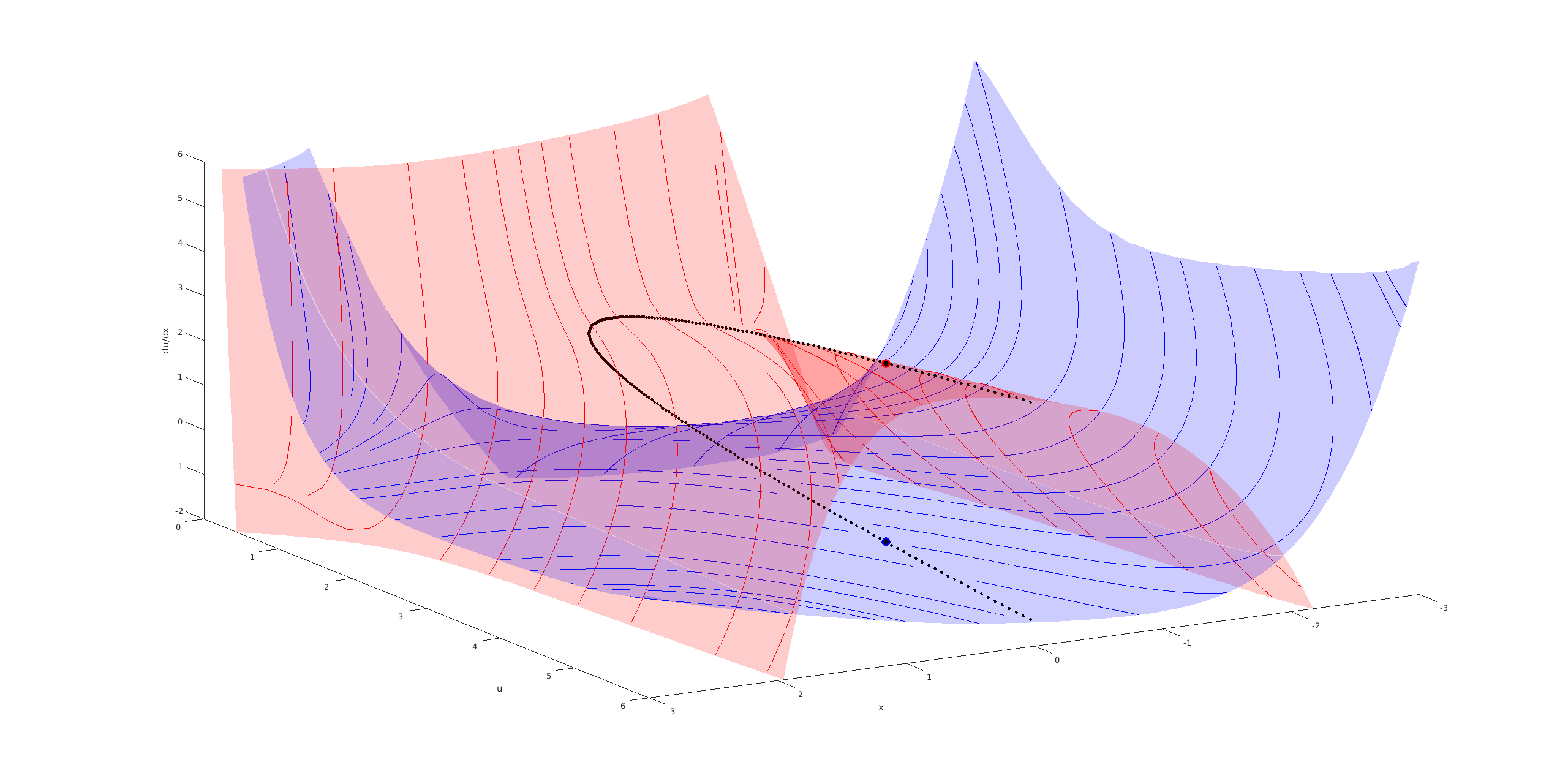
Figure 3. Centre manifolds and reduced dynamics on them for two different impasse points of (7)

Fig. 3 shows approximations of two-dimensional centre manifolds at two points on the parabola away from the “tip” plotted together with the reduced dynamics on them (one point and the corresponding manifold are shown in red, the other one in blue). As the parabola consists entirely of stationary points, it is part of any centre manifold through a point on it which is clearly visible in the picture. Indeed, if one computes the eigenvectors of the Jacobian of $Y$ to the eigenvalue $0$ (away from the “tip” $\rho$ the Jacobian is always diagonalisable), then one of them is tangential to the parabola. The other provides the direction of the reduced dynamics which consists of streamlines cleanly intersecting the parabola.

Fig. 3 was obtained by combining two of the above described algorithms. First, a Taylor series approximation of the centre manifolds and the reduced dynamics on it are computed via the approach of Eirola and von Pfaler. Then, a 2.5D visualisation of the reduced dynamics is determined following the method of Jobard and Lefer. We have plotted rather large parts of the centre manifold approximations and one probably should analyse the quality of the approximation further away from the selected impasse points in more details. The picture seems to indicate that the centre manifolds intersect. While this is surely possible, the 3D picture shown in Fig. 2 gives no indication that such a phenomenon actually occurs.

7. Conclusions

In this article, we briefly sketched the use of geometric techniques, in particular of the Vessiot distribution, for the analysis of implicit ordinary differential equations. We described a suite of Matlab programmes supporting such an analysis with numerical integrations and visualisations. While there is surely still much room for improving the programmes, in particular concerning the 3D visualisation, they already proved useful for the analysis of concrete differential equations.

Our discussion of two concrete examples in Section 6 clearly shows that the analysis of singularities or impasse points cannot be completely automatised even for low-dimensional problems. One needs further (mainly symbolic) computations, firstly to know what pictures could be useful for the analysis and then for a better understanding of what the picture are actually showing. Nevertheless, in our experience pictures like the ones shown in Section 6 are very helpful for unravelling the local solution behaviour around singularities.

References

- [1] V.I. Arnold. Geometrical Methods in the Theory of Ordinary Differential Equations. Grundlehren der mathematischen Wissenschaften 250. Springer-Verlag, New York, edition, 1988.
- [2] T. Bächler, V.P. Gerdt, M. Lange-Hegermann, and D. Robertz. Algorithmic Thomas decomposition of algebraic and differential systems. J. Symb. Comp., 47:1233–1266, 2012.
- [3] W.J. Beyn and W. Kleß. Numerical Taylor expansion of invariant manifolds in large dynamical systems. Numer. Math., 80:1–38, 1998.
- [4] E. Braun. Numerische Analyse und Visualisierung von voll-impliziten gewöhnlichen Differentialgleichungen. Master thesis, Institut für Mathematik, Universität Kassel, 2017.
- [5] P. Brunovský, A. Černý, and M. Winkler. A singular differential equation stemming from an optimal control problem in financial economics. Appl. Math. Opt., 68:255–274, 2013.
- [6] C.K. Chen, S. Yan, H. Yu, N. Max, and K.L. Ma. An illustrative visualization framework for 3D vector fields. Comput. Graph. Forum, 30:1941–1951, 2011.
- [7] F. Dumortier, J. Llibre, and J.C. Artés. Qualitative Theory of Planar Differential Systems. Universitext. Springer-Verlag, Berlin/Heidelberg, 2006.
- [8] T. Eirola and J. von Pfaler. Taylor expansion for invariant manifolds. Numer. Math., 80:1–38, 1998.
- [9] D. Fesser. On Vessiot’s Theory of Partial Differential Equations. PhD thesis, Fachbereich Mathematik, Universität Kassel, 2008.
- [10] D. Fesser and W.M. Seiler. Existence and construction of Vessiot connections. SIGMA, 5:092, 2009.
- [11] B. Jobard and W. Lefer. Creating evenly-spaced streamlines of arbitrary density. In W. Lefer and M. Grave, editors, Visualization in Scientific Computing, Eurographics, pages 43–55. Springer-Verlag, 1997.
- [12] U. Kant and W.M. Seiler. Singularities in the geometric theory of differential equations. In W. Feng, Z. Feng, M. Grasselli, X. Lu, S. Siegmund, and J. Voigt, editors, Dynamical Systems, Differential Equations and Applications (Proc. 8th AIMS Conference, Dresden 2010), volume 2, pages 784–793. AIMS, 2012.
- [13] V.V. Lychagin. Homogeneous geometric structures and homogeneous differential equations. In V.V. Lychagin, editor, The Interplay between Differential Geometry and Differential Equations, Amer. Math. Soc. Transl. 167, pages 143–164. Amer. Math. Soc., Providence, 1995.
- [14] S. Marchesin, C.K. Chen, C. Ho, and K.L. Ma. View-dependent streamlines for 3D vector fields. IEEE Trans. Vis. Comput. Graph., 16:1578–1586, 2010.
- [15] J.F. Pommaret. Systems of Partial Differential Equations and Lie Pseudogroups. Gordon & Breach, London, 1978.
- [16] D.J. Saunders. The Geometry of Jet Bundles. London Mathematical Society Lecture Notes Series 142. Cambridge University Press, Cambridge, 1989.
- [17] W.M. Seiler. Involution — The Formal Theory of Differential Equations and its Applications in Computer Algebra. Algorithms and Computation in Mathematics 24. Springer-Verlag, Berlin, 2010.
- [18] W.M. Seiler. Singularities of implicit differential equations and static bifurcations. In V.P. Gerdt, W. Koepf, E.W. Mayr, and E.V. Vorozhtsov, editors, Computer Algebra in Scientific Computing — CASC 2013, Lecture Notes in Computer Science 8136, pages 355–368. Springer-Verlag, Berlin, 2013.
- [19] W.M. Seiler and M. Seiß. Singular initial value problems for quasi-linear ordinary differential equations. In preparation, 2018.
- [20] W.Y. Sit. An algorithm for solving parametric linear systems. J. Symb. Comp., 13:353–394, 1992.
- [21] J. Tuomela. On singular points of quasilinear differential and differential-algebraic equations. BIT, 37:968–977, 1997.
- [22] J. Tuomela. On the resolution of singularities of ordinary differential equations. Num. Algo., 19:247–259, 1998.
- [23] E. Vessiot. Sur une théorie nouvelle des problèmes généraux d’intégration. Bull. Soc. Math. Fr., 52:336–395, 1924.