Optimal transport: discretization and algorithms

Abstract.

This chapter describes techniques for the numerical resolution of optimal transport problems. We will consider several discretizations of these problems, and we will put a strong focus on the mathematical analysis of the algorithms to solve the discretized problems. We will describe in detail the following discretizations and corresponding algorithms: the assignment problem and Bertsekas auction’s algorithm; the entropic regularization and Sinkhorn-Knopp’s algorithm; semi-discrete optimal transport and Oliker-Prussner or damped Newton’s algorithm, and finally semi-discrete entropic regularization. Our presentation highlights the similarity between these algorithms and their connection with the theory of Kantorovich duality.

1. Introduction

The problem of optimal transport, introduced by Gaspard Monge in 1871 [76], was motivated by military applications. The goal was to find the most economical way to transport a certain amount of sand from a quarry to a construction site. The source and target distributions of sand are seen as probability measures, denoted $\mu$ and $\nu$, and $c(x,y)$ denotes the cost of transporting a grain of sand from the position $x$ to the position $y$, and the goal is to solve the non-convex optimization problem

$$\mathrm{(MP)}=\min_{T_{\#}\mu=\nu}\int c(x,T(x))\mathrm{d}\mu,$$ (1.1)

where $T_{\#}\mu=\nu$ means that $\nu$ is the push-forward of $\mu$ under the transport map $T$. The modern theory of optimal transport has been initiated by Lenoid Kantorovich in the 1940s, via a convex relaxation of Monge’s problem. Given two probability measures $\mu$ and $\nu$, it consists in minimizing

$$\mathrm{(KP)}=\min_{\gamma\in\Gamma(\mu,\nu)}\int c(x,y)\mathrm{d}\gamma(x,y),$$ (1.2)

over the set $\Gamma(\mu,\nu)$ of transport plans between $\mu$ and $\nu$. Kantorovich’s theory has been used and revisited by many authors from the 1980s, allowing a complete solution to Monge’s problem in particular for $c(x,y)=\left\|x-y\right\|^{p}$. Since then, optimal transport has been connected to various domains of mathematics (geometry, probabilities, partial differential equations) but also to more applied domains. Current applications of optimal transport include machine learning [83], computer graphics [87], quantum chemistry [22, 32], fluid dynamics [20, 39, 73], optics [80, 26, 99, 24], economy [49], statistics [27, 30, 61]. The selection of citation above is certainly quite arbitrary, as optimal transport is now more than ever a vivid topic, with more than several hundreds (perhaps even thousands) of articles published every year and containing the words <<optimal transport>>.

There exist many books on the theory of optimal transport, e.g. by Rachev-Rüschendorf [84, 85], by Villani [97, 98] and by Santambrogio [88]. However, there exist fewer books dealing with the numerical aspects, by Galichon [49], by Cuturi-Peyré [83] and one chapter of Santambrogio [88]. The books by Galichon and Cuturi-Peyré are targeted toward applications (in economy and machine learning, respectively) and do not deal in full detail with the mathematical analysis of algorithms for optimal transport. In this chapter, we concentrate on numerical methods for optimal transport relying on Kantorovich duality. Our aim in particular is to provide a self-contained mathematical analysis of several popular algorithms to solve the discretized optimal transport problems.

Kantorovich duality. In the 2000s, the theory of optimal transport was already mature and was used within mathematics, but also in theoretical physics or in economy. However, numerical applications were essentially limited to one-dimensional problems because of the prohibitive cost of existing algorithms for higher dimensional problems, whose complexity was in general more than quadratic in the size of the data. Numerous numerical methods have been introduced since then. Most of them rely the dual problem associated to Kantorovich’s problem (1.2), namely

$$\mathrm{(DP)}=\max_{\varphi\ominus\psi\leqslant c}\int\varphi\mathrm{d}\mu-\int\psi\mathrm{d}\nu,$$ (1.3)

where the maximum is taken over pairs $(\varphi,\psi)$ of functions satisfying $\varphi\ominus\psi\leqslant c$, meaning that $\varphi(x)-\psi(y)\leqslant c(x,y)$ for all $x,y$. Equivalently, the dual problem can be written as the unconstrained maximization problem

$$\mathrm{(DP)}=\max_{\psi}\mathcal{K}(\psi)\ \hbox{ where }\ \mathcal{K}(\psi)=\int\psi^{c}\mathrm{d}\mu-\int\psi\mathrm{d}\nu$$ (1.4)

and $\psi^{c}(x):=\min_{y}c(x,y)+\psi(y)$ is the $c$-transform of $\psi$, a notion closely related to the Legendre-Fenchel transform in convex analysis. The function $\mathcal{K}$ is called the Kantorovitch functional. Kantorovich’s duality theorem asserts that the values of (1.2) and (1.3) (or (1.4)) agree under mild assumptions.

Overview of numerical methods. We now briefly review the most used numerical methods for optimal transport. Note that there is no <<free lunch>> in the sense that there exists no method able to deal efficiently with arbitrary cost function; the computational complexity of most methods depend on the complexity of computing $c$-transforms or smoothed $c$-transforms. In this overview, we skip linear programming methods such as the network simplex, for which we refer to [83].

A. Assignment problem. When the two measures are uniformly supported on two finite sets with cardinal $N$, the optimal transport problem coincides with the assignment problem, described in [21]. The assignment problem can be solved using various techniques, but in this chapter we will concentrate on a dual ascent method called Bertsekas’ auction algorithm [16], whose complexity is also $\mathrm{O}(N^{3})$, but which is very simple to implement and analyze. In §3.2 we note that the complexity can be improved when it is possible to compute discrete $c$-transforms efficiently, namely

$$\psi^{c}(x_{i})=\min_{j}c(x_{i},y_{j})+\psi(y_{j}).$$ (1.5)

B. Entropic regularization. In this approach, one does not solve the original optimal transport problem (1.2) exactly, but instead replaces it with a regularized problem involving the entropy of the transport plan. In the discrete case, it consists in minimizing

$$\min_{\gamma}\sum_{i,j}\gamma_{i,j}c(x_{i},y_{j})+\eta\sum_{i,j}h(\gamma_{i,j}),$$ (1.6)

where $h(r)=r(\log r-1)$ and $\eta>0$ is a small parameter, under the constraints

$$\forall i,~{}\sum_{j}\gamma_{i,j}=\mu_{i},\qquad\forall j,~{}\sum_{i}\gamma_{i,j}=\nu_{j}$$ (1.7)

This idea has been introduced in the field of optimal transport by Galichon and Salanié [50] and by Cuturi [35], see [83, Remark 4.5] for a brief historical account. Adding the entropy of the transport plan makes the problem (1.6) strongly convex and smooth. The dual problem can be solved efficiently using Sinkhorn-Knopp’s algorithm, which involves computing repeatedly the smoothed $c$-transform

$$\psi^{c,\eta}(x_{i})=\eta\log(\mu_{i})-\eta\log\left(\sum_{j}e^{\frac{1}{\eta}(-c(x_{i},y_{j})-\psi(y_{j}))}\right).$$ (1.8)

Sinkhorn-Knopp’s algorithm can be very efficient, provided that the smoothed $c$-transform can be computed efficiently (e.g. in near-linear time).

C. Distance costs. When the cost $c$ satisfies the triangle inequality, the dual problem (1.3) can be further simplified:

$$\max_{\mathrm{Lip}_{c}(\psi)\leqslant 1}\int\psi\mathrm{d}\mu-\int\psi\mathrm{d}\nu,$$ (1.9)

where the maximum is taken over functions satisfying $\left|\psi(x)-\psi(y)\right|\leqslant c(x,y)$ for all $x,y$. The equality between the values of (1.2) and (1.9) is called Kantorovich-Rubinstein’s theorem. This leads to very efficient algorithms when the $1$-Lipschitz constraint can be enforced using only local information, thus reducing the number of constraints. This is possible when the space is discrete and the distance is induced by a graph, or when $c$ is the Euclidean norm or more generally a Riemannian metric. In the latter case, the maximum in (1.9) can be replaced by a supremum over $\mathcal{C}^{1}$ functions $\psi$ satisfying $\left\|\nabla\psi\right\|_{\infty}\leqslant 1$ [94, 9]. Note that the case of distance costs is particularly easy because the $c$-transform of a $1$-Lipschitz function is trivial: $\psi^{c}=-\psi$.

D. Monge-Ampère equation. When the cost is the Euclidean scalar product, $c(x,y)=-\langle x|y\rangle$, the dual problem (1.3) can be reformulated as

$$\max_{\psi}-\int\psi^{*}\mathrm{d}\mu-\int\psi\mathrm{d}\nu,$$ (1.10)

where $\psi^{*}(x)=\max_{y}\langle x|y\rangle-\psi(y)$ is the Legendre-Fenchel transform of $\psi$. If the maximizer $\psi$ is smooth and strongly convex and $\mu$, $\nu$ are probability densities, the optimality condition associated to the dual problem is the Monge-Ampère equation,

$$\begin{cases}\mu(\nabla\psi(y))\det(\mathrm{D}^{2}\psi(y))=\nu(y),\\ \nabla\psi(\mathrm{spt}(\nu))\subseteq\mathrm{spt}(\mu).\end{cases}$$ (1.11)

Note the non-standard boundary conditions appearing on the second line of the equation. The first methods able to deal with these boundary conditions use a “wide-stencil” finite difference discretization [46, 13, 12]. These methods are able to solve optimal transport problems provided that the maximizer of (1.10) is a viscosity solution to the Monge-Ampère equation (1.11), imposing restrictions on its regularity. For the Monge-Ampère equation with Dirichlet conditions, we refer to the recent survey by Neilan, Salgado and Zhang [77].

E. Semi-discrete formulation. The semi-discrete formulation of optimal transport involves a source measure that is a probability density $\mu$ and a target measure $\nu$ which is finitely supported, i.e. $\nu=\sum_{i}\nu_{i}\delta_{y_{i}}$. It was introduced by Cullen in 1984 [34], without reference to optimal transport, and much refined since then [6, 70, 38, 55, 64, 68, 65]. In this setting, the dual problem (1.4) amounts to maximizing the Kantorovitch functional given by

$$\mathcal{K}(\psi)=\int\psi^{c}\mathrm{d}\mu-\int\psi\mathrm{d}\nu=\sum_{i}\int_{\mathrm{Lag}_{y_{i}}(\psi)}c(x,y_{i})+\psi(y_{i})\mathrm{d}\mu(x)-\int\psi\mathrm{d}\nu,$$ (1.12)

where the Laguerre cells are defined by

$$\mathrm{Lag}_{y_{i}}(\psi)=\{x\mid\forall j,c(x,y_{i})+\psi(y_{i})\leqslant c(x,y_{j})+\psi(y_{j})\}.$$ (1.13)

The optimality condition for (1.12) is the following non-linear system of equations,

$$\forall i,\mu(\mathrm{Lag}_{y_{i}}(\psi))=\nu_{i}.$$ (1.14)

In the case $c(x,y)=-\langle x|y\rangle$, this system of equations can see as a weak formulation (in the sense of Alexandrov, see [57, Chapter 1]) of the Monge-Ampère equation (1.11). This “semi-discrete” approach can also be used to solve Monge-Ampère equations with Dirichlet boundary conditions, and has been originally introduced for this purpose [79, 75]. Again, the possibility to solve (1.14) efficiently requires one to be able to compute the Laguerre tessellation (1.13), and thus the $c$-transform, efficiently.

F. Dynamic formulation. This formulation relies on the dynamic formulation of optimal transport, which holds when the cost is $c(x,y)=\left\|x-y\right\|^{2}$ on $\mathbb{R}^{d}$ (or more generally induced by a Riemannian metric), and is known as the Benamou-Brenier formulation:

$$\min_{(\rho,v)}\int_{0}^{1}\int_{\mathbb{R}^{d}}\rho_{t}\left\|v_{t}\right\|^{2}\mathrm{d}x\mathrm{d}t\hbox{\quad with\quad}\begin{cases}\partial_{t}\rho_{t}+\mathrm{div}(\rho_{t}v_{t})=0,\\ \rho_{0}=\mu,\rho_{1}=\nu.\end{cases}$$

Introducing the momentum $m_{t}=\rho_{t}v_{t}$, the problem can be rewritten as

$$\min_{(\rho_{t},m_{t})}\int_{0}^{1}\int_{\mathbb{R}^{d}}\frac{\left\|m_{t}\right\|^{2}}{\rho_{t}}\mathrm{d}x\mathrm{d}t\hbox{\quad with\quad}\begin{cases}\partial_{t}\rho_{t}+\mathrm{div}(m_{t})=0,\\ \rho_{0}=\mu,\rho_{1}=\nu.\end{cases}$$

This optimization problem can be discretized using finite elements [7], finite differences [81] or finite volumes [44], and the discrete problem is then usually solved using a primal-dual augmented Lagrangian method [7] (see also [81, 60]). In practice, the convergence is very costly in terms of number of iterations; note also that each iteration requires the resolution of a $(d+1)$-dimensional Poisson problem to project on the admissible set $\{(\rho,m)\mid\partial_{t}\rho+\mathrm{div}(m)=0\}$. Another possibility is to use divergence-free wavelets [59]. One advantage of the Benamou-Brenier approach is that it is very flexible, easily allowing (Riemannian) cost functions [81], additional quadratic terms [8], penalization of congestion [23], partial transport [69, 31], etc. Finally, the convergence from the discretized problem to the continuous one is subtle and depends on the choice of the discretization, see [67, 28].

In this chapter, we will describe in detail the following discretizations for optimal transport and corresponding algorithms to solve the discretized problems : the assignment problem (A.) through Bertsekas auction’s algorithm, the entropic regularization (B.) through Sinkhorn-Knopp’s algorithm, semi-discrete optimal transport (E.) through Oliker-Prussner or Newton’s methods. These algorithms share a common feature, in that they are all derived from Kantorovich duality. Some of them have been adapted to variants of optimal transport problems, such as multi-marginal optimal transport problems problems [82], barycenters with respect to optimal transport metrics [2], partial [25] and unbalanced optimal transport [31, 66], gradient flows in the Wasserstein space [62, 4], generated Jacobian equations [56, 95]. However, we consider these extensions to be out of the scope of this chapter.

2. Optimal transport theory

This part contains a self-contained introduction to the theory of optimal transport, putting a strong emphasis on Kantorovich Kantorovich duality. Kantorovich duality is at the heart of the most important theorems of optimal transport, such as Brenier and Gangbo-McCann’s theorems on the existence and uniqueness of solution to Monge’s problems and the stability of optimal transport plans and optimal transport maps maps. Kantorovich’s duality is also used in all the numerical methods presented in this chapter.

Background on measure theory.

In the following, we assume that $X$ is a compact metric space, and we denote $\mathcal{C}^{0}(X)$ the space of continuous functions over $X$. We denote $\mathcal{M}(X)$ the space of finite (Radon) measures over $X$, identified with the set of continuous linear forms over $\mathcal{C}^{0}(X)$. Given $\varphi\in\mathcal{C}^{0}(X)$ and $\mu\in\mathcal{M}(X)$, we will often denote $\langle\varphi|\mu\rangle=\int_{X}\varphi\mathrm{d}\mu$. The spaces of non-negative measures and probability measures are defined by

$$\mathcal{M}^{+}(X):=\{\mu\in\mathcal{M}(X)\mid\mu\geqslant 0\},$$

$$\mathcal{P}(X):=\{\mu\in\mathcal{M}^{+}(X)\mid\mu(X)=1\},$$

where $\mu\geqslant 0$ means $\langle\mu|\varphi\rangle\geqslant 0$ for all $\varphi\in\mathcal{C}^{0}(X,\mathbb{R}^{+})$. The three spaces $\mathcal{M}(X)$, $\mathcal{M}^{+}(X)$ and $\mathcal{P}(X)$ are endowed with the weak topology induced by duality with $\mathcal{C}^{0}(X)$, namely $\mu_{n}\to\mu$ weakly if

$$\forall\varphi\in\mathcal{C}^{0}(X),~{}\langle\varphi|\mu_{n}\rangle\xrightarrow{n\to\infty}\langle\varphi|\mu\rangle.$$

A point $x$ belongs to the support of a non-negative measure $\mu$ iff for every $r>0$ one has $\mu(\mathrm{B}(x,r))>0$. The support of $\mu$ is denoted $\mathrm{spt}(\mu)$. We recall that by Banach-Alaoglu theorem, the set of probability measures $\mathcal{P}(X)$ is weakly compact, a fact which will be useful to prove existence and convergence results in optimal transport.

Notation.

Given two functions $\varphi\in\mathcal{C}^{0}(X)$ and $\psi\in\mathcal{C}^{0}(Y)$ we will define $\varphi\oplus\psi\in\mathcal{C}^{0}(X\times Y)$ by $\varphi\oplus\psi(x,y)=\varphi(x)+\psi(y)$. We define $\varphi\ominus\psi$ and $\varphi\otimes\psi$ similarly.

2.1. The problems of Monge and Kantorovich

Monge’s problem

Before introducing Monge’s problem, we recall the definition of push-forward or image measure.

Definition 1 (Push-forward and transport map).

Let $X,Y$ be compact metric spaces, $\mu\in\mathcal{M}(X)$ and $T:X\to Y$ be a measurable map. The push-forward of $\mu$ by $T$ is the measure $T_{\#}\mu$ on $Y$ defined by

$$\forall\varphi\in\mathcal{C}^{0}(Y),\langle\varphi|T_{\#}\mu\rangle:=\langle\varphi\circ T|\mu\rangle,$$

or equivalently if for every Borel subset $B\subseteq Y,~{}~{}\mathrm{T}_{\#}\mu(B)=\mu(T^{-1}(B))$. A measurable map $T:X\to Y$ such that $T_{\#}\mu=\nu$ is also called a transport map between $\mu$ and $\nu$.

Example 1.

If $Y=\{y_{1},\ldots,y_{n}\}$, then $T_{\#}\mu=\sum_{1\leqslant i\leqslant n}\mu(T^{-1}(\{y_{i}\}))\delta_{y_{i}}$.

Example 2.

Assume that $T$ is a $\mathcal{C}^{1}$ diffeomorphism between compact domains $X,Y$ of $\mathbb{R}^{d}$, and assume also that the probability measures $\mu,\nu$ have continuous densities $\rho,\sigma$ with respect to the Lebesgue measure. Then,

$$\int_{Y}\varphi(y)\sigma(y)\mathrm{d}y=\int_{X}\varphi(T(x))\sigma(T(x))\det(\mathrm{D}T(x))\mathrm{d}x.$$

Hence, $T$ is a transport map between $\mu$ and $\nu$ iff

$$\forall\varphi\in\mathcal{C}^{0}(X),\int_{X}\varphi(T(x))\sigma(T(x))\det(\mathrm{D}T(x))\mathrm{d}x=\int_{X}\varphi(T(x))\rho(x)\mathrm{d}x,$$

or equivalently if the (non-linear) Jacobian equation holds

$$\rho(x)=\sigma(T(x))\det(\mathrm{D}T(x)).$$

Definition 2 (Monge’s problem).

Consider two compact metric spaces $X,Y$, two probability measures $\mu\in\mathcal{P}(X)$, $\nu\in\mathcal{P}(Y)$ and a cost function $c\in\mathcal{C}^{0}(X\times Y)$. Monge’s problem is the following optimization problem

$$\mathrm{(MP)}:=\inf\left\{\int_{X}c(x,T(x))\mathrm{d}\mu(x)\mid T:X\to Y\hbox{ and }T_{\#}\mu=\nu\right\}$$ (2.15)

Monge’s problem exhibits several difficulties, one of which is that both the transport constraint ($T_{\#}\mu=\nu$) and the functional are non-convex. Note also that there might exist no transport map between $\mu$ and $\nu$. For instance, if $\mu=\delta_{x}$ for some $x\in X$, then, $\mathrm{T}_{\#}\mu(B)=\mu(T^{-1}(B))=\delta_{T(x)}$. In particular, if $\mathrm{card}(\mathrm{spt}(\nu))>1$, there exists no transport map between $\mu$ and $\nu$.

Kantorovich’s problem

Definition 3 (Marginals).

The marginals of a measure $\gamma$ on a product space $X\times Y$ are the measures $\Pi_{X\#}\gamma$ and $\Pi_{Y\#}\gamma$, where $\Pi_{X}:X\times Y\to X$ and $\Pi_{Y}:X\times Y\to Y$ are their projection maps.

Definition 4 (Transport plan).

A transport plan between two probability measures $\mu,\nu$ on two metric spaces $X$ and $Y$ is a probability measure $\gamma$ on the product space $X\times Y$ whose marginals are $\mu$ and $\nu$. The space of transport plans is denoted $\Gamma(\mu,\nu)$, i.e.

$$\Gamma(\mu,\nu)=\left\{\gamma\in\mathcal{P}(X\times Y)\mid\Pi_{X\#}\gamma=\mu,~{}~{}\Pi_{Y\#}\gamma=\nu\right\}.$$

Note that $\Gamma(\mu,\nu)$ is a convex set.

Example 3 (Product measure).

Note that the set of transport plans $\Gamma(\mu,\nu)$ is never empty, as it contains the measure $\mu\otimes\nu$.

Definition 5 (Kantorovich’s problem).

Consider two compact metric spaces $X,Y$, two probability measures $\mu\in\mathcal{P}(X)$, $\nu\in\mathcal{P}(Y)$ and a cost function $c\in\mathcal{C}^{0}(X\times Y)$. Kantorovich’s problem is the following optimization problem

$$\mathrm{(KP)}:=\inf\left\{\int_{X\times Y}c(x,y)\mathrm{d}\gamma(x,y)\mid\gamma\in\Gamma(\mu,\nu)\right\}$$ (2.16)

Remark 1.

The infimum in Kantorovich’s problem is less than the infimum in Monge’s problem. Indeed, to any transport map $T$ between $\mu$ and $\nu$ one can associate a transport plan, by letting $\gamma_{T}=(\mathrm{id},T)_{\#}\mu$. One can easily check that $\Pi_{X\#}\gamma_{T}=\mu$ and $\Pi_{Y\#}\gamma_{T}=\nu$ so that $\gamma_{T}\in\Gamma(\mu,\nu)$ is a transport plan between $\mu$ and $\nu$. Moreover, by the definition of push-forward,

$$\langle c|\gamma_{T}\rangle=\langle c|(\mathrm{id},T)_{\#}\mu\rangle=\langle c\circ(\mathrm{id},T)|\mu\rangle=\int_{X}c(x,T(x))\mathrm{d}\mu$$

thus showing that $\mathrm{(KP)}\leqslant\mathrm{(MP)}$.

Proposition 1.

Kantorovich’s problem $\mathrm{(KP)}$ admits a minimizer.

Proof.

The definition of $\Pi_{X\#}\gamma=\mu$ can be expanded into

$$\forall\varphi\in\mathcal{C}^{0}(X),\langle\varphi\otimes 1|\gamma\rangle=\langle\varphi|\mu\rangle,$$

from which it is easy to see that the set $\Gamma(\mu,\nu)$ is weakly closed, and therefore weakly compact as a subset of $\mathcal{P}(X\times Y)$, which is weakly compact by Banach-Alaoglu’s theorem. We conclude the existence proof by remarking that the functional that is minimized in $\mathrm{(KP)}$, namely $\mu\mapsto\langle c|\mu\rangle$, is weakly continuous by definition. ∎

2.2. Kantorovich duality

Derivation of the dual problem

The primal Kantorovich problem $\mathrm{(KP)}$ can be reformulated by introducing Lagrange multipliers for the constraints. Namely, we use that for any $\gamma\in\mathcal{M}^{+}(X\times Y)$,

$$\sup_{\varphi\in\mathcal{C}^{0}(X)}-\langle\varphi\otimes 1|\gamma\rangle+\langle\varphi|\mu\rangle=\begin{cases}0&\hbox{ if }\Pi_{X\#}\gamma=\mu\\ +\infty&\hbox{ if not}\end{cases}$$

$$\sup_{\varphi\in\mathcal{C}^{0}(X)}\langle 1\otimes\psi|\gamma\rangle-\langle\psi|\mu\rangle=\begin{cases}0&\hbox{ if }\Pi_{X\#}\gamma=\mu\\ +\infty&\hbox{ if not}\end{cases}$$

to deduce

$$\sup_{\varphi\in\mathcal{C}^{0}(X),\psi\in\mathcal{C}^{0}(Y)}\langle\varphi|\mu\rangle-\langle\psi|\nu\rangle-\langle\varphi\ominus\psi|\gamma\rangle=\begin{cases}0&\hbox{ if }\gamma\in\Gamma(\mu,\nu)\\ +\infty&\hbox{ if not}.\end{cases}$$

This leads to the following formulation of the Kantorovich problem

$$\mathrm{(KP)}=\inf_{\gamma\in\mathcal{M}^{+}(X\times Y)}\sup_{(\varphi,\psi)\in\mathcal{C}^{0}(X)\times\mathcal{C}^{0}(Y)}\langle c-(\varphi\ominus\psi)|\gamma\rangle+\langle\varphi|\mu\rangle-\langle\psi|\nu\rangle$$

Kantorovich dual problem is simply obtained by inverting the infimum and the supremum:

$$\mathrm{(DP)}:=\sup_{\varphi,\psi}\inf_{\gamma\geqslant 0}\langle c-(\varphi\ominus\psi)|\gamma\rangle+\langle\varphi|\mu\rangle-\langle\psi|\nu\rangle.$$

Note that we will often omit the assumptions that $\gamma\in\mathcal{M}(X\times Y)$ and $\varphi,\psi$ are continuous, when the context is clear. The dual problem can further be simplified by remarking that

$$\inf_{\gamma\geqslant 0}\langle c-\varphi\ominus\psi|\gamma\rangle=\begin{cases}0&\hbox{ if }\varphi\ominus\psi\leqslant c\\ -\infty&\hbox{ if not. }\end{cases}$$

Definition 6 (Kantorovich’s dual problem).

Given $\mu\in\mathcal{P}(X)$ and $\nu\in\mathcal{P}(Y)$ with $X,Y$ compact metric spaces and $c\in\mathcal{C}^{0}(X\times Y)$, we define Kantorovich’s dual problem by

$$\mathrm{(DP)}=\sup\left\{\int_{X}\varphi\mathrm{d}\mu-\int_{Y}\psi\mathrm{d}\nu\mid(\varphi,\psi)\in\mathcal{C}^{0}(X)\times\mathcal{C}^{0}(Y),\varphi\ominus\psi\leqslant c\right\}$$ (2.17)

Proposition 2.

Weak duality holds, i.e. $\mathrm{(KP)}\geqslant\mathrm{(DP)}$.

Proof.

Given $(\varphi,\psi,\gamma)\in\mathcal{C}^{0}(X)\times\mathcal{C}^{0}(Y)\times\Gamma(\mu,\nu)$ satisfying the constraint $\varphi\ominus\psi\leqslant c$, one has

$$\langle\varphi|\mu\rangle-\langle\psi|\nu\rangle=\langle\varphi\ominus\psi|\gamma\rangle\leqslant\langle c|\gamma\rangle,$$

where we used $\gamma\in\Gamma(\mu,\nu)$ to get the equality and $\varphi\ominus\psi\leqslant c$ to get the inequality. As a conclusion,

$$\mathrm{(DP)}=\min_{\varphi\ominus\psi\leqslant c}\langle\varphi|\mu\rangle-\langle\psi|\nu\rangle\leqslant\max_{\gamma\in\Gamma(\mu,\nu)}\langle c|\gamma\rangle=\mathrm{(KP)}\qed$$

Existence of solution for the dual problem

Kantorovich’s dual problem $\mathrm{(DP)}$ consists in maximizing a concave (actually linear) functional under linear inequality constraints. It can also also easily be turned into an unconstrained minimization problem. The idea is quite simple: given a certain $\psi\in\mathcal{C}^{0}(Y)$, one wishes to select $\varphi$ on $X$ which is as large as possible (to maximize the term $\langle\varphi|\mu\rangle$ in $\mathrm{(DP)}$) while satisfying the constraint $\varphi\ominus\psi\leqslant c$. This constraint can be rewritten as

$$\forall x\in X,~{}~{}\varphi(x)\leqslant\min_{y\in Y}c(x,y)+\psi(y).$$

The largest function $\varphi$ satisfying it is $\varphi(x)=\min_{y\in Y}c(x,y)+\psi(y)$. Thus,

$$\mathrm{(KP)} =\sup_{\varphi\ominus\psi\leqslant c}\langle\varphi|\mu\rangle-\langle\psi|\nu\rangle$$

$$=\sup_{\psi\in\mathcal{C}^{0}(Y)}\int_{X}\left(\min_{y\in Y}c(x,y)+\psi(y)\right)\mathrm{d}\mu(x)-\int\psi(y)\mathrm{d}\nu(y).$$

This idea is at the basis of many algorithms to solve discrete instances of optimal transport, but also useful in theory. It also suggests to introduce the notion of $c$-transform. .

Definition 7 ($c$-Transform).

The $c$-transform (resp. $\overline{c}$-transform) of a function $\psi:Y\to\mathbb{R}\cup\{+\infty\}$ (resp. $\varphi:X\to\mathbb{R}\cup\{+\infty\}$) is defined as

$$\psi^{c}:x\in X\mapsto\inf_{y\in Y}c(x,y)+\psi(y)$$ (2.18)

$$\varphi^{\overline{c}}:y\in Y\mapsto\sup_{x\in X}-c(x,y)+\varphi(x)$$ (2.19)

Thanks to this notion of $c$-transform, one can reformulate the dual problem $\mathrm{(DP)}$ as an unconstrained maximization problem:

$$\mathrm{(DP)}=\sup_{\psi\in\mathcal{C}^{0}(Y)}\int_{X}\psi^{c}\mathrm{d}\mu-\int_{Y}\psi\mathrm{d}\nu.$$ (2.20)

Remark 2 ($c$-concavity, $\overline{c}$-convexity and $c$-subdifferential).

One can call a function $\varphi$ on $X$ $c$-concave if $\varphi=\psi^{c}$ for some $\psi:Y\to\mathbb{R}\cup\{+\infty\}$ on $Y$. Note that we use the word concave because $\psi^{c}$ is defined through an infimum. Conversely, a function $\psi$ on $Y$ is called $\overline{c}$-convex if $\psi=\varphi^{\overline{c}}$ for some $\varphi:X\to\mathbb{R}\cup\{+\infty\}$. Note the asymetry between the two notions, which is due to the choice of the sign in the constraint in Kantorovich’s problem: in the two equivalent formulations

$$\mathrm{(KP)}=\sup_{\varphi\oplus\psi\leqslant c}\langle\varphi|\mu\rangle+\langle\psi|\nu\rangle=\sup_{\varphi\ominus\psi\leqslant c}\langle\varphi|\mu\rangle-\langle\psi|\nu\rangle,$$

we chose the second one, involving two minus signs. This choice will make it easier to explain some of the algorithms we will present later in the chapter. The $c$-subdifferential of a function $\psi$ on $Y$ is a subset of $X\times Y$ defined by

$$\partial^{c}\psi:=\left\{(x,y)\in X\times Y\mid\psi^{c}(x)-\psi(y)=c(x,y)\right\},\\$$ (2.21)

while the $c$-subdifferential at a point $y$ in $Y$ is given by

$$\partial^{c}\psi(y):=\left\{x\in X,\quad(x,y)\in\partial^{c}\psi\right\}.$$ (2.22)

Remark 3 (Bilinear cost).

When $c(x,y)=-\langle x|y\rangle$, a function is $\overline{c}$-convex if and only if it is convex, and $\varphi^{\overline{c}}$ is the Legendre-Fenchel transform of $-\varphi$.

Proposition 3 (Existence of dual potentials).

$\mathrm{(DP)}$ admits a maximizer, which one can assume to be of the form $(\varphi,\psi)$ such that $\varphi=\psi^{c}$ and $\psi=\varphi^{\overline{c}}$.

The existence of maximizers follows from the fact that a $c$-concave/$\overline{c}$-convex function has the same modulus of continuity as $c$.

(Recall that $\omega:\mathbb{R}^{+}\to\mathbb{R}$ is a modulus of continuity of a function $f:Z\to\mathbb{R}$ on a metric space $(Z,d_{Z})$ if it satisfies $\lim_{t\to 0}\omega(t)=0$ and for every $z,z^{\prime}\in Z$, $\left|f(z)-f(z^{\prime})\right|\leqslant\omega(\mathrm{d}_{Z}(z,z^{\prime}))$.)

Lemma 4 (Properties of $c$-transforms).

Let $\omega:\mathbb{R}^{+}\to\mathbb{R}^{+}$ be a modulus of continuity for $c\in\mathcal{C}^{0}(X\times Y)$ for the distance

$$\mathrm{d}_{X\times Y}((x,y),(x^{\prime},y^{\prime}))=\mathrm{d}_{X}(x,x^{\prime})+\mathrm{d}_{Y}(y,y^{\prime}).$$

Then for every $\varphi\in\mathcal{C}^{0}(X)$ and every $\psi\in\mathcal{C}^{0}(Y)$,

• $\varphi^{\overline{c}}$ and $\psi^{c}$ also admits $\omega$ as modulus of continuity.

• $\psi^{c\overline{c}}\leqslant\psi$ and $\psi^{c\overline{c}c}=\psi^{c}$.

• $\varphi^{\overline{c}c}\geqslant\varphi$ and $\varphi^{\overline{c}c\overline{c}}=\varphi^{\overline{c}}$.

Proof.

Let us first prove the first point. Let $\psi\in\mathcal{C}^{0}(Y)$ and for $x\in X$, let $y_{x}\in Y$ be a point realizing the minimum in the definition of $\psi^{c}$. Then,

$$\psi^{c}(x^{\prime})\leqslant c(x^{\prime},y_{x})+\psi(y_{x})=\psi^{c}(x)+c(x^{\prime},y_{x})-c(x,y_{x})\leqslant\psi^{c}(x)+\omega(\mathrm{d}_{X}(x,x^{\prime})).$$

Exchanging the role of $x$ and $x^{\prime}$ we get $\left|\psi^{c}(x^{\prime})-\psi^{c}(x)\right|\leqslant\omega(\mathrm{d}_{X}(x,x^{\prime}))$ as desired. The proof that $\varphi^{\overline{c}}$ has the $\omega$ as modulus of continuity is similar. We prove now the second point. By definition, one has

$$\psi^{c\overline{c}}(y)=\max_{x\in X}\left(-c(x,y)+\min_{\tilde{y}\in Y}c(x,\tilde{y})+\psi(\tilde{y})\right).$$

By taking $\tilde{y}=y$, one gets $\psi^{c\overline{c}}(y)\leqslant\psi(y)$. Again, by definition, we have

$$\psi^{c\overline{c}c}(x)=\min_{y\in Y}\left(c(x,y)+\max_{\tilde{x}\in X}\left(-c(\tilde{x},y)+\min_{\tilde{y}\in Y}c(\tilde{x},\tilde{y})+\psi(\tilde{y})\right)\right).$$

By taking $\tilde{x}=x$ , one gets $\psi^{c\overline{c}c}(x)\geqslant\psi^{c}(x)$, while taking $\tilde{y}=y$ gives us $\psi^{c\overline{c}c}(x)\leqslant\psi^{c}(x)$. The last point is obtained similarly. ∎

Proof of Proposition 3.

Let $(\varphi_{n},\psi_{n})$ be a maximizing sequence for $\mathrm{(DP)}$, i.e. $\varphi_{n}\ominus\psi_{n}\leqslant c$ and $\lim_{n\to+\infty}\langle\varphi_{n}|\mu\rangle-\langle\psi_{n}|\nu\rangle=\mathrm{(DP)}.$ Define $\hat{\varphi}_{n}=\psi_{n}^{c}$ and $\hat{\psi}_{n}=\hat{\varphi_{n}}^{\overline{c}}$. Then $\hat{\varphi}_{n}\ominus\hat{\psi}_{n}\leqslant c$, $\varphi_{n}\leqslant\hat{\varphi_{n}}$ and $\psi_{n}\geqslant\hat{\psi_{n}}$, which implies

$$\langle\varphi_{n}|\mu\rangle-\langle\psi_{n}|\nu\rangle\leqslant-\langle\psi_{n}|\nu\rangle\leqslant\langle\hat{\varphi}_{n}|\mu\rangle-\langle\hat{\psi}_{n}|\nu\rangle,$$

implying that $(\hat{\varphi}_{n},\hat{\psi}_{n})$ is also a maximizing sequence. Our goal is now to show that this sequence admits a converging subsequence. We first note that we can assume that $\hat{\varphi}_{n}(x_{0})=0$ for all $n$, where $x_{0}$ is a given point in $X$: if this is not the case, we replace $(\hat{\varphi}_{n},\hat{\psi}_{n})$ by $(\hat{\varphi}_{n}-\hat{\varphi}_{n}(x_{0}),\hat{\psi}_{n}+\hat{\varphi}_{n}(x_{0}))$), which is also admissible and has the same dual value. In addition, by Lemma 4, the sequences $(\hat{\varphi}_{n})_{n}$ and $(\hat{\psi}_{n})_{n}$ are equicontinuous. By Arzelà-Ascoli’s theorem, we deduce that they admit subsequences converging respectively to $\varphi\in\mathcal{C}^{0}(x)$ and $\psi\in\mathcal{C}^{0}(Y)$, which are then maximizers for $\mathrm{(DP)}$. ∎

Strong duality and stability of optimal transport plans

We will prove strong duality first in the case where $\mu,\nu$ are finitely supported, and will then use a density argument to deduce the general case. As a byproduct of this theorem, we get a stability result for optimal transport plans (i.e. a limit of optimal transport plans is also optimal).

Theorem 5 (Strong duality).

Let $X,Y$ be compact metric spaces and $c\in\mathcal{C}^{0}(X\times Y)$. Then the maximum is attained in $\mathrm{(DP)}$ and $\mathrm{(KP)}=\mathrm{(DP)}$.

Corollary 6 (Support of OT plans).

Let $\psi$ be a maximizer of (2.20) and $\gamma\in\Gamma(\mu,\nu)$ a transport plan. Then the two assertions are equivalent

• $\gamma$ is an optimal transport plan

• $\mathrm{spt}(\gamma)\subset\partial^{c}\psi:=\{(x,y)\in X\times Y\mid\psi^{c}(x)-\psi(y)=c(x,y)\}$.

As a consequence of Kantorovich duality, we can prove stability of optimal transport plans and optimal transport maps.

Theorem 7 (Stability of OT plans).

Let $X,Y$ be compact metric spaces and let $c\in\mathcal{C}^{0}(X\times Y)$. Consider $(\mu_{k})_{k\in\mathbb{N}}$ and $(\nu_{k})_{k\in\mathbb{N}}$ in $\mathcal{P}(X)$ and $\mathcal{P}(Y)$ converging weakly to $\mu$ and $\nu$ respectively.

• If $\gamma_{k}\in\Gamma(\mu_{k},\nu_{k})$ is optimal then, up to subsequences, $(\gamma_{k})$ converges weakly to an optimal transport plan $\gamma\in\Gamma(\mu,\nu)$.

• Let $(\varphi_{k},\psi_{k})$ be optimal Kantorovich potentials in the dual problem between $\mu_{k}$ and $\nu_{k}$, satisfying $\psi_{k}=\varphi_{k}^{\overline{c}}$ and $\varphi_{k}=\psi_{k}^{c}$. Given a point $x_{0}\in X$, define $\tilde{\psi}_{k}=\psi_{k}-\psi_{k}(x_{0})$ and $\tilde{\varphi}_{k}=\varphi_{k}+\psi_{k}(x_{0})$. Then, up to subsequences, $(\tilde{\psi}_{k},\tilde{\varphi_{k}})$ converges uniformly to $(\varphi,\psi)$ a maximizing pair for $\mathrm{(DP)}$ satisfying $\varphi=\psi^{c}$ and $\psi=\varphi^{\overline{c}}$.

The proof of Theorem 5 relies on a simple reformulation of strong duality – similar to the Karush-Kuhn-Tucker optimality conditions for optimization problems with inequality constraints:

Proposition 8.

Let $\gamma\in\Gamma(\mu,\nu)$ and let $(\varphi,\psi)\in\mathcal{C}^{0}(X)\times\mathcal{C}^{0}(Y)$ such that $\varphi\ominus\psi\leqslant c$. Then, the following statements are equivalent:

• $\varphi\ominus\psi=c$ $\gamma$-a.e.

• $\gamma$ minimizes $\mathrm{(KP)}$, $(\varphi,\psi)$ maximizes $\mathrm{(DP)}$ and $\mathrm{(KP)}=\mathrm{(DP)}$.

Proof.

Assume that $\varphi\ominus\psi=c$ $\gamma$-a.e. Then,

$$\mathrm{(KP)}\leqslant\langle c|\gamma\rangle=\langle\varphi\ominus\psi|\gamma\rangle=\langle\varphi|\mu\rangle-\langle\psi|\nu\rangle\leqslant\mathrm{(DP)}$$

Since in addition $\mathrm{(KP)}\geqslant\mathrm{(DP)}$, all inequalities are equalities, which implies that $\mathrm{(KP)}=\mathrm{(DP)}$, $\gamma$ miminizes $\mathrm{(KP)}$ and $(\varphi,\psi)$ maximizes $\mathrm{(DP)}$. Conversely, if $\mathrm{(KP)}=\mathrm{(DP)}$, $\gamma$ miminizes $\mathrm{(KP)}$ and $(\varphi,\psi)$ maximizes $\mathrm{(DP)}$, then

$$\langle\varphi|\mu\rangle-\langle\psi|\nu\rangle=\mathrm{(DP)}=\mathrm{(KP)}=\langle c|\gamma\rangle\geqslant\langle\varphi\ominus\psi|\gamma\rangle=\langle\varphi|\mu\rangle-\langle\psi|\nu\rangle,$$

implying that $\varphi\ominus\psi=c$ $\gamma$ a.e. ∎

The proof of Theorem 5 also relies on a few elementary lemmas from measure theory.

Lemma 9.

If $\mu_{N}$ converges weakly to $\mu$, then for any point $x\in\mathrm{spt}(\mu)$ there exists a sequence $x_{N}\in\mathrm{spt}(\mu_{N})$ converging to $x$.

Proof.

Consider $x\in\mathrm{spt}(\mu)$. For any $k\in\mathbb{N}$, consider the function $\varphi_{k}(z)=\max(1-kd(x,z),0),$ in $\mathcal{C}^{0}(X)$. Then,

$$\lim_{N\to\infty}\langle\varphi_{k}|\mu_{N}\rangle=\langle\varphi_{k}|\mu\rangle>0,$$

where the last inequality holds because $x$ belongs to the support of $\mu$. Then, there exists $N_{k}$ such that for any $N\geqslant N_{k}$, $\langle\varphi_{k}|\mu_{N}\rangle>0$, implying the existence of $x_{N}\in X$ such that $x_{N}\in\mathrm{spt}(\mu_{N})$ and $d(x_{N},x)\leqslant 1/k$. By a diagonal argument, this allows to construct a sequence of points $(x_{N})_{N\in\mathbb{N}}$ such that $x_{N}\in\mathrm{spt}(\mu_{N})$ and $\lim_{N\to+\infty}x_{N}=x$. ∎

Lemma 10.

Let $X$ be a compact space and $\mu\in\mathcal{P}(X)$. Then, there exists a sequence of finitely supported probability measures weakly converging to $\mu$.

Proof.

For any $\varepsilon>0$, by compactness there exists $N$ points $x_{1},\ldots,x_{N}$ such that $X\subseteq\bigcup_{i}\mathrm{B}(x_{i},\varepsilon)$. We define a partition $K_{1},\ldots,K_{N}$ of $X$ recursively by $K_{i}=\mathrm{B}(x_{i},\varepsilon)\setminus(K_{1}\cup...\cup K_{i-1})$ and we introduce

$$\mu_{\varepsilon}:=\sum_{1\leqslant i\leqslant N}\mu(K_{i})\delta_{x_{i}}.$$

To prove weak convergence of $\mu_{\varepsilon}$ to $\mu$ as $\varepsilon\to 0$, take $\varphi\in\mathcal{C}^{0}(X)$. By compactness of $X$, $\varphi$ admits a modulus of continuity $\omega$, i.e. $\lim_{t\to 0}\omega(t)=0$ and $\left|\varphi(x)-\varphi(y)\right|\leqslant\omega(d(x,y))$. Using that $\operatorname{diam}(K_{i})\leqslant\varepsilon$, we get

$$\left|\int\varphi\mathrm{d}\mu-\int\varphi\mathrm{d}\mu_{\varepsilon}\right|=\left|\sum_{1\leqslant i\leqslant N}\int_{K_{i}}\varphi(x)-\varphi(x_{i})\mathrm{d}\mu\right|\leqslant\omega(\varepsilon),$$

We deduce $\lim_{\varepsilon\to 0}\langle\varphi|\mu_{\varepsilon}\rangle=\langle\varphi|\mu\rangle$, so that $\mu_{\varepsilon}$ weakly converges to $\mu$. ∎

Lemma 11.

If $(\mu,\nu)\in\mathcal{P}(X)\times\mathcal{P}(Y)$ are finitely supported, $\mathrm{(KP)}=\mathrm{(DP)}$.

Proof.

Assume that $\mu=\sum_{1\leqslant i\leqslant N}\mu_{i}\delta_{x_{i}},\nu=\sum_{1\leqslant j\leqslant M}\nu_{j}\delta_{y_{j}},$ where all the $\mu_{i}$ and $\mu_{j}$ are strictly positive, and consider the linear programming problem

$$\mathrm{(KP)}^{\prime}=\min\left\{\sum_{i,j}\gamma_{ij}c(x_{i},y_{j})\mid\gamma_{ij}\geqslant 0,\sum_{j}\gamma_{ij}=\mu_{i},\sum_{i}\gamma_{ij}=\nu_{j}\right\},$$

which admits a solution which we denote $\gamma$. By Karush-Kuhn-Tucker theorem, there exists Lagrange multipliers $(\varphi_{i})_{1\leqslant i\leqslant N},(\psi_{j})_{1\leqslant j\leqslant M}$ and $(\pi_{ij})_{1\leqslant i\leqslant N,1\leqslant j\leqslant M}$ such that

$$\begin{cases}\varphi_{i}-\psi_{j}-c(x_{i},y_{j})=\pi_{ij}\\ \gamma_{ij}\pi_{ij}=0\\ \pi_{ij}\leqslant 0\end{cases}$$

In particular, $\varphi_{i}-\psi_{j}\leqslant c(x_{i},y_{j})$ with equality if $\gamma_{ij}>0$. To prove strong duality between the original problems $\mathrm{(KP)}$ and $\mathrm{(DP)}$, we construct two functions $\hat{\varphi},\hat{\psi}$ such that $\hat{\varphi}\ominus\hat{\psi}\leqslant c$ with equality on the set $\{(x_{i},y_{j})\mid\gamma_{ij}>0\}$. For this purpose, we first introduce

$$\psi(y)=\begin{cases}\psi_{i}&\hbox{ if }y=y_{i}\\ +\infty&\hbox{ if not }\end{cases}$$

and let $\hat{\varphi}=\psi^{c}$, $\hat{\psi}=\hat{\varphi}^{c}$. Let $i\in\{1,\cdots,M\}$. Since $\mu_{i}=\sum_{j}\gamma_{ij}\neq 0$, there exists $j\in\{1,\ldots,M\}$ such that $\gamma_{ij}>0$. Using $\gamma_{ij}\pi_{ij}=0$, we deduce that so that $\varphi_{i}-\psi_{j}=c(x_{i},y_{j})$, giving

$$\hat{\varphi}(x_{i})=\min_{k\in\{1,\ldots,N\}}c(x_{i},y_{k})+\psi_{k}=c(x_{i},y_{j})+\psi_{j}=\varphi_{i}.$$

Similarly, one can show that $\hat{\psi}(y_{j})=\psi_{j}$ for all $j\in\{1,\ldots,M\}$. Finally, define $\gamma=\sum_{ij}\gamma_{ij}\delta_{(x_{i},y_{j})}\in\Gamma(\mu,\nu)$. Then one can check that $\hat{\varphi}\ominus\hat{\psi}\leqslant c$ with equality $\gamma$-a.e., so that $\mathrm{(KP)}=\mathrm{(DP)}$ by Proposition 8. ∎

Proof of Theorem 5.

By Lemma 10, there exists a sequence $\mu_{k}\in\mathcal{P}(X)$ (resp. $\nu_{k}\in\mathcal{P}(Y)$) of finitely supported measures which converge weakly to $\mu$ (resp. $\nu$). We denote $\mathrm{(KP)}_{k}$ and $\mathrm{(DP)}_{k}$ the primal and dual Kantorovich problems between $\mu_{k}$ and $\nu_{k}$. By Proposition 3, there exists a solution $(\varphi_{k},\psi_{k})$ of $\mathrm{(DP)}_{k}$, such that $\varphi_{k}=\psi_{k}^{c}$ and $\psi_{k}=\varphi_{k}^{c}$. Moreover, since strong duality holds for finitely supported measures (Lemma 11), we see (Proposition 8) that $\gamma_{k}$ is supported on the set

$$S_{k}=\{(x,y)\in X\times Y\mid\varphi_{k}(x)-\psi_{k}(y)=c(x,y)\}.$$

Adding a constant if necessary, we can also assume that $\varphi_{k}(x_{0})=0$ for some point $x_{0}\in X$. As $c$-concave functions, $\varphi_{k}$ and $\psi_{k}$ have the same modulus of continuity as the cost function $c$ (see Lemma 4), and they are uniformly bounded (using $\varphi_{k}(x_{0})=0$). Using Arzelà-Ascoli theorem, we can therefore assume that up to subsequences, $(\varphi_{k})$ (resp. $(\psi_{k})$) converges to some $\varphi$ (resp $\psi$) uniformly. Then, one easily sees that $\varphi\ominus\psi\leqslant c$ so that $(\varphi,\psi)$ are admissible for the dual problem $\mathrm{(DP)}$.

By compactness of $\mathcal{P}(X\times Y)$, we can assume that the sequence $\gamma_{k}\in\Gamma(\mu_{k},\nu_{k})$ converges to some $\gamma\in\Gamma(\mu,\nu)$. Moreover, by Lemma 9, every pair $(x,y)\in\mathrm{spt}(\gamma)$ can be approximated by a sequence of pairs $(x_{k},y_{k})\in\mathrm{spt}(\gamma_{k})$ i.e. $\lim_{k\to\infty}(x_{k},y_{k})=(x,y)$. Since $\gamma_{k}$ is supported on $S_{k}$ one has $c(x_{k},y_{k})=\varphi_{k}(x_{k})-\psi_{k}(x_{k})$, which gives at the limit $c(x,y)=\varphi(x)-\psi(y)$. We have just shown that for every point pair $(x,y)$ in $\mathrm{spt}(\gamma)$, $c(x,y)=\varphi(x)-\psi(y)$ where $\varphi,\psi$ is admissible. By Proposition 8, this shows that $\gamma$ and $(\varphi,\psi)$ are optimal for their respective problems and that $\mathrm{(KP)}=\mathrm{(DP)}$. ∎

Corollary 6 is a direct consequence of Proposition 8 and of the strong duality $\mathrm{(KP)}=\mathrm{(DP)}$.

Solution of Monge’s problem for Twisted costs

We now show how to use Kantorovich duality to prove the existence of optimal transport maps when the source measure is absolutely continuous on a compact subset of $\mathbb{R}^{d}$ and when the cost function satisfies the following condition:

Definition 8 (Twisted cost).

Let $\Omega_{X},\Omega_{Y}\subseteq\mathbb{R}^{d}$ be open subsets, and $c\in\mathcal{C}^{1}(\Omega_{X}\times\Omega_{Y})$. The cost function satisfies the twist condition if

$$\forall x_{0}\in\Omega_{X},~{}~{}\hbox{ the map }y\in\Omega_{Y}\mapsto v:=\nabla_{x}c(x_{0},y)\in\mathbb{R}^{d}\hbox{ is injective, }$$ (2.23)

where $\nabla_{x}c(x_{0},y)$ denotes the gradient of $x\mapsto c(\cdot,y)$ at $x=x_{0}$. Given $x_{0}\in\Omega_{X}$ and $v\in\mathbb{R}^{d}$, we denote $y_{c}(x_{0},v)$ the unique point (if it exists) such that $\nabla_{x}c(x_{0},y_{c}(x_{0},v))=v$. The map $v\mapsto y_{c}(x_{0},v)$ is often called the $c$-exponential map at $x_{0}$.

Example 4 (Quadratic cost).

Let $c(x,y)=\left\|x-y\right\|^{2}$. Then, for any $x_{0}\in X$, the map $y\mapsto\nabla_{x}c(x_{0},y)=2(x_{0}-y)$ is injective, so that $c$ satisfies the twist condition. Moreover, given $v\in\mathbb{R}^{d}$, the unique $y$ such that $\nabla_{x}c(x_{0},y)=2(x_{0}-y)=v$ is $y=x_{0}-\frac{1}{2}v$, implying that $y_{c}(x_{0},v)=x_{0}-\frac{1}{2}v$.

The following theorem is due to Brenier [19] in the case of the quadratic cost (i.e. $c(x,y)=\left\|x-y\right\|^{2}$) and Gangbo-McCann in the general case of twisted costs [51].

Given $X\subseteq\Omega_{X}\subset\mathbb{R}^{d}$, we define $\mathcal{P}^{\mathrm{ac}}(X)$ as the set of probability measures on $\Omega_{X}$ that are absolutely continuous with respect to the Lebesgue measure, and with support included in $X$.

Theorem 12 (Brenier [19], Gangbo-McCann [51]).

Let $c\in\mathcal{C}^{1}(\Omega_{X}\times\Omega_{Y})$ be a twisted cost, let $X\subseteq\Omega_{X},Y\subseteq\Omega_{Y}$ be compact sets, and let $(\mu,\nu)\in\mathcal{P}^{\mathrm{ac}}(X)\times\mathcal{P}(Y)$. Then, there exists a $c$-concave function $\varphi\in\mathrm{Lip}(X)$ such that $\nu=T_{\#}\mu$ where $T(x)=y_{c}(x,\nabla\varphi(x))$. Moreover, the only optimal transport plan between $\mu$ and $\nu$ is $\gamma_{T}$.

Example 5.

If $h\in\mathcal{C}^{1}(\mathbb{R}^{d})$ is strictly convex, in particular if $h(x)=\left\|x\right\|^{p}$, then the map $x\mapsto\nabla h(x)$ is injective. Take $c(x,y)=h(x-y)$, so that $y\mapsto\nabla_{x}c(x,y)=\nabla_{x}h(x-y)=\nabla h(x-y)$ is also injective. Moreover, given $x_{0}\in\mathbb{R}^{d}$ and $v\in\mathbb{R}^{d}$, the unique solution $y$ to $v=\nabla h(x_{0}-y)$ is $y=y_{c}(x_{0},v):=x_{0}-(\nabla h)^{-1}(v)$. As a consequence, under the hypothesis of the theorem above, the transport map is of the form

$$T(x)=x-(\nabla h)^{-1}(\nabla\varphi(x))$$

where $\varphi$ is a $c$-convex function.

The following lemma shows that a transport plan is induced by a transport map if it is concentrated on the graph of a map.

Lemma 13.

Let $\gamma\in\Gamma(\mu,\nu)$ and $T:X\to Y$ measurable be such that $\gamma(\{(x,y)\in X\times Y\mid T(x)\neq y\})=0$. Then, $\gamma=\gamma_{T}$.

Proof.

By definition of $\gamma_{T}$ one has $\gamma_{T}(A\times B)=\mu(T^{-1}(B)\cap A)$ for all Borel sets $A\subseteq X$ and $B\subseteq Y$. On the other hand,

$$\gamma(A\times B) =\gamma(\{(x,y)\mid x\in A,\hbox{ and }y\in B\})$$

$$=\gamma(\{(x,y)\mid x\in A,y\in B\hbox{ and }y=T(x)\})$$

$$=\gamma(\{(x,y)\mid x\in A\cap T^{-1}(B),y=T(x)\}$$

$$=\mu(A\cap T^{-1}(B)),$$

thus proving the claim. ∎

Proof of Theorem 12.

Enlarging $X$ if necessary (while keeping it compact and inside $\Omega_{X}$), we may assume that $\mathrm{spt}(\mu)$ is contained in the interior of $X$. First note that by compactness of $X\times Y$ and since $c$ is $\mathcal{C}^{1}$, the cost $c$ is Lipschitz on $X\times Y$. Take $(\varphi,\varphi^{\overline{c}})$ a maximizing pair for $\mathrm{(DP)}$ with $\varphi$ $c$-concave. By the formula $\varphi(x)=\min_{y\in Y}c(x,y)+\varphi^{\overline{c}}(y)$ one can see that $\varphi$ is Lipschitz. By Rademacher theorem, $\varphi$ is differentiable Lebesgue almost everywhere, and by the hypothesis $\mu\in\mathcal{P}^{\mathrm{ac}}(X)$, it is therefore differentiable on a set $B\subseteq\mathrm{spt}(\mu)$ with $\mu(B)=1$. Consider an optimal transport plan $\gamma\in\Gamma(\mu,\nu)$. For every pair of points $(x_{0},y_{0})\in\mathrm{spt}(\gamma)\cap B\times Y$, we have

$$\forall x\in X,\varphi(x)-c(x,y_{0})\leqslant\varphi^{\overline{c}}(y_{0})$$

with equality at $x=x_{0}$, so that $x_{0}$ maximizes the function $\varphi-c(\cdot,y_{0})$. Since $x_{0}\in\mathrm{spt}(\mu)$, $x_{0}$ belongs to the interior of $X$, one necessarily has $\nabla\varphi(x_{0})=\nabla_{x}c(x_{0},y_{0})$. Then, by the twist condition, one necessarily has $y_{0}=y_{c}(x_{0},\nabla\varphi(x_{0}))$. This shows that any optimal transport plan $\gamma$ is supported on the graph of the map $T:x\in B\mapsto y_{c}(x_{0},\nabla\varphi(x_{0}))$, and $\gamma=\gamma_{T}$ by the previous lemma. ∎

We finish this section with a stability result for optimal transport maps (a more general result can be found in [98, Chapter 5]).

Proposition 14 (Stability of OT maps).

Let $X\subseteq\Omega_{X}$ and $Y\subseteq\Omega_{Y}$ be compact subsets of open sets $\Omega_{X},\Omega_{Y}\subseteq\mathbb{R}^{d}$, and $c\in\mathcal{C}^{1}(\Omega_{X}\times\Omega_{Y})$ be a twisted cost. Let $\rho\in\mathcal{P}^{\mathrm{ac}}(X)$, and let $(\mu_{k})\in\mathcal{P}(Y)$ be a sequence of measures converging weakly to $\mu\in\mathcal{P}(Y)$. Define $T_{k}$ (resp. $T$) as the unique optimal transport map between $\rho$ and $\mu_{k}$ (resp. $\rho$ and $\mu$). Then, $\lim_{k\to+\infty}\left\|T_{k}-T\right\|_{\mathrm{L}^{1}(\rho)}=0$.

Remark 4.

Note that unlike the stability theorem for optimal transport plans (Theorem 7), the convergence in Proposition 14 is for the whole sequence and not up to subsequence. This theorem is not quantitative, and there exists very few quantitative variants of this theorem. We are aware of two such results. To state them, given a fixed $\rho\in\mathcal{P}(X)$ and $\mu\in\mathcal{P}(Y)$, we denote $T_{\mu}$ the unique optimal transport map between $\rho$ and $\mu$.

• A first result of Ambrosio, reported in an article of Gigli [53, Proposition 3.3 and Corollary 3.4], shows that if $\mu_{0}$ is such that the optimal transport map $T_{\mu_{0}}$ is Lipschitz, then

  $$\left\|T_{\mu}-T_{\mu_{0}}\right\|_{\mathrm{L}^{2}(\rho)}^{2}\leqslant C(\mu_{0})\operatorname{W}_{2}(\mu,\mu_{0}).$$

  The theorem in [53] holds for the quadratic cost on $\mathbb{R}^{d}$. It was recently generalized to other cost functions [5].

• Berman [15] proves a global estimate, not assuming the regularity of $T_{\mu_{0}}$ but with a worse Hölder exponent, of the form

  $$\left\|T_{\mu}-T_{\mu_{0}}\right\|_{\mathrm{L}^{2}(\rho)}^{2}\leqslant C\operatorname{W}_{1}(\mu,\mu_{0})^{1/2^{d-1}},$$

  assuming that $\rho$ is bounded from below on a compact convex domain of $\mathbb{R}^{d}$, when the cost is quadratic. The constant then $C$ only depends on $X,Y$ and $\rho$. Recently a similar bound with an exponent independent on the dimension was obtained by Mérigot, Delalande and Chazal [71]:

  $$\left\|T_{\mu}-T_{\mu_{0}}\right\|_{\mathrm{L}^{2}(\rho)}^{2}\leqslant C\operatorname{W}_{1}(\mu,\mu_{0})^{1/15}.$$

Proof.

As before, without loss of generality, we assume that $\mathrm{spt}(\sigma)$ lies in the interior of $X$. Let $(\varphi_{k},\psi_{k})$ be solutions to $\mathrm{(DP)}_{k}$, which are $c$-conjugate to each other, and such that $\varphi_{k}(x_{0})=0$ for some $x_{0}\in X$. Then, by stability of Kantorovich potentials, there exists a subsequence $(\varphi_{k},\psi_{k})$ (which we do not relabel) which converges uniformly to $(\varphi,\psi)$. Moreover, $(\varphi,\psi)$ are Kantorovich potentials for $\mathrm{(DP)}$, and are also $c$-conjugate to each other.

Since $\varphi,\varphi_{k}\in\mathrm{Lip}(X)$ are differentiable almost everywhere, there exists a subset $Z\subseteq\mathrm{spt}(\sigma)$ with $\mu(Z)=1$ and such that for all $x\in Z$, $\nabla\varphi_{k}$ exists for all $k$ and $\nabla\varphi$ exists. Let $x\in Z$. Using

$$\varphi_{k}(x)-\psi_{k}(T_{k}(x))=c(x,T_{k}(x)),$$

we get that for any cluster point $y$ of the sequence $(T_{k}(x))_{k}$,

$$\begin{cases}\varphi(x)-\psi(y)=c(x,y),\\ \varphi(x^{\prime})-\psi(y)\leqslant c(x^{\prime},y)&\forall x^{\prime}\in X\end{cases},$$

where the second inequality is obtained using $\varphi_{k}\ominus\psi_{k}\leqslant c$. Thus, as in the proof of Brenier-McCann-Gangbo’s theorem, $x$ is a minimizer of $c(\cdot,y)-\varphi$, i.e. $\nabla_{x}c(x,y)=\nabla\varphi(x)$, implying that $y=y_{c}(x,\nabla\varphi(x))=T(x)$. By compactness, this shows that the whole sequence $(T_{k}(x))_{k}$ converges to $S(x)$. Therefore, $T_{k}$ converges $\sigma$-almost everywhere to $T$, and $\mathrm{L}^{1}(\sigma)$ convergence follows easily. ∎

2.3. Kantorovich’s functional

As already mentioned in Equation (2.20), the Kantorovich’s dual problem $\mathrm{(DP)}$ can be expressed as an unconstrained maximization problem:

$$\mathrm{(DP)}=\max_{\psi\in\mathcal{C}^{0}(Y)}\int_{X}\psi^{c}\mathrm{d}\mu-\int_{Y}\psi\mathrm{d}\nu.$$

This motivates the definition of Kantorovich’s functional as follows

Definition 9.

The Kantorovitch functional is defined on $\mathcal{C}^{0}(Y)$ by

$$\mathcal{K}(\psi)=\int_{X}\psi^{c}\mathrm{d}\mu-\int_{Y}\psi\mathrm{d}\nu.$$ (2.24)

The Kantorovitch dual problem therefore amounts to maximizing the Kantorovitch functional:

$$\mathrm{(DP)}=\max_{\psi\in\mathcal{C}^{0}(Y)}\mathcal{K}(\psi).$$

This subsection is devoted to the general computation of the superdifferential of Kantorovich’s functional when $Y$ is finite. This computation will be used to construct and study algorithms for discretized optimal transport problems. The definition, as well as basic properties on the superdifferential $\partial^{+}F$ of a function $F$ are recalled in Appendix 5.1.

Proposition 15.

Let $X$ be a compact space, $Y$ be finite, $c\in\mathcal{C}^{0}(X\times Y)$ and $\mu\in\mathcal{P}(X)$ and $\nu\in\mathcal{P}(Y)$. Then, for all $\psi_{0}\in\mathbb{R}^{Y}$,

$$\partial^{+}\mathcal{K}(\psi_{0})=\{\Pi_{Y\#}\gamma-\nu\mid\gamma\in\Gamma_{\psi_{0}}(\mu)\}.$$ (2.25)

where $\Gamma_{\psi_{0}}(\mu)$ is the set of probability measures on $X\times Y$ with first marginal $\mu$ and supported on the $c$-subdifferential $\partial^{c}\psi_{0}$ (defined in Eq. (2.21)), i.e.

$$\Gamma_{\psi_{0}}(\mu)=\{\gamma\in\mathcal{P}(X\times Y)\mid\Pi_{X\#}\gamma=\mu\hbox{ and }\mathrm{spt}(\gamma)\subseteq\partial^{c}\psi_{0}\}.$$ (2.26)

Proof.

Let $\gamma\in\Gamma_{\psi_{0}}(\mu)$. Then, for all $\psi\in\mathbb{R}^{Y}$,

$$\mathcal{K}(\psi) =\int\psi^{c}\mathrm{d}\mu-\int\psi\mathrm{d}\nu$$

$$=\int\psi^{c}(x)\mathrm{d}\gamma(x,y)-\int\psi\mathrm{d}\nu$$

$$\leqslant\int c(x,y)+\psi(y)\mathrm{d}\gamma(x,y)-\int\psi\mathrm{d}\nu,$$

where we used $\Pi_{X\#}\gamma=\mu$ to get the second equality and $\psi^{c}(x)\leqslant c(x,y)+\psi(y)$ to get the inequality. Note also that equality holds if $\psi=\psi_{0}$, by assumption on the support of $\gamma$. Hence,

$$\mathcal{K}(\psi) \leqslant\mathcal{K}(\psi_{0})+\int(\psi(y)-\psi_{0}(y))\mathrm{d}\gamma(x,y)-\int(\psi-\psi_{0})\mathrm{d}\nu$$

$$=\mathcal{K}(\psi_{0})+\langle\Pi_{Y\#}\gamma-\nu|\psi-\psi_{0}\rangle.$$

This implies by definition that $\Pi_{Y\#}\gamma-\nu$ lies in the superdifferential $\partial^{+}\mathcal{K}(\psi_{0})$, giving us the inclusion

$$D(\psi_{0}):=\{\Pi_{Y\#}\gamma-\nu\mid\gamma\in\Gamma_{\psi_{0}}(\mu)\}\subseteq\partial^{+}\mathcal{K}(\psi_{0}).$$

Note also that the superdifferential of $\mathcal{K}$ is non-empty at any $\psi_{0}\in\mathbb{R}^{Y}$, so that $\mathcal{K}$ is concave. As a concave function on the finite-dimensional space $\mathbb{R}^{Y}$, $\mathcal{K}$ is differentiable almost everywhere and one has $\partial\mathcal{K}^{+}(\psi)=\{\nabla\mathcal{K}(\psi)\}$ at differentiability points.

We now show that $\partial\mathcal{K}^{+}(\psi_{0})\subset D(\psi_{0})$, using the characterization of the subdifferential recalled in the Appendix:

$$\partial\mathcal{K}^{+}(\psi_{0})=\operatorname{conv}\left\{\lim_{n\to\infty}\nabla\mathcal{K}(\psi^{n})\mid(\psi^{n})_{n\in\mathbb{N}}\in S\right\},$$

where $S$ is the set of sequences $(\psi^{n})_{n\in\mathbb{N}}$ that converge to $\psi_{0}$, such that $\nabla\mathcal{K}(\psi^{n})$ exist and admit a limit as $n\to+\infty$. Let $v=\lim_{n\to\infty}\nabla\mathcal{K}(\psi^{n})$ , where $(\psi^{n})_{n\in\mathbb{N}}$ belongs to the set $S$. For every $n$, there exists $\gamma^{n}\in\Gamma_{\psi^{n}}(\mu)$ such that $\nabla\mathcal{K}(\psi^{n})=v^{n}:=\Pi_{Y\#}\gamma^{n}-\nu$. By compactness of $\mathcal{P}(X\times Y)$, one can assume (taking a subsequence if necessary) that $\gamma^{n}$ weakly converges to some $\gamma$, and it is not difficult to check that $\gamma\in\Gamma_{\psi_{0}}(\mu),$ ensuring that the sequence $v^{n}$ converges to some $v\in D(\psi_{0})$. Thus,

$$\left\{\lim_{n\to\infty}\nabla\mathcal{K}(\psi^{n})\mid(\psi^{n})_{n\in\mathbb{N}}\in S\right\}\subseteq D(\psi_{0}).$$

Taking the convex hull and using the convexity of $D(\psi_{0})$, we get $\partial^{+}\mathcal{K}(\psi_{0})\subseteq D(\psi_{0})$ as desired. ∎

As a corollary of this proposition, we obtain an explicit expression for the left and right partial deriatives of $\mathcal{K}$, and a characterization of its differentiability. In this corollary, we use the terminology of semi-discrete optimal transport (Section 4.1), and we will refer to the $c$-subdifferential at $y\in Y$ as Laguerre cell associated to $y$ and we will denote it by $\mathrm{Lag}_{y}(\psi)$.

$$\mathrm{Lag}_{y}(\psi):=\{x\in X\mid\forall z\in Y,c(x,y)+\psi(y)\leqslant c(x,z)+\psi(z)\}.$$ (2.27)

We also need to introduce the strict Laguerre cell $\mathrm{SLag}_{y}(\psi)$:

$$\mathrm{SLag}_{y}(\psi):=\{x\in X\mid\forall z\in Y,c(x,y)+\psi(y)<c(x,z)+\psi(z)\}.$$ (2.28)

Corollary 16 (Directional derivatives of $\mathcal{K}$).

Let $\psi\in\mathbb{R}^{Y}$, $y\in Y$ and define $\kappa(t)=\mathcal{K}(\psi^{t})$ where $\psi^{t}=\psi+t\mathbf{1}_{y}$. Then, $\kappa$ is concave and

$$\partial^{+}\kappa(t)=[\mu(\mathrm{SLag}_{y}(\psi^{t}))-\nu(\{y\}),\mu(\mathrm{Lag}_{y}(\psi^{t}))-\nu(\{y\})]$$

In particular $\mathcal{K}$ is differentiable at $\psi\in\mathbb{R}^{Y}$ iff $\mu(\mathrm{Lag}_{y}(\psi)\setminus\mathrm{SLag}_{y}(\psi))=0$ for all $y\in Y$, and in this case

$$\nabla\mathcal{K}(\psi)=\Big{(}\mu(\mathrm{Lag}_{y}(\psi))-\nu(\{y\})\Big{)}_{y\in Y}.$$

Proof.

Using Hahn-Banach’s extension theorem, one can easily see that the super-differential of $\kappa$ at $t$ is the projection of the super-differential $\mathcal{K}$ at $\psi^{t}$:

$$\partial^{+}\kappa(t)=\left\{\langle\pi|\mathbf{1}_{y}\rangle\mid\pi\in\partial^{+}\mathcal{K}(\psi^{t})\right\}.$$

Combining with the previous proposition we get

$$\partial^{+}\kappa(t) =\left\{\langle\Pi_{X\#\gamma}-\nu|\mathbf{1}_{y}\rangle\mid\gamma\in\Gamma_{\psi^{t}}(\mu)\right\}$$

$$=\left\{\gamma(X\times\{y\})-\nu(\{y\})\mid\gamma\in\Gamma_{\psi^{t}}(\mu)\right\}$$

To obtain the desired formula for $\partial\kappa^{+}(t)$, it remains to prove that

$$\max\left\{\gamma(X\times\{y\})\mid\gamma\in\Gamma_{\psi^{t}}(\mu)\right\}=\mu(\mathrm{Lag}_{y}(\psi^{t})),$$

$$\min\left\{\gamma(X\times\{y\})\mid\gamma\in\Gamma_{\psi^{t}}(\mu)\right\}=\mu(\mathrm{SLag}_{y}(\psi^{t})).$$

We only prove the first equality, the second one being similar. Denote $Z=X\setminus\mathrm{Lag}_{y}(\psi^{t})$, so that for any $\gamma\in\Gamma_{\psi^{t}}(\mu)$,

$$\gamma(X\times\{y\})=\gamma(\mathrm{Lag}_{y}(\psi^{t})\times\{y\})+\gamma(Z\times\{y\}).$$

Moreover, by definition of $\mathrm{Lag}_{y}(\psi^{t})$, $Z\times\{y\}\cap\partial^{c}\psi^{t}=\emptyset$. Since $\gamma$ belongs to $\Gamma_{\psi^{t}}(\mu)$, we have $\mathrm{spt}(\gamma)\subseteq\partial^{c}\psi^{t}$ so that $\gamma(Z\times\{y\})=0$. This gives us

$$\gamma(X\times\{y\})=\gamma(\mathrm{Lag}_{y}(\psi^{t})\times\{y\})\leqslant\gamma(\mathrm{Lag}_{y}(\psi^{t})\times Y)=\mu(\mathrm{Lag}_{y}(\psi^{t})),$$

where we used $\Pi_{X\#}\gamma=\mu$ to get the last equality. This proves that

$$\sup\left\{\gamma(X\times\{y\})\mid\gamma\in\Gamma_{\psi^{t}}(\mu)\right\}\leqslant\mu(\mathrm{Lag}_{y}(\psi^{t})).$$

To show equality, we consider an explicit $\gamma\in\Gamma_{\psi^{t}}(\mu)$ using a map $T:X\to Y$ defined as follows: for $x\in\mathrm{Lag}_{y}(\psi^{t})$, we set $T(x)=y$ and for points $x\not\in\mathrm{Lag}_{y}(\psi^{t})$, we define $T(x)$ to be an arbitrary $z\in Y$ such that $x\in\mathrm{Lag}_{z}(\psi^{t})$. Then, one can readily check that $\gamma=(\mathrm{id},T)_{\#}\mu$ belongs to $\Gamma_{\psi^{t}}(\mu)$ and that by construction, $\gamma(X\times\{y\})=\mu(\mathrm{Lag}_{y}(\psi^{t}))$. ∎

3. Discrete optimal transport

In this part we present two algorithms for solving discrete optimal transport problems, wich can be both be interpreted using Kantorovich’s duality:

• The first one is Bertsekas’ auction algorithm, which allows to solve optimal transport problem where the source and targed measures are uniform over two sets with the same cardinality, a case known as the assignment problem in combinatorial optimization. Bertsekas’ algorithm is a coordinate-ascent method that iteratively modifies the coordinates of the dual variable $\psi$ so as to reach a maximizer of the Kantorovitch functional $\mathcal{K}(\psi)$.

• The second algorithm is the Sinkhorn-Knopp’s algorithm that allows to solve the entropic regularization of (discrete) optimal transport problems. This algorithm can be seen as a block-coordinate ascent method since it amounts to maximizing the dual of the regularized optimal transport problem, denoted by $\mathcal{K}^{\eta}(\varphi,\psi)$, by alternatively optimizing with respect to the two dual variables $\varphi$ and $\psi$.

3.1. Formulation of discrete optimal transport

Primal and dual problems

We consider in this section that the two sets $X$ and $Y$ are finite, and we consider two discrete probability measures $\mu=\sum_{x\in X}\mu_{x}\delta_{x}$ and $\nu=\sum_{y\in Y}\nu_{y}\delta_{y}$. This setting occurs frequently in applications. The set of transport plans is then given by

$$\Gamma(\mu,\nu)=\left\{\gamma=\sum_{x,y}\gamma_{x,y}\delta_{(x,y)}\mid\ \gamma_{x,y}\geqslant 0,\ \sum_{y\in Y}\gamma_{x,y}=\mu_{x},\ \sum_{x\in X}\gamma_{x,y}=\nu_{y}\right\},$$

and is often referred to as the transportation polytope. In this discrete setting, we will conflate a transport plan $\gamma\in\Gamma(\mu,\nu)$ with the matrix $(\gamma_{x,y})_{(x,y)\in X\times Y}$, which formally is the density of $\gamma$ with respect to the counting measure. The constraint $\sum_{y}\gamma_{x,y}=\mu_{x}$ encodes the fact that all mass from $x$ is transported somewhere in $Y$, while the constraint $\sum_{x}\gamma_{x,y}=\nu_{y}$ tells us that the mass at $y$ is transported from somewhere in $X$. The Kantorovitch problem for a cost function $c:X\times Y\to\mathbb{R}$ then reads

$$\mathrm{(KP)}=\min_{\gamma\in\Gamma(\mu,\nu)}\sum_{x\in X,y\in Y}c(x,y)\gamma_{x,y}.$$ (3.29)

As seen in Section 2.2, the dual $\mathrm{(DP)}$ of this linear programming problem amounts to maximizing the Kantorovitch functional $\mathcal{K}$ (2.24), which in this setting can be expressed as

$$\mathcal{K}(\psi)=\sum_{x\in X}\min_{y\in Y}(c(x,y)+\psi(y))\mu_{x}-\sum_{y\in Y}\psi(y)\nu_{y},$$ (3.30)

where $\psi\in\mathbb{R}^{Y}$ is a function over the finite set $Y$. Since strong duality holds (Theorem 5), one has

$$\mathrm{(KP)}=\mathrm{(DP)}=\max_{\psi\in\mathbb{R}^{Y}}\mathcal{K}(\psi).$$

Remark 5.

Knowing a maximizer $\psi\in\mathbb{R}^{Y}$ of $\mathcal{K}$ does not directly allow to recover an optimal transport plan $\gamma$. However, by Corollary 6, we know that any transport plan $\gamma\in\Gamma(\mu,\nu)$ is optimal if and only if its support is included in the $c$-subdifferential of $\psi$:

$$\mathrm{spt}(\gamma)\subset\partial^{c}\psi=\Big{\{}(x,y)\in X\times Y\mid\psi^{c}(x)=c(x,y)+\psi(y)\Big{\}}.$$

3.2. Linear assignment via coordinate ascent

Assignment problem

When the two sets $X$ and $Y$ have the same cardinal $N$ and when $\mu$ and $\nu$ are uniform probability measures over these sets, namely

$$\mu=\frac{1}{N}\sum_{x\in X}\delta_{x},\quad\nu=\frac{1}{N}\sum_{y\in Y}\delta_{y},$$ (3.31)

then Monge’s problem corresponds to the (linear) assignment problem $\mathrm{(AP)}$ which is one of the most famous combinatorial optimization problem:

$$\mathrm{(AP)}=\min\left\{\frac{1}{N}\sum_{x\in X}c(x,\sigma(x))\mid\sigma:X\to Y\mbox{ is a bijection }\right\}.$$ (3.32)

This problem and its variants have generated a very important amount of research, as demonstrated by the bibliography of the book by Burkard, Dell’Amico and Martello on this topic [21].

Note that the set of bijections from $X$ to $Y$ has cardinal $N!$, making it practically impossible to solve $\mathrm{(AP)}$ through direct enumeration. Using Birkhoff’s theorem on bistochastic matrices, we will show that the assignment problem coincides with the Kantorovitch problem.

Definition 10 (Bistochastic matrices).

A $N$-by-$N$ bistochastic matrix is a square matrix $M\in\mathcal{M}_{N}(\mathbb{R})$ with non-negative coefficients such that the sum of any row and any column equals one:

$$\forall i\in\{1,\ldots,N\},\sum_{j}M_{ij}=1,\quad\forall j\in\{1,\ldots,N\},\sum_{i}M_{ij}=1$$

We denote the set of $N$-by-$N$ bistochatic matrices as $\mathcal{B}_{N}\subseteq\mathcal{M}_{N}(\mathbb{R})$.

Definition 11 (Permutation matrix).

The set of permutations (bijections) from $\{1,\ldots,N\}$ to itself is denoted $\mathfrak{S}_{N}$. Given a permutation $\sigma\in\mathfrak{S}_{N},$ we associate the permutation matrix

$$M[\sigma]_{ij}=\begin{cases}1\hbox{ if }\sigma(i)=j\\ 0\hbox{ if not}\end{cases}.$$

One can easily check that if $\sigma$ is a permutation, then $M[\sigma]$ belongs to $\mathcal{B}_{N}$. Birkhoff’s theorem on the other hand asserts that the extremal points of the polyhedron $\mathcal{B}_{N}$ are permutation matrices, implying thanks to Krein-Milman theorem that every bistochastic matrix can be obtained as a (finite) convex combination of permutation matrices.

Theorem 17 (Birkhoff).

The extremal points of $\mathcal{B}_{N}$ are the permutation matrices. In particular, $\mathcal{B}_{N}=\operatorname{conv}\{M[\sigma]\mid\sigma\in\mathfrak{S}_{N}\}$.

Kantorovitch’s problem $\mathrm{(KP)}$ amounts to minimizing a linear function over the set of bistochastic matrices which is convex. Birkoff’s theorem implies that there exists a bijection that solves this problem $\mathrm{(KP)}$, hence the following theorem:

Theorem 18.

Let $\mu$ and $\nu$ be as in (3.31). Then, $\mathrm{(AP)}=\mathrm{(KP)}$.

Proof.

Take an arbitrary ordering of the points in $X$ and $Y$, i.e. $X=\{x_{1},\ldots,x_{N}\}$ and $Y=\{y_{1},\ldots,y_{N}\}$. Then $\gamma\in\mathbb{R}^{X\times Y}\simeq\mathcal{M}_{N}(\mathbb{R})$ is a transport plan between $\mu$ and $\nu$ iff $N\gamma\in\mathcal{B}_{N}$. Since bistochastic matrices include permutation matrices, we have $\mathrm{(KP)}\leqslant\mathrm{(AP)}$, and the converse follows from the fact that the minimum in $\mathrm{(KP)}$ is attained at an extreme point of $\mathcal{B}_{N}$, i.e. a permutation matrix. ∎

Dual coordinate ascent methods

We follow Bertsekas [16] by trying to solve the assignment problem $\mathrm{(AP)}$ through the unconstrained dual problem (3.1). Combining Theorem 18 and Corollary 6, we have the following proposition.

Proposition 19.

The following statements are equivalent

• $\psi$ is a global maximizer of the Kantorovitch functional $\mathcal{K}$

• There exists a bijection $\sigma:X\to Y$ that satisfies

  $$\forall x\in X,~{}c(x,\sigma(x))+\psi(\sigma(x))=\min_{y\in Y}c(x,y)+\psi(y).$$

A bijection $\sigma$ satisfying this last equation is a solution to the linear assignment problem.

The idea of Bertsekas [16] is to iteratively modify the weights $\psi\in\mathbb{R}^{Y}$ so as to reach a maximizer of $\mathcal{K}$. By Corollary 16, the gradient of the Kantorovitch functional, when it exists, is given by

$$\nabla\mathcal{K}(\psi)=\frac{1}{N}\Big{(}\mathrm{card}(\mathrm{Lag}_{y}(\psi))-1\Big{)}_{y\in Y}.$$

In addition, recalling the definition of a Laguerre cell,

$$\mathrm{Lag}_{y}(\psi)=\{x\in X\mid\forall y^{\prime}\in Y,~{}c(x,y)+\psi(y)\leqslant c(x,y^{\prime})+\psi(y^{\prime})\},$$

one can see that $\mathrm{card}(\mathrm{Lag}_{y}(\psi))$ is obviously decreasing when $\psi(y)$ increases. Therefore, in order to maximize the concave function $\mathcal{K}$, it is natural to increase the weight $\psi(y)$ of any Laguerre cells that satisfy $\mathrm{card}(\mathrm{Lag}_{y}(\psi))>1$. In the following lemma, we calculate the optimal increment, which is known as the bid.

Lemma 20 (Bidding increment).

Let $\psi\in\mathbb{R}^{Y}$ and $y_{0}\in Y$ be such that $\mathrm{Lag}_{y_{0}}(\psi)\neq\emptyset$. Then the maximum of the function $t\to\mathcal{K}(\psi+t\mathbf{1}_{y_{0}})$ is reached at

$$\mathrm{bid}_{y_{0}}(\psi)=\max\{\mathrm{bid}_{y_{0}}(\psi,x),\ x\in\mathrm{Lag}_{y_{0}}(\psi)\},$$

where

$$\mathrm{bid}_{y_{0}}(\psi,x):=\left(\min_{y\in Y\setminus{y_{0}}}c(x,y)+\psi(y)\right)-(c(x,y_{0})+\psi(y_{0})).$$

Proof.

Denote $\psi^{t}=\psi+t\mathbf{1}_{y_{0}}$. For $t>0$ one has $\mathrm{Lag}_{y_{0}}(\psi^{t})\subseteq\mathrm{Lag}_{y_{0}}(\psi)$. Remark also that for every $x\in X$, one has

$$\begin{array}[]{lll}x\in\mathrm{Lag}_{y_{0}}(\psi^{t})&\Leftrightarrow&\forall z\neq y_{0}\quad c(x,y_{0})+\psi(y_{0})+t\leqslant c(x,z)+\psi(z)\\ &\Leftrightarrow&t\leqslant\left(\min_{z\in Y\setminus{y_{0}}}c(x,z)+\psi(z)\right)-(c(x,y_{0})+\psi(y_{0}))\\ &\Leftrightarrow&t\leqslant\mathrm{bid}_{y_{0}}(\psi,x)\end{array}$$

This implies that $\mathrm{Lag}_{y_{0}}(\psi^{t})\neq\emptyset$ if and only if $t\leqslant\mathrm{bid}_{y_{0}}(\psi)$. By Corollary 16, the upper-bound of the superdifferential $\partial^{+}\kappa(t)$ of the function $\kappa(t)=\mathcal{K}(\psi+t\mathbf{1}_{y_{0}})$ is $\mu(\mathrm{Lag}_{y_{0}}(\psi^{t}))-\frac{1}{N}$. It is non-negative for $t\in[0,\mathrm{bid}_{y_{0}}(\psi)]$ and strictly negative for $t>\mathrm{bid}_{y_{0}}(\psi)$. This directly implies (for instance by (5.76)) that $0\in\partial^{+}\kappa(\mathrm{bid}_{y_{0}}(\psi))$, so that the largest maximizer of $\kappa$ is $\mathrm{bid}_{y_{0}}(\psi)$. ∎

Remark 6 (Economic interpretation of the bidding increment.).

Assume that $Y$ is a set of houses owned by one seller and $X$ is a set of customers that want to buy a house. Given a set of prices $\psi:Y\to\mathbb{R}$, each customer $x\in X$ will make a compromise between the location of a house $y\in Y$ (measured by $c(x,y)$) and its price (measured by $\psi(y)$) by choosing a house among those minimizing $c(x,y)+\psi(y)$. In other words, $x$ chooses $y$ iff $x\in\mathrm{Lag}_{y}(\psi)$. Let $y$ be a given house. The seller of $y$ wants to maximize his profit, hence to increase $\psi(y)$ as much as possible while keeping (at least) one customer. Let $x\in X$ be a customer interested in the house $y$ (i.e. $x\in\mathrm{Lag}_{y}(\psi)$). Then, $\mathrm{bid}_{y,x}(\psi)$ tells us how much it is possible to increase the price of $y$ while keeping it interesting to $x$. The best choice for the seller is to increase the price by the maximum bid, which is the maximum raise so that there remains at least one customer, giving the definition of $\mathrm{bid}_{y}(\psi)$.

Remark 7 (Naive coordinate ascent).

A naive algorithm would be to would choose at each step a coordinate $y\in Y$ such that $\mathrm{Lag}_{y}(\psi)\neq\emptyset$ and to increase $\psi(y)$ by the bidding increment $\mathrm{bid}_{y}(\psi)$. In practice, such an algorithm might get stuck at a point which is not a global maximizer, a phenomenon which is referred to as jamming in [17, §2]. In practice, this can happen when some bidding increments $\mathrm{bid}_{y}(\psi)$ vanishes, see Remark 8 below. Note that this is a particular case of the well known fact that coordinate ascent algorithms may converge to points that are not maximizers, when the maximized functional is nonsmooth.

In order to tackle the problem of non-convergence of coordinate ascent, Bertsekas and Eckstein changed the naive algorithm outlined above to impose that the bids are at least $\varepsilon>0$. To analyse their algorithm, we introduce the notion of $\varepsilon$-complementary slackness, where $\varepsilon$ can be seen as a tolerance.

Definition 12 ($\varepsilon$-Complementary slackness.).

A partial assignment is a couple $(\sigma,S)$ where $S\subseteq X$ and $\sigma:S\to Y$ is an injective map. A partial assignment $(\sigma,S)$ and a price function $\psi\in\mathbb{R}^{Y}$ satisfy $\varepsilon$-complementary slackness if for every $x$ in $S$ the following inequality holds:

$$c(x,\sigma(x))+\psi(\sigma(x))\leqslant\min_{y\in Y}\left[c(x,y)+\psi(y)\right]+\varepsilon.$$ (CS_ε)

In the economic interpretation, a partial assignment $\sigma:S\subseteq X\to Y$ satisfies (CS_ε) with respect to prices $\psi\in\mathbb{R}^{Y}$ if every customer $x\in S$ is assigned to a house $\sigma(x)$ which is “nearly optimal”, i.e. is within $\varepsilon$ of minimizing $c(x,\cdot)+\psi(\cdot)$ over $Y$.

Lemma 21.

If $\sigma:X\to Y$ is a bijection which satisfies (CS_ε) together with some $\psi\in\mathbb{R}^{Y}$, then

$$\mathrm{(KP)}\leqslant\frac{1}{N}\sum_{x\in X}c(x,\sigma(x))\leqslant\mathrm{(KP)}+\varepsilon.$$ (3.33)

Proof.

The first inequality just comes from the fact $\sigma$ is a particular transport plan. For the second inequality, by summing the (CS_ε) condition, one gets

$$\frac{1}{N}\sum_{x\in X}c(x,\sigma(x))+\psi(\sigma(x))\leqslant\frac{1}{N}\sum_{x\in X}\min_{y\in Y}(c(x,y)+\psi(y))+\varepsilon.$$

This leads to

$$\frac{1}{N}\sum_{x\in X}c(x,\sigma(x))\leqslant\mathcal{K}(\psi)+\varepsilon\leqslant\mathrm{(DP)}+\varepsilon=\mathrm{(KP)}+\varepsilon.\qed$$

Bertsekas’ auction algorithm

Bertsekas’ auction algorithm maintains a partial matching $(\sigma,S)$ and prices $\psi\in\mathbb{R}^{Y}$ that together satisfy $\varepsilon$-complementary slackness. At the end of the execution, $\sigma$ is a bijection, and $(\sigma,\psi)$ satisfy the $\varepsilon$-CS condition.

Algorithm 1 Bertsekas’ auction algorithm

function Auction($c,\varepsilon,\psi=0$)

     $S\leftarrow\emptyset$$\triangleright$ All points are unassigned

     while $\exists x\in X\setminus S$ do

         $y_{0}\leftarrow\arg\min_{y\in Y}c(x,y)+\psi(y)$

         $y_{1}\leftarrow\arg\min_{y\in Y\setminus\{y_{0}\}}c(x,y)+\psi(y)$

         $\psi(y_{0})\leftarrow\psi(y_{0})+(c(x,y_{1})+\psi(y_{1}))-(c(x,y_{0})+\psi(y_{0}))+\varepsilon$

         if $\exists x^{\prime}\in X\hbox{ s.t. }\sigma(x^{\prime})=y_{0}$ then $\triangleright$ $y_{0}$ is “stolen” from $x^{\prime}$

              $S\leftarrow S\setminus\{x^{\prime}\}$          

         $S\leftarrow S\cup\{x\},\quad\sigma(x)\leftarrow y_{0}$      

     return $\sigma,\psi$

Remark 8 (Non-convergence when $\varepsilon=0$).

Consider for instance $X=\{x_{1},x_{2},x_{3}\}$, $Y=\{y_{1},y_{2},y_{3}\}$, $c(x,y)=\left\|x-y\right\|$ and

$$y_{1}=(0,1),\quad y_{2}=(0,-1),\quad y_{3}=(10,0),$$

$$x_{1}=(-1,0),\quad x_{2}=(-2,0),\quad x_{3}=(-3,0).$$

The points $x_{1}$, $x_{2}$ and $x_{3}$ are equidistant to $y_{1}$ and $y_{2}$ and “far” from $y_{3}$. Implementing auction’s algorithm with $\varepsilon=0$ then leads to an infinite loop. Indeed, at every steps, the customers $x_{1},x_{2},x_{3}$ pick one of the houses $y_{1}$ or $y_{2}$, but do not raise the prices, as the second best house is equally interesting. This “bidding war” goes on forever.

Remark 9 (Lower bound on the number of steps).

Consider the same setting as before, but with $\varepsilon>0$. At the beginning of the algorithm, the customers $x_{1}$, $x_{2}$ and $x_{3}$ pick alternatively $y_{1}$ or $y_{2}$. As long as $y_{3}$ has never been selected, the difference of prices between $y_{1}$ and $y_{2}$ is either $0$ or $\varepsilon$, so that the bid is always $\varepsilon$ or $2\varepsilon$. After $n$ iterations, the price of the houses $y_{1},y_{2}$ is at most equal to $2n\varepsilon$. This means that the third house $y_{3}$ will never be chosen until $2n\varepsilon>\min_{i}\left\|x_{i}-y_{3}\right\|:=C$. As a consequence, the number of iterations is at least $C/(2\varepsilon)$.

The lower bound in the previous remark has a matching upper bound.

Theorem 22.

If one starts the auction algorithm with $\psi=0$, then

• the number of steps in the auction algorithm is at most $N(C/\varepsilon+1)$, where $C:=\max_{X\times Y}c(x,y)$.

• the number of operations is at most $N^{2}(C/\varepsilon+1)$.

Moreover, the bijection $\sigma$ and the prices $\psi$ returned by the algorithm satisfy (CS_ε), so that in particular $\sigma$ is $\varepsilon$-optimal (3.33).

Remark 10.

Note that the computational complexity of this algorithm is very bad. Indeed, if $\varepsilon=10^{-k}$ and if $C=1$, the number of steps in the worst-case complexity is $10^{k}N^{2}$. It would be highly desirable to replace the factor $1/\varepsilon$ by $\log(1/\varepsilon)$. In the next paragraph, we see how this can be achieved using a scaling technique.

The proof of Theorem 22 relies on the following lemma, whose proof is straightforward.

Lemma 23.

Over the course of the auction algorithm,

• the set of selected “houses” $\sigma(S)$ is increasing w.r.t inclusion;

• $(\psi,\sigma)$ always satisfy the $\varepsilon$-complementary slackness condition ;

• the price increments are by at least $\varepsilon$.

Proof of theorem 22.

Suppose that after $i$ steps the algorithm hasn’t stopped. Then, there exists a point $y_{0}$ in $Y$ that does not belong to $\sigma(S)$, i.e whose price hasn’t increased since the beginning of the algorithm, i.e. $\psi(y_{0})=0$.

Suppose now that there exists $y_{1}$ whose price has been raised more than $n>C/\epsilon+1$. Then, by Lemma 23.(iii), one has for every $x\in X$

$$\psi_{i}(y_{0})+c(x,y_{0})=c(x,y_{0})\leqslant C<n\epsilon-\epsilon\leqslant\psi_{i}(y_{1})-\epsilon\leqslant\psi_{i}(y_{1})+c(x,y_{1})-\epsilon$$

This contradicts the fact that $y_{1}$ was chosen at a former step. From this, we deduce that there is no point in $Y$ whose price has been raised $n$ times with $n>C/\epsilon+1$. With at most $C/\varepsilon+1$ price rise for each of the $N$ objects, and every step costing $N$ (finding the minimum among $N$) we deduce the desired bound. ∎

Auction algorithm with $\varepsilon$-scaling

Following [43], Bertsekas and Eckstein [17] modified Algorithm 1 using a scaling technique which improves dramatically both the running time and worst-case complexity of the algorithm. Note that similar scaling techniques have also been applied to improve other algorithms for the assignment problem, see e.g. [54, 47].

The modified algorithm can be described as follows: define $\psi_{0}=0$ and recursively, let $\psi_{k+1}$ be the prices returned by $\mathrm{Auction}(\psi_{k},\varepsilon_{k})$, where $\varepsilon_{k}=\frac{C}{2^{k}}$. One stops when $\varepsilon_{k}<\varepsilon$, so that the number of runs of the unscaled auction algorithm is bounded by $\log_{2}(C/\varepsilon)$. Bounding carefully the complexity of each auction run, one gets:

Algorithm 2 Bertsekas-Eckstein auction algorithm with $\varepsilon$-scaling

function AuctionScaling($c,\eta$)

     $\varepsilon\leftarrow C,~{}\psi\leftarrow 0$

     while $\varepsilon>\eta$ do

         $\sigma,\psi\leftarrow\textsc{Auction}(c,\varepsilon,\psi)$

         $\varepsilon\leftarrow\varepsilon/2$      

     return $\sigma,\psi$

Theorem 24.

The auction algorithm with scaling constructs an $\eta$-optimal assignement in time $\operatorname{O}(N^{3}\log(C/\eta))$.

Lemma 25.

Consider a bijection $\sigma_{0}:X\to Y$, an injective map $\sigma:S\subseteq X\to Y$, and two price vector $\psi_{0},\psi:Y\to\mathbb{R}$. Assume that $(\sigma_{0},\psi_{0})$ and $(\sigma,\psi)$ satisfy respectively the $\lambda$- and $\varepsilon$-complementary slackness conditions, with $\varepsilon\leqslant\lambda$. Moreover, suppose that $S\neq X$ and that $\psi_{0}$ and $\psi$ agree on the set $Y\setminus\sigma(S)$. Then,

$$\forall y\in Y,~{}\psi(y)\leqslant\psi_{0}(y)+N(\lambda+\varepsilon)$$

Proof.

Consider a point $y_{0}$ in $Y$, and define $y_{k+1}$ as follows: (a) if $y_{k}\in\sigma(S)$, let $x_{k}:=\sigma^{-1}(y_{k})$, and $y_{k+1}=\sigma_{0}(y_{k})$ (b) if $y_{k}\not\in\sigma(S)$, then stop. The $\varepsilon$-complementary slackness for $(\psi,\sigma)$ at $(x_{k},y_{k})$ implies

$$c(x_{k},y_{k})+\psi(y_{k})\leqslant\min_{y\in Y}c(x_{k},y)+\psi(y)+\varepsilon\leqslant\psi(y_{k+1})+c(x_{k},y_{k+1})+\varepsilon.$$ (3.34)

Similarly, $\lambda$-CS for $(\psi_{0},\sigma_{0})$ at $(x_{k},y_{k+1})$ with $y=y_{k}$ implies

$$\psi_{0}(y_{k+1})+c(x_{k},y_{k+1})\leqslant c(x_{k},y_{k})+\psi_{0}(y_{k})+\lambda.$$ (3.35)

Summing the inequalities (3.34) and (3.35) for $k=0$ to $k=K-1$ gives

$$\psi_{0}(y_{K})-\psi_{0}(y_{0})+\psi(y_{0})-\psi(y_{K})\leqslant K\times(\lambda+\varepsilon)$$

By assumption, the point $y_{K}$ does not belong to $\sigma(S)$ and $\psi(y_{K})=\psi_{0}(y_{K})$. This gives us $\psi(y_{0})\leqslant\psi_{0}(y_{0})+K(\lambda+\varepsilon)$, and we conclude by remarking that the path $(y_{0},x_{0},\ldots,y_{K})$ is simple, i.e. $K\leqslant N$. ∎

Proof of Theorem 24.

Lemma 25 implies that during the run $k+1$ of the (unscaled) auction algorithm, the price vector never grows larger than $\psi_{0}+(\varepsilon+\lambda)N=\psi_{0}+3\varepsilon N$, with $\lambda:=\varepsilon_{k}$ and $\varepsilon:=\frac{1}{2}\lambda$. Since at each step, the price grows by at least $\varepsilon$, there are at most $3N^{2}$ steps in the run $k$. Taking into account the cost of finding $\min_{y\in Y}c(x,y)+\psi(y)$ at each step, the computational complexity of each auction run is therefore $\operatorname{O}(N^{3})$. Since the the number of runs is $\operatorname{O}(\log(C/\eta))$, we get the claimed estimate. ∎

Implementations of auction’s algorithm

One of the most expensive phase of Auction’s algorithm is the computation of the bid. Computing the bid for a certain customer $x\in X$ requires one to browse through all the houses $y\in Y$ in order to determine the smallest values of $c(x,y)+\psi(y)$, $y\in Y$. The cost of determining the bid accounts for a factor $N=\mathrm{Card}(Y)$ in the computational complexity of auction’s algorithm in Theorems 22 and Theorem 24. We mention two possible ways to overcome this difficulty.

Exploiting the geometry of the cost

The first idea is to exploit the geometry of the space in order to reduce the cost of finding the minimum of $c(x,y)+\psi(y)$, $y\in Y$, which accounts for a cost of $N$ in the complexity analysis of Theorem 24. The computation of this minimimum is similar to the nearest neighbor problem in computational geometry, and nearest neighbors can sometimes be found in $\log(N)$ time, after some preprocessing. For instance, in the case of $c(x,y)=\left\|x-y\right\|^{2}$ on $\mathbb{R}^{d}$, and for $\psi\geqslant 0$ one can rewrite

$$c(x,y)+\psi(y)=\left\|x-y\right\|^{2}+(\sqrt{\psi(y)}-0)^{2}=\left\|(x,0)-(y,\sqrt{\psi(y)})\right\|^{2},$$

thus showing that finding the smallest value of $c(x,y)+\psi(y)$ over $Y$ amounts to finding the closest point to $(x,0)$ in the set $\{(y,\sqrt{\psi(y)})\mid y\in Y\}\subseteq\mathbb{R}^{d+1}$. This idea and variants thereof leads to practical and theoretical improvements, both for auction’s algorithm and for other algorithms for the assignment problem. We refer to [63, 1] and references therein.

Exploiting the graph structure of solutions

When the cost satisfies the Twist conditition (2.23) on $\mathbb{R}^{d}$ and the source measure is absolutely continuous, Theorem 12 guarantees that the solution to the Kantorovich’s problem is concentrated on a graph, i.e. $\dim(\mathrm{spt}(\gamma))=d$ while a priori, the dimension of $\mathrm{spt}(\gamma)\subseteq\mathbb{R}^{2d}$ could be as high as $2d$. It is natural, in view of the stability of the optimal transport plans (Theorem 7), to hope that this feature remains true at the discrete level, meaning that one expects that the support of the discrete solution concentrates on a lower dimensional graph $G$. One could then try to use this phenomenom to prune the search space, i.e. taking the minimum in $c(x,y)+\psi(y)$ not over the whole space but over points $y$ such that $(x,y)$ lie “close” to $G$. In practice, $G$ is unknown but can estimated in a coarse-to-fine way. This idea or variants thereof has been used as a heuristic in several works [70, 78, 10], and has been analyzed more precisely by Bernhard Schmitzer [89, 90].

3.3. Discrete optimal transport via entropic regularization

We now turn to another method to construct approximate solutions to optimal transport problems between probability measures on two finite sets $X$ and $Y$. Here, the measures are not supposed uniform any more, and we set

$$\mu=\sum_{x\in X}\mu_{x}\delta_{x}\qquad\nu=\sum_{y\in Y}\nu_{y}\delta_{y}.$$

For simplicity, we assume throughout that all the points in $X$ and $Y$ carry some mass, that is $\min(\min_{x\in X}\mu_{x},\min_{y\in Y}\nu_{y})>0.$ As before, we conflate a transport plan $\gamma\in\Gamma(\mu,\nu)$ with its density $(\gamma_{x,y})_{(x,y)\in X\times Y}$.

Entropic regularization problem

We start from the primal formulation of the optimal transport problem, but instead of imposing the non-negativity constraints $\gamma_{x,y}\geqslant 0$, we add a term to the transport cost, which penalizes (minus) the entropy of the transport plan and acts as a barrier for the non-negativity constraint:

$$\qquad H(\gamma)=\sum_{x\in X,y\in Y}h(\gamma_{x,y}),$$ (3.36)

$$\hbox{ where }h(t)=\begin{cases}t(\log(t)-1)&\mbox{if }t>0\\ 0&\mbox{if }t=0\\ +\infty&\mbox{if }t\leqslant 0\\ \end{cases}$$

The regularized problem is the following minimization problem:

$$\qquad\mathrm{(KP^{\eta})}:=\min_{\gamma\in\overline{\Gamma}(\mu,\nu)}\langle c|\gamma\rangle+\eta H(\gamma),$$ (3.37)

$$\hbox{ where }\overline{\Gamma}(\mu,\nu)=\left\{\gamma=(\gamma_{x,y})\mid\ \sum_{y\in Y}\gamma_{x,y}=\mu_{x},\ \sum_{x\in X}\gamma_{x,y}=\nu_{y}\right\}.$$

Theorem 26.

The problem $\mathrm{(KP^{\eta})}$ has a unique solution $\gamma$, which belongs to $\Gamma(\mu,\nu)$. Moreover, if $\min_{x\in X}\mu_{x}>0$ and $\min_{y\in Y}\mu_{y}>0$, then

$$\forall(x,y)\in X\times Y,~{}\gamma_{x,y}>0.$$

Lemma 27.

$H:\gamma\in(\mathbb{R}_{+}^{*})^{X\times Y}\mapsto\sum_{x,y}h(\gamma_{x,y})$ is $1$-strongly convex.

Proof.

From $h^{\prime\prime}(t)=1/t$, one sees that the Hessian $\mathrm{D}^{2}H(\gamma)$ is diagonal with diagonal coefficients $1/\gamma_{x,y}\geqslant 1$ since $\gamma_{x,y}\in]0,1]$. ∎

Proof.

The regularized problem $\mathrm{(KP^{\eta})}$ amounts to minimizing a continuous and coercive function over a closed convex set, thus showing existence. Let us denote by $\gamma^{*}$ a solution of $\mathrm{(KP^{\eta})}$. Then, $\gamma^{*}$ has a finite entropy, so that it satisfies the constraint $\gamma^{*}_{x,y}\geqslant 0$. This implies that $\gamma^{*}$ is a transport map between $\mu$ and $\nu$. We now prove by contradiction that the set $Z:=\{(x,y)\mid\gamma^{*}_{x,y}=0\}$ is empty. For this purpose, we define a new transport map $\gamma^{\varepsilon}\in\Gamma(\mu,\nu)$ by $\gamma^{\varepsilon}=(1-\varepsilon)\gamma^{*}+\varepsilon\mu\otimes\nu$, and we give an upper bound on the energy of $\gamma^{\varepsilon}$. We first observe that by convexity of $h:r\mapsto r(\log r-1)$, one has

$$h(\gamma^{\varepsilon}_{x,y})\leqslant(1-\varepsilon)h(\gamma^{*}_{x,y})+\varepsilon h(\mu_{x}\nu_{y})\leqslant h(\gamma^{*}_{x,y})+O(\varepsilon).$$

We consider some $(x,y)\in Z$. Introducing $C=\min_{x,y}\mu_{x}\nu_{y}$, which is strictly positive by assumption, we have

$$h(\gamma^{\varepsilon}_{x,y})=h(\varepsilon\mu_{x}\nu_{y}) =\mu_{x}\nu_{y}\varepsilon(\log\varepsilon+\log(\mu_{x}\mu_{y}))-\mu_{x}\nu_{y}\varepsilon$$

$$\leqslant C\varepsilon\log\varepsilon+O(\varepsilon),$$

Summing the two previous estimates over $Z$ and $(X\times Y)\setminus Z$, and setting $n=\mathrm{Card}(Z)$, we get

$$H(\gamma^{\varepsilon})\leqslant H(\gamma^{*})+Cn\varepsilon\log\varepsilon+O(\varepsilon).$$

Since in addition we have by linearity $\langle c|\gamma^{\varepsilon}\rangle\leqslant\langle c|\gamma^{*}\rangle+O(\varepsilon),$ we get

$$\langle c|\gamma^{*}\rangle+H(\gamma^{*})\leqslant\langle c|\gamma^{\varepsilon}\rangle+H(\gamma^{\varepsilon})\leqslant\langle c|\gamma^{*}\rangle+H(\gamma^{*})+Cn\varepsilon\log\varepsilon+O(\varepsilon),$$

where the lower bound comes from the optimality of $\gamma^{*}$. Thus, $Cn\varepsilon\log\varepsilon+O(\varepsilon)\geqslant 0$, which is possible if and only if $n=\mathrm{Card}(Z)$ vanishes, implying the strict positivity of $\gamma^{*}$.

By continuity of the function minimized in $\mathrm{(KP^{\eta})}$, the set of solutions $\gamma^{*}$ is closed and therefore included in $[\delta,+\infty)^{X\times Y}$ for some $\delta>0$. Therefore, by Lemma 27, the regularized problem $\mathrm{(KP^{\eta})}$ amounts to minimizing a coercive and strictly convex function over a closed convex set, thus showing uniqueness of the solution. ∎

Dual formulation

We start by deriving (formally) the dual problem and first introduce the Lagragian of $\mathrm{(KP^{\eta})}$

$$L(\gamma,\varphi,\psi):=\sum_{x,y}\gamma_{x,y}c(x,y)+\eta h(\gamma_{x,y}) +\sum_{x\in X}\varphi(x)\left(\mu_{x}-\sum_{y\in Y}\gamma_{x,y}\right)$$ (3.38)

$$+\sum_{y\in Y}\psi(y)\left(\sum_{y\in Y}\gamma_{x,y}-\nu_{y}\right),$$

where $\varphi:X\to\mathbb{R}$ and $\psi:Y\to\mathbb{R}$ are the Lagrange multipliers. Then,

$$\mathrm{(KP^{\eta})}=\min_{\gamma}\sup_{\varphi,\psi}L(\gamma,\varphi,\psi).$$

As always, the dual problem is obtained by inverting the infimum and the supremum. We also simplify slightly the expressions:

$$\sup_{\varphi,\psi}\min_{\gamma}L(\gamma,\varphi,\psi)=\sup_{\varphi,\psi}\min_{\gamma} \sum_{x,y}\gamma_{x,y}(c(x,y)+\psi(y)-\varphi(x)+\eta(\log(\gamma_{x,y})-1))$$

$$+\sum_{x\in X}\varphi(x)\mu_{x}-\sum_{y\in Y}\psi(y)\nu_{y}.$$ (3.39)

Taking the derivative with respect to $\gamma_{x,y}$, we find that for a given $\varphi,\psi$, the optimal $\gamma$ must satisfy:

$$c(x,y)+\psi(y)-\varphi(x)+\eta\log(\gamma_{x,y})=0$$ (3.40)

$$\hbox{ i.e. }\gamma_{x,y}=e^{\frac{1}{\eta}(\varphi(x)-\psi(y)-c(x,y))}$$

Putting these values in the Equation (3.39) gives the following definition:

Definition 13 (Dual regularized problem).

The dual of the regularized optimal transport problem is defined by

$$\mathrm{(DP^{\eta})}=\sup_{\varphi,\psi}\mathcal{K}^{\eta}(\varphi,\psi)$$ (3.41)

where

$$\mathcal{K}^{\eta}(\varphi,\psi):=-\sum_{(x,y)\in X\times Y}\eta e^{\frac{1}{\eta}(\varphi(x)-\psi(y)-c(x,y))}+\sum_{x\in X}\varphi(x)\mu_{x}-\sum_{y\in Y}\psi(y)\nu_{y}.$$ (3.42)

We can now state the strong duality result

Theorem 28 (Strong duality).

Strong duality holds and the maximum in the dual problem is reached, i.e. there exist $\varphi\in\mathbb{R}^{X}$ an $\psi\in\mathbb{R}^{Y}$ such that

$$\mathrm{(KP^{\eta})}=\mathrm{(DP^{\eta})}=\mathcal{K}^{\eta}(\varphi,\psi).$$

Corollary 29.

If $\varphi,\psi$ is the solution to the dual problem $\mathrm{(DP^{\eta})}$, then the solution $\gamma$ of $\mathrm{(KP^{\eta})}$ is given by

$$\gamma_{x,y}=e^{\frac{\varphi(x)-\psi(y)-c(x,y)}{\eta}}.$$

Corollary 29 is a direct consequence of the relation (3.40). This holds because, unlike the original linear programming formulation of optimal transport, the regularized problem $\mathrm{(KP^{\eta})}$ is smooth and strictly convex.

Proof of Theorem 28.

Weak duality $\mathrm{(KP^{\eta})}\geqslant\mathrm{(DP^{\eta})}$ always hold. To prove the strong duality, we denote by $\gamma^{*}$ the solution to $\mathrm{(KP^{\eta})}$, and we note that by Theorem 26, $\gamma^{*}_{xy}>0$ for all $(x,y)\in X\times Y$. This implies that the optimized functional $\gamma\mapsto\langle c|\gamma\rangle+\eta H(\gamma)$ is $\mathcal{C}^{1}$ in a neighborhood of $\gamma^{*}$. Thus, there exists Lagrange multipliers for the equality constrained problem, i.e. $\tilde{\varphi}\in\mathbb{R}^{X}$ and $\tilde{\psi}\in\mathbb{R}^{Y}$ such that

$$\nabla_{\gamma}L(\gamma^{*},\tilde{\varphi},\tilde{\psi})=0.$$

Since the function $L(\cdot,\tilde{\varphi},\tilde{\psi})$ is convex, this implies that $\gamma^{*}=\operatorname{argmin}_{\gamma}L(\gamma,\tilde{\varphi},\tilde{\psi})$. Hence

$$\mathrm{(DP^{\eta})}=\sup_{\varphi,\psi}\min_{\gamma}L(\gamma,\varphi,\psi)\geqslant\min_{\gamma}L(\gamma,\tilde{\varphi},\tilde{\psi})=L(\gamma^{*},\tilde{\varphi},\tilde{\psi})=\mathrm{(KP^{\eta})}.$$

The last equality follows from the fact that $\gamma^{*}$ satisfies the constraints and is a solution to $\mathrm{(KP^{\eta})}$. Thus $\mathrm{(DP^{\eta})}=\mathrm{(KP^{\eta})}$. ∎

Regularized $c$-transform

A natural way to maximize $\mathcal{K}^{\eta}(\varphi,\psi)$ is to maximize alternatively in $\varphi$ and $\psi$. In the case of entropy-regularized optimal transport, each of the partial maximization problems ($\max_{\varphi}\mathcal{K}^{\eta}(\varphi,\psi)$ and $\max_{\psi}\mathcal{K}^{\eta}(\varphi,\psi)$) have explicit solutions, which are connected to the notion of $c$-transform in (non-regularized) optimal transport:

Proposition 30.

The following holds

1. Given $\psi\in\mathbb{R}^{Y}$, the maximizer of $\mathcal{K}^{\eta}(\cdot,\psi)$ is attained at a unique point in $\mathbb{R}^{X}$, denoted $\psi^{c,\eta}$, and defined by

   $$\psi^{c,\eta}(x)=\eta\log(\mu_{x})-\eta\log\left(\sum_{y\in Y}e^{\frac{1}{\eta}(-c(x,y)-\psi(y))}\right).$$ (3.43)

2. Given, $\varphi\in\mathbb{R}^{X}$, the maximizer of $\mathcal{K}^{\eta}(\varphi,\cdot)$ is attained at a unique point in $\mathbb{R}^{Y}$, denoted $\varphi^{\overline{c},\eta}$, and defined by

   $$\varphi^{\overline{c},\eta}(y)=-\eta\log(\mu_{y})+\eta\log\left(\sum_{x\in X}e^{\frac{1}{\eta}(-c(x,y)+\varphi(x))}\right).$$ (3.44)

Proof.

To prove (i), consider $\varphi\in\mathbb{R}^{X}$ the maximizer of $\mathcal{K}^{\eta}(\cdot,\psi)$. Taking the derivative of $\mathcal{K}^{\eta}$ with respect to the variable $\varphi(x)$ gives us

$$\mu_{x}=e^{\frac{\varphi(x)}{\eta}}\sum_{y\in Y}e^{-\frac{1}{\eta}(\psi(y)+c(x,y))},$$

implying the desired formula. The second formula is proven similarly. ∎

Definition 14 (Regularized $c$-transform).

Given $\psi\in\mathbb{R}^{Y}$, we will call the function $\psi^{c,\eta}$ defined by (3.43) its regularized $c$-transform. Similarly, given $\varphi\in\mathbb{R}^{X}$, we call the function $\varphi^{\overline{c},\eta}$ defined by (3.44) its regularized $\overline{c}$-transform

Remark 11 (Relation to the $c$-transform).

As the notation indicates, $\psi^{c,\eta}$ is related to the $c$-transform used in optimal transport (Def. 7). Indeed, when $\eta$ tends to zero, one has

$$\lim_{\eta\to 0}\psi^{c,\eta}(x) =\lim_{\eta\to 0}\eta\left(\log(\mu_{x})-\log\left(\sum_{y\in Y}e^{\frac{1}{\eta}(-c(x,y)-\psi(y))}\right)\right)$$

$$=\min_{y\in Y}c(x,y)+\psi(y)=\psi^{c}(x).$$

This explains the choice of notation: $\psi^{c,\eta}$ is a smoothed version of the $c$-transform introduced in Definition 7.

The following two properties are very similar to some properties holding for the standard $c$-transform. In the following, we denote $\left\|\cdot\right\|_{o,\infty}$ the pseudo-norm of uniform convergence up to addition of a constant:

$$\left\|f\right\|_{o,\infty}=\inf_{a\in\mathbb{R}}\left\|f+a\right\|_{\infty}=\frac{1}{2}(\sup f-\inf f).$$

This pseudo-norm will be very useful to state convergence results for Sinkhorn-Knopp’s algorithm for solving the regularized optimal transport problem.

Proposition 31.

Let $\psi,\overline{\psi}\in\mathbb{R}^{Y}$. Then,

• for $a\in\mathbb{R}$, $(\psi+a)^{c,\eta}=\psi^{c,\eta}+a$.

• $\left\|\psi^{c,\eta}\right\|_{o,\infty}\leqslant\eta\left\|\log(\nu)\right\|_{o,\infty}+\left\|c\right\|_{o,\infty}$,

• $\left\|\psi^{c,\eta}-\overline{\psi}^{c,\eta}\right\|_{o,\infty}\leqslant\left\|\psi-\overline{\psi}\right\|_{o,\infty}$.

Similar properties hold for the map $\varphi\in\mathbb{R}^{X}\mapsto\varphi^{\overline{c},\eta}$.

Proof.

(ii) Using the formula (3.43), and $c(x,y)-c(x^{\prime},y)\leqslant\sup c-\inf c$,

$$\psi^{c,\eta}(x)-\psi^{c,\eta}(x^{\prime})$$

$$\quad=\eta(\log(\mu_{x})-\log(\mu_{x^{\prime}}))$$

$$\qquad+\eta\left(\log\left(\sum_{y\in Y}e^{\frac{1}{\eta}(-c(x^{\prime},y)-\psi(y))}\right)-\log\left(\sum_{y\in Y}e^{\frac{1}{\eta}(-c(x,y)-\psi(y))}\right)\right).$$

$$\quad\leqslant\eta(\sup\log(\mu)-\inf\log(\mu))+\sup c-\inf c,$$

implying the first inequality.

(iii) If we show that $\left\|\psi^{c,\eta}-\overline{\psi}^{c,\eta}\right\|_{\infty}\leqslant\left\|\psi-\overline{\psi}\right\|_{\infty}$, the same inequality with $\left\|\cdot\right\|_{o,\infty}$ will follow easily using (i). Using $\psi(y)\leqslant\overline{\psi}(y)+\left\|\psi-\overline{\psi}\right\|_{\infty},$ we have

$$\psi^{c,\eta}(x)-\overline{\psi}^{c,\eta}(x)$$

$$\qquad=-\eta\log\left(\sum_{y\in Y}e^{\frac{1}{\eta}(-c(x,y)-\psi(y))}\right)+\eta\log\left(\sum_{y\in Y}e^{\frac{1}{\eta}(-c(x,y)-\overline{\psi}(y))}\right)$$

$$\qquad\leqslant\left\|\psi-\overline{\psi}\right\|_{\infty}\qed$$

Regularized Kantorovitch functional

As in standard optimal transport (see §2.3) and following Cuturi and Peyré [36], we can express the regularized dual maximization problem (3.41) using only the variable $\psi\in\mathbb{R}^{Y}$.

Definition 15 (Regularized Kantorovitch functional).

The regularized Kantorovitch functional $\mathcal{K}^{\eta}:\mathbb{R}^{Y}\to\mathbb{R}$ is defined by

$$\mathcal{K}^{\eta}(\psi)=\max_{\varphi\in\mathbb{R}^{X}}\mathcal{K}^{\eta}(\varphi,\psi)=\langle\psi^{c,\eta}|\mu\rangle-\langle\psi|\nu\rangle$$ (3.45)

Since $\psi^{c,\eta}$ has a closed-form expression, the functional $\mathcal{K}^{\eta}$ can be computed explicitely. This explicit expression is a special feature of the choice of the entropy as the regularization. In the next formula, $H(\mu)=\sum_{x\in X}\mu_{x}\log(\mu_{x})$:

$$\mathcal{K}^{\eta}(\psi)=-\eta\sum_{x\in X}\mu_{x}\left(\log\sum_{y\in Y}e^{\frac{-c(x,y)-\psi(y)}{\eta}}\right)+\eta H(\mu)-\sum_{y\in Y}\psi(y)\nu_{y},$$

Remark 12.

Note the similarity between the formula for Kantorovich functional derived from regularized transport (3.45) and the formula for the Kantorovich functional without regularization (2.24). Note also that $\mathcal{K}^{\eta}$ is also invariant by addition of a constant, namely $\mathcal{K}^{\eta}(\psi+\lambda\mathbf{1}_{Y})=\mathcal{K}^{\eta}(\psi)$ for any $\lambda\in\mathbb{R}$ and $\mathbf{1}_{Y}=\sum_{y\in Y}\mathbf{1}_{y}$ the constant function equal to one.

In order to express the gradient and the Hessian of $\mathcal{K}^{\eta}$, we introduce the notion of smoothed laguerre cells.

Definition 16 (Smoothed Laguerre cells).

Given $\psi\in\mathbb{R}^{Y}$, we define

$$\mathrm{RLag}^{\eta}_{y}(\psi)=\frac{e^{-\frac{c(\cdot,y)+\psi(y)}{\eta}}}{\sum_{z\in Y}e^{-\frac{c(\cdot,z)+\psi(z)}{\eta}}}.$$ (3.46)

Unlike the standard Laguerre cell $\mathrm{Lag}_{y}(\psi)$ defined in (2.27), which is a set, $\mathrm{RLag}^{\eta}_{y}(\psi)$ is a function. The family $(\mathrm{RLag}^{\eta}_{y}(\psi))_{y\in Y}$ is a partition of unity, meaning that the sum over $y$ of $\mathrm{RLag}^{\eta}_{y}(\psi)$ equals one. One can loosely think of the regularized Laguerre cells as smoothed indicator functions of the (standard) Laguerre cells. In particular,

$$\lim_{\eta\to 0}\mathrm{RLag}_{y}^{\eta}(\psi)(x)=\begin{cases}0&\hbox{ if }x\not\in\mathrm{Lag}_{y}(\psi)\\ 1&\hbox{ if }x\in\mathrm{SLag}_{y}(\psi),\end{cases}$$

where $\mathrm{SLag}_{y}(\psi)$ is the strict Laguerre cell introduced in (2.28). We also introduce the two quantities

$$G_{y}^{\eta}(\psi)=\langle\mathrm{RLag}^{\eta}_{y}(\psi)|\mu\rangle$$

$$G_{yz}^{\eta}(\psi)=\begin{cases}\frac{1}{\eta}\langle\mathrm{RLag}^{\eta}_{y}(\psi)\mathrm{RLag}^{\eta}_{z}(\psi)|\mu\rangle&\hbox{ if }z\neq y\\ -\sum_{z\neq y}G_{yz}^{\eta}(\psi)&\hbox{ if }z=y.\end{cases}$$

Informally, $G_{y}^{\eta}(\psi)$ measures the quantity of mass of $\mu$ within the regularized Laguerre cell $\mathrm{RLag}^{\eta}_{y}(\psi)$.

Theorem 32.

$\bullet$ The regularized Kantorovitch functional $\mathcal{K}^{\eta}$ is $\mathcal{C}^{\infty}$, concave, with first and second-order partial derivatives given by

$$\forall y\in Y,~{}\frac{\partial\mathcal{K}^{\eta}}{\partial\mathbf{1}_{y}}(\psi)=G_{y}^{\eta}(\psi)-\nu_{y},$$

$$\forall y\neq z\in Y,~{}\frac{\partial^{2}\mathcal{K}^{\eta}}{\partial\mathbf{1}_{z}\partial\mathbf{1}_{y}}(\psi)=G_{yz}^{\eta}(\psi).$$

$\bullet$ The function $\mathcal{K}^{\eta}$ is strictly concave on the orthogonal of the set of constant functions. More precisely, for every $\psi\in\mathbb{R}^{Y}$ one has

$$\forall v\in\mathbb{R}^{Y}\ s.t.\sum_{y\in Y}v(y)=0,~{}\mathrm{D}^{2}\mathcal{K}^{\eta}(\psi)(v,v)<0.$$

$\bullet$ If $\psi$ is a maximizer in $\mathrm{(DP^{\eta})}$, then the solution to $\mathrm{(KP^{\eta})}$ is given by

$$\gamma=\sum_{x,y}\gamma_{x,y}\delta_{(x,y)},\hbox{ with }\gamma_{x,y}=\mathrm{RLag}^{\eta}_{y}(\psi)(x)\mu_{x}.$$

Proof.

For every $y\in Y$, the derivative is given by

$$\frac{\partial\mathcal{K}^{\eta}}{\partial\mathbf{1}_{y}}(\psi)=\sum_{x\in X}\mu_{x}\frac{e^{\frac{-\psi(y)-c(x,y)}{\eta}}}{\sum_{z\in Y}e^{\frac{-c(x,z)-\psi(z)}{\eta}}}-\nu_{y}=G_{y}^{\eta}(\psi)-\nu_{y}.$$

The second order derivative is given for $z\neq y$ by

$$\frac{\partial^{2}\mathcal{K}^{\eta}}{\partial\mathbf{1}_{z}\partial\mathbf{1}_{y}}(\psi)=\sum_{x\in X}\mu_{x}e^{\frac{-\psi(y)-c(x,y)}{\eta}}\frac{\frac{1}{\eta}e^{\frac{-\psi(z)-c(x,z)}{\eta}}}{\left(\sum_{z\in Y}e^{\frac{-c(x,z)-\psi(z)}{\eta}}\right)^{2}}=G_{yz}^{\eta}(\psi).$$

The relation

$$\sum_{y\in Y}\frac{\partial\mathcal{K}^{\eta}}{\partial\mathbf{1}_{y}}(\psi)=1$$

gives the desired formula for the second order derivatives when $z=y$. The hessian of $\mathcal{K}^{n}$ is therefore symmetric with dominant diagonal, with negative diagonal coefficients. This implies that the Hessian is negative, hence that $\mathcal{K}^{\eta}$ is concave. Let us now show that $\ker H=\mathbb{R}\mathbf{1}_{Y}$, where $H=\mathrm{D}^{2}\mathcal{K}^{\eta}(\psi)$. Consider $v\in\ker H$ and let $y_{0}\in Y$ be the point where $v$ attains its maximum. Then using $Hv=0$, and in particular $(Hv)(y_{0})=0$, one has

$$0 =\left(\sum_{y\neq y_{0}}H_{y,y_{0}}v(y)\right)+H_{y_{0},y_{0}}v(y_{0})$$

$$=\sum_{y\neq y_{0}}H_{y,y_{0}}(v(y)-v(y_{0})).$$

This follows from $H_{y_{0},y_{0}}=-\sum_{y\neq y_{0}}H_{y,y_{0}}$. Since for every $y\neq y_{0}$, one has $H_{y,y_{0}}>0$ and $v({y_{0}})-v(y)\geqslant 0$, this implies that $v(y)=v(y_{0})$. Therefore $\ker H\subseteq\mathbb{R}\mathbf{1}_{Y}$. The reverse inclusion is obvious and therefore $\mathcal{K}^{\eta}$ is strictly concave on the orthogonal of the set of constant functions.

To prove the last claim we note that if $\psi$ maximizes $\mathcal{K}^{\eta}(\cdot)$, then $(\psi^{c,\eta},\psi)$ maximizes $\mathcal{K}^{\eta}(\cdot,\cdot)$. By Corollary 29, the optimal transport map $\gamma$ is

$$\gamma_{x,y}=e^{\frac{\varphi(x)-\psi(y)-c(x,y)}{\eta}}=\frac{e^{-\frac{\psi(y)+c(x,y)}{\eta}}\mu_{x}}{\sum_{z\in Y}e^{-\frac{\psi(z)+c(x,z)}{\eta}}}=\mathrm{RLag}^{\eta}_{y}(\psi)(x)\mu_{x}.\qed$$

Sinkhorn-Knopp as block coordinate ascent

We present here the Sinkhorn-Knopp algorithm that consists in computing a maximizer to the dual problem $\mathrm{(DP^{\eta})}$ by optimizing the functional $\mathcal{K}^{\eta}$ alternatively in $\varphi$ and $\psi$. The iterations are defined by

$$\begin{cases}\varphi^{(k+1)}=(\psi^{(k)})^{c,\eta}\\ \psi^{(k+1)}=(\varphi^{(k+1)})^{\overline{c},\eta},\end{cases}$$ (3.47)

or equivalently $\psi^{(k+1)}=S(\psi^{(k)})$ where

$$S(\psi)=(\psi^{c,\eta})^{\overline{c},\eta}.$$ (3.48)

Remark 13 (Relation to matrix factorization).

This algorithm is in fact a reformulation, using a logarithmic change of variable, of Sinkhorn-Knopp’s algorithm [92] for finding a factorization of non-negative matrices introduced by Sinkhorn [91]. We therefore refer to the iterations (3.47)–(3.48) as Sinkhorn-Knopp’s algorithm.

Correctness

We first show the correctness of Sinkhorn–Knopp’s algorithm, using a simple expression for $S(\psi)$ which can be found in an article of Robert Berman [14].

Proposition 33 (Correctness of Sinkhorn-Knopp).

Let $\psi\in\mathbb{R}^{Y}$ be a potential. The following assertions are equivalent:

• $\psi$ is a fixed point of $S$;

• for every $y\in Y$ $\langle\mu|\mathrm{RLag}^{\eta}_{y}(\psi)\rangle=\nu_{y}$;

• $\psi$ is a maximizer of the regularized Kantorovich function $\mathcal{K}^{\eta}$

This proposition follows at once from the next lemma, and from the computation of $\nabla\mathcal{K}^{\eta}$ in Theorem 32.

Lemma 34.

$\frac{S(\psi)(y)-\psi(y)}{\eta}=-\log(\nu_{y})+\log\langle\mu|\mathrm{RLag}^{\eta}_{y}(\psi)\rangle.$

Proof.

A calculation shows that

$$S(\psi)(y) =-\eta\left(\log(\nu_{y})-\log\sum_{x\in X}e^{\frac{-c(x,y)+\eta\left(\log(\mu_{x})-\log\sum_{z\in Z}e^{\frac{-c(z,y)-\psi(z)}{\eta}}\right)}{\eta}}\right)$$

$$=-\eta\left(\log(\nu_{y})-\log\sum_{x\in X}\mu_{x}\frac{e^{\frac{-c(x,y)}{\eta}}}{\sum_{z\in Y}e^{\frac{-c(z,y)-\psi(z)}{\eta}}}\right)$$

$$=-\eta\left(\log(\nu_{y})-\log e^{\frac{\psi(y)}{\eta}}\sum_{x\in X}\mu_{x}\mathrm{RLag}^{\eta}_{y}(\psi)(x)\right)$$

$$=-\eta\left(\log(\nu_{y})-\log e^{\frac{\psi(y)}{\eta}}\langle\mu|\mathrm{RLag}^{\eta}_{y}(\psi)\rangle\right),$$

which implies the equation. ∎

Convergence

In order to prove convergence, we need to strengthen the $1$-Lipschitz estimation from Proposition 31. This allows to apply Picard’s fixed point theorem to get the contraction of the Sinkhorn-Knopp iteration (3.48). The proof we present in this chapter has been first introduced in course notes of Vialard [96].

Theorem 35 (Convergence of Sinkhorn, [96]).

The map $S$ is a contraction for $\left\|\cdot\right\|_{o,\infty}$. More precisely,

$$\left\|S(\psi^{0})-S(\psi^{1})\right\|_{o,\infty}\leqslant\left(1-e^{-2\frac{\left\|c\right\|_{o,\infty}}{\eta}}\right)\left\|\psi^{0}-\psi^{1}\right\|_{o,\infty}.$$

In particular, the iterates $(\varphi^{(k)},\psi^{(k)})$ of Sinkhorn-Knopp’s algorithm (3.47) converge with linear rate to the unique (up to constant) maximizer the regularized dual problem (3.41)

Remark 14 (Other convergence proofs).

The convergence of Sinkhorn-Knopp’s algorithm is usually proven (e.g. in [92]) using a theorem of Birkhoff [18]. We refer to the recent book by Peyré and Cuturi [83] for this point of view. Other convergence proofs exist, see for instance Berman [14] (in the continuous case), and Altschuler, Weed and Rigolet [3].

Remark 15 (Convergence speed).

This theorem shows that the Sinkhorn-Knopp algorithm converges with linear speed, but the contraction constant has a bad dependency in $\eta$. Denoting $C=\left\|c\right\|_{o,\infty}$, to get an error of $\varepsilon$ one needs

$$(1-e^{-2C/\eta})^{k}\leqslant\varepsilon$$

$$\hbox{ i.e. }k\gtrsim e^{2C/\eta}\log(1/\varepsilon),$$

where the second inequality holds for small values of $\eta$. This bad dependency in $\eta$ seems to be a practical obstacle to choosing a very small smoothing parameter. This calls for scaling techniques, as for the auction’s algorithm, and was considered by Schmitzer [89, 90].

Remark 16 (Implementation).

The numerical implementation of Sinkhorn-Knopp’s algorithm is more complicated than it seems:

• In a naive implementation, the computation of the smoothed $c$-transforms (3.43)–(3.44) has a cost proportional to $\mathrm{Card}(X)\mathrm{Card}(Y)$. This can be alleviated for instance when $X=Y$ are grids and when the cost is a $\left\|\cdot\right\|_{p}$ norm, using fast convolution techniques (see e.g. [93] or [83, Remark 4.17]), or when the cost is the squared geodesic distance on a Riemannian manifold [33, 93].

• The convergence speed can be slow when the supports of the data $X,Y$ are “far” from each other, and when $\eta$ is small. This difficulty is cirvumvented using the $\eta$-scaling techniques mentioned above, often combined with multi-scale (coarse-to-fine) strategies, studied in this context by Benamou, Carlier and Nenna [11] and Schmitzer [89].

• Finally, some numerical difficulties (divisions by zero) can occur when $\eta$ is small and the potential $\psi$ is far from the solution.

The book of Cuturi and Peyré present these difficulties in more details and explain how to circumvent them [83]. In addition to the works already cited, we refer to the PhD work of Feydy [29, 45], and especially to the implementation of regularized optimal transport in the library GeomLoss.

In order to prove this theorem, we will make use of the following elementary lemma, giving an upper bound on the $\mathrm{L}^{1}$ distance between two Gibbs kernels $e^{u_{i}}/Z_{i}$ for $i\in\{0,1\}$ as a function of $\left\|u_{1}-u_{0}\right\|_{o,\infty}$.

Lemma 36.

Let $u_{0},u_{1}$ be two functions on $Y$ and denote $g_{i}=e^{u_{i}}/Z_{i}$ where $Z_{i}=\sum_{y\in Y}e^{u_{i}(y)}$. Then,

$$\sum_{y\in Y}\left|g_{1}(y)-g_{0}(y)\right|\leqslant 2(1-e^{-2\left\|u_{0}-u_{1}\right\|_{o,\infty}}).$$

Proof.

Note that by definition the Gibbs kernel $g_{i}$ does not change if a constant is added to $u_{i}$, so that we can assume that

$$\varepsilon:=\left\|u_{0}-u_{1}\right\|_{o,\infty}=\left\|u_{0}-u_{1}\right\|_{\infty}.$$

Using the inequality $u_{0}-\varepsilon\leqslant u_{1}\leqslant u_{0}+\varepsilon,$ one easily shows that

$$e^{-2\varepsilon}\frac{e^{u_{0}}}{Z_{0}}\leqslant\frac{u_{1}}{Z_{1}}\leqslant e^{2\varepsilon}\frac{e^{u_{0}}}{Z_{0}},$$

thus implying $e^{-2\varepsilon}g_{0}\leqslant g_{1}\leqslant e^{2\varepsilon}g_{0}$. This gives

$$\begin{cases}(e^{-2\varepsilon}-1)g_{0}\leqslant g_{1}-g_{0}\\ (e^{-2\varepsilon}-1)g_{1}\leqslant g_{0}-g_{1},\end{cases}$$

thus implying

$$\left|g_{1}-g_{0}\right|\leqslant(1-e^{-2\varepsilon})\max(g_{0},g_{1})\leqslant(1-e^{-2\varepsilon})(g_{0}+g_{1}).$$

Summing this inequality over $Y$ and using $\sum_{Y}g_{i}=1$, we obtain the desired inequality. ∎

Proof of Theorem 35.

Consider $\psi_{0},\psi_{1}\in\mathbb{R}^{Y}$ and $\psi_{t}=\psi_{0}+tv$ with $v=\psi_{1}-\psi_{0}$. Without loss of generality, we assume that the functions $\psi_{0},\psi_{1}$ are translated by a constant so that $\left\|\psi_{0}-\psi_{1}\right\|_{\infty}=\left\|\psi_{0}-\psi_{1}\right\|_{o,\infty}$. We will first give an upper bound on $\left\|\psi_{1}^{c,\eta}-\psi_{0}^{c,\eta}\right\|_{o,\infty}$, and to do that we will give an upper bound on

$$A(x,x^{\prime})=(\psi_{1}^{c,\eta}(x)-\psi_{0}^{c,\eta}(x))-(\psi_{1}^{c,\eta}(x^{\prime})-\psi_{0}^{c,\eta}(x^{\prime}))$$

which is independent of $x,x^{\prime}\in X$. For this purpose, we introduce

$$B(t,x,x^{\prime})=-\eta\log\left(\sum_{y\in Y}e^{\frac{1}{\eta}(-c(x,y)-\psi_{t}(y))}\right)+\eta\log\left(\sum_{y\in Y}e^{\frac{1}{\eta}(-c(x^{\prime},y)-\psi_{t}(y))}\right),$$

and

$$g_{x,t}(y)=\frac{e^{\frac{1}{\eta}(-c(x,y)-\psi_{t}(y))}}{\sum_{z\in Y}e^{\frac{1}{\eta}(-c(x,z)-\psi_{t}(z))}}.$$

Then, recalling the definition of $\psi_{t}^{c,\eta}$ in Eq. (3.44),

$$A(x,x^{\prime}) =B(1,x,x^{\prime})-B(0,x,x^{\prime})$$

$$=\int_{0}^{1}\partial_{t}B(t,x,x^{\prime})\mathrm{d}t=\int_{0}^{1}\langle v|g_{x,t}-g_{x^{\prime},t}\rangle_{\mathbb{R}^{Y}}\mathrm{d}t,$$

$$\leqslant\left\|v\right\|_{\infty}\int_{0}^{1}\sum_{y\in Y}\left|g_{x,t}(y)-g_{x^{\prime},t}(y)\right|\mathrm{d}t$$

Then, by the previous lemma (Lemma 36) and setting $u_{x,t}(y)=-\frac{1}{\eta}(c(x,y)+\psi_{t}(y))$, so that $g_{x,t}=e^{u_{x,t}}/Z_{x,t}$ with $Z_{x,t}=\sum_{Y}g_{x,t}$, we obtain

$$A(x,x^{\prime}) \leqslant 2\left\|v\right\|_{\infty}\int_{0}^{1}1-e^{-2\left\|u_{x,t}-u_{x^{\prime},t}\right\|_{o,\infty}}\mathrm{d}t$$

$$\leqslant 2\left\|\psi_{1}-\psi_{0}\right\|_{o,\infty}(1-e^{-2\left\|u_{x,t}-u_{x^{\prime},t}\right\|_{o,\infty}})$$

In addition,

$$\left\|u_{x,t}-u_{x^{\prime},t}\right\|_{o,\infty}\leqslant\frac{\left\|c\right\|_{o,\infty}}{\eta}.$$

We therefore obtain

$$\left\|\psi^{c,\eta}_{1}-\psi^{c,\eta}_{0}\right\|_{o,\infty} \leqslant\frac{1}{2}\sup_{x,x^{\prime}\in X}A(x,x^{\prime})$$

$$\leqslant\left\|\psi_{1}-\psi_{0}\right\|_{o,\infty}\left(1-e^{-2\frac{\left\|c\right\|_{o,\infty}}{\eta}}\right).$$

We conclude the proof of the contraction inequality by remarking that the map $\varphi\mapsto\varphi^{\overline{c},\eta}$ is $1$-Lipschitz, thanks to Proposition 31.(iii). ∎

4. Semi-discrete optimal transport

In this part, we consider the semi-discrete optimal transport problem, where the source measure is a probability density and the target is a finitely supported measure. We start by introducing in Section 4.1 the framework of semi-discrete optimal transport, showing its connection with the notion of Laguerre tessellation in discrete geometry. We study in detail the regularity of Kantorovitch functional $\mathcal{K}$ in this setting, in connection with algorithms for solving the semi-discrete optimal transport problem:

• In Section 4.2, we show convergence of the coordinate-wise increment algorithm introduced by Oliker and Prüssner using the Lipschiz-continuity of the gradient $\nabla\mathcal{K}$.

• In Section 4.3 a damped Newton method and prove its convergence from a $C^{1}$-regularity and monotonicity property of the gradient $\nabla\mathcal{K}$.

• Finally, we consider in Section 4.4 the entropic regularization of the semi-discrete optimal transport problem and its relation to unregularized semi-discrete optimal transport.

4.1. Formulation of semi-discrete optimal transport

Our working assumptions for this section are the following:

• $\Omega_{X},\Omega_{Y}$ are two open subsets of $\mathbb{R}^{d}$. The cost function $c\in\mathcal{C}^{1}(\Omega_{X}\times\Omega_{Y})$ satisfies the twist condition introduced in Definition 8.

• the source measure $\rho$ is absolutely continuous with respect to the Lebesgue measure on $\Omega_{X}$ and its support is contained in a compact subset $X$ of $\Omega_{X}$. When writing $\rho\in\mathcal{P}^{\mathrm{ac}}(X)$ we always mean that $\rho$ belongs to $\mathcal{P}^{\mathrm{ac}}(\Omega_{X})$ with $\mathrm{spt}(\rho)\subseteq X$.

• the target space $Y$ is finite so that $\nu\in\mathcal{P}(Y)$ can be written under the form $\nu=\sum_{y\in Y}\nu_{y}\delta_{y}$. For simplicity, we assume that $\min_{y}\nu_{y}>0$.

Note that by an abuse of notation, we will often conflate $\rho$ with its density with respect to the Lebesgue measure.

Laguerre tessellation

In the semi-discrete setting, the dual of Kantorovich’s relaxation can be conveniently phrased using the notion of Laguerre tessellation, a variant of the Voronoi tesselation. This connection was already known and used in the 1980s and 1990s, see for instance Cullen–Purser [34], Aurenhammer–Hoffman–Aronov [6] or Gangbo-McCann [51], Caffarelli–Kochengin–Oliker [26]. Large-scale numerical implementations are more recent, starting in the 2010s, see e.g. [70, 38, 55, 64, 68, 65, 42, 58, 40, 41]. To explain the connection, we start with an economic metaphor. Assume that the probability density $\rho$ describes the population distribution over a large city $\Omega_{X}$, and that the finite set $Y$ describes the location of bakeries in the city. Customers living at a location $x$ in $\Omega_{X}$ try to minimize the walking cost $c(x,y)$, resulting in a decomposition of the space called a Voronoi tessellation. The number of customers received by a bakery $y\in Y$ is equal to the integral of $\rho$ over its Voronoi cell,

$$\operatorname{Vor}_{y}:=\{x\in\Omega_{X}\mid\forall z\in Y,c(x,y)\leqslant c(x,z)\}.$$

If the price of bread is given by a function $\psi:Y\to\mathbb{R}$, customers living at location $x$ in $X$ make a compromise between walking cost and price by minimizing the sum $c(x,y)+\psi(y)$. This leads to the notion of Laguerre tessellation.

Definition 17 (Laguerre tessellation).

The Laguerre tessellation associated to a set of prices $\psi:Y\to\mathbb{R}$ is a decomposition of the space into Laguerre cells defined by

$$\mathrm{Lag}_{y}(\psi):=\{x\in\Omega_{X}\mid\forall z\in Y,c(x,y)+\psi(y)\leqslant c(x,z)+\psi(z)\}.$$ (4.49)

More generally, for any distinct $y_{1},\ldots,y_{\ell}\in Y$, we denote the common facet between the Laguerre cells $\mathrm{Lag}_{y_{i}}(\psi)$ by

$$\mathrm{Lag}_{y_{1}\ldots y_{\ell}}(\psi)=\bigcap_{1\leqslant i\leqslant\ell}\mathrm{Lag}_{y_{i}}(\psi)$$ (4.50)

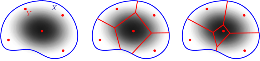
Figure 1. (Left) The domain $X$ (with boundary in blue) is endowed with a probability density pictured in grayscale representing the density of population in a city. The set $Y$ (in red) represents the location of bakeries. Here, $X,Y\subseteq\mathbb{R}^{2}$ and $c(x,y)=|x-y|^{2}$ (Middle) The Voronoi tessellation induced by the bakeries (Right) The Laguerre tessellation: the price of bread the bakery near the center of $X$ is higher than at the other bakeries, effectively shrinking its Laguerre cell.

We will also frequently consider the following hypersurfaces/halfspaces:

$$H_{yz}(\psi) =\{x\in\Omega_{X}\mid c(x,y)+\psi(y)=c(x,z)+\psi(z)\},$$ (4.51)

$$H^{\leqslant}_{yz}(\psi) =\{x\in\Omega_{X}\mid c(x,y)+\psi(y)\leqslant c(x,z)+\psi(z)\},$$

which are defined so that

$$\forall y\in Y,\mathrm{Lag}_{y}(\psi)=\cap_{z\in Y\setminus\{y\}}H_{yz}^{\leqslant}(\psi)$$ (4.52)

$$\forall y,z\in Y,\mathrm{Lag}_{yz}(\psi)\subseteq H_{yz}(\psi)$$

Remark 17.

For the quadratic cost $c(x,y)=\left\|x-y\right\|^{2}$, one has

$$c(x,y)+\psi(y)\leqslant c(x,z)+\psi(z)$$

$$\Longleftrightarrow\langle x|z-y\rangle\leqslant\frac{1}{2}(\psi(z)+\left\|z\right\|^{2}-(\psi(y)-\left\|y\right\|^{2})),$$

which easily implies that the Laguerre cells are convex polyhedra intersected with the domain $\Omega_{X}$. Introducing $\tilde{\psi}(z)=\frac{1}{2}(\psi(z)+\left\|z\right\|^{2})$, one has

$$\mathrm{Lag}_{y}(\psi)=\{x\in\Omega_{X}\mid\forall z\in Y,~{}\langle x|z-y\rangle\leqslant\tilde{\psi}(z)-\tilde{\psi}(y)\}.$$

As a direct consequence, the intersection of two distinct Laguerre cells is contained in an hyperplane and is therefore Lebesgue negligible. If in addition $\psi\equiv 0$, then the Laguerre tessellation coincides with the Voronoi tessellation. The shape of the Voronoi and Laguerre tessellations is depicted in Figure 1.

The following proposition shows that Laguerre tessellations can be used to build optimal transport maps.

Proposition 37.

Under the twist condition (Def. 8), the intersection of two distinct Laguerre cells $\mathrm{Lag}_{y}(\psi)\cap\mathrm{Lag}_{z}(\psi)$ ($y\neq z$) is Lebesgue-negligible, and the map

$$T_{\psi}:x\in\Omega_{X}\mapsto\arg\min_{y\in Y}c(x,y)+\psi(y)$$

is well-defined Lebesgue almost-everywhere. In addition for any $\psi\in\mathbb{R}^{Y}$ and any $\rho\in\mathcal{P}^{\mathrm{ac}}(X)$, $T_{\psi}$ is an optimal transport map for the cost $c$ between $\rho$ and the measure

$$\nu_{\psi}:=T_{\psi\#}\rho=\sum_{y\in Y}\rho(\mathrm{Lag}_{y}(\psi))\delta_{y}.$$ (4.53)

Proof.

By Equation (4.52), one has

$$\mathrm{Lag}_{y}(\psi)\cap\mathrm{Lag}_{z}(\psi)=\mathrm{Lag}_{yz}(\psi)\subseteq f^{-1}(\{0\}),$$

where we have set $f(x)=c(x,y)-c(x,z)+\psi(y)-\psi(z)$. By the twist condition, $\nabla f(x)\neq 0$ for all $x\in\Omega_{X}$, implying that the set $f^{-1}(\{0\})$ is a $(d-1)$-submanifold and is in particular Lebesgue-negligible. This easily implies that $T_{\psi}$ is well-defined.

Let us now prove optimality of $T_{\psi}$ in the optimal transport problem between $\rho$ and $T_{\psi\#}\rho$. By definition of $T_{\psi}$, one has

$$\forall(x,y)\in X,~{}~{}c(x,T_{\psi}(x))+\psi(T_{\psi}(x))\leqslant c(x,y)+\psi(y).$$

Let $\gamma$ be a transport plan between $\rho$ and $\nu_{\psi}$. Integrating the above inequality with respect to $\gamma$ gives

$$\int_{X}(c(x,T_{\psi}(x))+\psi(T_{\psi}(x)))\rho(x)\mathrm{d}x\leqslant\int_{X\times Y}(c(x,y)+\psi(y))\mathrm{d}\gamma(x,y),$$

where we have used $\Pi_{X\#}\gamma=\rho$ to simplify the left-hand side. Since $\nu=\Pi_{Y\#}\gamma=T_{\psi\#}\rho$, applying change of variable formulas we get

$$\int_{X\times Y}\psi(y)\mathrm{d}\gamma(x,y)=\int_{Y}\psi(y)\mathrm{d}\nu=\int_{X}\psi(T_{\psi}(x))\rho(x)\mathrm{d}x$$

Substracting this equality from the inequality above shows that the map $T_{\psi}$ is optimal in the optimal transport :

$$\int_{X}c(x,T_{\psi}(x))\rho(x)\mathrm{d}x\leqslant\int_{X\times Y}c(x,y)\mathrm{d}\gamma(x,y)\qed$$

Monge-Ampère equation

Proposition 37 implies that any map $T_{\psi}$ induced by a Laguerre tessellation of the domain solves the optimal transport between $\rho$ and the image measure $\nu_{\psi}=T_{\psi\#}\rho$. From now on, we will denote

$$G_{y}:\mathbb{R}^{Y}\to\mathbb{R},\psi\mapsto\rho(\mathrm{Lag}_{y}(\psi))$$ (4.54)

$$G:\mathbb{R}^{Y}\to\mathbb{R}^{Y},\psi\mapsto(y\mapsto G_{y}(\psi)).$$

In the bakery analogy, the function $G_{y}(\psi)$ measures the number of customers for the bakery $y$ given a family of prices $\psi\in\mathbb{R}^{Y}$, and $G:\mathbb{R}^{Y}\to\mathbb{R}^{Y}$ maps a family of prices to a distribution of customers among the bakeries. By (4.53), one has

$$\nu_{\psi}=\sum_{y\in Y}G_{y}(\psi)\delta_{y}.$$

For simplicity, we consider $\mathcal{P}(Y)$ as a subset of $\mathbb{R}^{Y}$, conflating a probability measure $\nu=\sum_{y\in Y}\nu_{y}\delta_{y}$ with the function $\nu:y\mapsto\nu_{y}$. Then, $T_{\psi}$ is an optimal transport map between $\rho$ and $\nu$ iff $T_{\psi\#}\rho=\nu$ iff

$$G(\psi)=\nu.$$ (4.55)

In other words, we have transformed the optimal transport problem into a finite-dimensional non-linear system of equations (4.55).

Remark 18 (Relation to subdifferential and Monge-Ampère equation).

Assume that $X=\Omega_{X}=\mathbb{R}^{d}$ and that $c(x,y)=-\langle x|y\rangle$. Then,

$$\mathrm{Lag}_{y}(\psi) =\{x\in\Omega_{X}\mid\forall z\in Y,~{}-\langle x|y\rangle+\psi(y)\leqslant-\langle x|z\rangle+\psi(z)\}$$

$$=\{x\in\Omega_{X}\mid\forall z\in Y,~{}\psi(z)\geqslant\langle x|z-y\rangle+\psi(y)\}$$

Denote $\hat{\psi}$ the convex envelope of $\psi$, which can be defined using the double Legendre-Fenchel transform by

$$\varphi(x)=\max_{y\in Y}\langle x|y\rangle-\psi(y),$$

$$\hat{\psi}(z)=\max_{x\in X}\langle x|y\rangle-\varphi(x).$$

Then the Laguerre cells defined above agree with the subdifferential of $\hat{\psi}$, i.e. $\mathrm{Lag}_{y}(\psi)=\partial\hat{\psi}(y).$ Moreover, in the context of Monge-Ampère equations, the (infinite) measure

$$\sum_{y\in Y}\lambda(\mathrm{Lag}_{y}(\psi))\delta_{y}=\sum_{y\in Y}\lambda(\partial\hat{\psi}(y))\delta_{y}$$

is called the Monge-Ampère measure of the function $\hat{\psi}$ [57]. Semi-discrete techniques can also be applied to the numerical resolution of Monge-Ampère equations (with e.g. Dirichlet boundary conditions). We refer the reader to the pioneering work of Oliker-Prussner [79] and to the survey by Neilan, Salgado and Zhang [77].

Remark 19 (Lack of uniqueness).

The solution $\psi$ to $G(\psi)=\nu$ is never unique, because $G$ is invariant under addition of a constant (see Proposition 38-(iii)). When $\mathrm{spt}(\rho)$ is disconnected there might also exist two solutions $\psi^{0},\psi^{1}$ to $G(\psi^{i})=\nu$ such that $\psi^{0}-\psi^{1}$ is not constant. Take $X=[-1,1]$, $Y=\{-1,1\}$, choose $c(x,y)=(x-y)^{2}$ and

$$\rho=\mathbf{1}_{[-1,-\frac{1}{2}]\cup[\frac{1}{2},1]}\qquad\nu=\frac{1}{2}(\delta_{-1}+\delta_{1}),$$

A computation shows that if $\left|\psi(1)-\psi(-1)\right|\leqslant 2$, then $G(\psi)=\nu$.

The existence of solutions to (4.55) and the algorithms that one can use to solve this system depend crucially on the properties of the function $G$. In the next proposition, we denote $(\mathbf{1}_{y})_{y\in Y}$ the canonical basis of $\mathbb{R}^{Y}$, i.e. $\mathbf{1}_{y}(z)=1$ if $y=z$ and $0$ if not. We also denote $\mathbf{1}_{Y}$ the constant function on $Y$ equal to $1$. On $\mathbb{R}^{Y}$ we consider two norms:

$$\left\|\psi\right\|=\sqrt{\sum_{y\in Y}\left|\psi(y)\right|^{2}}\quad\hbox{ and }\quad\left\|\psi\right\|_{\infty}=\max_{y\in Y}\left|\psi(y)\right|.$$

We will often use the notation $R$, which measures the oscillation of the cost function:

$$R:=\max_{X\times Y}c-\min_{X\times Y}c,$$ (4.56)

Proposition 38.

Assume $c$ is twisted (Def. 8) and $\rho\in\mathcal{P}^{\mathrm{ac}}(X)$. Then,

1. $\forall y\in Y,\forall t\geqslant 0$, $G_{y}(\psi+t\mathbf{1}_{y})\leqslant G_{y}(\psi)$,

2. $\forall y\neq z\in Y,\forall t\geqslant 0$, $G_{y}(\psi+t\mathbf{1}_{z})\geqslant G_{y}(\psi)$,

3. $\forall\psi\in\mathbb{R}^{Y},\forall t\in\mathbb{R},~{}G(\psi+t\mathbf{1}_{Y})=G(\psi)$,

4. $\forall\psi\in\mathbb{R}^{Y},G(\psi)\in\mathcal{P}(Y)$,

5. if $\psi\in\mathbb{R}^{Y}$ is such that $G_{y_{0}}(\psi)>0$, then $\psi(y_{0})\leqslant\min_{Y}\psi+R$,

6. if $\psi\in\mathbb{R}^{Y}$ is such that $G_{y}(\psi)>0$ for every $y\in Y$, then
   $\max_{Y}\psi-\min_{Y}\psi\leqslant R$,

7. $G$ is continuous,

where $R=\max_{X\times Y}c-\min_{X\times Y}c$.

Proof.

The properties (i), (ii), (iii) are straightforward consequences of the definition of Laguerre cells. Property (iv) is a consequence of Proposition 37 and of the assumption $\rho\in\mathcal{P}^{\mathrm{ac}}(X)$. To prove (v), take $\psi$ such that $G_{y_{0}}(\psi)>0$, implying in particular that the Laguerre cell $\mathrm{Lag}_{y_{0}}(\psi)$ is non-empty and contains a point $x\in X$. Then, by definition of the cell one has for all $y\in Y\setminus\{y_{0}\}$, $c(x,y_{0})+\psi(y_{0})\leqslant c(x,y)+\psi(y),$ thus showing that $\psi(y_{0})\leqslant\min_{Y}\psi+R$. Point (v) is a consequence of Point (vi).

It remains to establish that each of the maps $G_{y}$ is continuous. For this purpose, we consider a sequence $(\psi_{n})_{n\in\mathbb{N}}\in\mathbb{R}^{Y}$ converging to some $\psi_{\infty}\in\mathbb{R}^{Y}$. We first note that as in the proof of Proposition 37, the set

$$S=\{x\in X\mid\exists y\neq z\in Y\hbox{ s.t. }c(x,y)+\psi(y)=c(x,y)+\psi(z)\}.$$

is Lebesgue-negligible and therefore also $\rho$-negligible. Defining $\chi=\mathbf{1}_{\mathrm{Lag}_{y}(\psi)}$ and $\chi_{n}=\mathbf{1}_{\mathrm{Lag}_{y}(\psi_{n})}$,

$$G_{y}(\psi_{n})=\int\chi_{n}\mathrm{d}\rho,\hbox{ and }G(\psi)=\int\chi\mathrm{d}\rho.$$

To prove that $\lim_{n\to+\infty}G_{y}(\psi_{n})=G_{y}(\psi)$ it suffices to establish that $\chi_{n}$ converges to $\chi$ on $X\setminus S$, which is straightforward (because the inequalities defining the set $X\setminus S$ are strict), and to apply Lebesgue’s dominated convergence theorem. ∎

From these properties of $G$, we can deduce the existence of a solution to the equation $G(\psi)=\nu$. The strategy used to prove this proposition is borrowed from [24] and is also reminiscent of Perron’s method to prove existence to Monge-Ampère equations, see e.g. [57].

Corollary 39.

Let $G:\mathbb{R}^{Y}\to\mathbb{R}^{Y}$ satisfying (i)– (vi) in Proposition 38 and let $\nu\in\mathcal{P}(Y)$. Then, there exists $\psi\in\mathbb{R}^{Y}$ such that $G(\psi)=\nu$.

Proof.

Fix some $y_{0}\in Y$ such that $\nu_{y_{0}}\neq 0$, and consider the set

$$K=\{\psi\in\mathbb{R}^{Y}\mid\psi(y_{0})=0\hbox{ and }\forall y\in Y\setminus\{y_{0}\},G_{y_{0}}(\psi)\leqslant\nu_{y}\hbox{ and }\psi(y)\leqslant R\},$$

where $R$ is defined as in (4.56). Given $\psi\in K$, one has

$$G_{y_{0}}(\psi)=1-\sum_{y\neq y_{0}}G_{y}(\psi)\geqslant\nu_{y_{0}}>0,$$

implying by (v) that $\min_{y\in Y}\psi\geqslant\psi(y_{0})-R$. The set $K$ is therefore bounded and closed (by continuity of the functions $G_{y}$) and therefore compact. We consider $\psi^{*}$ a minimizer over the set $K$ of the function $J(\psi)=\sum_{y\in Y}\psi_{y}$. Assume that $G_{y}(\psi^{*})<\nu_{y}$ for some $y\in Y\setminus\{y_{0}\}$. Then, by continuity of $G_{y}$, there exists some $t>0$ such that $G_{y}(\psi^{*}-t\mathbf{1}_{y})<\nu_{y}$. Then, by property (ii), we have

$$\forall z\neq y,G_{z}(\psi^{*}-t\mathbf{1}_{y})\leqslant G_{z}(\psi^{*})\leqslant\nu_{z},$$

thus showing that $\psi^{*}-t\mathbf{1}_{y}\in K$. Since $J(\psi^{*}-t\mathbf{1}_{y})=J(\psi^{*})-t<J(\psi^{*})$, we get a contradiction. We thus have showed that $\forall y\in Y\setminus\{y_{0}\},$ $G_{y}(\psi^{*})=\nu_{y}$, and using (iv) and $\nu\in\mathcal{P}(Y)$ we obtain

$$G_{y_{0}}(\psi^{*})=1-\sum_{y\in Y\setminus\{y_{0}\}}G_{y}(\psi^{*})=1-\sum_{y\in Y\setminus\{y_{0}\}}\nu_{y}=\nu_{y_{0}},$$

so that $G(\psi^{*})=\nu$ and $\psi^{*}$ is a solution to (4.55). ∎

Kantorovich’s functional

We now show that Equation (4.55) is the optimality condition of the Kantorovitch functional, and can thus be recast as a smooth unconstrained optimization problem. We recall that

$$\mathrm{(KP)}=\max_{\psi\in\mathbb{R}^{Y}}\mathcal{K}(\psi),$$

where $\mathcal{K}$ is the Kantorovich functional given by

$$\mathcal{K}(\psi) =\int_{X}\psi^{c}\mathrm{d}\mu-\int_{Y}\psi\mathrm{d}\nu$$

$$=\sum_{y\in Y}\int_{\mathrm{Lag}_{y}(\psi)}(c(x,y)+\psi(y))\mathrm{d}\rho(x)-\sum_{y\in Y}\psi(y)\nu_{y}.$$

Theorem 40 (Aurenhammer, Hoffman, Aronov).

Assume that $\rho\in\mathcal{P}^{\mathrm{ac}}(X)$, that $c$ is twisted (Def. 8), and consider $\mathcal{K}$ defined in (2.24). Then:

• $\mathcal{K}$ is concave and $\mathcal{C}^{1}$-smooth and its gradient is

  $$\nabla\mathcal{K}(\psi)=G(\psi)-\nu$$ (4.57)

  where $G$ is defined in (4.54).

• $\forall\psi\in\mathbb{R}^{Y},\forall t\in\mathbb{R},~{}\mathcal{K}(\psi+t\mathbf{1}_{Y})=\mathcal{K}(\psi)$,

• $\mathcal{K}$ attains its maximum over $\mathbb{R}^{Y}$, and $\nabla\mathcal{K}(\psi)=0$ iff $\psi$ solves (4.55).

Remark 20.

This theorem could be deduced from the computation of directional derivatives of $\mathcal{K}$ given in Corollary 16, however we prefer to give a simple and self-contained proof due to Aurenhammer, Hoffman, Aronov [6].

Proof of Theorem 40.

We simultaneously show that the functional is concave and compute its gradient. For any function $\psi$ on $Y$ and any measurable map $T:X\to Y$, one has

$$\min_{y\in Y}(c(x,y)+\psi(y))\leqslant c(x,T(x))+\psi(T(x)),$$

which by integration against $\rho$ gives

$$\mathcal{K}(\psi)\leqslant\int_{X}(c(x,T(x))+\psi(T(x)))\rho(x)\mathrm{d}x-\sum_{y\in Y}\psi(y)\nu_{y}.$$ (4.58)

Moreover, equality holds when $T=T_{\psi}$. Taking another function $\psi^{\prime}\in\mathbb{R}^{Y}$ and setting $T=T_{\psi^{\prime}}$ in Equation (4.58) gives

$$\mathcal{K}(\psi) \leqslant\int_{X}(c(x,T_{\psi^{\prime}}(x))+\psi(T_{\psi^{\prime}}(x)))\rho(x)\mathrm{d}x-\sum_{y\in Y}\psi(y)\nu_{y}$$

$$=\sum_{y\in Y}\int_{\mathrm{Lag}_{y}(\psi^{\prime})}(c(x,y)+\psi(y))\rho(x)\mathrm{d}x-\sum_{y\in Y}\psi(y)\nu_{y}$$

$$=\sum_{y\in Y}\int_{\mathrm{Lag}_{y}(\psi^{\prime})}(c(x,y)+\psi^{\prime}(y))\rho(x)\mathrm{d}x+$$

$$\phantom{=}\sum_{y\in Y}\rho(\mathrm{Lag}_{y}(\psi^{\prime}))(\psi(y)-\psi^{\prime}(y))-\sum_{y\in Y}\psi(y)\nu_{y}$$

$$=\mathcal{K}(\psi^{\prime})+\langle G(y)-\nu|\psi-\psi^{\prime}\rangle$$

By definition, this shows that $G(\psi)-\nu$ belongs to the superdifferential to $\mathcal{K}$ (Definition 21) at $\psi$, i.e. $G(\psi)-\nu\in\partial^{+}\mathcal{K}(\psi)$, thus proving by Proposition 55 that $\mathcal{K}$ is concave.

We now prove that $\mathcal{K}$ belongs to $\mathcal{C}^{1}(\mathbb{R}^{Y})$. Consider $\psi\in\mathbb{R}^{Y}$ and let $(\psi_{n})_{n\in\mathbb{N}}$ be a sequence converging to $\psi$ and such that $\nabla\mathcal{K}(\psi_{n})$ exists for every $n\in\mathbb{N}$. Since $G(\psi_{n})-\nu\in\partial^{+}\mathcal{K}(\psi_{n})=\{\nabla\mathcal{K}(\psi_{n})\},$ we obtain $\nabla\mathcal{K}(\psi_{n})=G(\psi_{n})-\nu$. Thus, by the continuity of $G$ (Proposition 38),

$$\lim_{n\to+\infty}\nabla\mathcal{K}(\psi_{n})=\lim_{n\to+\infty}G(\psi_{n})-\nu=G(\psi)-\nu,$$

ensuring by (5.76) that $\partial^{+}G(\psi)=\{G(\psi)-\nu\}$, so that $\nabla\mathcal{K}(\psi)=G(\psi)-\nu$ for all $\psi\in\mathbb{R}^{Y}$. By continuity of $G$ we get $\mathcal{K}\in\mathcal{C}^{1}$ as announced, and Equation (4.54) holds for all $\psi\in\mathbb{R}^{Y}$, so that one trivially has $\nabla\mathcal{K}(\psi)=0$ iff $G(\psi)=\nu$. Finally, we note that thanks to Corollary 39, there exists $\psi\in\mathbb{R}^{Y}$ such that $G(\psi)=\nu$, which automatically is a maximizer of $\mathcal{K}$ because $\mathcal{K}$ is concave and $\nabla\mathcal{K}(\psi)=0$. ∎

4.2. Semi-discrete optimal transport via coordinate decrements

As before, we assume that $X\subseteq\Omega_{X}$ is compact, that $Y\subseteq\Omega_{Y}$ is finite and that $\Omega_{X},\Omega_{Y}\subseteq\mathbb{R}^{d}$ are open sets. We recall the notation $G_{y}(\psi):=\rho(\mathrm{Lag}_{y}(\psi)).$ Oliker-Prussner’s algorithm for solving $G(\psi)=\nu$ is described in Algorithm 3, and bears strong resemblance with Bertsekas’ auction algorithm, in that the “prices” are evolved in a monotonic way.

Input:

A tolerence parameter $\delta>0$.

Initialization:

Fix some $y_{0}\in Y$ once for all. Set

$$\psi^{(0)}(y):=\begin{cases}0&\hbox{ if }y=y_{0}\\ R&\hbox{ if not}.\end{cases}$$

While:

$\exists y\neq y_{0}$ such that $G_{y}(\psi^{(k)}))\leqslant\nu_{y}-\frac{\delta}{N}$

Step 1:

Compute

$$t_{y}=\min\{t\geqslant 0\mid G_{y}(\psi^{(k)}-t\mathbf{1}_{y})\geqslant\nu_{y}\}.$$ (4.59)

Step 2:

Set $\psi^{(k+1)}=\psi^{(k)}-t\mathbf{1}_{y}$.

Output:

A vector $\psi^{(k)}$ that satisfies $\left\|G(\psi^{(k)})-\nu\right\|_{\infty}\leqslant\delta$.

Algorithm 3 Oliker-Prussner algorithm

This algorithm can be described in words using the bakery analogy of Section 4.1. We choose once and for all a bakery $y_{0}\in Y$ whose price will be set to zero. Initially, the price of bread $\psi^{(0)}$ is zero at this bakery $y_{0}$ and set to the prohibitively large value $R$, defined in Equation (4.56), at any other location. This choice guarantees that the bakery $y_{0}$ initially gets all the customers. The prices $\psi^{(k)}\in\mathbb{R}^{y}$ are then constructed iteratively by performing a sort of reverse auction: at step $k$, start by finding some bakery $y=y^{(k)}\in Y\setminus\{y_{0}\}$ which sells less bread than its production capacity, i.e.

$$G_{y}(\psi^{(k)})\leqslant\nu_{y}-\frac{\delta}{N}.$$

The price of bread at $y$ is then decreased so that the amount of bread sold equals the production capacity of $y$, i.e. one finds $t_{y}\geqslant 0$ such that

$$G_{y}(\psi^{(k)}-t_{y}\mathbf{1}_{y})=\nu_{y}$$

and then updates $\psi^{(k+1)}=\psi^{(k)}-t_{y}\mathbf{1}_{y}$.

Remark 21 (Origin and extensions).

This algorithm was introduced by Oliker and Prussner, for the purpose of solving Monge-Ampère equations with Dirichlet boundary conditions in [79]. In the context of optimal transport, the first use of Algorithm 3 seems to be in an article of Caffarelli, Kochengin and Oliker [26] (see also [24]), in the setting of the reflector problem, namely $c(x,y)=-\log(1-\langle x|y\rangle)$ on $X=Y=\mathcal{S}^{d-1}$. Since then, the convergence of this algorithm has been generalized to more other costs and/or more general assumptions on the probability density $\rho$, we refer the reader to [64, 42] and to references therein.

$\mathcal{C}^{1,1}$ estimates for Kantorovich functional

The proof of convergence of Oliker-Prussner’s algorithm relies on the Lipschitz regularity of the map $G$ when $\rho$ is bounded, proven in the next proposition. (Since $\nabla\mathcal{K}=G-\nu$, this proposition also implies that Kantorovich’s functional $\mathcal{K}$ has Lipschitz gradient, improving from the $\mathcal{C}^{1}$ estimate of Theorem 40.)

Proposition 41.

Assume that $c\in\mathcal{C}^{2}(\Omega_{X}\times\Omega_{Y})$ satisfies the twist condition, and assume also that $\rho\in\mathcal{P}^{\mathrm{ac}}(X)\cap\mathrm{L}^{\infty}(X)$. Then for every $y\in Y$, the map $G_{y}:\mathbb{R}^{Y}\to\mathbb{R}$ defined in (4.54) is globally Lipschitz.

Remark 22.

The proof of this proposition comes with an estimation of the Lipschitz constant: namely it shows $\left|G_{y}(\psi)-G_{y}(\varphi)\right|\leqslant L_{G}\left\|\varphi-\psi\right\|_{\infty}$ with

$$L_{G}=c(d)N\left\|\rho\right\|_{\infty}\frac{1}{\kappa}\left(1+\frac{M}{\kappa}\operatorname{diam}(X)\right)\operatorname{diam}(X)^{d-1},$$ (4.60)

$$\kappa=\min_{y\neq z\in Y}\min_{X}\left\|\nabla_{x}c(\cdot,y)-\nabla_{x}c(\cdot,z)\right\|,$$

$$M=\max_{y\neq z\in Y}\max_{X}\left\|\mathrm{D}^{2}_{xx}c(\cdot,y)-\mathrm{D}^{2}_{xx}c(\cdot,z)\right\|.$$

In the estimation of the Lipschitz constant $L_{G}$ (4.60), it is possible that the term in $N$ is not tight, but the other terms cannot be improved without adding assumptions on the cost.

Example 6.

With $c(x,y)=\frac{1}{2}\left\|x-y\right\|^{2}$, one has $\nabla_{x}c(x,y)=(x-y)$ and $\mathrm{D}^{2}_{xx}c(x,y)=\mathrm{id}$, so that $M=0$ and $\kappa$ is the minimal distance between two distinct points in $Y$: $\kappa=\min_{y\neq z\in Y}\left\|y-z\right\|.$

The proof relies on the following lemma, which allows to estimate the variations of $G_{y}$ in the direction $\mathbf{1}_{z}$, $z\neq y$.

Lemma 42.

Let $c\in\mathcal{C}^{1}(\Omega_{X}\times\Omega_{Y})$ be a twisted cost and $\rho\in\mathcal{P}^{\mathrm{ac}}(X)$. For every $y\neq z\in Y$ and $\psi\in\mathbb{R}^{Y}$,

$$G_{y}(\psi+t\mathbf{1}_{z})-G_{y}(\psi)=\int_{0}^{t}G_{yz}(\psi+s\mathbf{1}_{z})\mathrm{d}s.$$ (4.61)

where

$$G_{yz}(\psi)=\int_{\mathrm{Lag}_{yz}(\psi)}\frac{\rho(x)}{\left\|\nabla_{x}c(y,x)-\nabla_{x}c(y,z)\right\|}\mathrm{d}\mathrm{vol}^{d-1}(x).$$

Proof.

This is a consequence of the coarea formula, Equation (5.78). In order to see this, we first note that

$$\mathrm{Lag}_{y}(\psi+t\mathbf{1}_{z})=E\cap H^{\leqslant}_{yz}(\psi)\quad\hbox{ where }E=\bigcap_{w\in Y\setminus\{y,z\}}H_{yw}^{\leqslant}(\psi).$$

In particular, for $t\geqslant 0$, setting $c_{yz}=c(\cdot,y)-c(\cdot,z)$ and $a=\psi(z)-\psi(y)$,

$$\mathrm{Lag}_{y}(\psi+t\mathbf{1}_{z})\setminus\mathrm{Lag}_{y}(\psi)=E\cap c_{yz}^{-1}((a,a+t])$$

Thus, by the coarea formula,

$$G_{y}(\psi+t\mathbf{1}_{z})-G_{y}(\psi) =\rho(\mathrm{Lag}_{y}(\psi+t\mathbf{1}_{z})\setminus\mathrm{Lag}_{y}(\psi))$$

$$=\int_{E\cap c_{yz}^{-1}((a,a+t])}\rho(x)\mathrm{d}\operatorname{vol}^{d}(x)$$

$$=\int_{0}^{t}\int_{E\cap c_{yz}^{-1}(a+s)}\frac{\rho(x)}{\left\|\nabla c_{yz}(x)\right\|}\mathrm{d}\mathrm{vol}^{d-1}(x)\mathrm{d}s$$

One concludes by remarking that

$$x\in\mathrm{Lag}_{yz}(\psi+s\mathbf{1}_{z}) \Longleftrightarrow x\in E\hbox{ and }c(x,y)+\psi(y)=c(x,z)+\psi(z)+s$$

$$\Longleftrightarrow x\in E\cap c_{yz}^{-1}(a+s).$$

This establishes (4.61) in the case $t\geqslant 0$, and the case $t\leqslant 0$ can be treated similarly. ∎

The second ingredient to prove Proposition 41 is an uniform upper bound on the $(d-1)$–Hausdorff measure of the level set of a $\mathcal{C}^{2}$ function $f$ with non-vanishing gradient.

Lemma 43.

Let $X\subseteq\Omega_{X}\subseteq\mathbb{R}^{d}$ with $\Omega_{X}$ open and $X$ compact, and let $f\in\mathcal{C}^{2}(\Omega_{X})$ such that $\forall x\in\Omega_{X},\left\|\nabla f(x)\right\|>0$. Then,

$$\mathrm{vol}^{d-1}(f^{-1}(0)\cap X)\leqslant c(d)\left(1+\frac{M}{\kappa}\operatorname{diam}(X)\right)\operatorname{diam}(X)^{d-1}.$$

where $\kappa=\min_{X}\left\|\nabla f\right\|$ and $M=\max_{X}\left\|\mathrm{D}^{2}f\right\|$.

Proof.

By compactness, there exists a finite number of unit vectors $u_{1},\ldots u_{n}$ and $V_{1},\ldots,V_{n}$ an open covering of the unit sphere $\mathcal{S}^{d-1}$ such that if $u\in V_{i}$, then $\langle u|u_{i}\rangle\geqslant 3/4$, implying in particular, $\left\|u-u_{i}\right\|^{2}=2-2\langle u|u_{i}\rangle\leqslant\frac{1}{2}$. Moreover $n$ depends only on the dimension $d$. Let $S=f^{-1}(0)\cap X$. This set $S$ can be covered by patches $S_{i}$, i.e. $S=\cup_{i}S_{i}$ where

$$S_{i}=\{x\in S\mid\nabla f(x)\in V_{i}\}.$$

We will now estimate the volume of each patch $S_{i}$ using the coarea formula recalled in Theorem 56 of the appendix. To apply this formula, we consider $\Pi_{i}:S_{i}\subseteq\mathbb{R}^{d}\to\{u_{i}\}^{\perp}$ the orthogonal projection onto the hyperplane $H_{i}=\{u_{i}\}^{\perp}$. We need to estimate the Jacobian $J_{\Pi_{i}}(x)$ (see (5.77)). Since $\Pi_{i}$ is linear, we have $\mathrm{D}\Pi_{i}=\Pi_{i}$. Moreover, for any tangent vector $v$ at $x\in S_{i}$, one has $\langle v|\nabla f(x)\rangle=0$. Setting $u=\nabla f(x)\in V_{i}$, we get

$$\left\|\Pi_{i}v\right\|^{2} =\left\|v\right\|^{2}-\langle v|u_{i}\rangle^{2}$$

$$=\left\|v\right\|^{2}-\langle v|u_{i}-u\rangle^{2}$$

$$\geqslant\left\|v\right\|^{2}(1-\left\|u_{i}-u\right\|^{2})\geqslant\frac{1}{2}\left\|v\right\|^{2}.$$

This directly shows that the restriction of $\mathrm{D}\Pi_{i}(x)$ to the tangent space $T_{x}S_{i}$ at $S_{i}$ is injective and that its inverse is $\frac{1}{\sqrt{2}}$-Lipschitz. This implies that

$$J_{\Pi_{i}}(x)\geqslant c(d)=\left(\frac{1}{\sqrt{2}}\right)^{d-1}.$$

We now apply the co-area formula (5.78) to the manifold $M=f^{-1}(0)$, $E=S_{i}\subseteq N$, $N=H_{i}$, $n=m=d-1$, $\Phi=\Pi_{i}$, and $u\equiv 1$:

$$\mathrm{vol}^{d-1}(S_{i}) =\int_{H_{i}}\int_{\Pi_{i}^{-1}(y)}\frac{1}{\mathrm{J}_{\Pi_{i}}(x)}\mathrm{d}\mathrm{vol}^{0}(x)\mathrm{d}\mathrm{vol}^{d-1}(y)$$

$$\leqslant c(d)\int_{\{u_{i}\}^{\perp}}\mathrm{Card}(S_{i}\cap(y+\mathbb{R}u_{i}))\mathrm{d}\mathrm{vol}^{d-1}(y).$$

We now give an upper bound on $\mathrm{Card}(S_{i}\cap(y+\mathbb{R}u_{i}))$. Let $x\in S_{i}$ and use Taylor’s formula to get

$$f(x+tu_{i})\geqslant f(x)+t\langle\nabla f(x)|u_{i}\rangle-\frac{M}{2}t^{2}\geqslant\frac{3}{4}\kappa t-\frac{M}{2}t^{2}$$

so that $f(x+tu_{i})>0$ as long as $t\in(0,t^{*})$ with $t^{*}=\frac{3\kappa}{2M}$. One has a similar bound for negative $t$. This directly implies that the number of intersection points between $S_{i}$ and $y+\mathbb{R}u_{i}$ is at most $1+\operatorname{diam}(X)/t^{*}$. Since the number $n$ of directions $u_{i}$ only depends on the dimension $d$, we have

$$\mathrm{vol}^{d-1}(S) \leqslant\sum_{1\leqslant i\leqslant n}\mathrm{vol}^{d-1}(S_{i})$$

$$\leqslant c(d)\sum_{1\leqslant n}\mathrm{vol}^{d-1}(H_{i}\cap\Pi_{i}(X))\left(1+\frac{M}{\kappa}\operatorname{diam}(X)\right)$$

$$\leqslant c(d)\left(1+\frac{M}{\kappa}\operatorname{diam}(X)\right)\operatorname{diam}(X)^{d-1}.\qed$$

Proof of Proposition 41.

Let $y\in Y$. Applying Lemma 42, we have

$$\left|G_{y}(\psi+t\mathbf{1}_{y})-G_{y}(\psi)\right| \leqslant\left|\int_{0}^{t}\int_{\mathrm{Lag}_{yz}(\psi+s\mathbf{1}_{y})}\frac{\rho(x)}{\left\|\nabla c_{yz}(x)\right\|}\mathrm{d}\mathrm{vol}^{d-1}(x)\mathrm{d}s\right|$$

$$\leqslant\frac{\left\|\rho\right\|_{\infty}}{\kappa}\max_{a\leqslant s\leqslant a+t}\mathrm{vol}^{d-1}(c_{yz}^{-1}(s)\cap X)\left|t\right|,$$

where we used the bound $\left\|\nabla c_{yz}(x)\right\|\geqslant\kappa$, which comes from the twist assumption and the inclusion $\mathrm{Lag}_{yz}(\psi+s\mathbf{1}_{z})\subseteq c_{yz}^{-1}(a+s)$ with $a=\psi(z)-\psi(y)$, as in the proof of the previous lemma. Applying Lemma 43 to the function $f=c_{yz}-s$, we get a uniform upper bound on the $(d-1)$-volume of the level set $c_{yz}^{-1}(s)$:

$$\mathrm{vol}^{d-1}(c_{yz}^{-1}(s)\cap X)\leqslant c(d)\left(1+\frac{M}{\kappa}\operatorname{diam}(X)\right)\operatorname{diam}(X)^{d-1},$$

which yields

$$\left|G_{y}(\psi+t\mathbf{1}_{z})-G_{y}(\psi)\right|\leqslant\hat{L}_{G}\left|t\right|,$$ (4.62)

$$\hbox{ with }\hat{L}_{G}=\frac{c(d)}{\kappa}\left(1+\frac{M}{\kappa}\operatorname{diam}(X)\right)\operatorname{diam}(X)^{d-1}\ \|\rho\|_{\infty}.$$

Take $\psi,\tilde{\psi}\in\mathbb{R}^{Y}$. Order the points in $Y$, i.e. let $Y=\{y_{1},\ldots,y_{N}\}$ and define recursively

$$\begin{cases}\psi^{0}=\psi\\ \psi^{k+1}=\psi^{k}+(\tilde{\psi}(y_{k})-\psi(y_{k}))\mathbf{1}_{y_{k}}\end{cases}$$

Then, $\psi^{N}=\tilde{\psi}$ and for $k\geqslant 1$, $\psi^{k+1}$ and $\psi^{k}$ differ only by the value at $y_{k}$ Thus, applying (4.62),

$$\left|G_{y}(\tilde{\psi})-G_{y}(\psi)\right| =\sum_{1\leqslant k\leqslant N}\left|G_{y}(\psi^{k+1})-G_{y}(\psi^{k})\right|$$

$$\leqslant\sum_{1\leqslant k\leqslant N}\hat{L}_{G}\left|\psi(y_{k})-\tilde{\psi}(y_{k})\right|$$

$$\leqslant L_{G}\left\|\psi-\tilde{\psi}\right\|_{\infty}\hbox{ with }L_{G}=N\hat{L}_{G}\qed$$

Convergence of Oliker-Prussner’s algorithm

Now that we have established the Lipschitz continuity of $G_{y}$, the convergence of Algorithm 3 follows easily, using arguments similar to those used to establish the convergence of Auction’s algorithm.

Theorem 44 (Oliker-Prussner).

Assume that the cost $c\in\mathcal{C}^{2}(\Omega_{X}\times\Omega_{Y})$ is twisted (Def. 8) and that $\rho\in\mathcal{P}^{\mathrm{ac}}(X)\cap\mathrm{L}^{\infty}(X)$. Then,

• Oliker-Prussner’s algorithm converges in a finite number of steps $k\leqslant\mathrm{C}N^{3}/\delta$, where $\mathrm{C}$ is a constant that depends on $X$, $Y$, $\rho$ and $c$.

• Furthermore, at step $k$, one has

  $$\forall 1\leqslant i\leqslant N,\left|G_{i}(\psi^{(k)})-\nu_{i}\right|\leqslant\delta.$$

Remark 23 (Computational complexity).

The computational complexity is actually much higher than the number of steps of the algorithm, since:

• at each iteration, one needs to compute $t_{y}$ (this could be done using for instance a binary search or more clever techniques).

• each time the map $G_{y}$ is evaluated, one needs to compute the Laguerre cell $\mathrm{Lag}_{y}(\psi)$, which, if done naively, requires to compute the intersection of $N-1$ half-spaces $H^{\leqslant}_{yz}(\psi)$.

Overall, this leads to an upper bound on computational complexity of at least $\operatorname{O}(\frac{N^{4}}{\delta}\log(N))$, assuming that one can compute $\mathrm{Lag}_{y}(\psi)$ in time $N$. To the best of our knowledge, there exists no lower bound on the number of iterations of Algorithm 3, i.e. specific instances of the problem for which one can count the number of iterations.

Remark 24 ($\delta$-Scaling).

It is tempting to perform $\delta$-scaling as in the case of Auction’s algorithm (see Algorithm 2). In practice, one could start with a rather large $\delta^{(0)}\in(0,1)$, to get a first estimation of the prices using Oliker-Prussner’s algorithm. Then one would iteratively replace $\delta^{(\ell)}$ by $\delta^{(\ell+1)}=\frac{1}{2}\delta^{(\ell)}$ and run again the algorithm starting from the prices found at the previous iteration. Doing so, one could hope to get rid of the $\frac{1}{\delta}$ term in the number of iterations, and to replace it by e.g. $\log\left(\frac{1}{\delta}\right)$.

Proof of Theorem 44.

Step 1 (Correctness) When Algorithm 3 terminates with $\psi:=\psi^{(k)}$, one has for any $y\neq y_{0}$, $\rho(\mathrm{Lag}_{y}(\psi))\leqslant\nu_{y}$. When it stops, it also means that one has $\rho(\mathrm{Lag}_{y}(\psi))\geqslant\nu_{y}-\frac{\delta}{N}$. Then, as desired, we get

$$\rho(\mathrm{Lag}_{y_{0}}(\psi))=1-\sum_{y\neq y_{0}}\rho(\mathrm{Lag}_{y_{0}}(\psi))\in[\nu_{y_{0}},\nu_{y_{0}}+\delta].$$

Step 2 (A priori bound on $\psi_{k}$) By construction one has $\rho(\mathrm{Lag}_{y}(\psi^{(k)}))\leqslant\nu_{y}$, which also imply that

$$\rho(\mathrm{Lag}_{y_{0}}(\psi^{(k)}))=1-\sum_{y\in Y\setminus\{y_{0}\}}\rho(\mathrm{Lag}_{y}(\psi^{(k)}))\geqslant\nu_{y_{0}}>0.$$

By Proposition 38–(v), we get $0=\psi^{k}(y_{0})\leqslant\min_{Y}\psi^{(k)}+R$. Since the price of $y_{0}$ is never changed, $\psi^{(k)}(y_{0})=0$ and $R\geqslant\psi^{(k)}\geqslant-R$.

Step 3 (Minimum decrease and termination) In the second step of the algorithm, when $\psi^{(k)}$ is updated one has $G_{y}(\psi^{(k)}-t_{t}\mathbf{1}_{y})\geqslant G_{y}(\psi^{(k)})+\frac{\delta}{N}$. Since $G_{y}$ is Lipschitz with some constant $L_{G}$, this implies that $\left|t_{y}\right|\geqslant\frac{\delta}{NL_{G}}$. Then, since $\psi_{0}(y)=R$ and for any $k$, $\psi_{k}(y)\geqslant-R$, the number of times $k_{y}$ the price of a point $y\in Y$ has been updated cannot be too large:

$$k_{y}\delta/(NL_{G})\leqslant 2R,$$

i.e. $k_{y}\leqslant(2RNL_{G})/\delta$. Since this bound on the number of steps is for a single point, it needs to be multiplied by $N$ to get the total number of steps. Using the bound on $L_{G}$ given in (4.60), we get an upper bound of $\operatorname{O}(\frac{N^{3}}{\delta})$ on the number of iterations of the algorithm. ∎

4.3. Semi-discrete optimal transport via Newton’s method

We consider a simple damped Newton’s algorithm to solve semi-discrete optimal transport problem introduced in [65], and adapted from a similar algorithm for solving Monge-Ampère equations with Dirichlet boundary conditions [75].

Hessian of Kantorovich’s functional

In order to write the Newton’s algorithm, we first show that $G$ is $\mathcal{C}^{1}$ (or equivalently $\mathcal{K}$ is $\mathcal{C}^{2}$) and we compute its derivatives under a genericity assumption, which depends on the cost and on the choice of points $Y$. This condition is a bit technical, but is for instance satisfied for the quadratic cost on $\mathbb{R}^{d}$ (see Remark 27 below).

Definition 18 (Genericity assumption).

Let $\Omega_{X},\Omega_{Y}\subseteq\mathbb{R}^{d}$ open, $c\in\mathcal{C}^{1}(\Omega_{X}\times\Omega_{Y})$, and $X\subseteq\Omega_{X}$, $Y\subseteq\Omega_{Y}$, with $X$ compact and $Y$ finite.

• We call $Y$ generic with respect to $c$ if for all distinct $y_{0},y_{2},y_{2}\in Y$ and all $t\in\mathbb{R}^{2}$, one has

  $$\mathrm{vol}^{d-1}\left(\{x\in\Omega_{X}\mid(c(x,y_{1})-c(x,y_{0}),c(x,y_{2})-c(x,y_{0}))=t\}\right)=0.$$

• We call $Y$ generic with respect to $\partial X$ if for all distinct $y_{0},y_{1}\in Y$ and all $t\in\mathbb{R}$, one has

  $$\mathrm{vol}^{d-1}\left(\{x\in\Omega_{X}\mid c(x,y_{1})-c(x,y_{0})=t\}\cap\partial X\right)=0.$$

Remark 25 (d=1).

The genericity assumption is never satisfied in dimension $d=1$, because it requires that the intersection of the $0$-dimensional sets $\{c(\cdot,y_{i})-c(\cdot,y_{0})=t_{i}\},$ with $i=1,2$ is empty for all $t\in\mathbb{R}^{2}$. Nonetheless, quasi-Newton methods seem to be quite efficient in this case as well [40].

Remark 26 (Sufficient genericity condition).

Assume for all distinct points $y_{0},y_{1},y_{2}\in Y$ and for every $x\in X$, the vectors $\nabla_{x}c(x,y_{1})-\nabla_{x}c(x,y_{0})$ and $\nabla_{x}c(x,y_{2})-\nabla_{x}c(x,y_{0})$ are independent. Then, the implicit function theorem guarantees that for every $t\in\mathbb{R}^{2}$ the set

$$(c(\cdot,y_{1})-c(\cdot,y_{0}),c(\cdot,y_{2})-c(\cdot,y_{0}))^{-1}(t)$$

is a $(d-2)$ dimensional submanifold, and therefore has zero $(d-1)$–volume. In particular, the set $Y$ is generic with respect to $c$ (but not necessarily with respect to $\partial X$).

Remark 27 (Quadratic cost).

For the quadratic cost $c(x,y)=\frac{1}{2}\left\|x-y\right\|^{2}$, we have $\nabla_{x}c(x,y_{i})-\nabla_{x}c(x,y_{0})=y_{0}-y_{i}$. Using the previous remark, we see that the set $Y$ is generic with respect to $c$ if it does not include three aligned points.

Genericity with respect to the boundary $\partial X$ requires more assumptions. For instance, if $X$ is a strictly convex set (or more generally if the Gaussian curvature is nonzero at any point on $\partial X$) and if the cost is quadratic, then $Y$ is automatically generic with respect to $\partial X$. As a second example, we assume that $X$ is a compact convex polyhedron, e.g.

$$X=\{x\in\mathbb{R}^{d}\mid\forall 1\leqslant j\leqslant M,\langle x|w_{j}\rangle\leqslant 1\},$$

where $w_{1},\ldots,w_{M}\in\mathbb{R}^{d}$. Then $Y$ is generic with respect to $\partial X$ if for all distinct $y_{0},y_{1}\in Y$ and any $1\leqslant i\leqslant M$, the vectors $y_{1}-y_{0}$ and $w_{j}$ are independent.

Example 7 (Non-differentiability of $G$).

When the set $Y$ isn’t generic, the map $G$ might be non-differentiable. Consider for instance $Y=\{y_{-1},y_{0},y_{1}\}\subseteq\mathbb{R}^{2}$ with $y_{i}=(i,0)$, $X=[-1,1]^{2}$ and $\rho=\frac{1}{4}\left.\mathrm{vol}^{2}\right|_{X}$. Define a one-parameter family of prices $\psi_{t}:Y\to\mathbb{R}$ by $\psi_{t}(y_{0})=t$ and $\psi_{t}(y_{\pm 1})=0$. Then, for $t\geqslant 0$,

$$\mathrm{Lag}_{y_{0}}(\psi_{t})=\{x=(x_{1},x_{2})\in\mathbb{R}^{2}\mid\left|x_{1}\right|\leqslant\frac{1}{2}\left|1-t\right|\}.$$

$$G_{y_{0}}(\psi_{t})=\rho(\mathrm{Lag}_{y_{0}}(\psi_{t}))=\begin{cases}\frac{1}{2}\left|1-t\right|&\hbox{ if }t\leqslant 1\\ 0&\hbox{ if not.}\end{cases},$$

showing that the function $G_{y_{0}}$ is non-differentiable at $t=1$.

Theorem 45.

If $c\in\mathcal{C}^{2}(\Omega_{X}\times\Omega_{Y})$ satisfies the twist condition (Def. 8), $Y$ is generic with respect to $c$ and $\partial X$ (Def. 18), and the restriction $\rho_{\mid X}$ of $\rho$ to $X$ is continuous ($\rho_{\mid X}\in\mathcal{C}^{0}(X)$), then the map $G:\mathbb{R}^{Y}\to\mathbb{R}^{Y}$ is $\mathcal{C}^{1}$, and

$$\forall z\neq y,~{}~{}\frac{\partial G_{y}}{\partial\mathbf{1}_{z}}(\psi)=G_{yz}(\psi):=\int_{\mathrm{Lag}_{yz}(\psi)}\frac{\rho(x)}{\left\|\nabla_{x}c(x,y)-\nabla_{x}c(x,z)\right\|}\mathrm{d}x,$$ (4.63)

$$\forall y\in Y,~{}~{}\frac{\partial G_{y}}{\partial\mathbf{1}_{y}}(\psi)=G_{yy}(\psi):=-\sum_{z\in Y\setminus\{y\}}G_{yz}(\psi)$$

where we denote $\mathrm{Lag}_{yz}(\psi)=\mathrm{Lag}_{y}(\psi)\cap\mathrm{Lag}_{z}(\psi)$ for $y\neq z$.

The formula that one should expect for the partial derivative of $G_{y}$ with respect to $\mathbf{1}_{z}$ ($z\neq y$) is already quite clear from Lemma 42. The main difficulty in order to establish Theorem 45 is to prove that the function $G_{yz}$ defined in (4.63) is continuous.

Lemma 46.

Assume that $Y$ is generic with respect to $c$ and $\partial X$. Then, for any $y\neq z\in Y$, the function $G_{yz}$ defined in (4.63) is continuous.

Proof.

Let $f=c_{yz}=c(\cdot,y)-c(\cdot,z)$. By Cauchy-Lipschitz’s theory, one can construct a flow $\Phi:[-\varepsilon,\varepsilon]\times\Omega_{X}^{1}\to\Omega_{X}$, where $\varepsilon>0$, such that

$$\begin{cases}\Phi(0,x)=x\\ \dot{\Phi}(t,x)=\frac{\nabla f(\Phi(t,x))}{\left\|\nabla f(\Phi(t,x))\right\|^{2}},\end{cases}$$ (4.64)

where $\dot{\Phi}$ is the derivative with respect to $t$ and $\Omega_{X}^{1}\subset\Omega_{X}$ is an open set containing $X$. A simple calculation shows that $\frac{\mathrm{d}}{\mathrm{d}t}f(\Phi(t,x))=1$, which implies that $f(\Phi(t,x))=f(\Phi(0,x))+t$. Moreover, since $\nabla f/\left\|\nabla f\right\|$ is of class $C^{1}$ on $\Omega_{X}$, then $F_{t}:=\Phi(t,\cdot)$ converges pointwise in a $\mathcal{C}^{1}$ sense to the identity as $t\to 0$.

Let $(\psi_{n})$ be a sequence in $\mathbb{R}^{Y}$ converging to some $\psi_{\infty}\in\mathbb{R}^{Y}$. We put $a_{n}=\psi_{n}(z)-\psi_{n}(y)$, $a=\psi_{\infty}(z)-\psi_{\infty}(y)$ and $t_{n}=a_{n}-a$ and define

$$L_{n}=\Phi(-t_{n},\mathrm{Lag}_{yz}(\psi_{n}))\quad\mbox{and}\quad L_{\infty}=\mathrm{Lag}_{yz}(\psi_{\infty}).$$

By definition, one has $f(\mathrm{Lag}_{yz}(\psi_{n}))=a_{n}$ and $f(\mathrm{Lag}_{yz}(\psi_{\infty}))=a$. Using the flow property, one gets that both $L_{n}$ and $L_{\infty}$ are subsets of the hypersurface $H=f^{-1}(a)$. Denoting $F_{n}$ the restriction of $\Phi(t_{n},\cdot)$ to $H$, one has $\mathrm{Lag}_{yz}(\psi_{n})=F_{n}(L_{n})$.

We now need to consider a continuous extension $\overline{\rho}$ of $\rho_{\mid X}$ onto $\Omega_{X}$, since $L_{n}$ may not be included in $X$. By a change of variable (see (5.79) for instance), one gets

$$g_{n}:=G_{yz}(\psi_{n}) =\int_{\mathrm{Lag}_{yz}(\psi_{n})}\frac{\rho(y)}{\left\|\nabla c_{yz}(y)\right\|}\mathrm{d}\mathrm{vol}^{d-1}(y)$$

$$=\int_{\mathrm{Lag}_{yz}(\psi_{n})}\frac{\overline{\rho}(y)}{\left\|\nabla c_{yz}(y)\right\|}\chi_{X}(y)\mathrm{d}\mathrm{vol}^{d-1}(y)$$

$$=\int_{H}\frac{\overline{\rho}(F_{n}(x))}{\left\|\nabla c_{yz}(F_{n}(x))\right\|}JF_{n}(x)\chi_{L_{n}}(x)\chi_{X}(F_{n}(x))\mathrm{d}\mathrm{vol}^{d-1}(x),$$

where $\chi_{A}$ is the indicator function of $A$. Moreover,

$$g_{\infty}:=G_{yz}(\psi)=\int_{H}\frac{\rho(x)}{\left\|\nabla c_{yz}(x)\right\|}\chi_{L_{\infty}\cap X}(x)\mathrm{d}\mathrm{vol}^{d-1}(x).$$

By Lebesgue’s dominated convergence theorem, to prove that $(g_{n})_{n\geqslant 0}$ converges to $g_{\infty}$, it suffices to prove that the integrand of $g_{n}$ (seen as a function on $H$) tends to the integrand of $g_{\infty}$ $\mathrm{vol}^{d-1}$-almost everywhere. Since $F_{n}$ converges to the identity in a $C^{1}$ sense and $\overline{\rho}$ is continuous, it remains to show that $\lim_{n\to\infty}\chi_{L_{n}}(x)\chi_{X}(F_{n}(x))=\chi_{L_{\infty}\cap X}(x)$ for almost every $x\in H$ (for the $(d-1)$ Hausdorff measure).

We first prove that $\lim\sup_{n\to\infty}\chi_{L_{n}}(x))\chi_{X}(F_{n}(x))\leqslant\chi_{L_{\infty}\cap X}(x)$ for every $x\in H$. The limsup is non-zero if and only if there exists a subsequence $\sigma(n)$ such that $x\in L_{\sigma(n)}$ and $F_{n}(x)\in X$. Then, since $F_{\sigma(n)}(L_{\sigma(n)})=\mathrm{Lag}_{yz}(\psi_{\sigma(n)})$ we get

$$\begin{cases}c(F_{\sigma(n)}(x),y)+\psi_{\sigma(n)}(y)\leqslant c(F_{\sigma(n)}(x),w)+\psi_{\sigma(n)}(w)\\ c(F_{\sigma(n)}(x),y)+\psi_{\sigma(n)}(y)=c(F_{\sigma(n)}(x),z)+\psi_{\sigma(n)}(z).\end{cases}$$

Passing to the limit $n\to+\infty$, we see that $x$ belongs to $\mathrm{Lag}_{yz}(\psi_{\infty})=L_{\infty}$ and to $X$, thus ensuring

$$\lim\sup_{n\to+\infty}\chi_{L_{n}}(x)\chi_{X}(F_{n}(x))\leqslant\chi_{L_{\infty}\cap X}(x).$$

We now pass to the liminf inequality. Denote

$$S=\left(\bigcup_{w\in Y\setminus\{y,z\}}H_{yzw}(\psi_{\infty})\right)\cup\left(H_{yz}(\psi)\cap\partial X\right),$$

where $H_{yz}$ is defined in Equation (4.51) and $H_{yzw}(\psi_{\infty}):=H_{yz}(\psi_{\infty})\cap H_{zw}(\psi_{\infty})$ which by assumption has zero $(d-1)$ Hausdorff measure. We now prove that $\lim\inf_{n\to\infty}(x)\chi_{L_{n}}\chi_{X}(F_{n}(x))\geqslant\chi_{L_{\infty}\cap X}$ on $H\setminus S$. If $x\not\in L_{\infty}\cap X$, $\chi_{L_{\infty}\cap X}(x)=0$ and there is nothing to prove. We therefore consider $x\in(L_{\infty}\cap X)\setminus S$, meaning by definition of $S$ that $x$ belongs to the interior $\mathrm{int}(X)$ and that

$$\forall w\in Y\setminus\{z,y\},c(x,y)+\psi_{\infty}(y)<c(x,w)+\psi_{\infty}(w).$$

Since $F_{n}(x)$ converges to $x$, this implies that for $n$ large enough one has $F_{n}(x)\in\mathrm{int}(X)$ and

$$\forall w\in Y\setminus\{z,y\},c(F_{n}(x),y)+\psi_{\infty}(y)<c(F_{n}(x),w)+\psi_{\infty}(w).$$

By definition, this means that $F_{n}(x)$ belongs to $\mathrm{Lag}_{yz}(\psi_{n})$, and therefore $x\in L_{n}$ by definition of $L_{n}$. Thus

$$\lim\inf_{n\to+\infty}\chi_{L_{n}}(x)\chi_{X}(F_{n}(x))=1\geqslant\chi_{L_{\infty}\cap X}(x)$$

∎

Proof of Theorem 45.

Lemma 42 shows that for any distinct point $y\neq z\in Y$ and any $\psi\in\mathbb{R}^{Y}$ one has

$$G_{y}(\psi+t\mathbf{1}_{z})=G_{y}(\psi)+\int_{0}^{t}G_{yz}(\psi+s\mathbf{1}_{z})\mathrm{d}s.$$

Moreover, by Lemma 46, we know that the function $G_{yz}$ is continuous. The fundamental theorem of calculus implies that $f:t\mapsto G_{y}(\psi+t\mathbf{1}_{z})$ is differentiable, and that $f^{\prime}(0)=\frac{\partial G_{y}}{\partial\mathbf{1}_{z}}(\psi)=G_{yz}(\psi).$ To compute the partial derivative of $G_{y}$ with respect to $\mathbf{1}_{y}$, we note that by invariance of $G_{y}$ under addition of a constant,

$$G_{y}(\psi+t\mathbf{1}_{y})=G_{y}(\psi-\sum_{z\neq y}t\mathbf{1}_{z})$$

The right-hand side of this expression is differentiable with respect to $t$, so that the left-hand side is also differentiable, and the chain rule gives

$$\frac{\partial G_{y}}{\partial\mathbf{1}_{y}}(\psi)=-\sum_{z\in Y\setminus\{y\}}G_{yz}(\psi).$$

Using again the continuity of $G_{yz}$ on $\mathbb{R}^{Y}$, we obtain $G\in\mathcal{C}^{1}(\mathbb{R}^{Y})$. ∎

Strong concavity of Kantorovich’s functional

We show here a strict monotonicity property of $G$, which corresponds to a concavity property on the Kantorovitch functional $\mathcal{K}$, since we have $D^{2}\mathcal{K}=DG$.

Theorem 47.

Assume that $c,X,Y,\rho$ are as in Theorem 45, and in addition that $\rho(\partial X)=0$ and that the set $\{\rho>0\}\cap\mathrm{int}(X)$ is connected. Define

$$\mathcal{S}_{+}:=\{\psi\in\mathbb{R}^{d}\mid\forall y\in Y,G_{y}(\psi)>0\}.$$

$$\mathcal{S}_{\epsilon}:=\{\psi\in\mathbb{R}^{d}\mid\forall y\in Y,G_{y}(\psi)\geqslant\epsilon\}.$$

• Kantorovich’s functional is locally strongly concave on $\mathcal{S}_{+}\cap\{\mathbf{1}_{Y}\}^{\perp}$:

  $$\forall\psi\in\mathcal{S}_{+},~{}\forall v\in\{\mathbf{1}_{Y}\}^{\perp}\setminus\{0\},~{}\langle DG(\psi)v|v\rangle<0$$

• For every $\epsilon>0$, the set of functions $\mathcal{S}_{\epsilon}\cap\{\mathbf{1}_{Y}\}^{\perp}$ is compact.

Definition 19 (Irreducible matrix).

A square matrix $H$ is called irreducible if and only if the graph induced by $H$ is connected, i.e.

$$\forall(a,b)\in\{1,\ldots,N\},\exists i_{1}=a,\ldots,i_{k}=b\hbox{ s.t. }\forall j\in\{1,\ldots,k-1\},H_{i_{j},i_{j+1}}\neq 0.$$

Lemma 48.

Let $H$ be a symmetric irreducible matrix such that $H_{ij}\geqslant 0$ if $i\neq j$ and $H_{ii}=-\sum_{j\neq i}H_{ij}$. Then, $H$ is non-positive and $\ker H=\mathbb{R}(1,\ldots,1)=\mathbb{R}\mathbf{1}_{Y}$.

Proof.

The non-positivity follows from Gershgorin’s circle theorem. The lemma will be established if we prove that any vector in the kernel of $H$ is constant. Consider $v\in\ker H$ and let $i_{0}$ be an index where $v$ attains its maximum, i.e. $i_{0}\in\arg\max_{1\leqslant i\leqslant n}v_{i}$. Then using $Hv=0$, and in particular $(Hv)_{i_{0}}=0$, one has

$$0=\sum_{i\neq i_{0}}H_{i,i_{0}}v_{i}+H_{i_{0},i_{0}}v_{i_{0}}=\sum_{i\neq i_{0}}H_{i,i_{0}}v_{i}-\sum_{i\neq i_{0}}H_{i,i_{0}}v_{i_{0}}=\sum_{i\neq i_{0}}H_{i,i_{0}}(v_{i}-v_{i_{0}}).$$

This follows from $H_{i_{0},i_{0}}=-\sum_{i\neq i_{0}}H_{i,i_{0}}$. Since for every $i\neq i_{0}$, one has $H_{i,i_{0}}\geqslant 0$ and $v_{i_{0}}-v_{i}\geqslant 0$, this implies that $v_{i}=v_{i_{0}}$ for every $i$ such that $H_{i,i_{0}}\neq 0$. By induction and using the connectedness of the graph induced by $H$, this shows that $v$ has to be constant. ∎

Lemma 49.

Let $U\subseteq\mathbb{R}^{d}$ be a connected open set, and $S\subseteq\mathbb{R}^{d}$ be a closed set such that $\mathrm{vol}^{d-1}(S)=0$. Then, $U\setminus S$ is path-connected.

Proof.

It suffices to treat the case where $U$ is an open ball, the general case will follow by standard connectedness arguments. Let $x,y\in U\setminus S$ be distinct points. Since $U\setminus S$ is open, there exists $r>0$ such that $\mathrm{B}(x,r)$ and $B(y,r)$ are included in $U\setminus S$. Consider $H$ the hyperplane orthogonal to the segment $[x,y]$, and $\Pi_{H}$ the projection on $H$. Then, since $\Pi_{H}$ is $1$-Lipschitz, $\mathrm{vol}^{d-1}(\Pi_{H}S)\leqslant\mathrm{vol}^{d-1}(S)=0$, so that $H\setminus\Pi_{H}S$ is dense in the hyperplane $H$. In particular, there exists a point

$$z\in\Pi_{H}(B(x,r))\setminus S=\Pi_{H}(B(y,r))\setminus S.$$

By construction the line $z+\mathbb{R}(y-x)$ avoids $S$ and passes through the balls $\mathrm{B}(x,r)\subseteq U\setminus S$ and $\mathrm{B}(y,r)\subseteq U\setminus S$. This shows that the points $x,y$ can be connected in $U\setminus S$. ∎

Proof of Theorem 47.

Let $Y=\{y_{1},\ldots,y_{N}\}$. Fix $\psi\in\mathcal{S}_{+}$ and define

$$H_{ij}:=\frac{\partial G_{y_{i}}}{\partial\mathbf{1}_{y_{j}}}(\psi).$$

By Lemma 48, the first claim will hold if we prove that the matrix $H$ is irreducible. We define $Z=\mathrm{int}(X)\cap\{\rho>0\}$, which by assumption is a connected open set.

Step 1: We show here that for all $i\in\{1,\ldots,N\}$, $\mathrm{int}(\mathrm{Lag}_{y_{i}}(\psi))\cap Z$ contains at least a point which we denote $x_{i}$. Indeed, since $\psi\in\mathcal{S}_{+}$, we know that $\rho(\mathrm{Lag}_{y_{i}}(\psi))>0$. In addition, by Proposition 37, $\rho(\mathrm{Lag}_{y_{i}}(\psi)\cap\mathrm{Lag}_{y_{j}}(\psi))=0$ for all $j\neq i$, and $\rho(\partial X)=0$ by assumption. This implies that $\rho(L_{i})=\rho(\mathrm{Lag}_{y_{i}}(\psi))>0$, where

$$L_{i}=\{x\in Z\mid\forall j\neq i,c(x,y_{i})+\psi(y_{i})<c(x,y_{j})+\psi(y_{j})\}\subseteq\mathrm{int}(\mathrm{Lag}_{y_{i}}(\psi)).$$

We conclude by remarking that $L_{i}$ is contained in $\mathrm{int}(\mathrm{Lag}_{y_{i}}(\psi))\cap Z$, which therefore has to be nonempty.

Step 2: Let $S$ the union of facets that are common to at least three distinct Laguerre cells, i.e.

$$S=\bigcup_{y_{1},y_{2},y_{3}\mathrm{distinct}}\mathrm{Lag}_{y_{1},y_{2},y_{3}}(\psi).$$

Then, $Z\setminus S$ is open and path-connected. Indeed, by the genericity assumption (Def 18), we already know that $\mathrm{vol}^{d-1}(S)=0$, and Lemma 49 then implies that $Z\setminus S$ is path-connected.

Step 3: Let $x\in Z\setminus S$ be such that $x\in\mathrm{Lag}_{y_{i}}(\psi)\cap\mathrm{Lag}_{y_{j}}(\psi)$ for $i\neq j$. Then, $H_{ij}>0$. To see this, we note that since $x$ belongs to the complement of $S$,

$$\begin{cases}c(x,y_{i})+\psi(y_{i})=c(x,y_{j})+\psi(y_{j}),\\ \forall k\not\in\{i,j\},c(x,y_{i})+\psi(y_{i})<c(x,y_{k})+\psi(y_{k}).\end{cases}$$

This implies that there exists a ball with radius $r>0$ around $x$ such that

$$\forall x^{\prime}\in\mathrm{B}(x,r),\forall k\not\in\{i,j\},c(x,y_{i})+\psi(y_{i})<c(x,y_{k})+\psi(y_{k}),$$

directly implying that

$$H_{yy^{\prime}}(\psi)\cap\mathrm{B}(x,r)\subseteq\mathrm{Lag}_{y_{i}y_{j}}(\psi).$$

By the twist hypothesis and the inverse function theorem, $H_{yy^{\prime}}(\psi)$ is a $(d-1)$-dimensional submanifold. In addition, $\rho(x)>0$ because $x$ belongs to $Z$. This implies that

$$H_{ij} =\int_{\mathrm{Lag}_{y_{i}y_{j}}(\psi)}\frac{\rho(x^{\prime})}{\left\|\nabla_{x}c(x^{\prime},y_{i})-\nabla_{x}c(x^{\prime},y_{j})\right\|}\mathrm{d}\mathrm{vol}^{d-1}(x^{\prime})$$

$$\geqslant\int_{H_{y_{i}y_{j}}(\psi)\cap\mathrm{B}(x,r)}\frac{\rho(x^{\prime})}{\left\|\nabla_{x}c(x^{\prime},y_{i})-\nabla_{x}c(x^{\prime},y_{j})\right\|}\mathrm{d}\mathrm{vol}^{d-1}(x^{\prime})>0.$$

Step 4: We now fix $i\neq j\in\{1,\ldots,N\}$ and the points $x_{i},x_{j}$ whose existence is established in Step 1:

$$x_{i}\in\mathrm{int}(\mathrm{Lag}_{y_{i}}(\psi))\cap Z,\quad x_{j}\in\mathrm{int}(\mathrm{Lag}_{y_{j}}(\psi))\cap Z,$$

so that in particular $x_{i},x_{j}$ belongs to $Z\setminus S$. By Step 2, we get the existence of a continuous path $\gamma\in\mathcal{C}^{0}([0,1],Z\setminus S)$ such that $\gamma(0)=x_{i}$ and $\gamma(1)=x_{j}$. We define a sequence $i_{k}\in\{1,\ldots,N\}$ of indices by induction, starting from $i_{0}=i$. For $k\geqslant 0$ we define $t_{k}=\max\{t\in[0,1]\mid\gamma(t)\in\mathrm{Lag}_{y_{i_{k}}}\}.$ If $t_{k}=1$ we are done. If not, $\gamma(t_{k})$ belongs to exactly two distinct Laguerre cells, and we define $i_{k+1}\neq i_{k}$ so that $\gamma(t_{k})\in\mathrm{Lag}_{y_{i_{k}}}(\psi)\cap\mathrm{Lag}_{y_{i_{k+1}}}(\psi)$. By definition of $t_{i}$ as a maximum, the points $y_{1},\ldots,y_{k}$ must be distinct, so that $t_{\ell}=1$ after a finite number of iterations and then $i_{\ell}=j$. By Step 3, we get that $H_{y_{i_{k}}y_{i_{k+1}}}>0$ for any $k\in\{0,\ell-1\}$, proving that the matrix $H$ is irreducible, thus $\ker\mathrm{D}G(\psi)=\mathbb{R}\mathbf{1}_{Y}$ by Lemma 48, implying the strict concavity property.

Compactness of $\mathcal{S}_{\epsilon}\cap\{\mathbf{1}_{Y}\}^{\perp}$: By continuity of the function $G$, this set is closed. By Proposition 38-(vi), $\max_{Y}\psi-\min_{Y}$ is bounded on the set $\mathcal{S}_{\epsilon}$. This implies that $\mathcal{S}_{\epsilon}\cap\{\mathbf{1}_{Y}\}^{\perp}$ is bounded since every function of $\{\mathbf{1}_{Y}\}^{\perp}$ has a mean value equal to zero, and is thus compact.

∎

Damped Newton algorithm and its convergence

Input:

A tolerance $\eta>0$ and an initial $\psi^{(0)}\in\mathbb{R}^{Y}$ such that

$$\varepsilon:=\frac{1}{2}\min\left[\min_{y\in Y}G_{y}(\psi^{(0)}),~{}\min_{y\in Y}\nu_{y}\right]>0.$$ (4.65)

While:

$\left\|G(\psi^{(k)})-\nu\right\|_{\infty}\geqslant\eta$

Step 1:

Compute $v^{(k)}$ satisfying

$$\begin{cases}\mathrm{D}G(\psi^{(k)})v^{(k)}=\nu-G(\psi^{(k)})\\ \sum_{y\in Y}v^{(k)}(y)=0\end{cases}$$

Step 2:

Determine the minimum $\ell\in\mathbb{N}$ such that $\psi^{(k,\ell)}:=\psi^{(k)}+2^{-\ell}v^{(k)}$ satisfies

$$\left\{\begin{aligned} &\forall y\in Y,G_{y}(\psi^{(k,\ell)})\geqslant\varepsilon\\ &\left\|G(\psi^{(k,\ell)})-\nu\right\|\leqslant(1-2^{-(\ell+1)})\left\|G(\psi^{(k)})-\nu\right\|\end{aligned}\right.$$

Step 3:

Set $\psi^{(k+1)}=\psi^{(k)}+2^{-\ell}v^{(k)}$ and $k\leftarrow k+1$.

Output:

A vector $\psi^{(k)}$ that satisfies $\left\|G(\psi^{(k)})-\nu\right\|_{\infty}\leqslant\eta$.

Algorithm 4 Damped Newton algorithm

Proposition 50.

Let $G=(G_{1},\ldots,G_{N})\in\mathcal{C}^{1}(\mathbb{R}^{N},\mathbb{R}^{N})$ be a function satisfying the following properties:

1. (Invariance and image) $G$ is invariant under the addition of a constant, $G_{i}(\psi)\geqslant 0$ and $\sum_{i}G_{i}(\psi)=1$ for all $\psi\in\mathbb{R}^{N}$.

2. (Compactness) For any $\varepsilon>0$ the set $\mathcal{S}_{\varepsilon}\cap\{\mathbf{1}\}^{\perp}$ is compact, where

   $$\mathcal{S}_{\varepsilon}:=\left\{\psi\in\mathbb{R}^{N}\mid\forall i,~{}G_{i}(\psi)\geqslant\epsilon\right\}$$

   $$\mathbf{1}=(1,\ldots,1)\in\mathbb{R}^{N}$$

3. (Strict monotonicity) The matrix $\mathrm{D}G(\psi)$ is symmetric nonpositive, and

   $$\forall\psi\in\mathcal{S}_{\varepsilon},~{}\forall v\in\{\mathbf{1}\}^{\perp}\setminus\{0\},~{}\langle DG(\psi)v|v\rangle<0.$$

Then Algorithm 4 terminates in a finite number of steps. More precisely, the iterates $(\psi^{(k)})$ of Algorithm 4 satisfy, for some $\tau^{*}>0$,

$$\left\|G(\psi^{k+1})-\nu\right\|\leqslant\left(1-\frac{\tau^{\star}}{2}\right)\left\|G(\psi^{k})-\nu\right\|.$$

Proof.

Estimates. Let $\nu\in\mathbb{R}^{N}$ be such that $\sum_{i}\nu_{i}=1$. We assume that $\psi^{(0)}\in\mathbb{R}^{N}\cap\{\mathbf{1}\}^{\perp}$ is chosen so that

$$\epsilon=\frac{1}{2}\min\left(\min_{i}G_{i}(\psi^{0}),\min_{i}\nu_{i}\right)>0,$$

and we let $\mathcal{S}:=\mathcal{S}_{\varepsilon}\cap\{\mathbf{1}\}^{\perp}$. Let $\psi\in\mathcal{S}$. By Theorem 47, the matrix $\mathrm{D}G(\psi)$ is symmetric non-positive, and its kernel is the one-dimensional space $\mathbb{R}\mathbf{1}$. Thus, the equation

$$\begin{cases}\mathrm{D}G(\psi)v=\nu-G(\psi),\\ \sum_{i}v_{i}=0,\end{cases}$$

has a unique solution, which we denote $v(\psi)$, and we let $\psi_{\tau}=\psi+\tau v(\psi)$. By continuity of $\mathrm{D}G(\psi)$ over the compact domain $\mathcal{S}$, the non-zero eigenvalues of $-\mathrm{D}G(\psi)$ lie in $[a,A]$ for some $0<a\leqslant A<+\infty$. In particular, there exists a constant $M>0$ such that for all $\psi\in\mathcal{S}$

$$\frac{\left\|G(\psi)-\nu\right\|}{A}\leqslant\left\|v(\psi)\right\|\leqslant\frac{\left\|G(\psi)-\nu\right\|}{a}\leqslant M.$$ (4.66)

In particular, the function $F:(\psi,\tau)\in\mathcal{S}\times[0,1]\mapsto\psi_{\tau}$ is continuous. Since $\mathcal{S}\times[0,1]$ is compact, $K:=F(\mathcal{S}\times[0,1])$ is also compact. Then, by uniform continuity of $\mathrm{D}G$ over $K$, we see that there exists an increasing function $\omega$ such that $\lim_{t\to 0}\omega(t)=0$ and $\left\|\mathrm{D}G(\psi)-\mathrm{D}G(\psi^{\prime})\right\|\leqslant\omega(\left\|\psi-\psi^{\prime}\right\|)$ for all $\psi,\psi^{\prime}\in K$. Since $G$ is of class $\mathcal{C}^{1}$, a Taylor expansion in $\tau$ gives

$$G(\psi_{\tau})=G(\psi+\tau v(\psi))=(1-\tau)G(\psi)+\tau\nu+R(\tau)$$ (4.67)

where $R(\tau)=\int_{0}^{\tau}(\mathrm{D}G(\psi_{t})-\mathrm{D}G(\psi))v(\psi)\mathrm{d}t$ is the integral remainder. Then, we can bound the norm of $R(\tau)$ for $\tau\in[0,1]$:

$$\left\|R(\tau)\right\| =\left\|\int_{0}^{\tau}(\mathrm{D}G(\psi_{t})-\mathrm{D}G(\psi))v(\psi)\mathrm{d}t\right\|$$

$$\leqslant\left\|v(\psi)\right\|\int_{0}^{\tau}\omega(\left\|\psi_{t}-\psi\right\|)\mathrm{d}t$$

$$\leqslant\left\|v(\psi)\right\|\tau\ \omega(\tau\left\|v(\psi)\right\|).$$ (4.68)

To establish the first inequality, we used that $\psi$ and $\psi_{t}$ belong to the compact set $K$ and for the second one that $\omega$ is increasing and that $t\in[0,\tau]$.

Linear convergence. We first show the existence of $\tau^{*}_{1}>0$ such that for all $\psi\in\mathcal{S}$ and $\tau\in(0,\tau^{*}_{1})$, one has $\psi_{\tau}\in\mathcal{S}$. By definition of $\varepsilon$, for every $i\in\{1,\ldots,N\}$ one has $\nu_{i}\geqslant 2\epsilon$ and $G_{i}(\psi)\geqslant\epsilon$. Using (4.67) and (4.68), one deduces a lower bound on $G_{i}(\psi_{\tau})$:

$$G_{i}(\psi_{\tau}) \geqslant(1-\tau)G_{i}(\psi)+\tau\nu_{i}+R_{i}(\tau)$$

$$\geqslant(1+\tau)\epsilon-\left\|R(\tau)\right\|$$

$$\geqslant\varepsilon+\tau(\varepsilon-M\omega(\tau M)).$$

If we choose $\tau^{*}_{1}>0$ small enough so that $M\omega(\tau_{1}^{*}M)\leqslant\varepsilon$, this implies that $\psi_{\tau}\in\mathcal{S}$ for all $\psi\in\mathcal{S}$ and $\tau\in[0,\tau_{1}^{*}]$.

We now prove that there exists $\tau_{2}^{*}>0$ such that for $\tau\in[0,\tau_{2}^{*}]$, one has $\left\|G(\psi_{\tau})-\nu\right\|\leqslant(1-\tau/2)\left\|G(\psi)-\nu\right\|$. From Equation (4.67), we have $G(\psi_{\tau})-\nu=(1-\tau)(G(\psi)-\nu)+R(\tau),$ and it is therefore sufficient to prove

$$\left\|R(\tau)\right\|\leqslant\frac{\tau}{2}\left\|G(\psi)-\nu\right\|.$$

With the upper bound on $R(\tau)$ given in Equation (4.68) combined with the two bounds on $\left\|v(\psi)\right\|$ of Equation (4.66), this condition will hold provided that $\tau$ is such that $\omega(\tau M)/a\leqslant 1/2$.

These two bounds directly imply that the $\tau^{(k)}$ chosen in Algorithm 4 always satisfy $\tau^{(k)}\geqslant\tau^{*}$ with $\tau^{*}=\frac{1}{2}\min(\tau_{1}^{*},\tau_{2}^{*})$, so that

$$\left\|G(\psi^{(k+1)})-\nu\right\|\leqslant\left(1-\frac{\tau^{*}}{2}\right)\left\|G(\psi^{(k+1)})-\nu\right\|.$$

This establishes the linear convergence of Algorithm 4. ∎

Application to optimal transport

The damped Newton algorithm allows to solve the semi-discrete optimal transport problem when applied to the function $G$ given by $G_{y}(\psi)=\rho(\mathrm{Lag}_{\psi}(y))$. The function $G$ satisfies the assumptions of Proposition 50: it is of class $C^{1}$ by Theorem 45, satisfies the compactness and strict monotonicity property by Theorem 47 and clearly also satisfies Assumption (1). We therefore have the following theorem:

Theorem 51.

We make the following assumptions:

• $c\in\mathcal{C}^{2}(\Omega_{X}\times\Omega_{Y})$ satisfies the twist condition (Def. 8),

• $Y$ is generic with respect to $c$ and $\partial X$ (Def. 18),

• $\rho(\partial X)=0$ and $\rho_{\mid X}\in\mathcal{C}^{0}(X)$ is such that the set $\{\rho>0\}\cap\mathrm{int}(X)$ is connected.

Then Algorithm 4 terminates in a finite number of steps. More precisely, the iterates $(\psi^{(k)})$ of Algorithm 4 satisfy, for some $\tau^{*}>0$,

$$\left\|G(\psi^{k+1})-\nu\right\|\leqslant\left(1-\frac{\tau^{\star}}{2}\right)\left\|G(\psi^{k})-\nu\right\|.$$

Remark 28 (Quadratic convergence).

The above theorem shows that the convergence of the damped Newton algorithm is globally linear. When the cost $c$ satisfies the Ma-Trudinger-Wang (MTW) condition that appears in the regularity theory of optimal transport, and when the density function $\rho$ is Lipschitz-continuous, the convergence is even locally quadratic [65].

Remark 29 (Implementation).

The most difficult part in the implementation of both Oliker–Prussner’s algorithm and the damped Newton algorithm is the computation of the Laguerre tessellation. In several interesting cases, Laguerre cells can be obtained by intersecting Power diagram with surfaces, such as planes, spheres or triangulated surfaces. Recall that the Power diagram of a weighted point cloud $P=(p_{1},\ldots,p_{N})\in(\mathbb{R}^{d})^{N}$ with weights $(\omega_{1},\ldots,\omega_{N})\in\mathbb{R}$, is defined by the cells

$$\mathrm{Pow}_{i}:=\{x\in\mathbb{R}^{3}\mid\|x-p_{i}\|^{2}+\omega_{i}\leqslant\|x-p_{j}\|^{2}+\omega_{j}\quad\forall j\}.$$

This diagram can be efficiently computed by using libraries, such as for instance Cgal or Geogram.

When $c(x,y)=\|x-y\|^{2}$ is the quadratic cost and $X$ is a triangulated surface in $\mathbb{R}^{3}$, the Laguerre cells can be obtained by intersecting power cells with the triangulated surface $X$ [72]. This approach is also used in several inverse problems arising in nonimaging optics that correspond to optimal transport problems. For instance, when $c(x,y)=-\log(1-\langle x|y\rangle)$ is the reflector cost on the unit sphere, the Laguerre cells are obtained by intersecting power cells with the unit sphere [74, 37].

4.4. Semi-discrete entropic transport

The semi-discrete entropic transport problem was introduced by Genevay, Cuturi, Peyré and Bach [52], as a regularization of high-dimensional optimal transport problems, see also [36]. Such high-dimensional problems occur for instance in image generation, we refer for instance to the work of Galerne, Leclaire and Rabin [48]. Our goal here is to investigate briefly the relation between the semi-discrete Kantorovich functional $\mathcal{K}$ and its entropically regularized variant $\mathcal{K}^{\eta}$.

Let $X\subseteq\Omega_{X}$ be compact and $Y\subseteq\Omega_{Y}$ be finite. We recall that the entropy of a probability measure is

$$\mathcal{H}(\rho)=\begin{cases}\int_{\Omega_{X}}\rho\log\rho&\hbox{ if }\rho\in\mathcal{P}^{\mathrm{ac}}(X)\\ +\infty&\hbox{ if not }\end{cases}$$ (4.69)

We also recall that if $\gamma$ is a transport plan between a probability density $\rho$ in $\mathcal{P}^{\mathrm{ac}}(X)$ and a finitely supported measure $\nu=\sum_{y\in Y}\nu_{y}\delta_{y}$, then there exists probability densities $\rho_{y}\in\mathcal{M}^{+}(X)\cap\mathrm{L}^{1}(X)$ such that $\gamma=\sum_{y}\rho_{y}\otimes\delta_{y}$, and which satisfy the two marginal conditions

$$\sum_{y}\rho_{y}=\rho\qquad\hbox{ and }\qquad\int\rho_{y}=\nu_{y}.$$ (4.70)

Then, the entropy of $\gamma$, with respect to $\mathrm{vol}^{d}\otimes\mathrm{vol}^{0}$, is the sum of the entropies of the $\rho_{y}$. This leads to the following definition.

Definition 20 (Semi-discrete entropic transport).

The entropy-regularized semi-discrete optimal transport problem between a density $\rho\in\mathcal{P}^{\mathrm{ac}}(X)$ and a finitely supported measure $\nu=\sum_{y\in Y}\nu_{y}\delta_{y}$ is defined for any $\eta>0$ by

$$\mathrm{(KP)}^{\eta} =\min\left\{\langle c|\gamma\rangle+\eta\sum_{y\in Y}\mathcal{H}(\rho_{y})\mid\rho_{y}\in\mathrm{L}^{1}(X),\hbox{s.t. }\sum_{y\in Y}\rho_{y}=\rho,\int_{X}\rho_{y}=\nu_{y}\right\}.$$

Dual problem

The dual problem is constructed, as always, by introducing Lagrange multipliers $\varphi,\psi$ for the marginal constraints (4.70). We skip the derivation of the dual problem, which is very similar to the one presented in the discrete case (Section 3.3), and we directly state it:

$$\mathrm{(DP)}^{\eta}=\sup_{(\varphi,\psi)\in\mathrm{L}^{1}(X)\times\mathbb{R}^{Y}}\langle\varphi|\rho\rangle-\langle\psi|\nu\rangle-\eta\sum_{y\in Y}\int_{X}e^{-\frac{c(x,y)+\psi(y)-\varphi(x)}{\eta}}\mathrm{d}x.$$ (4.71)

Maximizing with respect to $\varphi$ for a given $\psi\in\mathbb{R}^{Y}$, we obtain a second formulation as a finite-dimensional optimization problem involving a regularized Kantorovich functional, exactly as in §3.3:

$$\mathrm{(DP)}^{\eta^{\prime}}=\sup_{\psi\in\mathbb{R}^{Y}}\mathcal{K}^{\eta}(\psi)$$ (4.72)

where $$\mathcal{K}^{\eta}(\psi):=-\eta\int_{X}\log\left(\sum_{y\in Y}e^{-\frac{c(x,y)+\psi(y)}{\eta}}\right)\rho(x)\mathrm{d}x-\langle\psi|\nu\rangle+\eta\mathcal{H}(\rho)$$

In order to express the gradient and the Hessian of $\mathcal{K}^{\eta}$, we also need the notion of smoothed laguerre cells, introduced in the discrete case (see Equation (3.46)) and defined by

$$\mathrm{RLag}^{\eta}_{y}(\psi)=\frac{e^{-\frac{c(\cdot,y)+\psi(y)}{\eta}}}{\sum_{z\in Y}e^{-\frac{c(\cdot,z)+\psi(z)}{\eta}}}.$$ (4.73)

Theorem 52.

Assume that $c\in\mathcal{C}^{1}(X\times Y)$ is twisted. Then, $\mathcal{K}^{\eta}$ is a $\mathcal{C}^{2}$ strictly concave function over $\mathbb{R}^{Y}$, with first-order partial derivatives

$$\forall y\in Y,~{}\frac{\partial\mathcal{K}^{\eta}}{\partial\mathbf{1}_{y}}(\psi)=G_{y}^{\eta}(\psi)-\nu_{y}\hbox{ with }G_{y}^{\eta}(\psi):=\langle\mathrm{RLag}^{\eta}_{y}(\psi)|\rho\rangle.$$ (4.74)

and second-order partial derivatives

$$\forall y\neq z\in Y,~{}\frac{\partial^{2}\mathcal{K}^{\eta}}{\partial\mathbf{1}_{z}\partial\mathbf{1}_{y}}(\psi)=G_{yz}^{\eta}(\psi):=\frac{1}{\eta}\langle\mathrm{RLag}^{\eta}_{y}(\psi)\mathrm{RLag}_{z}^{\eta}(\psi)|\rho\rangle$$ (4.75)

$$\forall y\in Y,~{}\frac{\partial^{2}\mathcal{K}^{\eta}}{\partial\mathbf{1}_{y}^{2}}(\psi)=G_{yy}^{\eta}(\psi):=-\sum_{z\neq y}G_{yz}^{\eta}(\psi)$$

If $\psi$ is a maximizer in $\mathrm{(DP)}^{\eta^{\prime}}$, then the solution to $\mathrm{(KP)}^{\eta}$ is given by

$$\gamma=\sum_{y}\rho_{y}\otimes\delta_{y},\hbox{ with }\rho_{y}=\mathrm{RLag}_{y}^{\eta}(\psi)\rho.$$

We skip the proof of this theorem which follows closely the one of Theorem 32 in the discrete case.

Strong convergence of $\mathcal{K}^{\eta}$ to $\mathcal{K}$

The next proposition show that for twisted costs, $G^{\eta}$ converges to $G$ locally uniformly (i.e. $\mathcal{K}^{\eta}$ converges to $\mathcal{K}$ in $\mathcal{C}^{1}$). Its proof follows closely the proof of the Lipschitz estimate for $G^{\eta}$ in Proposition 41.

Proposition 53.

Assume that $c\in\mathcal{C}^{2}(\Omega_{X}\times\Omega_{Y})$ is twisted (Def 8), that $X\subseteq\Omega_{X}$ is compact and $Y\subseteq\Omega_{Y}$ is finite and that $\rho\in\mathcal{P}^{\mathrm{ac}}(X)\cap\mathrm{L}^{\infty}(X)$. Then:

1. $G^{\eta}$ converges pointwise to $G$ as $\eta\to 0$, i.e.

   $$\forall y\in Y,~{}\mathrm{RLag}^{\eta}_{y}(\psi)\xrightarrow[\mathrm{L}^{1}(X)]{\eta\to 0}\mathbf{1}_{\mathrm{Lag}_{y}(\psi)}.$$

2. $G^{\eta}$ is $L$-Lipschitz, where $L$ depends on $c$, $X$ and $N$ only.

3. $G^{\eta}$ converges locally uniformly to $G$.

Remark 30.

The formula (4.75) implies that $G^{\eta}$ is $\frac{1}{\eta}$-Lipschitz continous, see [52] or Remark 5.1 in [83]. When the cost is twisted, the previous proposition shows that the family of functions $(G^{\eta})_{\eta>0}$ is in fact uniformly Lipschitz.

Proof.

(i) To prove this statement, it suffices to remark that

$$\lim_{\eta\to 0}\mathrm{RLag}^{\eta}_{y}(\psi)(x)=\begin{cases}1\hbox{ if }x\in\mathrm{SLag}_{y}(\psi),\\ 0\hbox{ if }x\in X\setminus\mathrm{Lag}_{y}(\psi).\end{cases}$$

Thus, $\mathrm{RLag}^{\eta}_{y}(\psi)$ converges to $\mathbf{1}_{\mathrm{Lag}_{y}(\psi)}$ pointwise on the complement in $X$ of $\mathrm{Lag}_{y}(\psi)\setminus\mathrm{SLag}_{y}(\psi)$. Since the cost is twisted, $\mathrm{Lag}_{y}(\psi)\setminus\mathrm{SLag}_{y}(\psi)$ is Lebesgue-negligible, therefore proving that $\mathrm{RLag}^{\eta}_{y}(\psi)$ converges almost everywhere to $\mathbf{1}_{\mathrm{Lag}_{y}(\psi)}$. One concludes by applying Lebesgue’s dominated convergence theorem.

(ii) To prove that $G^{\eta}$ is Lipschitz, we compute an upper bound on $\mathrm{D}G^{\eta}=\mathrm{D}^{2}\mathcal{K}^{\eta}$, recalling that for $z\neq y$,

$$\frac{\partial^{2}\mathcal{K}^{\eta}}{\partial\mathbf{1}_{z}\partial\mathbf{1}_{y}}(\psi)=\frac{1}{\eta}\langle\mathrm{RLag}^{\eta}_{y}(\psi)\mathrm{RLag}_{z}^{\eta}(\psi)|\rho\rangle.$$

For getting such an upper bound, as in Proposition 41, we will apply the co-area formula using the function

$$f(x)=c(x,z)+\psi(z)-(c(x,y)+\psi(y))$$

We note that

$$\mathrm{RLag}^{\eta}_{y}(\psi)(x)\mathrm{RLag}_{z}^{\eta}(\psi)(x)=\frac{e^{-\frac{c(x,y)+\psi(y)+c(x,z)+\psi(z)}{\eta}}}{\left(\sum_{w\in Y}e^{-\frac{c(x,w)+\psi(w)}{\eta}}\right)^{2}}.$$

When $f(x)\geqslant 0$, we use the equality $c(x,z)+\psi(z)=c(x,y)+\psi(y)+f(x)$ to obtain the upper bound

$$\frac{e^{-\frac{c(x,y)+\psi(y)+c(x,z)+\psi(z)}{\eta}}}{\left(\sum_{w\in Y}e^{-\frac{c(x,w)+\psi(w)}{\eta}}\right)^{2}}\leqslant\frac{\left(e^{-\frac{c(x,y)+\psi(y)}{\eta}}\right)^{2}e^{-\frac{f(x)}{\eta}}}{\left(\sum_{w\in Y}e^{-\frac{c(x,w)+\psi(w)}{\eta}}\right)^{2}}\leqslant e^{-\frac{f(x)}{\eta}}.$$

Reasoning similarly when $f(x)\leqslant 0$, we obtain

$$\mathrm{RLag}^{\eta}_{y}(\psi)(x)\mathrm{RLag}_{z}^{\eta}(\psi)(x)\leqslant e^{-\frac{\left|f(x)\right|}{\eta}}.$$

Using the co-area formula and the previous upper bound, we get

$$\langle\mathrm{RLag}^{\eta}_{y}(\psi)\mathrm{RLag}_{z}^{\eta}(\psi)|\rho\rangle$$

$$\quad=\int_{X}\mathrm{RLag}^{\eta}_{y}(\psi)(x)\mathrm{RLag}_{z}^{\eta}(\psi)(x)\rho(x)\mathrm{d}x$$

$$\quad=\int_{-\infty}^{\infty}\int_{f^{-1}(t)}\mathrm{RLag}^{\eta}_{y}(\psi)(x)\mathrm{RLag}_{z}^{\eta}(\psi)(x)\frac{\rho(x)}{\left\|\nabla f(x)\right\|}\mathrm{d}\mathrm{vol}^{d-1}(x)\mathrm{d}t$$

$$\quad\leqslant\int_{-\infty}^{\infty}\int_{f^{-1}(t)\cap X}e^{-\frac{\left|t\right|}{\eta}}\frac{\rho(x)}{\left\|\nabla f(x)\right\|}\mathrm{d}\mathrm{vol}^{d-1}(x)\mathrm{d}t$$

We now apply Lemma 43, which gives an upper bound on $\mathrm{vol}^{d-1}(f^{-1}(t)\cap X)$ in terms of the constants $\kappa_{yz}=\min_{X}\left\|\nabla f\right\|$ and $M_{yz}=\max_{X}\left\|\mathrm{D}^{2}f\right\|$:

$$\langle\mathrm{RLag}^{\eta}_{y}(\psi)\mathrm{RLag}_{z}^{\eta}(\psi)|\rho\rangle$$

$$\quad\leqslant c(d)\frac{\left\|\rho\right\|_{\infty}}{\kappa_{yz}}\left(1+\frac{M_{yz}}{\kappa_{yz}}\operatorname{diam}(X)\right)\operatorname{diam}(X)^{d-1}\int_{-\infty}^{\infty}e^{-\frac{\left|t\right|}{\eta}}\mathrm{d}t$$

$$\quad\leqslant C\eta,$$

where the constant $C$ depends on the domain, $\rho$ and the cost only. In other words, for $z\neq y$,

$$\left|\frac{\partial^{2}\mathcal{K}^{\eta}}{\partial\mathbf{1}_{z}\partial\mathbf{1}_{y}}(\psi)\right|=\frac{1}{\eta}\langle\mathrm{RLag}^{\eta}_{y}(\psi)\mathrm{RLag}_{z}^{\eta}(\psi)|\rho\rangle\leqslant C.$$

A similar upper bound holds Since the diagonal elements, thus ensuring that $G^{\eta}$ is $L$-Lipschitz with $L$ independent on $\eta$. (iii) follows at once from pointwise convergence and the uniform Lipschitz estimate. ∎

To finish this section, we show that under the genericity assumption introduced in Section 4.3, the Hessian of Kantorovich’s regularized functional $\mathrm{D}^{2}\mathcal{K}^{\eta}$ converges pointwise to $\mathrm{D}^{2}\mathcal{K}$ as $\eta$ converges to $0$.

Theorem 54.

Assume that $c\in\mathcal{C}^{1}(X\times Y)$ is twisted (Def 8), that $Y$ is generic with respect to $c$ and $\partial X$ (Def 18), that $\rho_{\mid X}\in\mathcal{C}^{0}(X)$. Then,

$$\forall\psi\in\mathbb{R}^{Y},~{}\lim_{\eta\to 0}\mathrm{D}G^{\eta}(\psi)=\mathrm{D}G(\psi).$$

Proof.

We let $f(x)=c(x,z)+\psi(z)-(c(x,y)+\psi(y))$ and $\epsilon>0$. From the proof of Proposition 53, one has for every $x\in X\setminus f^{-1}([-\varepsilon,\varepsilon])$ that

$$\mathrm{RLag}^{\eta}_{y}(\psi)(x)\mathrm{RLag}^{\eta}_{z}(\psi)(x)\leqslant e^{-\frac{\epsilon}{\eta}}.$$

This implies that

$$\lim_{\eta\to 0}\int_{X\setminus f^{-1}([-\varepsilon,\varepsilon])}\mathrm{RLag}^{\eta}_{y}(\psi)(x)\mathrm{RLag}^{\eta}_{z}(\psi)(x)\rho(x)\mathrm{d}x=0.$$

Since the smoothed Laguerre are non-negative on $X$, we get

$$G_{yz}^{\eta}(\psi)=\frac{1}{\eta}\int_{X}\mathrm{RLag}^{\eta}_{y}(\psi)(x)\mathrm{RLag}^{\eta}_{z}(\psi)(x)\rho(x)\mathrm{d}x\underset{\eta\to 0}{\sim}G_{yz}^{\eta,\varepsilon}(\psi)$$

where

$$G_{yz}^{\eta,\varepsilon}(\psi):=\frac{1}{\eta}\int_{X\cap f^{-1}([-\varepsilon,\varepsilon])}\mathrm{RLag}^{\eta}_{y}(\psi)(x)\mathrm{RLag}^{\eta}_{z}(\psi)(x)\rho(x)\mathrm{d}x.$$

As in the proof of Lemma 46, we construct $\Phi:[-\varepsilon,\varepsilon]\times M\to\Omega_{X}$ (for some positive $\varepsilon$), with $M=f^{-1}(0)$ by solving the Cauchy problem

$$\begin{cases}\Phi(0,x)=x\\ \frac{d}{dt}\Phi(t,x)=\frac{\nabla f(\Phi(t,x))}{\left\|\nabla f(\Phi(t,x))\right\|^{2}},\end{cases}$$

so that $f(\Phi(t,f^{-1}(0)))=t$. Then one has $\Phi([-\epsilon,\epsilon]\times M)=X\cap f^{-1}([-\epsilon,\epsilon])$, and by a change of variable formula, using the definition of the smoothed indicator function of Laguerre cells and the definition of $f$, we get

$$G_{yz}^{\eta,\varepsilon}(\psi)$$

$$= \frac{1}{\eta}\int_{M}\int_{-\varepsilon}^{\varepsilon}\mathrm{RLag}^{\eta}_{y}(\psi)(\Phi(t,x))\mathrm{RLag}^{\eta}_{z}(\psi)(\Phi(t,x))\rho(\Phi(t,x))J_{\Phi}(t,x)\mathrm{d}t\mathrm{d}\mathrm{vol}^{d-1}(x).$$

Remark that

$$\mathrm{RLag}^{\eta}_{y}(\psi)(\Phi(t,x))\mathrm{RLag}^{\eta}_{z}(\psi)(\Phi(t,x)) =\frac{e^{-\frac{c(\Phi(t,x),y)+\psi(y)+c(\Phi(t,x),z)+\psi(z)}{\eta}}}{\left(\sum_{z\in Y}e^{-\frac{c(\Phi(t,x),z)+\psi(z)}{\eta}}\right)^{2}}$$

$$=\chi_{\eta}(t,x)e^{-\frac{\left|f(\Phi(t,x))\right|}{\eta}}$$

$$=\chi_{\eta}(t,x)e^{-\frac{\left|t\right|}{\eta}},$$

where we put

$$\chi_{\eta}(t,x):=\frac{e^{-2\min\left(\frac{c(\Phi(t,x),y)+\psi(y)}{\eta},\frac{c(\Phi(t,x),z)+\psi(z)}{\eta}\right)}}{\left(\sum_{z\in Y}e^{-\frac{c(\Phi(t,x),z)+\psi(z)}{\eta}}\right)^{2}}.$$

We deduce that one gets

$$G_{yz}^{\eta,\varepsilon}(\psi)=\int_{M}g_{\eta}(x)\mathrm{d}\mathrm{vol}^{d-1}(x)$$

with

$$g_{\eta}(x)=\int_{-\varepsilon}^{\varepsilon}\chi_{\eta}(t,x)\frac{e^{-\frac{\left|t\right|}{\eta}}}{\eta}\rho(\Phi(t,x))J_{\Phi}(t,x)\mathrm{d}t$$

We first note that $\left|\chi_{\eta}(t,x)\right|\leqslant 1$, so that $(g_{\eta})_{\eta}$ is bounded in $\mathrm{L}^{1}(M)$. We now prove that $g_{\eta}(x)$ converges to $g(x)=\rho(x)J_{\Phi}(0,x)\mathbf{1}_{\mathrm{Lag}_{yz}(\psi)}(x)$ $\mathrm{vol}^{d-1}$-almost everywhere. More precisely, we show convergence for any $x$ belonging to the following set $E$, which has full $\mathrm{vol}^{d-1}$ measure in $\mathrm{Lag}_{yz}(\psi)$ by the genericity assumption (Def. 18):

$$E=\mathrm{Lag}_{yz}(\psi)\setminus\left(\partial X\cup\bigcup_{w\not\in\{y,z\}}\mathrm{Lag}_{w}(\psi)\right).$$

We split the integral defining $g_{\eta}$ by distinguishing the case $t\leqslant 0$ and $t\geqslant 0$. For $t\geqslant 0$,

$$t=f(\Phi(t,x))=c(\Phi(x,t),z)+\psi(z)-(c(\Phi(x,t),y)+\psi(y))\geqslant 0$$

giving

$$\chi_{\eta}(t,x) =\frac{\left(e^{-\frac{c(\Phi(t,x),y)+\psi(y)}{\eta}}\right)^{2}}{\left(\sum_{w\in Y}e^{-\frac{c(\Phi(t,x),w)+\psi(w)}{\eta}}\right)^{2}}\$$

$$=\left(\sum_{w\in Y}e^{-\frac{c(\Phi(t,x),w)+\psi(w)-(c(\Phi(t,x),y)+\psi(y))}{\eta}}\right)^{-2}\$$

$$=\left(1+e^{-\frac{t}{\eta}}+r_{\eta}(t,x)\right)^{-2}\$$

with

$$r_{\eta}(t,x)=\sum_{w\in Y\setminus\{y,z\}}e^{-\frac{1}{\eta}(c(\Phi(t,x),w)+\psi(w)-(c(\Phi(t,x),y)+\psi(y))}.$$

Now, by assumption on the point $x$, for any $w\not\in\{y,z\}$, one has $c(x,y)+\psi(y)<c(x,w)+\psi(w)$ so that $r_{\eta}(t,x)$ is negligible A similar computation can be done for $t\leqslant 0$, giving us the estimation

$$g_{\eta}(x)\underset{\eta\to 0}{\sim}\int_{-\varepsilon}^{\varepsilon}\frac{e^{-\frac{\left|t\right|}{\eta}}}{\eta(1+e^{-\frac{\left|t\right|}{\eta}})^{2}}\rho(\Phi(t,x))J_{\Phi}(t,x)\mathrm{d}t\xrightarrow{\eta\to 0}\rho(x)J_{\Phi}(0,x).$$

On the other hand, one can show that for almost every $x$ in $M$ but not in $\mathrm{Lag}_{yz}(\psi)$, $\left|\chi_{\eta}(t,x)\right|$ tends to zero when $\eta$ goes to zero, thus implying that the sequence $(g_{\eta}(x))$ also converges to $0$. In other words,

$$g_{\eta}(x)\xrightarrow[a.e.]{\eta\to 0}\rho(x)J_{\Phi}(0,x)\mathbf{1}_{\mathrm{Lag}_{yz}(\psi)}(x)=\frac{\rho(x)}{\left\|\nabla f(x)\right\|}\mathbf{1}_{\mathrm{Lag}_{yz}(\psi)}(x).$$

By Lebesgue’s dominated convergence theorem, we get

$$\lim_{\eta\to 0}G_{yz}^{\eta}(\psi)=\lim_{\eta\to 0}\int_{M}g_{\eta}(x)\mathrm{d}\mathrm{vol}^{d-1}(x)=\int_{\mathrm{Lag}_{yz}(\psi)}\frac{\rho(x)}{\left\|\nabla f(x)\right\|}\mathrm{d}\mathrm{vol}^{d-1}(x).$$

From the relation $\left\|\nabla f(x)\right\|=\left\|\nabla_{x}c(x,y)-\nabla_{x}c(x,z)\right\|$ we get as desired,

$$\lim_{\eta\to 0}G_{yz}^{\eta}(\psi)=G_{yz}(\psi)\qed$$

5. Appendix

5.1. Convex analysis

We recall a few relevant definitions and facts from convex analysis (adapted to concave functions).

Definition 21.

The superdifferential of function $F:\mathbb{R}^{N}\to\mathbb{R}\cup\{-\infty\}$ at $x\in\mathbb{R}^{N}$ is the set of vectors $v\in\mathbb{R}^{N}$ such that

$$\forall y\in Y,\quad F(y)\leqslant F(x)+\langle v|y-x\rangle.$$

This set is denoted $\partial^{+}F(x)$.

Proposition 55.

The following hold:

• A function $F:\mathbb{R}^{N}\to\mathbb{R}$ is concave if and only if

  $$\forall x\in\mathbb{R}^{N},\partial^{+}F(x)\neq\emptyset.$$

• The superdifferential can be characterized by ([86, Theorem 25.6]):

  $$\partial^{+}F(x)=\mathrm{conv}\left\{\lim_{n\to\infty}\nabla F(x_{n})\mid(x_{n})_{n\in\mathbb{N}}\in S\right\},$$ (5.76)

  where $\mathrm{conv}(Z)$ denotes the convex envelope of the set $Z$ and

  $$S=\{(x_{n})_{n\in\mathbb{N}}\mid\forall n\geqslant 1,\nabla F(x_{n})\hbox{ exists }\hbox{ and }\nabla F(x_{n})\hbox{ exists}\}.$$

5.2. Coarea formula

We consider two Riemannian sub-manifolds $M$ and $N$, respectively of dimensions $m$ and $n$, of two Euclidean spaces and assume that $n\leqslant m$. Let $\Phi:M\to N$ be a function of class $C^{1}$ between the two manifolds. The Jacobian determinant of $\Phi:E\subseteq M\to N$ at $x$ is defined by

$$J_{\Phi}(x)=\sqrt{\det(\mathrm{D}\Phi(x)\mathrm{D}\Phi(x)^{T})}$$ (5.77)

Note that if $M=\mathbb{R}^{m}$, $N=\mathbb{R}^{n}$ and $\Phi=(\Phi_{1},\ldots,\Phi_{n})$, one has

$$\mathrm{D}\Phi(x)\mathrm{D}\Phi(x)^{T}=\left(\langle\nabla\Phi_{i}(x)|\nabla\Phi_{j}(x)\rangle\right)_{1\leqslant i,j\leqslant n}.$$

In particular, for $n=1$, one has $J\Phi(x)=\left\|\nabla\Phi_{1}(x)\right\|$, and for $n=2$ one gets

$$J\Phi(x)^{2} =\left\|\nabla\Phi_{1}(x)\right\|^{2}\left\|\nabla\Phi_{2}(x)\right\|^{2}-\langle\nabla\Phi_{1}(x)|\nabla\Phi_{2}(x)\rangle^{2}$$

which by Cauchy-Schwarz’s inequality is always non-negative and vanishes iff $\nabla\Phi_{1}(x)$ and $\nabla\Phi_{2}(x)$ are collinear.

Theorem 56 (Coarea formula).

Let $\Phi:M\to N$ be a function of class $C^{1}$. For every $\mathrm{vol}^{m}$-measurable function $u:M\to\mathbb{R}$, one has

$$\int_{M}u(x)J_{\Phi}(x)\mathrm{d}\mathrm{vol}^{m}(x)=\int_{N}\int_{\Phi^{-1}(y)}u(x)\mathrm{d}\mathrm{vol}^{m-n}(x)\mathrm{d}\mathrm{vol}^{n}(y).$$

If $J_{\Phi}(x)$ does not vanish on a measurable subset $E\subset M$, then

$$\int_{M}u(x)\mathrm{d}\mathrm{vol}^{m}(x)=\int_{N}\int_{\Phi^{-1}(y)}\frac{u(x)}{J_{\Phi}(x)}\mathrm{d}\mathrm{vol}^{m-n}(x)\mathrm{d}\mathrm{vol}^{n}(y).$$ (5.78)

In particular, if $m=n$ and $\Phi:M\to N$ is an homeomorphism of class $C^{1}$, letting $v=u\circ\Phi^{-1}:N\to\mathbb{R}$, one recovers the change of variable formula

$$\int_{M}v(\Phi(x))J_{\Phi}(x)\mathrm{d}\mathrm{vol}^{m}(x)=\int_{N}v(y)\mathrm{d}\mathrm{vol}^{n}(y).$$ (5.79)

References

- [1] Pankaj K Agarwal and R Sharathkumar, Approximation algorithms for bipartite matching with metric and geometric costs, Proceedings of the forty-sixth annual ACM symposium on Theory of computing, ACM, 2014, pp. 555–564.
- [2] Martial Agueh and Guillaume Carlier, Barycenters in the wasserstein space, SIAM Journal on Mathematical Analysis 43 (2011), no. 2, 904–924.
- [3] Jason Altschuler, Jonathan Weed, and Philippe Rigollet, Near-linear time approximation algorithms for optimal transport via sinkhorn iteration, Advances in Neural Information Processing Systems, 2017, pp. 1964–1974.
- [4] Luigi Ambrosio, Nicola Gigli, and Giuseppe Savaré, Gradient flows: in metric spaces and in the space of probability measures, Springer Science & Business Media, 2008.
- [5] Luigi Ambrosio, Federico Glaudo, and Dario Trevisan, On the optimal map in the 2-dimensional random matching problem, arXiv preprint arXiv:1903.12153, 2019.
- [6] Franz Aurenhammer, Friedrich Hoffmann, and Boris Aronov, Minkowski-type theorems and least-squares clustering, Algorithmica 20 (1998), no. 1, 61–76.
- [7] J-D Benamou, Yann Brenier, and Kevin Guittet, The monge–kantorovitch mass transfer and its computational fluid mechanics formulation, International Journal for Numerical methods in fluids 40 (2002), no. 1-2, 21–30.
- [8] Jean-David Benamou and Yann Brenier, Mixed -Wasserstein optimal mapping between prescribed density functions, Journal of Optimization Theory and Applications 111 (2001), no. 2, 255–271.
- [9] Jean-David Benamou and Guillaume Carlier, Augmented lagrangian methods for transport optimization, mean field games and degenerate elliptic equations, Journal of Optimization Theory and Applications 167 (2015), no. 1, 1–26.
- [10] Jean-David Benamou, Guillaume Carlier, Marco Cuturi, Luca Nenna, and Gabriel Peyré, Iterative bregman projections for regularized transportation problems, SIAM Journal on Scientific Computing 37 (2015), no. 2, A1111–A1138.
- [11] Jean-David Benamou, Guillaume Carlier, and Luca Nenna, A numerical method to solve multi-marginal optimal transport problems with coulomb cost, Splitting Methods in Communication, Imaging, Science, and Engineering, Springer, 2016, pp. 577–601.
- [12] Jean-David Benamou and Vincent Duval, Minimal convex extensions and finite difference discretisation of the quadratic monge–kantorovich problem, European Journal of Applied Mathematics 30 (2019), no. 6, 1041–1078.
- [13] Jean-David Benamou, Brittany D Froese, and Adam M Oberman, Numerical solution of the optimal transportation problem using the monge–ampère equation, Journal of Computational Physics 260 (2014), 107–126.
- [14] Robert J. Berman, The Sinkhorn algorithm, parabolic optimal transport and geometric Monge-Ampère equations, arXiv preprint arXiv:1712.03082, 2017.
- [15] Robert J Berman, Convergence rates for discretized monge-ampére equations and quantitative stability of optimal transport, arXiv preprint arXiv:1803.00785, 2018.
- [16] D.P. Bertsekas, A new algorithm for the assignment problem, Mathematical Programming 21 (1981), no. 1, 152–171.
- [17] D.P. Bertsekas and J. Eckstein, Dual coordinate step methods for linear network flow problems, Mathematical Programming 42 (1988), no. 1, 203–243.
- [18] Garrett Birkhoff, Tres observaciones sobre el algebra lineal, Univ. Nac. Tucuman, Ser. A 5 (1946), 147–154.
- [19] Yann Brenier, Polar factorization and monotone rearrangement of vector-valued functions, Communications on pure and applied mathematics 44 (1991), no. 4, 375–417.
- [20] by same author, Minimal geodesics on groups of volume-preserving maps and generalized solutions of the euler equations, Communications on Pure and Applied Mathematics: A Journal Issued by the Courant Institute of Mathematical Sciences 52 (1999), no. 4, 411–452.
- [21] R.E. Burkard, M. Dell’Amico, and S. Martello, Assignment problems, Society for Industrial Mathematics, 2009.
- [22] Giuseppe Buttazzo, Luigi De Pascale, and Paola Gori-Giorgi, Optimal-transport formulation of electronic density-functional theory, Physical Review A 85 (2012), no. 6, 062502.
- [23] Giuseppe Buttazzo, Chloé Jimenez, and Edouard Oudet, An optimization problem for mass transportation with congested dynamics, SIAM Journal on Control and Optimization 48 (2009), no. 3, 1961–1976.
- [24] LA Caffarelli and VI Oliker, Weak solutions of one inverse problem in geometric optics, Journal of Mathematical Sciences 154 (2008), no. 1, 39–49.
- [25] Luis Caffarelli and Robert J McCann, Free boundaries in optimal transport and monge-ampere obstacle problems, Annals of mathematics 171 (2010), no. 2, 673–730.
- [26] Luis A Caffarelli, Sergey A Kochengin, and Vladimir I Oliker, Problem of reflector design with given far-field scattering data, Monge Ampère Equation: Applications to Geometry and Optimization: NSF-CBMS Conference on the Monge Ampère Equation, Applications to Geometry and Optimization, July 9-13, 1997, Florida Atlantic University, vol. 226, American Mathematical Soc., 1999, p. 13.
- [27] Guillaume Carlier, Victor Chernozhukov, Alfred Galichon, et al., Vector quantile regression: an optimal transport approach, The Annals of Statistics 44 (2016), no. 3, 1165–1192.
- [28] Jose A Carrillo, Katy Craig, Li Wang, and Chaozhen Wei, Primal dual methods for wasserstein gradient flows, arXiv preprint arXiv:1901.08081, 2019.
- [29] Benjamin Charlier, Jean Feydy, Joan Alexis Glaunes, and Alain Trouvé, An efficient kernel product for automatic differentiation libraries, with applications to measure transport, Working version, 2017.
- [30] Victor Chernozhukov, Alfred Galichon, Marc Hallin, Marc Henry, et al., Monge–kantorovich depth, quantiles, ranks and signs, The Annals of Statistics 45 (2017), no. 1, 223–256.
- [31] Lenaic Chizat, Gabriel Peyré, Bernhard Schmitzer, and François-Xavier Vialard, An interpolating distance between optimal transport and fisher–rao metrics, Foundations of Computational Mathematics 18 (2018), no. 1, 1–44.
- [32] Codina Cotar, Gero Friesecke, and Claudia Klüppelberg, Density functional theory and optimal transportation with coulomb cost, Communications on Pure and Applied Mathematics 66 (2013), no. 4, 548–599.
- [33] Keenan Crane, Clarisse Weischedel, and Max Wardetzky, Geodesics in heat: A new approach to computing distance based on heat flow, ACM Transactions on Graphics (TOG) 32 (2013), no. 5, 152.
- [34] Michael JP Cullen and R James Purser, An extended lagrangian theory of semi-geostrophic frontogenesis, Journal of the atmospheric sciences 41 (1984), no. 9, 1477–1497.
- [35] Marco Cuturi, Sinkhorn distances: Lightspeed computation of optimal transport, Advances in neural information processing systems, 2013, pp. 2292–2300.
- [36] Marco Cuturi and Gabriel Peyré, Semidual regularized optimal transport, SIAM Review 60 (2018), no. 4, 941–965.
- [37] Pedro Machado Manhães de Castro, Quentin Mérigot, and Boris Thibert, Far-field reflector problem and intersection of paraboloids, Numerische Mathematik 134 (2016), no. 2, 389–411.
- [38] Fernando De Goes, Katherine Breeden, Victor Ostromoukhov, and Mathieu Desbrun, Blue noise through optimal transport, ACM Transactions on Graphics (TOG) 31 (2012), no. 6, 171.
- [39] Fernando de Goes, Corentin Wallez, Jin Huang, Dmitry Pavlov, and Mathieu Desbrun, Power particles: an incompressible fluid solver based on power diagrams., ACM Trans. Graph. 34 (2015), no. 4, 50–1.
- [40] Frédéric De Gournay, Jonas Kahn, and Léo Lebrat, 3/4-discrete optimal transport, arXiv preprint arXiv:1806.09537, 2018.
- [41] by same author, Differentiation and regularity of semi-discrete optimal transport with respect to the parameters of the discrete measure, Numerische Mathematik 141 (2019), no. 2, 429–453.
- [42] Roberto De Leo, Cristian E Gutiérrez, and Henok Mawi, On the numerical solution of the far field refractor problem, Nonlinear Analysis 157 (2017), 123–145.
- [43] J. Edmonds and R.M. Karp, Theoretical improvements in algorithmic efficiency for network flow problems, Journal of the ACM (JACM) 19 (1972), no. 2, 248–264.
- [44] Matthias Erbar, Martin Rumpf, Bernhard Schmitzer, and Stefan Simon, Computation of optimal transport on discrete metric measure spaces, arXiv preprint arXiv:1707.06859, 2017.
- [45] Jean Feydy, Pierre Roussillon, Alain Trouvé, and Pietro Gori, Fast and scalable optimal transport for brain tractograms, International Conference on Medical Image Computing and Computer-Assisted Intervention, Springer, 2019, pp. 636–644.
- [46] Brittany D Froese, A numerical method for the elliptic Monge–Ampère equation with transport boundary conditions, SIAM Journal on Scientific Computing 34 (2012), no. 3, A1432–A1459.
- [47] H.N. Gabow and R.E. Tarjan, Faster scaling algorithms for network problems, SIAM Journal on Computing 18 (1989), 1013.
- [48] Bruno Galerne, Arthur Leclaire, and Julien Rabin, A texture synthesis model based on semi-discrete optimal transport in patch space, SIAM Journal on Imaging Sciences 11 (2018), no. 4, 2456–2493.
- [49] Alfred Galichon, Optimal transport methods in economics, Princeton University Press, 2018.
- [50] Alfred Galichon and Bernard Salanié, Matching with trade-offs: Revealed preferences over competing characteristics, Tech. report, CEPR Discussion Papers, 2010.
- [51] Wilfrid Gangbo and Robert J McCann, The geometry of optimal transportation, Acta Mathematica 177 (1996), no. 2, 113–161.
- [52] Aude Genevay, Marco Cuturi, Gabriel Peyré, and Francis Bach, Stochastic optimization for large-scale optimal transport, Advances in neural information processing systems, 2016, pp. 3440–3448.
- [53] Nicola Gigli, On hölder continuity-in-time of the optimal transport map towards measures along a curve, Proceedings of the Edinburgh Mathematical Society 54 (2011), no. 2, 401–409.
- [54] A.V. Goldberg, Efficient graph algorithms for sequential and parallel computers, Ph.D. thesis, Massachussetts Institute of Technology, 1987.
- [55] Xianfeng Gu, Feng Luo, Jian Sun, and Shing-Tung Yau, Variational principles for minkowski type problems, discrete optimal transport, and discrete monge–ampère equations, Asian Journal of Mathematics 20 (2016), no. 2, 383–398.
- [56] Nestor Guillen, A primer on generated jacobian equations: Geometry, optics, economics, Notices of the American Mathematical Society 66 (2019), no. 9.
- [57] Cristian E Gutiérrez and Haim Brezis, The monge-ampere equation, vol. 44, Springer, 2001.
- [58] Valentin Hartmann and Dominic Schuhmacher, Semi-discrete optimal transport – the case , arXiv preprint arXiv:1706.07650, 2017.
- [59] Morgane Henry, Emmanuel Maitre, and Valérie Perrier, Optimal transport using helmholtz-hodge decomposition and first-order primal-dual algorithms, 2015 IEEE International Conference on Image Processing (ICIP), IEEE, 2015, pp. 4748–4752.
- [60] Romain Hug, Analyse mathématique et convergence d’un algorithme pour le transport optimal dynamique: cas des plans de transports non réguliers, ou soumis à des contraintes, Thèse de doctorat de l’Université Grenoble-Alpes, 2016.
- [61] Jan-Christian Hütter and Philippe Rigollet, Minimax rates of estimation for smooth optimal transport maps, arXiv preprint arXiv:1905.05828, 2019.
- [62] Richard Jordan, David Kinderlehrer, and Felix Otto, The variational formulation of the fokker–planck equation, SIAM journal on mathematical analysis 29 (1998), no. 1, 1–17.
- [63] Michael Kerber, Dmitriy Morozov, and Arnur Nigmetov, Geometry helps to compare persistence diagrams, Journal of Experimental Algorithmics (JEA) 22 (2017), 1–4.
- [64] Jun Kitagawa, An iterative scheme for solving the optimal transportation problem, Calculus of Variations and Partial Differential Equations 51 (2014), no. 1-2, 243–263.
- [65] Jun Kitagawa, Quentin Mérigot, and Boris Thibert, Convergence of a newton algorithm for semi-discrete optimal transport, Journal of the European Mathematical Society (2019), OnlineFirst.
- [66] Stanislav Kondratyev, Léonard Monsaingeon, Dmitry Vorotnikov, et al., A new optimal transport distance on the space of finite radon measures, Advances in Differential Equations 21 (2016), no. 11/12, 1117–1164.
- [67] Hugo Lavenant, Unconditional convergence for discretizations of dynamical optimal transport, arXiv preprint arXiv:1909.08790, 2019.
- [68] Bruno Lévy, A numerical algorithm for l2 semi-discrete optimal transport in 3d, ESAIM: Mathematical Modelling and Numerical Analysis 49 (2015), no. 6, 1693–1715.
- [69] Damiano Lombardi and Emmanuel Maitre, Eulerian models and algorithms for unbalanced optimal transport, ESAIM: Mathematical Modelling and Numerical Analysis 49 (2015), no. 6, 1717–1744.
- [70] Quentin Mérigot, A multiscale approach to optimal transport, Computer Graphics Forum 30 (2011), no. 5, 1583–1592.
- [71] Quentin Mérigot, Alex Delalande, and Frédéric Chazal, Quantitative stability of optimal transport maps and linearization of the 2-wasserstein space, arXiv preprint arXiv:1910.05954 (2019).
- [72] Quentin Mérigot, Jocelyn Meyron, and Boris Thibert, An algorithm for optimal transport between a simplex soup and a point cloud, SIAM Journal on Imaging Sciences 11 (2018), no. 2, 1363–1389.
- [73] Quentin Mérigot and Jean-Marie Mirebeau, Minimal geodesics along volume-preserving maps, through semidiscrete optimal transport, SIAM Journal on Numerical Analysis 54 (2016), no. 6, 3465–3492.
- [74] Jocelyn Meyron, Quentin Mérigot, and Boris Thibert, Light in power: a general and parameter-free algorithm for caustic design, ACM Transactions on Graphics (TOG) 37 (2019), no. 6, 224.
- [75] Jean-Marie Mirebeau, Discretization of the 3d Monge-Ampère operator, between wide stencils and power diagrams, ESAIM: Mathematical Modelling and Numerical Analysis 49 (2015), no. 5, 1511–1523.
- [76] Gaspard Monge, Mémoire sur la théorie des déblais et des remblais, 1781.
- [77] Michael Neilan, Abner J Salgado, and Wujun Zhang, The monge-ampe re equation, arXiv preprint arXiv:1901.05108, 2019.
- [78] Adam M Oberman and Yuanlong Ruan, An efficient linear programming method for optimal transportation, arXiv preprint arXiv:1509.03668, 2015.
- [79] VI Oliker and LD Prussner, On the numerical solution of the equation and its discretizations, i, Numerische Mathematik 54 (1989), no. 3, 271–293.
- [80] Vladimir Oliker, Mathematical aspects of design of beam shaping surfaces in geometrical optics, Trends in Nonlinear Analysis, Springer, 2003, pp. 193–224.
- [81] Nicolas Papadakis, Gabriel Peyré, and Edouard Oudet, Optimal transport with proximal splitting, SIAM Journal on Imaging Sciences 7 (2014), no. 1, 212–238.
- [82] Brendan Pass, Multi-marginal optimal transport: theory and applications, ESAIM: Mathematical Modelling and Numerical Analysis 49 (2015), no. 6, 1771–1790.
- [83] Gabriel Peyré and Marco Cuturi, Computational optimal transport, Foundations and Trends® in Machine Learning 11 (2019), no. 5-6, 355–607.
- [84] Svetlozar T Rachev and Ludger Rüschendorf, Mass transportation problems: Volume i: Theory, vol. 1, Springer Science & Business Media, 1998.
- [85] by same author, Mass transportation problems: Applications, Springer Science & Business Media, 2006.
- [86] R Tyrrell Rockafellar, Convex analysis, vol. 28, Princeton university press, 1970.
- [87] Yossi Rubner, Carlo Tomasi, and Leonidas J Guibas, The earth mover’s distance as a metric for image retrieval, International journal of computer vision 40 (2000), no. 2, 99–121.
- [88] Filippo Santambrogio, Optimal transport for applied mathematicians, Springer, 2015.
- [89] Bernhard Schmitzer, A sparse multiscale algorithm for dense optimal transport, Journal of Mathematical Imaging and Vision 56 (2016), no. 2, 238–259.
- [90] by same author, Stabilized sparse scaling algorithms for entropy regularized transport problems, SIAM Journal on Scientific Computing 41 (2019), no. 3, A1443–A1481.
- [91] Richard Sinkhorn, A relationship between arbitrary positive matrices and doubly stochastic matrices, The annals of mathematical statistics 35 (1964), no. 2, 876–879.
- [92] Richard Sinkhorn and Paul Knopp, Concerning nonnegative matrices and doubly stochastic matrices, Pacific Journal of Mathematics 21 (1967), no. 2, 343–348.
- [93] Justin Solomon, Fernando De Goes, Gabriel Peyré, Marco Cuturi, Adrian Butscher, Andy Nguyen, Tao Du, and Leonidas Guibas, Convolutional Wasserstein distances: Efficient optimal transportation on geometric domains, ACM Transactions on Graphics (TOG) 34 (2015), no. 4, 66.
- [94] Justin Solomon, Raif Rustamov, Leonidas Guibas, and Adrian Butscher, Earth mover’s distances on discrete surfaces, ACM Transactions on Graphics (TOG) 33 (2014), no. 4, 67.
- [95] Neil S Trudinger, On the local theory of prescribed jacobian equations, Discrete & Continuous Dynamical Systems-A 34 (2014), no. 4, 1663–1681.
- [96] François-Xavier Vialard, An elementary introduction to entropic regularization and proximal methods for numerical optimal transport, Lecture, May 2019.
- [97] Cédric Villani, Topics in optimal transportation, no. 58, American Mathematical Soc., 2003.
- [98] by same author, Optimal transport: old and new, vol. 338, Springer Science & Business Media, 2008.
- [99] Xu-Jia Wang, On the design of a reflector antenna ii, Calculus of Variations and Partial Differential Equations 20 (2004), no. 3, 329–341.