FPGA Implementation of Minimum Mean Brightness Error Bi-Histogram Equalization

Abstract

Histogram Equalization (HE) is a popular method for contrast enhancement. Generally, mean brightness is not conserved in Histogram Equalization. Initially, Bi-Histogram Equalization (BBHE) was proposed to enhance contrast while maintaining a the mean brightness. However, when mean brightness is primary concern, Minimum Mean Brightness Error Bi-Histogram Equalization (MMBEBHE) is the best technique. There are several implementations of Histogram Equalization on FPGA, however to our knowledge MMBEBHE has not been implemented on FPGAs before. Therefore, we present an implementation of MMBEBHE on FPGA.

I Introduction

Histogram Equalization is a popular image processing technique for image enhancement. It uses the image frequency histogram to change the image’s contrast. This often results in a change in image brightness, which can lead to visual artifacts not present in the original image [1, 2, 3]. However, there are certain cases (for example, consumer electronic products such as TV) where brightness of an image needs to be preserved to a larger degree. Bi-Histogram Equalization [4] was proposed to conserve mean brightness along with justified contrast enhancement. But, for maximum mean brightness conservation Minimum Mean Brightness Error Bi-Histogram Equalization [5] was proposed. MMBEBHE ensures that the mean brightness of the output image is as close to the original as possible with contrast enhancement. This makes MMBEBHE computationally more expensive than HE and BBHE, and thus, makes it difficult to implement in a constrained environment.

A Field programmable gate array (FPGA) is an integrated circuit, made of a number of programmable logic gates, which can vary from tens of thousands to millions. These logic gates have interconnections programmable by the user. This makes FPGAs extremely useful for a variety of applications, both academic, and corporate. They are most commonly used to create accelerated hardware where execution of an algorithm is optimized by the hardware. This is often the first step to creating specialized hardware. Initial work on FPGA implementation of image processing has been carried out by Trost et al. in [6]. FPGA implementation of contrast enhancement of an image is proposed [7] and specifically for HE has been proposed in [8, 9]. Implementation of MMBEBHE on FPGA is proposed in this paper.

II System Description

We use a Xilinx Basys3 board for our implementation. The Basys3 is based on Artix-7. It is a starter board of relatively low cost, and has VGA, USB, along with other ports. It’s features make it suitable for a variety of different circuits.

Initial testing, validation and timings were done on ModelSim, and later migrated to Xilinx’s Vivado Design Suite for more accurate simulations and timing. The results shown in this paper are from Vivado Design Suite’s simulations.

III MMBEBHE and Modifications

It is difficult and expensive to work with floating point numbers on FPGAs, so we modify the MMBEBHE to use integer arithmetic only. This section details the mathematical modifications made to the original description of MMBEBHE to limit operations to integers.

Histogram Equalization defines the the probability density function $P(X_{k})$ as

$$P(X_{k})=\frac{n^{k}}{n}$$

Where $n$ is the total number of pixels in X, and $n^{k}$ is the number of times $X_{k}$ appears in X, and $k=0,1,2,\ldots,L-1$

Notice that $n$ is constant across all values of $P(X_{k})$. So, instead of storing floating point $P(X_{k})$, we can store $n^{k}$ and $n$ separately.

Next, Histogram Equalization defines cumulative density function $c(k)$ as

$$c(k)=\sum^{k}_{j=0}P(X_{k})$$ (1)

$c(k)$ as defined by HE deals with floating point numbers. We thus make the following calculations

$$c(k) =\sum^{k}_{j=0}P(X_{j})$$

$$=\frac{n^{0}}{n}+\frac{n^{1}}{n}+\frac{n^{2}}{n}+\ldots+\frac{n^{k}}{n}$$

$$=\frac{1}{n}(n^{0}+n^{1}+n^{2}+\ldots+n^{k})$$

$$=\frac{1}{n}\sum^{k}_{j=0}n^{j}$$

$$c(k) =\frac{1}{n}\cdot f_{c}(X_{k})$$ (2)

Where $f_{c}(X_{k})$ is the cumulative frequency of $X_{k}$. As with probability density function, values of $n$, and $f_{c}(X_{k})$ can be separately. We define $f_{c}(X_{k})$ as

$$f_{c}(X_{k})=\sum_{j=0}^{k}{n^{j}}$$ (3)

For creating the map, Histogram Equalization defines a function $F(k)$ as

$$F(k)=X_{0}+(X_{L-1}-X_{0})\cdot c(k)$$ (4)

Using the value of $c(k)$ from (2), we get

$$F(k) =X_{0}+(X_{L-1}-X_{0})\cdot c(k)$$

$$=X_{0}+(X_{L-1}-X_{0})\cdot\frac{1}{n}\cdot f_{c}(X_{k})$$

$$F(k) =\frac{nX_{0}+(X_{L-1}-X_{0})\cdot f_{c}(X_{k})}{n}$$ (5)

As $n$, $X_{0}$, $X_{L-1}$, and $f_{c}(X_{k})$ are all integers, the numerator of (5) can be calculated without floating point operations. Also, since $F(k)$ maps a pixel value to a pixel value, we can use integer division to calculate the map. However, integer division itself won’t round up the pixel values. Rounding will need to be performed using the mod($\%$) operator.

These changes reduce the overhead of floating point operations, without changing the mathematics behind Histogram Equalization, however, they increase the complexity of rounding. The mod($\%$) operator increases the complexity of the synthesized hardware.

The output image $\textbf{Y}=Y(i,j)$ is then calculated as

Y $$=F(\textbf{X})$$

$$=F(X(i,j))\;|\;\forall\>X(i,j)\in\textbf{X}$$ (6)

With these changes made to Histogram Equalization, the rest of MMBEBHE is followed as normal. The Scaled Mean Brightness Error (SMBE) is calculated for each intensity value as

$$SMBE_{0} =L(n-F(X_{0}))-2\sum_{i=0}^{L-1}iF(X_{i})$$ (7)

$$SMBE_{\gamma} =SMBE_{\gamma-1}+[n-LF(X_{\gamma})]$$ (8)

where $F(X_{k})=n^{k}$, and $L$ is the range of possible pixel values ($256$ in our case).

The $threshold$ is calculated as the intensity values at which absolute value of $SMBE$ is the least. The histogram is split along the $threshold$, and HE is independently performed on each half.

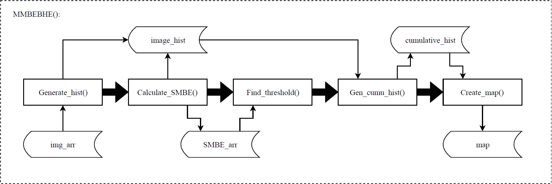
Figure 1: FPGA implementation flowchart

IV Implementation on FPGA

Following are the details of how MMBEBHE was implemented on Basys 3. The algorithm was broken down into logical modules. Each module was tested separately before being pipelined for the final result. Our implementation works on 8-bit image of arbitrary size. However, due to the complexity of the generated schematic, we have included a bare-bones schematic for a binary image with 8 pixels which is easier to comprehend.

Figure 1 shows the high-level interaction between different modules. The execution stops after the output map is calculated. Although this paper presents the implementation as different modules, the final synthesis was coalesced into a single mmbebhe module, which takes image as input and outputs the corresponding map.

IV-A Generate_hist()

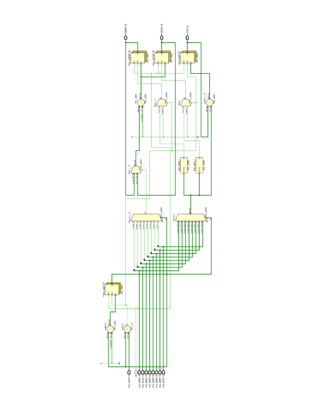
Figure 2: Generate_histogram() schematic for binary image with 8 pixels

This module takes the image as input, and outputs a histogram of frequency of each pixel value. Internally, this module contains a pointer to the image array and uses it to access one element per clock cycle. This retrieved value is used to increment the frequency in a histogram that is also kept internally, and added to a register sum, which tracks the sum of all the pixels seen. Once the module has iterated over all the pixels, a done flag is set to 1. The saved histogram is sent further down the pipe to the other modules that need it, and the execution within the module stops.

The input image array splits into two branches: one for calculating the frequency histogram freq[255], and another for calculating the sum of all pixels in the image. For calculating freq, the pixel value at index is extracted from image, and 1 is added to the register corresponding to the pixel value. For calculating sum, pixel value is extracted, and passed through an adder along with a register, sum, which stores the running sum of all seen pixels.

IV-B Calculate_smbe()

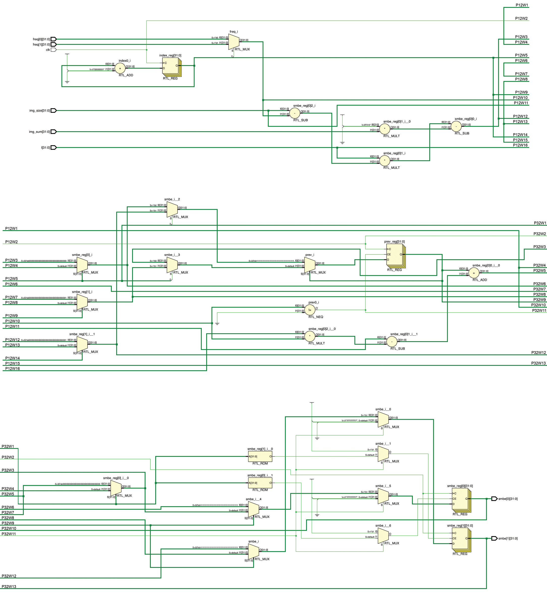
Figure 3: Calculate_SMBE() for a binary image with 8 pixels

This module is responsible for calculating the SMBE for each pixel value present in the image. For a pixel value not present in the image, the SMBE is set to 0x7fffffff, to ensure it will not be chosen as the threshold. Calculate_SMBE() takes the histogram, and sum from Generate_Hist() as input. Internally, it iterates through the histogram, and for each pixel value calculates the SMBE as described in equation (7) and (8) and stores it in a map. Note that in equation (7), $\sum^{L-1}_{i=0}{i\cdot F(X_{i})}$ is the sum of all pixels in the image. This sum is calculated by Generate_Hist() and simply consumed by this module. Once all SMBEs are calculated, a done flag is tripped to stop execution of the module and trigger the next step in the pipeline.

Since calculating SMBE values is defined recursively, with each SMBE depending on the previous one, the module uses a 32-bit register prev to store the previous entry. A register first is initialized to 0, as sentinel for the base case. The input frequency array freq goes through a multiplexer which uses index as the selector to iterate through each pixel’s frequency. The selected frequency is compared to 0. If frequency is 0, the corresponding SMBE is set to 0x7fffffff. Otherwise, the recursive formula is followed. This repeats serially for each pixel value in freq array, with prev getting updated whenever a non-zero frequency is processed. It is important to execute this part serially due to dependence on the previous element.

IV-C Find_Threshold()

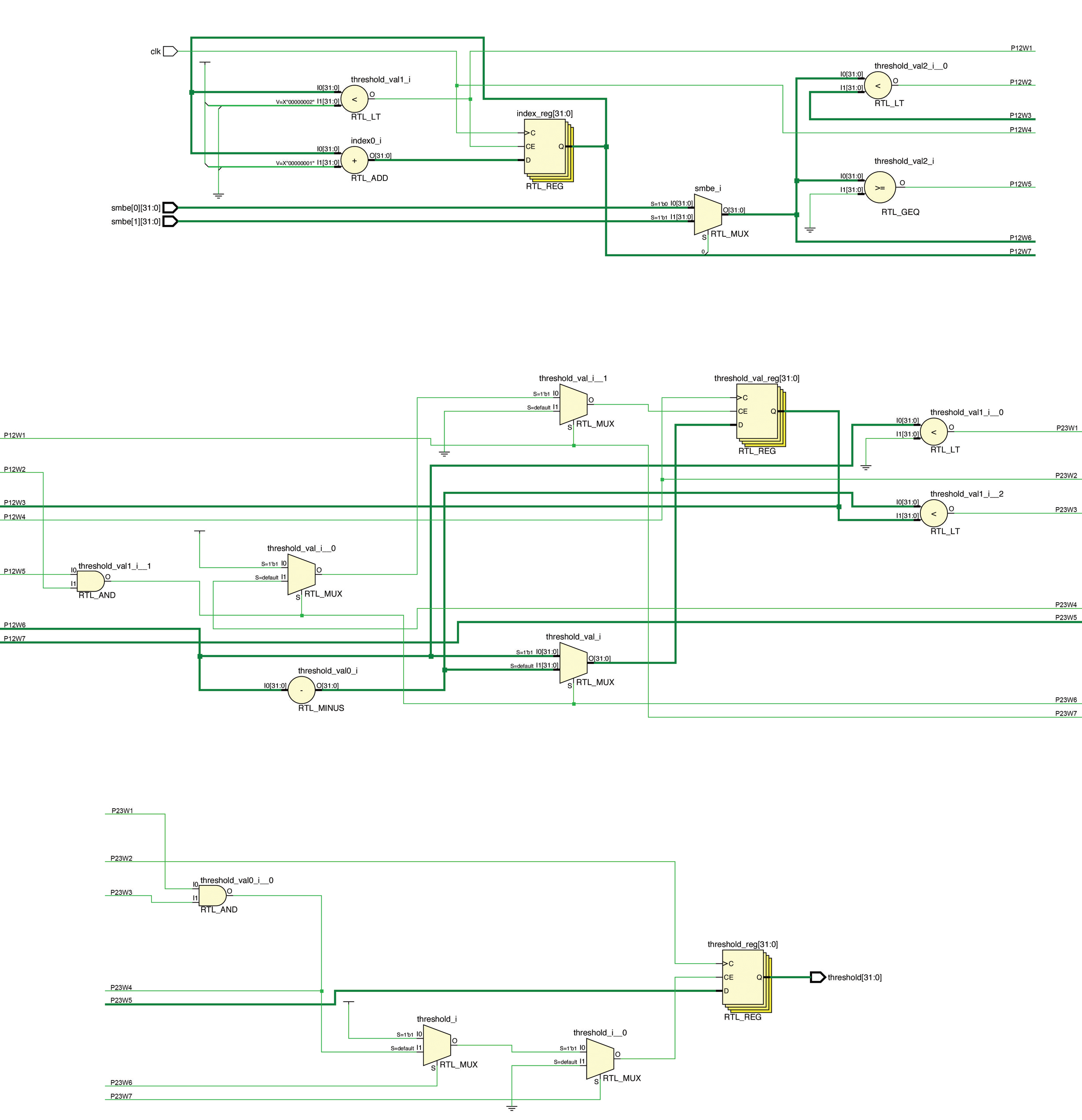
Figure 4: Find_threshold() schematic for a binary image with 8 pixels

This module takes the SMBE map from Calculate_SMBE() and looks for the pixel value which has absolute minimum SMBE. This value is the threshold along which the histogram will be divided further down the pipeline. This value is stored and passed forward along with a done flag.

The input SMBE values pass through a multiplexer with index as selector. The selected SMBE_val goes through comparators that compare the absolute value of SMBE_val to the current threshold_val. The absolute value comparison is evaluated as follows: SMBE_val < 0 && -SMBE_val < threshold_val, and SMBE_val >= 0 && SMBE_val < threshold_val. If either condition evaluates to true, threshold_val is set to SMBE_val, or -SMBE_val as appropriate, and index is saved for output. index then increments by 1, and the process repeats until index < 256.

IV-D Gen_cumu_hist()

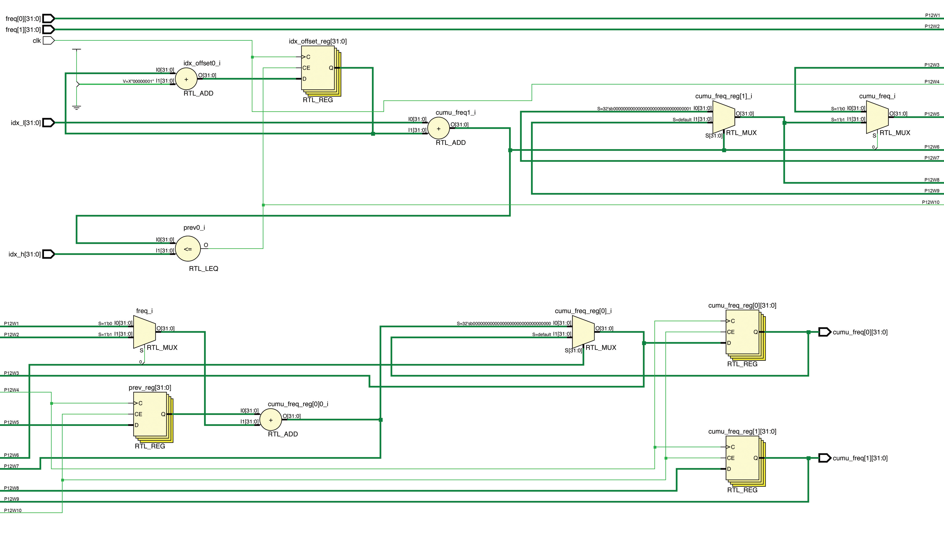
Figure 5: Gen_cumu_hist() schematic for a binary image with 8 pixels

This module takes the histogram from Generate_Hist(), a lower bound, and an upper bound and calculates the cumulative frequencies for each pixel value between the input bounds. This module is called twice by the driver module, once with bounds [0, threshold] and again with bounds [threshold+1, 255]. The cumulative frequency of each pixel value is calculated as defined in (3).

Cumulative histogram is defined as a recursive algorithm. Hence, we create a 32-bit register prev to store the last calculated value. prev is initialized to 0, for the base case. Also, since this module works within a given bound of [idx_l, idx_h], a register idx_offset is used to store index offset, instead of absolute index. The absolute index is calculated as idx_l + idx_offset. The execution does not stop until index <= idx_h evaluates to false. The input frequency array freq, passes through a multiplexer with index as selector. The selected value passes through an adder, which stores the sum of selected frequency, freq[index], and previous cumulative frequency, prev, in a separate cumu_freq array. cumu_freq is the output of this module.

IV-E Create_map()

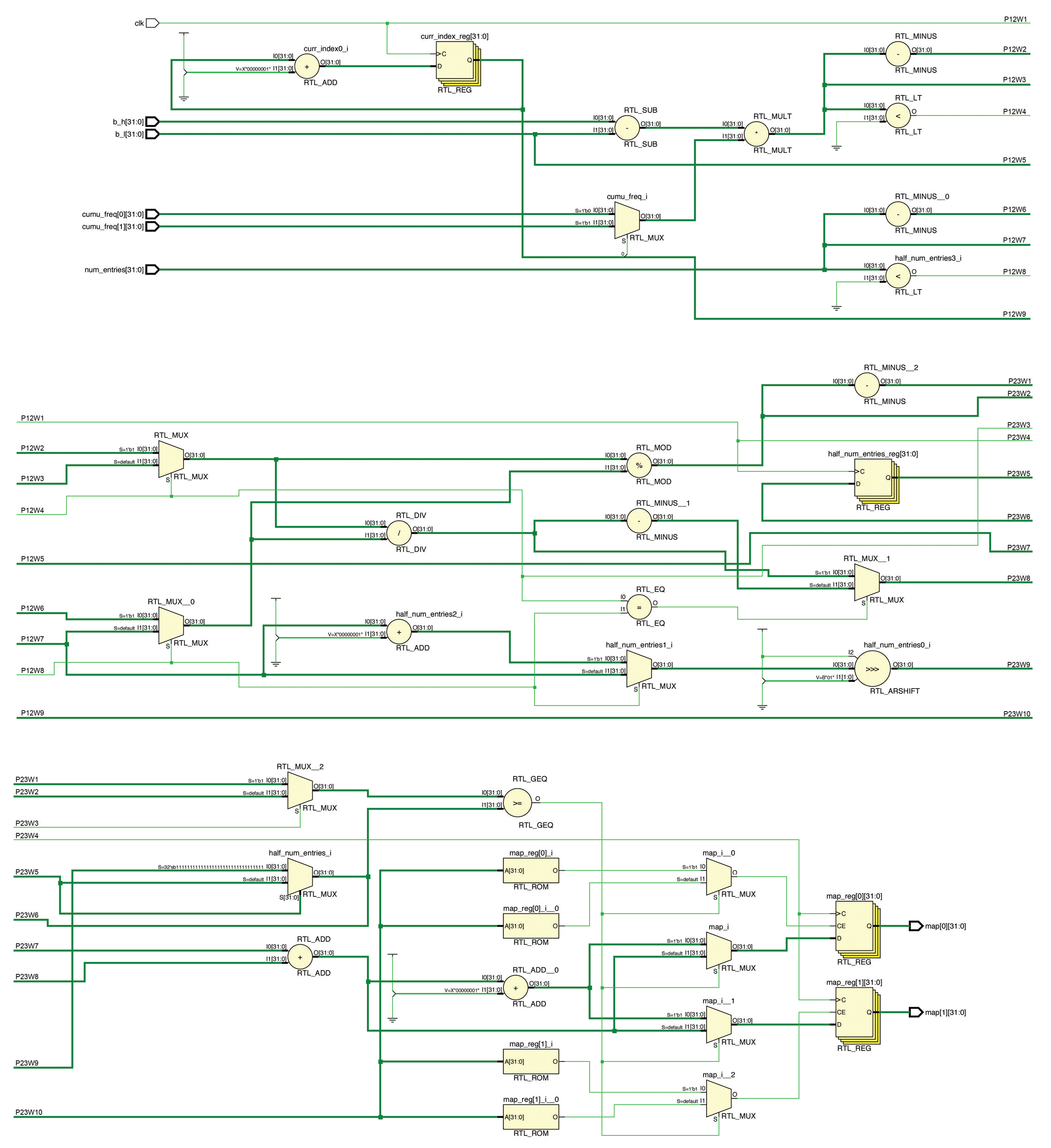
Figure 6: Create_map() schematic for a binary image with 8 pixels

This module is the last step in MMBEBHE. It creates a map between the input pixel values and output pixel values. The map is used to create the final output image. It takes the cumulative frequencies, lower bound, and upper bound as input, and outputs the map for the given bounds. Much like Gen_cumu_hist(), this module is called twice, once with bounds $[0,threshold]$ and again with bounds $[threshold+1,255]$. The map is calculated as defined in (5). Since the output is a pixel value, we use integer division, and round using modulus ($\%$) operator. The output maps are sent forward to be compiled into a single map.

Calculating map is carried out as described in (5). This process can be entirely parallelized, but we carry it out serially to reduce hardware size. When the module starts executing, we calculate the half of the total number of pixels, num_entries, in the input image. This value is calculated as a right shift, i.e., num_entries >> 1, and is stored in a 32-bit register half_num_entries. half_num_entries is used to round values up. The input cumulative frequency array cumu_freq passes through a multiplexer with a index as selector. The selected frequency is use to calculate the corresponding map value. Simultaneously, the remainder with num_entries is calculated. If the remainder is greater than half_num_entries, the map value is increased by one. This process repeats for each pixel value.

IV-F MMBEBHE()

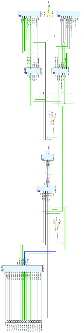
Figure 7: MMBEBHE Schematic for a binary image with 8 pixels

This is the driver module, responsible for pipelining the other modules. Figure 7 shows how the differed mmodules interact with each other. Our implementation takes image and the image size as input, and outputs a map from input pixel values to output pixel values. To get the final image, the value of each pixel is replaced with corresponding value in the output map.

V Experimental Results

The map generated by the FPGA on synthesizing our implementation matched the simulation, and result from MATLAB. The output map can be used to recreate the equalized image. Figure 8, and Figure 9 compare the original image, image created by FPGA, and image created by MATLAB. Results from MATLAB and FPGA are visually and objectively similar, as depicted by their histograms. Therefore, our implementation successfully recreates the results of MMBEBHE on an FPGA, without using floating point arithmetic.

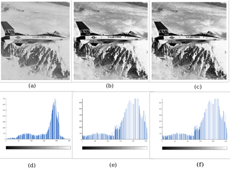
Figure 8: F16 Images Comparison

(a): Original image; (b): output from FPGA; (c): Output from MATLAB. (d),(e), & (f) are histograms of (a),(b), & (c) respectively.

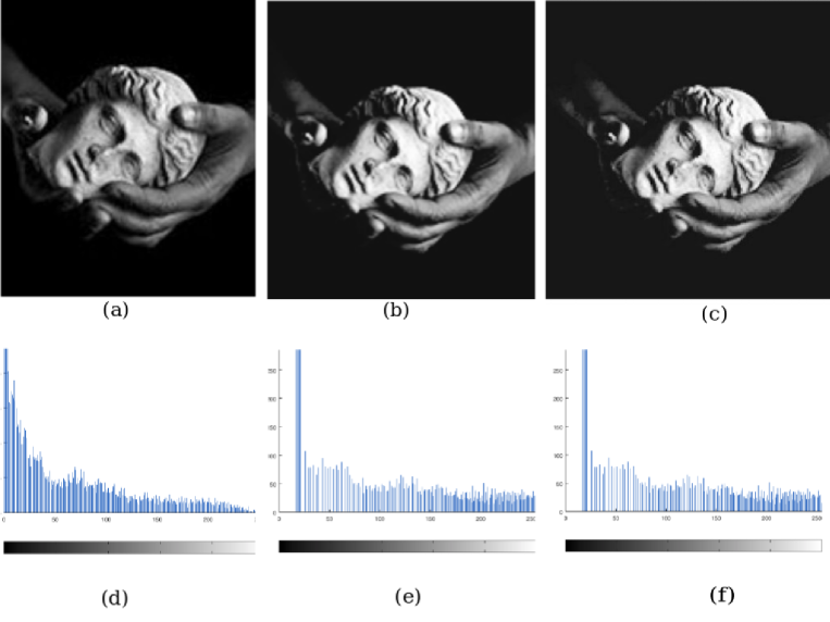
Figure 9: Hands Output Images Comparison

(a): Original image; (b): output from FPGA; (c): Output from MATLAB. (d),(e), & (f) are histograms of (a),(b), & (c) respectively.

Although timing actual execution of logic on FPGA is cumbersome, we were able to get an approximate execution time of each logical module through simulations. Table I shows comparison between execution times of each logical module in our FPGA implementation with 300 MHz clock, and floating point MATLAB implementation.

TABLE I: Timings of MMBEBHE on F16 Image — FPGA vs MATLAB

Module	FPGA Simulation Timing (300 MHz clock) (in $\mu$s)	MATLAB Timing (in $\mu$s)
Generate_hist()	207.68	268
Calculate_SMBE()	2.57	31
Find_Threshold()	2.57	12
Gen_Cumu_Hist()	2.6	78
Create_Map()	2.6

Table III, and Table IV show the utilization report of our implementation. Compare this to the resource utilization report of Histogram Equalization as computed by Sawmya and Paily[9], in Table II.

TABLE II: Resource Utilization of Histogram Equalization by Sowmya and Paily[9]

Device	xc2vp30-7ff896
I/O Cells	32 of 556 (5%)
Block RAMs	16 of 136(11%)
Time Period	5ns
Power	148mW

TABLE III: DSP Utilization table

Site Type	Used	Available	Util%
DSPs	6	90	6.67

TABLE IV: Slice Logic Utilization table

Site Type	Used	Available	Util%
1) Slice LUTs	6923	20800	33.28
a) LUT as logic	6315	20800	30.36
b) LUT as memory	608	9600	6.33
2) Slice Registers	952	41600	2.29
a) Registers as Flip Flop	929	41600	2.23
b) Registers as Latch	23	41600	0.06
3) F7 Muxes	1916	16300	11.75
4) F8 Muxes	525	8150	6.44

VI Conclusions and Future Work

We present a successful implementation of MMBEBHE on FPGA. We are able to replicate the results of MMBEBHE as found in MATLAB and ModelSim simulations on our FPGA. The future work could potentially include performing the MMBEBHE on larger images, as well as optimizing it to increase parallel processing and hardware concurrency.

References

- [1] J. Zimmerman, S. Pizer, E. Staab, E. Perry, W. McCartney, B. Brenton, “Evaluation of the effectiveness of adaptive histogram equalization for contrast enhancement,” IEEE Trans. on Medical Imaging, pp. 304-312, Dec. 1988.
- [2] Y. Li, W. Wang, D. Y. Yu, “Application of adaptive histogram equalization to x-ray chest image,” Proc. of the SPIE, vol. 2321, pp. 513-514, 1994.
- [3] Yeong-Taeg Kim, “Method and circuit for video enhancement based on the mean separate histogram equalization,”filed in a Korean patent, March 9, 1996, Appl. No. 6219.
- [4] Y. T. Kim, “Contrast enhancement using brightness preserving bi-histogram equalization,” IEEE Trans. Consum. Electron., vol. 43, no. 1, pp. 1–8, Feb. 1997.
- [5] Chen and A. Ramli, “Minimum mean brightness error bi- histogram equalization in contrast enhancement,” IEEE Trans. Consum.Electron., pp. 1310–1319 Nov. 2003.
- [6] A. Trost, B. Zajc Zemva, ”Pogrammable System for Image Processing” in Field-Programmable Logic and Applications, Elsevier, pp. 490-494, 1998.
- [7] Wang Bing-jian, Liu Shang-qian, Qing Li, Zhou Hui-xin, ”A realtime contrast enhancement algorithm for infrared images based on plateau histogram”, Infrared Physics and Technology Elsevier, pp. 77-82, 2006.
- [8] Abduallah M. Alsuwailem, Saleh A. Alshebeili, ”A New approach for real-time histogram equalization using FPGA”, Proceedings of International Symposium on Intelligent Signal Processing and Communication Systems, 2005.
- [9] S. Sowmya and R. Paily, “FPGA implementation of image enhancement algorithms,” 2011 International Conference on Communications and Signal Processing, Calicut, 2011, pp. 584-588.