MADAN: Multi-source Adversarial Domain Aggregation Network for Domain Adaptation

Abstract

Domain adaptation aims to learn a transferable model to bridge the domain shift between one labeled source domain and another sparsely labeled or unlabeled target domain. Since the labeled data may be collected from multiple sources, multi-source domain adaptation (MDA) has attracted increasing attention. Recent MDA methods do not consider the pixel-level alignment between sources and target or the misalignment across different sources. In this paper, we propose a novel MDA framework to address these challenges. Specifically, we design an end-to-end Multi-source Adversarial Domain Aggregation Network (MADAN). First, an adapted domain is generated for each source with dynamic semantic consistency while aligning towards the target at the pixel-level cycle-consistently. Second, sub-domain aggregation discriminator and cross-domain cycle discriminator are proposed to make different adapted domains more closely aggregated. Finally, feature-level alignment is performed between the aggregated domain and the target domain while training the task network. For the segmentation adaptation, we further enforce category-level alignment and incorporate context-aware generation, which constitutes MADAN+. We conduct extensive MDA experiments on digit recognition, object classification, and simulation-to-real semantic segmentation. The results demonstrate that the proposed MADAN and MANDA+ models outperform state-of-the-art approaches by a large margin.

1 Introduction

Together with increased computation capacity and deep complex models, large-scale labeled data attributes to the significant success of deep learning algorithms as one key element. Consequently, promising performance has been obtained via deep neural networks in various computer vision tasks, such as image classification [1, 2, 3, 4], object detection [5, 6, 7], and semantic segmentation [8, 9, 10]. However, in many real-world applications, there are only limited or even no labeled training data, as labeling is expensive, time-consuming, and difficult. For example, only the labels provided by experts are reliable in fine-grained recognition [11]; labeling each Cityscapes image takes about 90 minutes in semantic segmentation [12]; point-wise 3D LiDAR point clouds are difficult to label in autonomous driving [13, 14]. One direct way is to transfer the learned knowledge from one labeled source domain to another different but related target domain. However, because of the presence of domain shift or dataset bias [15], i.e. the joint probability distributions of observed data and labels are different in the two domains, direct transfer may not perform well, as shown in Figure 1. This observation motivates the research on domain adaptation (DA) [16, 17].

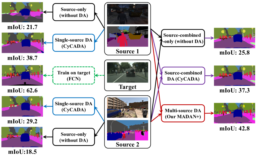
Figure 1: An example of domain shift. Source 1: GTA, Source 2: SYNTHIA, Target: Cityscapes. Left three columns: single-source DA. The overall mIoU result of the FCN semantic segmentation model [8] drops from 62.6% (trained on the target Cityscapes, unavailable in UDA and simply used for comparison here) to 21.7% and 18.5% (trained only on the source GTA and SYNTHIA). CyCADA achieves 38.7% and 29.2%, demonstrating that DA can bridge the domain gap. Right three columns: multi-source DA. Simply combining multiple sources and performing single-source DA (37.3%) does not outperform the best single-source DA (38.7%). We propose Multi-source Adversarial Domain Aggregation Network (MADAN), a novel adversarial model, to perform multi-source DA. Our method achieves significant performance improvements over source-combined DA, source-combined only, and single-source DA.

Without requiring any labeled data from the target domain, unsupervised domain adaptation (UDA) is the most widely studied pipeline. Both theoretical analysis [18, 19, 20, 17] and algorithm design [21, 22, 23, 24, 25, 26, 27, 28] for UDA have been proposed recently. Conventional UDA methods mainly focus on the single-source scenario based on the assumption that the labeled source data is sampled from the same distribution. However, in practice, the labeled data may be collected from multiple sources with different distributions [29, 30]. Simply combining different sources into one source and directly employing single-source UDA may lead to suboptimal solutions, since the data from different sources may interfere with each other during the learning process [31], as shown in Figure 1. Therefore, effective multi-source domain adaptation (MDA) algorithms are required.

Early efforts on MDA mainly used shallow models [29], either learning a latent feature space for different domains [32, 33, 34, 35, 36] or combining pre-learned source classifiers [37, 38, 39, 40]. Recently, some deep MDA methods that only focus on image classification have been proposed by learning a common feature space and aligning each source and target pair [41, 42, 43, 30]. There are some limitations of these methods. (1) They mainly focus on feature-level alignment, which only aligns high-level information. This might be sufficient for coarse-grained classification tasks, but it is obviously insufficient for fine-grained semantic segmentation, which performs pixel-wise prediction. Further, they have low interpretability, which cannot well explain why these methods work. (2) They only align each source and target pair. Although different sources are matched towards the target, there may exist significant mis-alignment across different sources. (3) They only focus on image classification where one label is assigned to each image. Directly extending them from classification to segmentation, which assigns a semantic label (e.g. car, cyclist, pedestrian, road) to each pixel in an image, may not perform well. This is because segmentation is a structured prediction task, i.e. it has to resolve the predictions in an exponentially large label space and thus the decision function is more involved than classification [44, 45].

To address the above challenges, in this paper we propose a novel MDA framework, termed Multi-source Adversarial Domain Aggregation Network (MADAN), which consists of Dynamic Adversarial Image Generation, Adversarial Domain Aggregation, and Feature-aligned task learning. First, for each source, we generate an adapted domain using a Generative Adversarial Network (GAN) [46] with cycle-consistency constraint [47], which enforces pixel-level alignment between source images and target images. To preserve the semantics before and after image translation, we propose a novel semantic consistency loss by minimizing the Kullback–Leibler (KL) divergence between the source predictions of a pretrained task model (e.g. classification and segmentation) and the adapted predictions of a dynamic task model. Second, instead of training a classifier for each source domain [41, 43, 30], we propose sub-domain aggregation discriminator to directly make different adapted domains indistinguishable, and cross-domain cycle discriminator to discriminate between the images from each source and the images transferred from other sources. In this way, different adapted domains can be better aggregated into a more unified domain. Finally, the task model is trained on the aggregated domain, while enforcing feature-level alignment between the aggregated domain and the target domain.

In summary, our contributions are three-fold:

• We design a novel framework termed MADAN to do multi-source domain adaptation. (i) Sub-domain aggregation discriminator and cross-domain cycle discriminator are proposed to better align different adapted domains. (ii) Besides feature-level alignment, pixel-level alignment is further considered by generating an adapted domain for each source cycle-consistently with a novel dynamic semantic consistency loss.

• We propose to perform domain adaptation for semantic segmentation from multiple sources. To our best knowledge, this is the first work on multi-source structured domain adaptation. For segmentation, MADAN is enhanced to MADAN+ with category-level alignment and context-aware generation.

• We conduct extensive experiments on several MDA bechmark datasets for digit recognition, object classification, and simulation-to-real semantic segmentation, and the results demonstrate the effectiveness of the proposed MADAN and MADAN+ models.

One preliminary version on MADAN was previously introduced in our NeurIPS conference paper [48]. As compared to the conference version, this journal paper has the following three aspects of enhancements. First, we perform a more comprehensive review to compare the proposed method with existing methods. Second, we conduct MDA experiments on digit recognition and object classification, which also achieves state-of-the-art performances, and enrich the analysis of the results. Third, we extend the original MADAN to MADAN+ with category-level alignment and context-aware generation for semantic segmentation, conduct more comparative experiments, and achieve better performances.

The rest of this paper is organized as follows. Section 2 reviews related work on single-source UDA and MDA. Section 3 gives the definition of the MDA problem. Section 4 describes the proposed MADAN and extended MADAN+ models in detail. Experimental settings, results, and analysis are presented in Section 5. We conclude this paper in Section 6.

Table I: Comparison of the proposed MADAN model with several state-of-the-art domain adaptation methods. The full names of each property from the third to the last columns are pixel-level alignment, context-aware generation, feature-level alignment, category-level alignment, semantic consistency, cycle consistency, multiple sources, domain aggregation, one task network, fine-grained prediction, and end-to-end training, respectively.

DA setting

method

pixel

con

feat

cat

sem

cycle

multi

aggr

one

fine

end

ADDA [17]

✗

✗

✓

✗

–

–

✗

–

✓

✓

✗

CycleGAN [47]

✓

✗

✗

✗

✗

✓

✗

–

✓

✗

✗

PixelDA [49]

✓

✗

✗

✗

✗

✗

✗

–

✓

✓

✓

NMD [50]

✗

✗

✓

✓

-

-

✗

–

✓

✓

✓

single-source

SBADA [51]

✓

✗

✗

✗

✓

✓

✗

–

✓

✗

✓

GTA-GAN [52]

✓

✗

✓

✗

✗

✗

✗

–

✓

✗

✓

DupGAN [53]

✓

✗

✓

✗

✓

✗

✗

–

✓

✗

✓

CyCADA [27]

✓

✗

✓

✗

✓

✓

✗

–

✓

✓

✓

DCTN [41]

✗

✗

✓

✗

–

–

✓

✗

✗

✗

✓

MDAN [42]

✗

✗

✓

✗

–

–

✓

✗

✓

✗

✓

multi-source

MMN [43]

✗

✗

✓

✗

–

–

✓

✗

✗

✗

✓

MDDA [30]

✗

✗

✓

✗

–

–

✓

✗

✗

✗

✗

MADAN (ours)

✓

✗

✓

✗

✓

✓

✓

✓

✓

✓

✓

MADAN+ (ours)

✓

✓

✓

✓

✓

✓

✓

✓

✓

✓

✓

2 Related Work

In this section, we introduce related work on single-source unsupervised domain adaptation and multi-source domain adaptation, and compare the proposed MADAN with these methods.

2.1 Single-source UDA

While the early single-source UDA (SUDA) methods are mainly non-deep ones [54], either re-weighting samples or transforming intermediate subspaces, the emphasis of recent SUDA methods has shifted to deep learning architectures in an end-to-end fashion. Typically, a conjoined architecture with two streams is employed in deep SUDA [55]. One stream is used to represent the task model for the source domain, and the other is used to align the target and source domains. Correspondingly, a traditional task loss based on the labeled source data and another alignment loss to tackle the domain shift problem are jointly optimized during the training of deep SUDA. Typically, the task loss is the same among different methods, while the difference is focused on the alignment loss, such as discrepancy loss, adversarial loss, reconstruction loss, etc.

Discrepancy-based methods explicitly measure the discrepancy between the target domain and the source domain, such as the multiple kernel variant of maximum mean discrepancies [26], correlation alignment (CORAL) [56, 55], geodesic distance [13], and contrastive domain discrepancy [57]. Adversarial generative methods combine the domain discriminative model with a generative component to generate fake source or target data generally based on GAN [46, 49] and its variants, such as CoGAN [58], SimGAN [59], CycleGAN [47, 28, 60], and CyCADA [27]. Adversarial discriminative methods usually employ an adversarial objective with respect to a domain discriminator to encourage domain confusion [61, 17, 50, 62, 45, 63]. Reconstruction based methods try to reconstruct the target input from the features extracted using the source task model by minimizing the reconstruction loss [25, 64]. While the adversarial generative methods consider the pixel-level alignment, the others mainly employ feature-level alignment. Although these methods make remarkable progress to SUDA, they suffer from large performance decay when directly applied to the MDA problem.

2.2 Multi-source Domain Adaptation

Multi-source domain adaptation (MDA) considers a more practical scenario, where the training data are collected from multiple sources [29, 48]. Some theoretical analysis [18, 65] is developed to support existing MDA algorithms. The early MDA methods mainly focus on shallow models, including two categories [29]: feature representation approaches [32, 33, 34, 35, 36] and combination of pre-learned classifiers [37, 38, 39, 40]. Some recent shallow MDA methods mainly aim to deal with special cases, such as incomplete MDA [66] and target shift [67].

Recently, some representative deep learning based MDA methods are proposed, such as multisource domain adversarial network (MDAN) [42], deep cocktail network (DCTN) [41], moment matching network (MMN) [43], and multi-source distilling domain adaptatioin (MDDA) [30]. All these MDA methods only consider the feature-level alignment for image classification tasks. The former three methods employ a shared feature extractor to symmetrically map the multiple sources and target into the same space. For each source-target pair in MDAN and DCTN, a discriminator is trained to distinguish the source and target features. MDAN directly concatenates all extracted source features and labels into one domain and train a single task model, while a task model is trained for each source domain in DCTN, which combines the predictions of different models for a target image using perplexity scores as weights. MMN transfers the learned knowledge from multiple sources to the target by dynamically aligning moments of their feature distributions. The final prediction of a target image is averaged uniformly based on the classifiers from different source domains. MDDA first pre-trains a feature extractor for each source and match the target feature to each source feature space asymmetrically. After distilling the pre-trained classifiers with selected representative samples in each source, the predictions of the matched target features using corresponding source classifiers are combined based on the weights obtained from the Wasserstein distance. Differently, we also consider the pixel-level alignment. Based on the aggregated intermediate domain obtained by sub-domain aggregation discriminator and cross-domain cycle discriminator, only one task model needs to be trained. Besides the image classification tasks, we also perform semantic segmentation task, which is the first work on MDA for segmentation. Table I compares MADAN with several state-of-the-art DA methods.

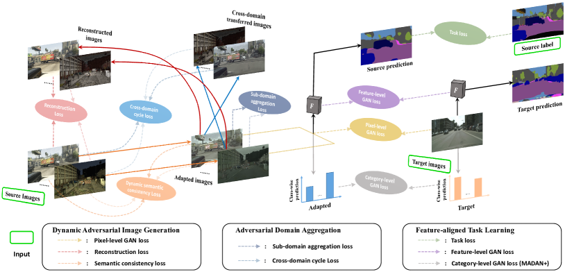
Figure 2: The framework of the proposed Multi-source Adversarial Domain Aggregation Network (MADAN). The colored solid arrows represent generators, while the black and grey solid arrows indicate the task network $F$. The dashed arrows correspond to different losses.

3 Problem Setup

We consider the unsupervised MDA scenario with multiple labeled source domains $S_{1},S_{2},\cdots,S_{M}$, where $M$ is number of sources, and one unlabeled target domain $T$. In the $i$th source domain $S_{i}$, suppose $X_{i}=\{\mathbf{x}_{i}^{j}\}_{j=1}^{N_{i}}$ and $Y_{i}=\{\mathbf{y}_{i}^{j}\}_{j=1}^{N_{i}}$ are the observed data and corresponding labels drawn from the source distribution $p_{i}(\mathbf{x},\mathbf{y})$, where $N_{i}$ is the number of samples in $S_{i}$. For different tasks, the format of labels $\mathbf{y}_{i}^{j}$ varies. For example, in classification, each image has a unique $\mathbf{y}_{i}^{j}$; in segmentation, $\mathbf{y}_{i}^{j}$ is pixel-wise. In the target domain $T$, let $X_{T}=\{\mathbf{x}_{T}^{j}\}_{j=1}^{N_{T}}$ denote the target data drawn from the target distribution $p_{T}(\mathbf{x},\mathbf{y})$ without label observation, where $N_{T}$ is the number of target samples. Unless otherwise specified, we have two assumptions: (1) homogeneity, i.e. $\mathbf{x}_{i}^{j}\in\mathbb{R}^{d},\mathbf{x}_{T}^{j}\in\mathbb{R}^{d}$, indicating that the data from different domains are observed in the same image space but with different distributions; (2) closed set, i.e. $\mathbf{y}_{i}^{j}\in\mathcal{Y},\mathbf{y}_{T}^{j}\in\mathcal{Y}$, where $\mathcal{Y}$ is the label set, which means that all the domains share the same space of classes. Based on covariate shift and concept drift [54], we aim to learn an adaptation model that can correctly predict the labels of a sample from the target domain trained on $\{(X_{i},Y_{i})\}_{i=1}^{M}$ and $\{X_{T}\}$. How to extend the unsupervised, homogeneous, and closed set MDA method to other settings, such as heterogeneous DA, open set DA, and category-shift DA remains our future work.

4 Multi-source Adversarial Domain Aggregation Network

In this section, we introduce the proposed Multi-source Adversarial Domain Aggregation Network (MADAN) for image classification and semantic segmentation adaptation in detail. The framework is illustrated in Figure 2, which consists of three components: Dynamic Adversarial Image Generation (DAIG), Adversarial Domain Aggregation (ADA), and Feature-aligned Task Learning (FTL). DAIG aims to generate adapted images from source domains to the target domain from the perspective of visual appearance while preserving the semantic information dynamically. In order to reduce the distances among the adapted domains and thus generate a more aggregated unified domain, ADA is proposed, including Cross-domain Cycle Discriminator (CCD) and Sub-domain Aggregation Discriminator (SAD). Finally, FTL learns the domain-invariant representations at the feature-level in an adversarial manner.

4.1 Dynamic Adversarial Image Generation

The goal of DAIG is to make images from different source domains visually similar to the target images, as if they are drawn from the same target domain distribution. To this end, for each source domain $S_{i}$, we introduce a generator $G_{S_{i}\rightarrow T}$ mapping to the target $T$ in order to generate adapted images that fool $D_{T}$, which is a pixel-level adversarial discriminator. $D_{T}$ is trained simultaneously with each $G_{S_{i}\rightarrow T}$ to classify real target images $X_{T}$ from adapted images $G_{S_{i}\rightarrow T}(X_{i})$. The corresponding GAN loss function is:

$$\mathcal{L}_{GAN}^{S_{i}\rightarrow T}(G_{S_{i}\rightarrow T},D_{T},X_{i},X_{T})=$$ (1)

$$\mathbb{E}_{\mathbf{x}_{i}\sim X_{i}}\log D_{T}(G_{S_{i}\rightarrow T}(\mathbf{x}_{i}))+\mathbb{E}_{\mathbf{x}_{T}\sim X_{T}}\log[1-D_{T}(\mathbf{x}_{T})].$$

Since the mapping $G_{S_{i}\rightarrow T}$ is highly under-constrained [46], we employ an inverse mapping $G_{T\rightarrow S_{i}}$ as well as a cycle-consistency loss [47] to enforce $G_{T\rightarrow S_{i}}(G_{S_{i}\rightarrow T}(\mathbf{x}_{i}))\approx\mathbf{x}$ and vice versa. Similarly, we introduce $D_{i}$ to classify $X_{i}$ from $G_{T\rightarrow S_{i}}(X_{T})$, with the following GAN loss:

$$\mathcal{L}_{GAN}^{T\rightarrow S_{i}}(G_{T\rightarrow S_{i}},D_{i},X_{T},X_{i})=$$ (2)

$$\mathbb{E}_{\mathbf{x}_{i}\sim X_{i}}\log[1-D_{i}(\mathbf{x}_{i})]+\mathbb{E}_{\mathbf{x}_{T}\sim X_{T}}\log D_{i}(G_{T\rightarrow S_{i}}(\mathbf{x}_{T})).$$

The cycle-consistency loss [47] ensures that the learned mappings $G_{S_{i}\rightarrow T}$ and $G_{T\rightarrow S_{i}}$ are cycle-consistent, thereby preventing them from contradicting each other, is defined as:

$$\mathcal{L}_{cyc}^{S_{i}\leftrightarrow T}(G_{S_{i}\rightarrow T},G_{T\rightarrow S_{i}},X_{i},X_{T})=$$ (3)

$$\mathbb{E}_{\mathbf{x}_{i}\sim X_{i}}\parallel G_{T\rightarrow S_{i}}(G_{S_{i}\rightarrow T}(\mathbf{x}_{i}))-\mathbf{x}_{i}\parallel_{1}+$$

$$\mathbb{E}_{\mathbf{x}_{T}\sim X_{T}}\parallel G_{S_{i}\rightarrow T}(G_{T\rightarrow S_{i}}(\mathbf{x}_{T}))-\mathbf{x}_{T}\parallel_{1}.$$

The adapted images are expected to contain the same semantic information as original source images, but the semantic consistency is only partially constrained by the cycle consistency loss. The semantic consistency loss in CyCADA [27] was proposed to better preserve semantic information. $\mathbf{x}_{i}$ and $G_{S_{i}\rightarrow T}(\mathbf{x}_{i})$ are both fed into a task model $F_{i}$ pretrained on $(X_{i},Y_{i})$. However, since $\mathbf{x}_{i}$ and $G_{S_{i}\rightarrow T}(\mathbf{x}_{i})$ are from different domains, employing the same task model, i.e. $F_{i}$, to obtain the predicted results and then computing the semantic consistency loss may be detrimental to image generation. Ideally, the adapted images $G_{S_{i}\rightarrow T}(\mathbf{x}_{i})$ should be fed into a network $F_{T}$ trained on the target domain, which is infeasible since target domain labels are not available in UDA. Instead of employing $F_{i}$ on $G_{S_{i}\rightarrow T}(\mathbf{x}_{i})$, we propose to dynamically update the network $F_{A}$, which takes $G_{S_{i}\rightarrow T}(\mathbf{x}_{i})$ as input, so that its optimal input domain (the domain that the network performs best on) gradually changes from that of $F_{i}$ to $F_{T}$. We employ the task model $F$ trained on the adapted domain as $F_{A}$, i.e. $F_{A}=F$, which has two advantages: (1) $G_{S_{i}\rightarrow T}(\mathbf{x}_{i})$ becomes the optimal input domain of $F_{A}$, and as $F$ is trained to have better performance on the target domain, the semantic loss after $F_{A}$ would promote $G_{S_{i}\rightarrow T}$ to generate images that are closer to target domain at the pixel-level; (2) since $F_{A}$ and $F$ can share the parameters, no additional training or memory space is introduced, which is quite efficient. The proposed dynamic semantic consistency (DSC) loss is:

$$\mathcal{L}_{DSC}^{S_{i}}(G_{S_{i}\rightarrow T},X_{i},F_{i},F_{A})=$$ (4)

$$\mathbb{E}_{\mathbf{x}_{i}\sim X_{i}}KL(F_{A}(G_{S_{i}\rightarrow T}(\mathbf{x}_{i}))||F_{i}(\mathbf{x}_{i})),$$

where $KL(\cdot||\cdot)$ is the KL divergence between two distributions.

4.2 Adversarial Domain Aggregation

We can train different task models for each adapted domain and combine different predictions with specific weights for target images [41, 43], or we can simply combine all adapted domains together and train one model [42]. In the first strategy, it is challenging to determine how to select the weights for different adapted domains. Moreover, each target image needs to be fed into all task models at reference time, and this is rather inefficient. For the second strategy, since the alignment space is high-dimensional, although the adapted domains are relatively aligned with the target, they may be significantly misaligned with each other. In order to mitigate this issue, we propose adversarial domain aggregation to make different adapted domains more closely aggregated with two kinds of discriminators. One is the sub-domain aggregation discriminator (SAD), which is designed to directly make the different adapted domains indistinguishable. For $S_{i}$, a discriminator $D_{A}^{i}$ is introduced with the following loss function:

$$\mathcal{L}_{SAD}^{S_{i}}(G_{S_{1}\rightarrow T},\dots G_{S_{i}\rightarrow T},\dots,G_{S_{M}\rightarrow T},D_{A}^{i})=$$ (5)

$$\mathbb{E}_{\mathbf{x}_{i}\sim X_{i}}\log D_{A}^{i}(G_{S_{i}\rightarrow T}(\mathbf{x}_{i}))+$$

$$\frac{1}{M-1}\sum\nolimits_{j\neq i}\mathbb{E}_{\mathbf{x}_{j}\sim{X_{j}}}\log[1-D_{A}^{i}(G_{S_{j}\rightarrow T}(\mathbf{x}_{j}))].$$

The other is the cross-domain cycle discriminator (CCD). For each source domain $S_{i}$, we transfer the images from the adapted domains $G_{S_{j}\rightarrow T}(X_{j}),\ j=1,\cdots,M,j\neq i$ back to $S_{i}$ using $G_{T\rightarrow S_{i}}$ and employ the discriminator $D_{i}$ to classify $X_{i}$ from $G_{T\rightarrow S_{i}}(G_{S_{j}\rightarrow T}(X_{j}))$, which corresponds to the following loss function:

$$\mathcal{L}_{CCD}^{S_{i}}(G_{T\rightarrow S_{1}},\dots G_{T\rightarrow S_{i-1}},G_{T\rightarrow S_{i+1}},\dots,G_{T\rightarrow S_{M}},G_{S_{i}\rightarrow T},D_{i})$$ (6)

$$=\mathbb{E}_{\mathbf{x}_{i}\sim X_{i}}\log D_{i}(\mathbf{x}_{i})+$$

$$\frac{1}{M-1}\sum\nolimits_{j\neq i}\mathbb{E}_{\mathbf{x}_{j}\sim X_{j}}\log[1-D_{i}(G_{T\rightarrow S_{i}}((G_{S_{j}\rightarrow T}(\mathbf{x}_{j})))].$$

Please note that using a more sophisticated combination of different discriminators’ losses to better aggregate the domains with larger distances might improve the performance. We leave this as future work and would explore this direction by dynamic weighting of the loss terms and incorporating some prior domain knowledge of the sources.

4.3 Feature-aligned Task Learning

After adversarial domain aggregation, the adapted images of different domains $X_{i}^{\prime}(i=1,\cdots,M)$ are more closely aggregated and aligned. Meanwhile, the semantic consistency loss in dynamic adversarial image generation ensures that the semantic information, i.e. the labels, is preserved before and after image translation. Suppose the images of the unified aggregated domain are $X^{\prime}=\bigcup\limits_{i=1}^{M}X_{i}^{\prime}$ and corresponding labels are $Y=\bigcup\limits_{i=1}^{M}Y_{i}$. We can then train a task learning model $F$ based on $X^{\prime}$ and $Y$. For classification and segmentation, $F$ aims to respectively minimize the following cross-entropy loss $\mathcal{L}_{task}(F,X^{\prime},Y)$:

$$\small\mathcal{L}_{cla}(F,X^{\prime},Y)=-\mathbb{E}_{(\mathbf{x}^{\prime},y)\sim(X^{{}^{\prime}},Y)}\sum\nolimits_{l=1}^{L}\mathds{1}_{[l=y]}\log(\sigma(F(\mathbf{x}^{\prime}))),\\$$ (7)

$$\mathcal{L}_{seg}(F,X^{\prime},Y)=-\mathbb{E}_{(\mathbf{x}^{\prime},\mathbf{y})\sim(X^{{}^{\prime}},Y)}\sum\nolimits_{l=1}^{L}\sum\nolimits_{h=1}^{H}\sum\nolimits_{w=1}^{W}$$ (8)

$$\mathds{1}_{[l=\mathbf{y}_{h,w}]}\log(\sigma(F_{l,h,w}(\mathbf{x}^{\prime}))),$$

where $L$ is the number of classes, $H,W$ are the height and width of the adapted images, $\sigma$ is the softmax function, $\mathds{1}$ is an indicator function, and $F_{l,h,w}(\mathbf{x}^{\prime})$ is the value of $F(\mathbf{x}^{\prime})$ at index $(l,h,w)$.

Further, we impose feature-level alignment between $X^{\prime}$ and $X_{T}$, which can improve the task performance during inference of $X_{T}$ on the task model $F$. We introduce a discriminator $D_{F}$ to achieve this goal. The GAN loss of feature-level alignment (FLA) is defined as:

$$\mathcal{L}_{FLA}(F_{f},D_{F_{f}},X^{\prime},X_{T})=$$ (9)

$$\mathbb{E}_{\mathbf{x}^{\prime}\sim X^{\prime}}\log D_{F_{f}}(F_{f}(\mathbf{x}^{\prime}))+\mathbb{E}_{\mathbf{x}_{T}\sim X_{T}}\log[1-D_{F_{f}}(F_{f}(\mathbf{x}_{T}))],$$

where $F_{f}(\cdot)$ is the output of the last convolution layer (i.e. a feature map) of the encoder in $F$.

4.4 MADAN Learning

The proposed MADAN learning framework utilizes adaptation techniques including pixel-level alignment, cycle-consistency, dynamic semantic consistency, domain aggregation, and feature-level alignment. Combining all these components, the overall objective loss function of MADAN is:

$$\mathcal{L}_{MADAN}(G_{S_{1}\rightarrow T}\cdots G_{S_{M}\rightarrow T},G_{T\rightarrow S_{1}}\cdots G_{T\rightarrow S_{M}},D_{1}\cdots D_{M},$$ (10)

$$D_{T},D_{A}^{1}\cdots D_{A}^{M},D_{F_{f}},F)=$$

$$\sum_{i=1}^{M}\Big{[}\mathcal{L}_{GAN}^{S_{i}\rightarrow T}(G_{S_{i}\rightarrow T},D_{T},X_{i},X_{T})+\mathcal{L}_{GAN}^{T\rightarrow S_{i}}(G_{T\rightarrow S_{i}},D_{i},X_{T},X_{i})$$

$$+\mathcal{L}_{cyc}^{S_{i}\leftrightarrow T}(G_{S_{i}\rightarrow T},G_{T\rightarrow S_{i}},X_{i},X_{T})+\mathcal{L}_{DSC}^{S_{i}}(G_{S_{i}\rightarrow T},X_{i},F_{i},F)$$

$$+\mathcal{L}_{SAD}^{S_{i}}(G_{S_{1}\rightarrow T},\dots G_{S_{i}\rightarrow T},\dots,G_{S_{M}\rightarrow T},D_{A}^{i})$$

$$+\mathcal{L}_{CCD}^{S_{i}}(G_{T\rightarrow S_{1}},\dots G_{T\rightarrow S_{i-1}},G_{T\rightarrow S_{i+1}},\dots,G_{T\rightarrow S_{M}},G_{S_{i}\rightarrow T},D_{i})\Big{]}$$

$$+\mathcal{L}_{task}(F,X^{\prime},Y)+\mathcal{L}_{FLA}(F_{f},D_{F_{f}},X^{\prime},X_{T}).$$

The training process corresponds to solving for a target model $F$ according to the optimization:

$$F^{*}=\arg\min_{F}\min_{D}\max_{G}\mathcal{L}_{MADAN}(G,D,F),$$ (11)

where $G$ and $D$ represent all the generators and discriminators in Eq. (10), respectively.

4.5 MADAN+ for Segmentation Adaptation

There might be some problems when applying the aforementioned MADAN to pixel-wise segmentation adaptation. First, the feature-level alignment in Section 4.3 aims to align the features of the adapted images and the target images globally based on the assumption that each category’s appearance frequency is identical in the adapted and target domains. This is obviously unreasonable since different categories (e.g., car and sky) are not uniformly distributed. Second, the image generation based on CycleGAN in Section 4.1 only considers one crop scale. When the scale is large, local details might be missing. When it is small, the global semantics cannot be well represented. Moreover, during CycleGAN’s training, a batch is composed of randomly cropped images from both the adapted and target domains at different locations. This is problematic since spatial misalignment might be caused. For example, a batch contains the upper part (e.g. sky) in an adapted image and the lower part (e.g. road) in a target image.

To address the above challenges, we propose (1) category-level alignment (CLA) to balance the appearance frequency of different classes, and (2) context-aware generation (CAG) using multi-scale translation and spatial alignment to generate adapted images that well preserve both global semantics and local details.

4.5.1 Category-level Alignment

Different from the global alignment in FLA, CLA considers the alignment of local regions in different classes between the adapted and target images. Based on FLA, we can obtain the grid-wise (pseudo) labels $\aleph_{n}^{l}(\mathbf{x})$ for class $l$ of the $n$th grid in image $\mathbf{x}$. Here $l=1,\cdots,L,n=1,\cdots,N$. Following [50], we employ one discriminator $D_{C}^{l}$ to differentiate class $l$ between the adapted and target domains. Let $Y(\mathbf{x}_{d})$ denote the labeling function for image $\mathbf{x}_{d}$ in domain $d$, and we have:

$$Y(\mathbf{x}_{d})=\begin{cases}\mathbf{y}_{d},\ \ \ \ \ \ \ \ \text{if}\ \ d\in\{1,\cdots,M\},\\ F(\mathbf{x}_{d}),\ \ \text{if}\ \ d=T.\end{cases}$$ (12)

Suppose $\mathcal{R}(n)$ is the group of pixels in grid $n$, and then we can obtain the grid-wise (pseudo) labels $\aleph_{n}^{l}(\mathbf{x}_{d})$ as:

$$\aleph_{n}^{l}(\mathbf{x}_{d})=\sum_{r\in\mathcal{R}(n)}\frac{|Y(\mathbf{x}_{d}^{r})==l|}{|\mathcal{R}(n)|}.$$ (13)

In order to balance the appearance frequency of the adapted and target (pseudo) labels, we normalize $\aleph_{n}^{l}(\mathbf{x}_{d})$ as:

$$\widetilde{\aleph}_{n}^{l}(\mathbf{x}_{d})=\frac{\aleph_{n}^{l}(\mathbf{x}_{d})}{\sum_{n=1}^{N}\aleph_{n}^{l}(\mathbf{x}_{d})}.$$ (14)

And then the GAN loss of CLA can be obtained as:

$$\mathcal{L}_{CLA}(F_{f}, D_{C}^{1},\cdots,D_{C}^{L},X^{\prime},X_{T})=$$ (15)

$$\mathbb{E}_{\mathbf{x}^{\prime}\sim X^{\prime}}\sum_{l=1}^{L}\sum_{n=1}^{N}\widetilde{\aleph}_{n}^{l}(\mathbf{x}^{\prime})\log D_{C}^{l}(F_{f}(\mathbf{x}^{\prime})_{n})+$$

$$\mathbb{E}_{\mathbf{x}_{T}\sim X_{T}}\sum_{l=1}^{L}\sum_{n=1}^{N}\widetilde{\aleph}_{n}^{l}(\mathbf{x}_{T})\log[1-D_{C}^{l}(F_{f}(\mathbf{x}_{T})_{n})].$$

4.5.2 Context-aware Generation

Besides global semantics, the local details of the intermediate adapted domain are more important for segmentation adaptation as compared to classification adaptation. For example, a clear boundary between the foreground and the background can contribute to the segmentation. Therefore, it is crucial to generate high-quality images during image generation process. We propose multi-scale translation and spatial alignment for the context-aware generation (CAG).

First, we resize the images from both the adapted and target domains to make the resolution aligned. Second, we randomly select a point as the center to uniformly crop both the adapted and target images into multiple sizes $\{C_{1},\ldots,C_{K}\}$. We observe that the spatial distributions of the classes between the adapted and target domains are roughly the same (e.g. class sky is basically on the top of an image in both domains). Therefore, uniform cropping is crucial to ensure spatial alignment. Finally, we resize the pyramid samples into a fixed resolution. In this way, the adapted images by context-aware generation can well preserve both global semantics and local details. During reference, the full-size target image can be directly fed into the image generator to generate high-quality intermediate images.

Following previous steps, we can form a mini-batch $\widetilde{X}^{k}_{i}$ and $\widetilde{X}^{k}_{T},k=1,\cdots,K$ for each scale $k$ during the training of CycleGAN. The CAG loss is defined as:

$$\mathcal{L}_{CAG}(G_{S_{1}\rightarrow T}\cdots G_{S_{M}\rightarrow T},G_{T\rightarrow S_{1}}\cdots G_{T\rightarrow S_{M}},D_{1}\cdots D_{M},D_{T})=$$ (16)

$$\sum_{i=1}^{M}\sum_{k=1}^{K}\Big{[}\mathcal{L}_{GAN}^{S_{i}\rightarrow T}(G_{S_{i}\rightarrow T},D_{T},\widetilde{X}^{k}_{i},\widetilde{X}^{k}_{T})+\mathcal{L}_{GAN}^{T\rightarrow S_{i}}(G_{T\rightarrow S_{i}},D_{i},\widetilde{X}^{k}_{T},\widetilde{X}^{k}_{i})$$

$$+\mathcal{L}_{cyc}^{S_{i}\leftrightarrow T}(G_{S_{i}\rightarrow T},G_{T\rightarrow S_{i}},\widetilde{X}^{k}_{i},\widetilde{X}^{k}_{T})+\mathcal{L}_{DSC}^{S_{i}}(G_{S_{i}\rightarrow T},\widetilde{X}^{k}_{i},F_{i},F)\Big{]}.$$

4.5.3 MADAN+ Learning

Combining MADAN with CLA and CAG, we can obtain the overall objective loss function of MADAN+ as:

$$\mathcal{L}_{MADAN+}(G_{S_{1}\rightarrow T}\cdots G_{S_{M}\rightarrow T},G_{T\rightarrow S_{1}}\cdots G_{T\rightarrow S_{M}},D_{1}\cdots D_{M},$$ (17)

$$D_{T},D_{A}^{1}\cdots D_{A}^{M},D_{F_{f}},F,D_{C}^{1},\cdots,D_{C}^{L})=$$

$$\mathcal{L}_{CAG}(G_{S_{1}\rightarrow T}\cdots G_{S_{M}\rightarrow T},G_{T\rightarrow S_{1}}\cdots G_{T\rightarrow S_{M}},D_{1}\cdots D_{M},D_{T})$$

$$+\sum_{i=1}^{M}\Big{[}\mathcal{L}_{SAD}^{S_{i}}(G_{S_{1}\rightarrow T},\dots G_{S_{i}\rightarrow T},\dots,G_{S_{M}\rightarrow T},D_{A}^{i})$$

$$+\mathcal{L}_{CCD}^{S_{i}}(G_{T\rightarrow S_{1}},\dots G_{T\rightarrow S_{i-1}},G_{T\rightarrow S_{i+1}},\dots,G_{T\rightarrow S_{M}},G_{S_{i}\rightarrow T},D_{i})\Big{]}$$

$$+\mathcal{L}_{task}(F,X^{\prime},Y)+\mathcal{L}_{FLA}(F_{f},D_{F_{f}},X^{\prime},X_{T})$$

$$+\mathcal{L}_{CLA}(F_{f},D_{C}^{1},\cdots,D_{C}^{L},X^{\prime},X_{T}).$$

The training process of MADAN+ is similar to MADAN.

5 Experiments

In this section, we first introduce the experimental settings and then compare the DA results of the proposed MADAN with several state-of-the-art approaches both quantitatively and qualitatively, followed by some empirical analysis on ablation study, feature visualization, and model interpretability. Our source code is released at: https://github.com/Luodian/MADAN.

5.1 Experimental Settings

In thsi section, the datasets, baselines, evaluation metrics, and implementation details are described.

5.1.1 Datasets

.

Digit Recognition. Digits-five includes 5 digit image datasets sampled from different domains, including handwritten mt (MNIST) [68], combined mm (MNIST-M) [69], street image sv (SVHN) [70], synthetic sy (Synthetic Digits) [69], and handwritten up (USPS) [71]. Following [41, 43], we sample 25,000 images for training and 9,000 for testing in mt, mm, sv, sy, and select the entire 9,298 images in up as a domain.

Object Classification. Office-31 [72] contains 4,110 images within 31 categories, which are collected from office environment in three image domains: A (Amazon) downloaded from amazon.com, W (Webcam) and D (DSLR) taken by web camera and digital SLR camera, respectively.

Office+Caltech-10 [73] consists of the 10 overlapping categories shared by Office-31 [72] and C (Caltech-256) [74]. Totally there are 2,533 images.

Office-Home [75] is a larger object dataset with 30,475 images within 65 categories. There are 4 different domains: Artistic images (Ar), Clip-Art images (Cl), Product images (Pr) and Real-World images (Rw).

Table II: Comparison with the state-of-the-art DA methods for digit recognition on Digits-five dataset measured by classification accuracy (%). The best method is emphasized in bold.

Standard	Method	mm	mt	up	sv	sy	Avg
Source-only	Combined	63.7	92.3	87.2	66.3	84.8	78.9
	Single-best	59.2	97.2	84.7	77.7	85.2	80.8
Single-best DA	DAN [26]	63.8	96.3	94.2	62.5	85.4	80.4
	CORAL [56]	62.5	97.2	93.5	64.4	82.8	80.1
	DANN [61]	71.3	97.6	92.3	63.5	85.3	82.0
	ADDA [17]	71.6	97.9	92.8	75.5	86.5	84.9
	CyCADA [27]	72.4	98.0	92.4	76.7	87.4	85.4
Source-combined DA	DAN [26]	67.9	97.5	93.5	67.8	86.9	82.7
	DANN [61]	70.8	97.9	93.5	68.5	87.4	83.6
	ADDA [17]	72.3	97.9	93.1	75.0	86.7	85.0
	CyCADA [27]	72.4	98.1	93.1	75.2	86.9	85.1
Multi-source DA	DCTN [41]	70.5	96.2	92.8	77.6	86.8	84.8
	MDAN [42]	69.5	98.0	92.5	69.2	87.4	83.3
	M3SDA [43]	72.8	98.6	96.1	81.3	89.6	87.7
	MDDA [30]	78.6	98.8	93.9	79.3	89.7	88.1
	MADAN (ours)	82.9	99.7	96.7	80.2	95.2	90.9

Table III: Comparison with the state-of-the-art DA methods for object classification on Office31 dataset measured by classification accuracy (%). The best method is emphasized in bold.

Standard	Method	D	W	A	Avg
Source-only	Combined	97.1	92.0	51.6	80.2
	Single-best	99.0	95.3	50.2	81.5
Single-best DA	TCA [76]	95.2	93.2	51.6	80.0
	GFK [77]	95.0	95.6	52.4	81.0
	DDC [78]	98.5	95.0	52.2	81.9
	DRCN [64]	99.0	96.4	56.0	83.8
	RevGrad [69]	99.2	96.4	53.4	83.0
	DAN [26]	99.0	96.0	54.0	83.0
	RTN [79]	99.6	96.8	51.0	82.5
	ADDA [17]	99.4	95.3	54.6	83.1
	CyCADA [27]	98.9	94.8	53.2	82.3
Source-combined DA	RevGrad [69]	98.8	96.2	54.6	83.2
	DAN [26]	98.8	96.2	54.9	83.3
	ADDA [17]	99.2	96.0	55.9	83.7
	CyCADA [27]	99.0	96.2	54.2	83.1
Multi-source DA	DCTN [41]	99.6	96.9	54.9	83.8
	MDAN [42]	99.2	95.4	55.2	83.3
	MDDA [30]	99.2	97.1	56.2	84.2
	MADAN (ours)	99.4	98.4	63.9	87.2

Semantic Segmentation. Cityscapes [12] contains vehicle-centric urban street images collected from a moving vehicle in 50 cities from Germany and neighboring countries. There are 5,000 images with pixel-wise annotations. The images have resolution of $2048\times 1024$ and are labeled into 19 classes.

BDDS [80] contains 10,000 real-world dash cam video frames with accurate pixel-wise annotations. It has a compatible label space with Cityscapes and the image resolution is $1280\times 720$..

GTA [81] is a vehicle-egocentric image dataset collected in the high-fidelity rendered computer game GTA-V. It contains 24,966 images (video frames) with the resolution $1914\times 1052$. There are 19 classes compatible with Cityscapes.

SYNTHIA [82] is a large synthetic dataset. To pair with Cityscapes, a subset, named SYNTHIA-RANDCITYSCAPES, is designed with 9,400 images with resolution $960\times 720$ which are automatically annotated with 16 object classes, one void class, and some unnamed classes.

5.1.2 Baselines

We compare MADAN with the following methods. (1) Source-only, i.e. train on the source domains and directly test on the target domain. We can view this as a lower bound of DA. (2) Single-source DA, perform multi-source DA via single-source DA. (3) Multi-source DA, extend some single-source DA method to multi-source settings.

Table IV: Comparison with the state-of-the-art DA methods for object classification on Office+Caltech-10 dataset measured by classification accuracy (%). The best method is emphasized in bold.

Standard	Method	W	D	C	A	Avg
Source-only	Combined	93.1	98.4	81.9	93.1	91.6
	Single-best	98.9	99.2	82.5	91.2	93.0
Single-best DA	ADDA [17]	99.1	98.0	88.8	94.5	95.1
	CyCADA [27]	98.9	97.3	89.7	96.2	95.5
Source-combined DA	DAN [26]	99.3	98.2	89.7	94.8	95.5
	ADDA [17]	99.4	98.2	90.2	95.0	95.7
	CyCADA [27]	99.0	97.8	91.0	95.9	95.9
Multi-source DA	DCTN [41]	99.4	99.0	90.2	92.7	95.3
	MDAN [42]	98.1	98.2	89.5	92.2	94.5
	M3SDA [43]	99.5	99.2	92.2	94.5	96.4
	MADAN (ours)	99.2	100.0	97.2	97.9	98.6

Table V: Comparison with the state-of-the-art DA methods for object classification on Office-Home dataset measured by classification accuracy (%). The best method is emphasized in bold.

Standard	Method	Rw	Pr	Cl	Ar	Avg
Source-only	Combined	68.1	76.9	48.9	65.4	64.8
	Single-best	60.4	59.9	41.2	53.9	53.9
Single-best DA	DAN [26]	67.9	74.3	51.5	63.1	64.2
	DANN [61]	70.1	76.8	51.8	63.2	65.5
	JAN [83]	68.9	76.8	52.4	63.9	65.5
	CyCADA [27]	77.4	75.3	51.9	68.7	68.3
Source-combined DA	CyCADA [27]	79.4	72.9	50.4	62.6	66.3
Multi-source DA	MDAN [42]	76.3	69.2	49.7	64.9	65.0
	MADAN (ours)	81.5	78.2	54.9	66.8	70.4

Table VI: Comparison with the state-of-the-art DA methods for semantic segmentation from GTA and SYNTHIA to Cityscapes using FCN-VGG16 backbone. The best class-wise IoU and mIoU trained on the source domains are emphasized in bold (similar below).

Standard	Method	road	sidewalk	building	wall	fence	pole	t-light	t-sign	vegettion	sky	person	rider	car	bus	m-bike	bicycle	mIoU
Source-only	GTA	54.1	19.6	47.4	3.3	5.2	3.3	0.5	3.0	69.2	43.0	31.3	0.1	59.3	8.3	0.2	0.0	21.7
	SYNTHIA	3.9	14.5	45.0	0.7	0.0	14.6	0.7	2.6	68.2	68.4	31.5	4.6	31.5	7.4	0.3	1.4	18.5
	GTA+SYNTHIA	44.0	19.0	60.1	11.1	13.7	10.1	5.0	4.7	74.7	65.3	40.8	2.3	43.0	15.9	1.3	1.4	25.8
GTA-only DA	FCN Wld [84]	70.4	32.4	62.1	14.9	5.4	10.9	14.2	2.7	79.2	64.6	44.1	4.2	70.4	7.3	3.5	0.0	27.1
	CDA [44]	74.8	22.0	71.7	6.0	11.9	8.4	16.3	11.1	75.7	66.5	38.0	9.3	55.2	18.9	16.8	14.6	28.9
	ROAD [85]	85.4	31.2	78.6	27.9	22.2	21.9	23.7	11.4	80.7	68.9	48.5	14.1	78.0	23.8	8.3	0.0	39.0
	AdaptSeg [45]	87.3	29.8	78.6	21.1	18.2	22.5	21.5	11.0	79.7	71.3	46.8	6.5	80.1	26.9	10.6	0.3	38.3
	CyCADA [27]	85.2	37.2	76.5	21.8	15.0	23.8	22.9	21.5	80.5	60.7	50.5	9.0	76.9	28.2	4.5	0.0	38.7
	DCAN [86]	82.3	26.7	77.4	23.7	20.5	20.4	30.3	15.9	80.9	69.5	52.6	11.1	79.6	21.2	17.0	6.7	39.8
SYNTHIA-only DA	FCN Wld [84]	11.5	19.6	30.8	4.4	0.0	20.3	0.1	11.7	42.3	68.7	51.2	3.8	54.0	3.2	0.2	0.6	20.2
	CDA [44]	65.2	26.1	74.9	0.1	0.5	10.7	3.7	3.0	76.1	70.6	47.1	8.2	43.2	20.7	0.7	13.1	29.0
	ROAD [85]	77.7	30.0	77.5	9.6	0.3	25.8	10.3	15.6	77.6	79.8	44.5	16.6	67.8	14.5	7.0	23.8	36.2
	CyCADA [27]	66.2	29.6	65.3	0.5	0.2	15.1	4.5	6.9	67.1	68.2	42.8	14.1	51.2	12.6	2.4	20.7	29.2
	DCAN [86]	79.9	30.4	70.8	1.6	0.6	22.3	6.7	23.0	76.9	73.9	41.9	16.7	61.7	11.5	10.3	38.6	35.4
Source-combined DA	CyCADA [27]	82.8	35.8	78.2	17.5	15.1	10.8	6.1	19.4	78.6	77.2	44.5	15.3	74.9	17.0	10.3	12.9	37.3
	MDAN [42]	64.2	19.7	63.8	13.1	19.4	5.5	5.2	6.8	71.6	61.1	42.0	12.0	62.7	2.9	12.3	8.1	29.4
Multi-source DA	MADAN (Ours)	86.2	37.7	79.1	20.1	17.8	15.5	14.5	21.4	78.5	73.4	49.7	16.8	77.8	28.3	17.7	27.5	41.4
	MADAN+ (Ours)	87.9	41.0	76.4	21.4	1.3	28.4	20.3	22.3	77.3	80.0	54.9	21.5	80.1	29.7	15.1	26.5	42.8
Oracle-Train on Target	FCN [8]	96.4	74.5	87.1	35.3	37.8	36.4	46.9	60.1	89.0	89.8	65.6	35.9	76.9	64.1	40.5	65.1	62.6

Table VII: Comparison with the state-of-the-art DA methods for semantic segmentation from GTA and SYNTHIA to BDDS using FCN-VGG16 backbone.

Standard	Method	road	sidewalk	building	wall	fence	pole	t-light	t-sign	vegettion	sky	person	rider	car	bus	m-bike	bicycle	mIoU
Source-only	GTA	50.2	18.0	55.1	3.1	7.8	7.0	0.0	3.5	61.0	50.4	19.2	0.0	58.1	3.2	19.8	0.0	22.3
	SYNTHIA	7.0	6.0	50.5	0.0	0.0	15.1	0.2	2.4	60.3	85.6	16.5	0.5	36.7	3.3	0.0	3.5	17.1
	GTA+SYNTHIA	54.5	19.6	64.0	3.2	3.6	5.2	0.0	0.0	61.3	82.2	13.9	0.0	55.5	16.7	13.4	0.0	24.6
GTA-only DA	CyCADA [27]	77.9	26.8	68.8	13.0	19.7	13.5	18.2	22.3	64.2	84.2	39.0	22.6	72.0	11.5	15.9	2.0	35.7
SYNTHIA-only DA	CyCADA [27]	55.0	13.8	45.2	0.1	0.0	13.2	0.5	10.6	63.3	67.4	22.0	6.9	52.5	10.5	10.4	13.3	24.0
Source-combined DA	CyCADA [27]	61.5	27.6	72.1	6.5	2.8	15.7	10.8	18.1	78.3	73.8	44.9	16.3	41.5	21.1	21.8	25.9	33.7
	MDAN [42]	35.9	15.8	56.9	5.8	16.3	9.5	8.6	6.2	59.1	80.1	24.5	9.9	53.8	11.8	2.9	1.6	25.0
Multi-source DA	MADAN (Ours)	60.2	29.5	66.6	16.9	10.0	16.6	10.9	16.4	78.8	75.1	47.5	17.3	48.0	24.0	13.2	17.3	36.3
	MADAN+ (Ours)	75.2	29.8	83.3	27.2	20.7	37.8	23.2	20.6	81.1	83.5	50.1	9.8	80.2	13.2	11.6	18.1	41.6
Oracle-Train on Target	FCN [8]	91.7	54.7	79.5	25.9	42.0	23.6	30.9	34.6	81.2	91.6	49.6	23.5	85.4	64.2	28.4	41.1	53.0

For digit recognition and object classification, we employ two strategies to implement the source-only and single-source DA standards: (1) single-best, i.e. performing adaptation on each single source and selecting the best adaptation result in the target test set; (2) source-combined, i.e. all source domains are combined into a traditional single source. The compared single-source DA includes TCA [76], GFK [77], DDC [78], DRCN [64], RevGrad [69], DAN [26], RTN [79], CORAL [56], DANN [61], ADDA [17], JAN [83], and CyCADA [27]. The compared multi-source DA includes DCTN [41], MDAN [42], M3SDA [43], and MDDA [30]. Please note that we only compare the methods that report the results on corresponding tasks.

For semantic segmentation, besides source combined, we also implement the source-only and single-source DA standards on each source, i.e. performing adaptation on each single source. The compared single-source DA includes FCNs Wld [84], CDA [44], ROAD [85], AdaptSeg [45], CyCADA [27], and DCAN [86]. Since MADAN is the first work on MDA for segmentation, we extend the original classification network in MDAN to our segmentation task for comparison. We also report the results of an oracle setting, where the segmentation model is both trained and tested on the target domain.

5.1.3 Evaluation Metric

For classification (digit recognition and object classification) adaptation, we employ the average classification accuracy of all categories to evaluate the results following [61, 17, 27]. The larger the classification accuracy is, the better the result is.

For pixel-wise segmentation adaptation, we employ class-wise intersection-over-union (cwIoU) and mean IoU (mIoU) to evaluate the results of each class and all classes as in [84, 44, 27]. Let $\mathcal{P}_{l}$ and $\mathcal{G}_{l}$ respectively denote the predicted and ground-truth pixels that belong to class $l$, and then $\displaystyle cwIoU_{l}=\frac{|\mathcal{P}_{l}\cap\mathcal{G}_{l}|}{|\mathcal{P}_{l}\cup\mathcal{G}_{l}|}$, $\displaystyle mIoU=\frac{1}{L}\sum\nolimits_{l=1}^{L}cwIoU_{l}$, where $|\cdot|$ denotes the cardinality of a set. Larger cwIoU and mIoU values represent better performances.

5.1.4 Implementation Details

Although MADAN can be trained in an end-to-end manner, due to constrained hardware resources, we train it in three stages. First, we train several CycleGANs (9 residual blocks for generator and 4 convolution layers for discriminator) [47] without semantic consistency loss for each source and target pair, and then train a task model $F$ on the adapted images with corresponding labels from the source domains. Second, after updating $F_{A}$ with $F$ trained above, we generate adapted images using CycleGAN with the proposed DSC loss in Eq. (4) and aggregate different adapted domains using SAD and CCD. Finally, we train the task model $F$ on the newly adapted images in the aggregated domain with feature-level alignment. The above stages are trained iteratively. We leave the end-to-end training as future work by deploying model parallelism or experimenting with larger GPU memory.

Table VIII: Comparison with the state-of-the-art DA methods for semantic segmentation from GTA and SYNTHIA to Cityscapes using DeepLabV2-ResNet101 backbone. The best class-wise IoU and mIoU trained on the source domains are emphasized in bold (similar below).

Standard	Method	road	sidewalk	building	wall	fence	pole	t-light	t-sign	vegettion	sky	person	rider	car	bus	m-bike	bicycle	mIoU
Source-only	GTA	74.2	27.5	69.9	10.5	8.7	23.0	0.2	0.2	77.9	78.6	45.3	12.3	74.6	26.1	16.2	28.5	35.9
	SYNTHIA	40.3	19.5	57.6	6.6	0.1	30.1	3.4	15.1	76.8	76.9	50.9	8.4	72.9	30.0	9.7	16.2	32.2
	GTA+SYNTHIA	77.1	32.4	75.3	13.8	11.5	29.0	13.7	10.3	81.5	79.1	53.1	10.2	80.2	39.0	21.9	11.5	40.0
GTA-only DA	AdaptSeg [45]	86.5	25.9	79.8	22.1	20.0	23.6	33.1	21.8	81.8	75.9	57.3	26.2	76.3	32.1	29.5	32.5	41.4
	DCAN [86]	85.0	30.8	81.3	25.8	21.2	22.2	25.4	26.6	83.4	76.2	58.9	24.9	80.7	42.9	26.9	11.6	41.7
	CyCADA [27]	86.7	35.6	80.1	19.8	17.5	38.0	39.9	41.5	82.7	73.6	64.9	19.0	65.0	28.6	31.1	42.0	47.9
	CLAN [87]	87.0	27.1	79.6	27.3	23.3	28.3	35.5	24.2	83.6	74.2	58.6	28.0	76.2	36.7	31.9	31.4	47.1
SYNTHIA-only DA	CyCADA [27]	82.9	39.0	79.5	21.2	4.7	29.5	13.2	11.7	78.3	75.8	53.3	13.7	83.8	40.0	20.6	24.4	42.0
Source-combined DA	CyCADA [27]	86.8	41.4	74.7	15.5	3.4	27.3	3.8	0.2	73.2	72.4	51.9	12.7	82.7	41.8	18.5	23.3	39.3
Multi-source DA	MDAN [42]	80.6	34.4	73.9	15.9	1.9	22.9	0.1	0.0	73.6	58.9	48.4	12.2	78.8	36.8	14.2	23.7	36.0
	MADAN (Ours)	88.1	46.1	79.9	26.4	7.4	30.6	19.0	19.9	80.4	75.9	55.6	15.6	84.1	47.0	23.3	26.3	45.4
	MADAN+ (Ours)	90.9	49.7	64.9	24.6	13.0	39.2	40.0	21.4	80.2	86.1	57.3	25.0	84.7	35.7	25.2	38.2	48.5
Oracle-Train on Target	DeepLabV2 [10]	97.1	78.7	89.4	52.0	49.7	39.9	26.9	47.1	89.1	89.8	64.6	29.2	90.4	78.0	41.4	65.3	64.2

Table IX: Comparison with the state-of-the-art DA methods for semantic segmentation from GTA and SYNTHIA to BDDS using DeepLabV2-ResNet101 backbone.

Standard	Method	road	sidewalk	building	wall	fence	pole	t-light	t-sign	vegettion	sky	person	rider	car	bus	m-bike	bicycle	mIoU
Source-only	GTA	57.4	17.3	61.8	5.6	15.1	27.4	28.6	15.8	61.2	82.3	47.7	5.4	72.2	28.9	29.7	1.2	34.9
	SYNTHIA	14.9	10.8	47.2	0.5	0.0	23.8	0.4	3.5	67.8	85.6	32.4	14.4	69.5	28.2	12.7	8.1	26.2
	GTA+SYNTHIA	55.3	20.9	73.9	15.9	18.9	29.9	11.3	11.9	79.7	76.2	54.7	10.3	79.7	29.3	17.2	14.1	37.4
GTA-only DA	CyCADA [27]	53.3	15.7	64.0	5.1	14.9	28.9	24.3	13.0	63.2	81.4	46.3	10.8	75.5	31.6	22.2	5.1	34.7
SYNTHIA-only DA	CyCADA [27]	22.0	12.5	46.7	0.2	0.0	25.0	8.4	12.4	68.8	85.2	34.8	11.5	60.6	23.7	19.1	12.3	27.7
Source-combined DA	CyCADA [27]	64.9	33.6	73.3	15.8	15.3	29.2	15.9	21.4	79.3	79.0	52.0	12.7	49.7	14.0	17.5	22.5	37.2
	MDAN [42]	57.6	31.2	53.5	6.5	0.6	20.3	0.0	0.0	73.0	61.7	40.9	9.8	60.4	29.2	10.3	15.6	29.4
Multi-source DA	MADAN (Ours)	74.5	32.4	71.3	16.5	16.3	30.6	15.1	25.1	80.6	78.7	52.2	12.4	70.5	34.0	18.4	19.4	40.4
	MADAN+ (Ours)	87.8	44.2	78.6	22.4	6.8	29.1	11.5	5.3	79.6	74.6	53.6	14.6	83.0	43.4	19.1	30.2	42.7
Oracle-Train on Target	DeepLabV2 [10]	93.3	59.6	82.4	28.7	45.8	40.3	42.8	43.9	84.5	94.3	60.4	24.3	87.5	74.2	45.2	51.8	59.9

In Digits-five, Office-31 and Office+Caltech-10 experiments, we use AlexNet [1] as our backbone. In Office-Home experiments, we adopt ResNet-50 [3] as our backbone. In the training stage, we use an Adam optimizer with a batch size of 32 and a learning rate of 1e-3 and 1e-4 respectively for the classification model and feature-level alignment.

In segmentation adaptation experiments, we choose to use FCN [8] as our semantic segmentation network, and, as the VGG family of networks is commonly used in reporting DA results, we use VGG-16 [88] as the FCN backbone. The weights of the feature extraction layers in the networks are initialized from models trained on ImageNet [89]. The network is implemented in PyTorch and trained with Adam optimizer [90] using a batch size of 8 with initial learning rate 1e-4. We keep the image size the same before and after image translation, and crop the adapted images to $400\times 400$ during the segmentation model training with 40 epochs. We take the 16 intersection classes of GTA and SYNTHIA, compatible with Cityscapes and BDDS, for all mIoU evaluations. To better illustrate the effectiveness of our proposed model, we also employ DeepLabV2 [10] with ResNet-101 [3] pretrained on ImageNet [89] as the semantic segmentation model.

For digit recognition and object classification, one domain is selected as the target domain and the rest are considered as source domains. For semantic segmentation, we choose synthetic GTA and SYNTHIA as source domains and real Cityscapes and BDDS as target domains.

5.2 Comparison with State-of-the-art

Table II, Table III, Table IV, and Table 5.1.2 show the performance comparisons between the proposed MADAN model and the other baselines, including source-only, single-source DA, source-combined DA, and multi-source DA, on Digits-five, Office-31, Office+Caltech-10, and Office-Home datasets, respectively. The simulation-to-real semantic segmentation adaptation from synthetic GTA and SYNTHIA to real Cityscapes and BDDS are shown in Table VI and Table VII for FCN-VGG16 backbone, and Table VIII and Table IX for DeepLabV2-ResNet101 backbone, respectively. From the results, we have the following similar observations among different adaptation tasks:

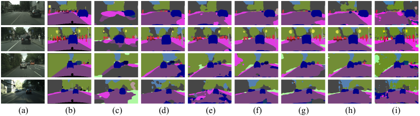
Figure 3: Qualitative semantic segmentation result from GTA and SYNTHIA to Cityscapes. From left to right are: (a) original image, (b) ground truth annotation, (c) source only from GTA, (d) CycleGANs on GTA and SYNTHIA, (e) +CCD+DSC, (f) +SAD+DSC, (g) +CCD+SAD+DSC, (h) +CCD+SAD+DSC+FLA (MADAN), and (i) +CCD+SAD+DSC+FLA+CLA+CAG (MADAN+).

Table X: Comparison between the proposed dynamic semantic consistency (DSC) loss in MADAN and the original SC loss in [27] on Cityscapes using FCN-VGG16 backbone. The better mIoU for each pair is emphasized in bold.

Source	Method	road	sidewalk	building	wall	fence	pole	t-light	t-sign	vegettion	sky	person	rider	car	bus	m-bike	bicycle	mIoU
	CycleGAN+SC	85.6	30.7	74.7	14.4	13.0	17.6	13.7	5.8	74.6	69.9	38.2	3.5	72.3	5.0	3.6	0.0	32.7
	CycleGAN+DSC	76.6	26.0	76.3	17.3	18.8	13.6	13.2	17.9	78.8	63.9	47.4	14.8	72.2	24.1	19.8	10.8	38.1
	CyCADA w/ SC	85.2	37.2	76.5	21.8	15.0	23.8	21.5	22.9	80.5	60.7	50.5	9.0	76.9	28.2	9.8	0.0	38.7
GTA	CyCADA w/ DSC	84.1	27.3	78.3	21.6	18.0	13.8	14.1	16.7	78.1	66.9	47.8	15.4	78.7	23.4	22.3	14.4	40.0
	CycleGAN+SC	64.0	29.4	61.7	0.3	0.1	15.3	3.4	5.0	63.4	68.4	39.4	11.5	46.6	10.4	2.0	16.4	27.3
	CycleGAN + DSC	68.4	29.0	65.2	0.6	0.0	15.0	0.1	4.0	75.1	70.6	45.0	11.0	54.9	18.2	3.9	26.7	30.5
	CyCADA w/ SC	66.2	29.6	65.3	0.5	0.2	15.1	4.5	6.9	67.1	68.2	42.8	14.1	51.2	12.6	2.4	20.7	29.2
SYNTHIA	CyCADA w/ DSC	69.8	27.2	68.5	5.8	0.0	11.6	0.0	2.8	75.7	58.3	44.3	10.5	68.1	22.1	11.8	32.7	31.8

Table XI: Comparison between the proposed dynamic semantic consistency (DSC) loss in MADAN and the original SC loss in [27] on BDDS using FCN-VGG16 backbone. The better mIoU for each pair is emphasized in bold.

Source	Method	road	sidewalk	building	wall	fence	pole	t-light	t-sign	vegettion	sky	person	rider	car	bus	m-bike	bicycle	mIoU
	CycleGAN+SC	62.1	20.9	59.2	6.0	23.5	12.8	9.2	22.4	65.9	78.4	34.7	11.4	64.4	14.2	10.9	1.9	31.1
	CycleGAN+DSC	74.4	23.7	65.0	8.6	17.2	10.7	14.2	19.7	59.0	82.8	36.3	19.6	69.7	4.3	17.6	4.2	32.9
	CyCADA w/ SC	68.8	23.7	67.0	7.5	16.2	9.4	11.3	22.2	60.5	82.1	36.1	20.6	63.2	15.2	16.6	3.4	32.0
GTA	CyCADA w/ DSC	70.5	32.4	68.2	10.5	17.3	18.4	16.6	21.8	65.6	82.2	38.1	16.1	73.3	20.8	12.6	3.7	35.5
	CycleGAN+SC	50.6	13.6	50.5	0.2	0.0	7.9	0.0	0.0	63.8	58.3	21.6	7.8	50.2	1.8	2.2	19.9	21.8
	CycleGAN + DSC	57.3	13.4	56.1	2.7	14.1	9.8	7.7	17.1	65.5	53.1	11.4	1.4	51.4	13.9	3.9	8.7	22.5
	CyCADA w/ SC	49.5	11.1	46.6	0.7	0.0	10.0	0.4	7.0	61.0	74.6	17.5	7.2	50.9	5.8	13.1	4.3	23.4
SYNTHIA	CyCADA w/ DSC	55.0	13.8	45.2	0.1	0.0	13.2	0.5	10.6	63.3	67.4	22.0	6.9	52.5	10.5	10.4	13.3	24.0

(1) The source-only method that directly transfers the task models trained on the source domains to the target domain obtains the worst performance in most adaptation settings. This is obvious, because the joint probability distributions of observed images and labels are significantly different among the sources and the target, due to the presence of domain shift. Without domain adaptation, the direct transfer cannot well handle this domain gap.

(2) Comparing source-only with corresponding single-best DA and source-combined DA for digit recognition and object classification, and comparing source-only with single-source DA for semantic segmentation, it is clear that almost all adaptation methods perform better than source-only, which demonstrates the effectiveness of domain adaptation. For example, in Table III, the average accuracy of source-only combined method is 80.2%, while the accuracy of source-combined ADDA is 83.7%.

Table XII: Ablation study on different components in MADAN+ on Cityscapes using FCN-VGG16 backbone. Baseline denotes using pixel-level alignment with cycle-consistency, +SAD denotes using the sub-domain aggregation discriminator, +CCD denotes using the cross-domain cycle discriminator, +DSC denotes using the dynamic semantic consistency loss, +FLA denotes using feature-level alignment, +CAG denotes using context-aware generation.

Method	road	sidewalk	building	wall	fence	pole	t-light	t-sign	vegettion	sky	person	rider	car	bus	m-bike	bicycle	mIoU
Baseline	74.9	27.6	67.5	9.1	10.0	12.8	1.4	13.6	63.0	47.1	41.7	13.5	60.8	22.4	6.0	8.1	30.0
+SAD	79.7	33.2	75.9	11.8	3.6	15.9	8.6	15.0	74.7	78.9	44.2	17.1	68.2	24.9	16.7	14.0	36.4
+CCD	82.1	36.3	69.8	9.5	4.9	11.8	12.5	15.3	61.3	54.1	49.7	10.0	70.7	9.7	19.7	12.4	33.1
+SAD+CCD	82.7	35.3	76.5	15.4	19.4	14.1	7.2	13.9	75.3	74.2	50.9	19.0	66.5	26.6	16.3	6.7	37.5
+SAD+DSC	83.1	36.6	78.0	23.3	12.6	11.8	3.5	11.3	75.5	74.8	42.2	17.9	72.2	27.2	13.8	10.0	37.1
+CCD+DSC	86.8	36.9	78.6	16.2	8.1	17.7	8.9	13.7	75.0	74.8	42.2	18.2	74.6	22.5	22.9	12.7	38.1
+SAD+CCD+DSC	84.2	35.1	78.7	17.1	18.7	15.4	15.7	24.1	77.9	72.0	49.2	17.1	75.2	24.1	18.9	19.2	40.2
SAD+CCD+DSC+FLA	86.2	37.7	79.1	20.1	17.8	15.5	14.5	21.4	78.5	73.4	49.7	16.8	77.8	28.3	17.7	27.5	41.4
+SAD+CCD+DSC+FLA+CLA	87.7	45.2	80.2	24.0	12.4	16.0	13.4	14.8	79.8	76.7	49.7	20.8	79.9	24.9	19.5	20.6	41.6
+SAD+CCD+DSC+FLA+CLA+CAG	87.9	41.0	76.4	21.4	1.3	28.4	20.3	22.3	77.3	80.0	54.9	21.5	80.1	29.7	15.1	26.5	42.8

Table XIII: Ablation study on different components in MADAN+ on BDDS using FCN-VGG16 backbone.

Method	road	sidewalk	building	wall	fence	pole	t-light	t-sign	vegettion	sky	person	rider	car	bus	m-bike	bicycle	mIoU
Baseline	31.3	17.4	55.4	2.6	12.9	12.4	6.5	18.0	63.2	79.9	21.2	5.6	44.1	14.2	6.1	11.7	24.6
+SAD	58.9	18.7	61.8	6.4	10.7	17.1	20.3	17.0	67.3	83.7	21.1	6.7	66.6	22.7	4.5	14.9	31.2
+CCD	52.7	13.6	63.0	6.6	11.2	17.8	21.5	18.9	67.4	84.0	9.2	2.2	63.0	21.6	2.0	14.0	29.3
+SAD+CCD	61.6	20.2	61.7	7.2	12.1	18.5	19.8	16.7	64.2	83.2	25.9	7.3	66.8	22.2	5.3	14.9	31.8
+SAD+DSC	60.2	29.5	66.6	16.9	10.0	16.6	10.9	16.4	78.8	75.1	47.5	17.3	48.0	24.0	13.2	17.3	34.3
+CCD+DSC	61.5	27.6	72.1	6.5	12.8	15.7	10.8	18.1	78.3	73.8	44.9	16.3	41.5	21.1	21.8	15.9	33.7
+SAD+CCD+DSC	64.6	38.0	75.8	17.8	13.0	9.8	5.9	4.6	74.8	76.9	41.8	24.0	69.0	20.4	23.7	11.3	35.3
+SAD+CCD+DSC+FLA	69.1	36.3	77.9	21.5	17.4	13.8	4.1	16.2	76.5	76.2	42.2	16.4	56.3	22.4	24.5	13.5	36.3
+SAD+CCD+DSC+FLA+CLA	75.1	30.5	70.8	10.3	11.5	27.8	10.6	15.9	80.6	80.9	51.0	12.2	67.2	21.3	17.2	22.4	37.8
+SAD+CCD+DSC+FLA+CLA+CAG	75.2	29.8	83.3	27.2	20.7	37.8	23.2	20.6	81.1	83.5	50.1	9.8	80.2	13.2	11.6	18.1	41.6

(3) Generally, multi-source DA outperforms other adaptation standards by exploring the complementarity of different sources. This is more obvious when comparing the DA methods that employ similar architectures, such as our MADAN vs. CyCADA [27], MDDA [30] vs. ADDA [17], and MDAN [42] vs. DANN [61]. Besides the domain gap between the sources and the target, multi-source DA also tries to bridge the domain gap across different sources. This demonstrates the necessity and superiority of multi-source DA over single-source DA.

(4) MADAN achieves the best average results among all adaptation methods, benefiting from the joint consideration of pixel-level and feature-level alignments, cycle-consistency, dynamic semantic consistency, domain aggregation, and multiple sources. MADAN also significantly outperforms source-combined DA, in which domain shift also exists among different sources. By bridging this gap, multi-source DA can boost the adaptation performance. On the one hand, compared to single-source DA like CyCADA [27], MADAN utilizes more useful information from multiple sources. On the other hand, other multi-source DA methods [41, 42, 43, 30] only consider feature-level alignment, which is obviously insufficient especially for fine-grained tasks, e.g. semantic segmentation, a pixel-wise prediction task. In addition, we consider pixel-level alignment with a dynamic semantic consistency loss and further aggregate different adapted domains.

(5) Take segmentation segmentation for example, the oracle method that is trained on the target domain performs significantly better than the others. However, to train this model, the ground truth labels from the target domain are required, which are actually unavailable in UDA settings. We can deem this performance as a upper bound of UDA. Obviously, there is still a large performance gap between all adaptation algorithms and the oracle method, requiring further efforts on DA.

There are also some task-specific observations:

(1) Simply combining different source domains into one source and performing source-only or single-source DA does not guarantee better performance than corresponding single-best method. For example, for the source-only standard, the single-best method outperforms the combined method on Digits-five, Office-31, Office+Caltech-10 datasets, while the combined method performs better on Office-Home, Cityscapes, and BDDS datasets. For the single-source DA, we usually have opposite observations. For example, in Table VI, the mIoUs of CyCADA from GTA to Cityscapes and from SYNTHIA to Cityscapes are 38.7% and 29.2%, while the mIoU of source-combined DA is 37.3%. Currently, there is no accurate explanation on this observation. On the one hand, combining multiple sources into one source results in more training data, which can intuitively boost the performance. On the other hand, the data from different sources are collected from different distributions, which may interfere with each other. Therefore, the comparison between the single-best method and the combined method depends on which aspect is stronger.

(2) For semantic segmentation adaptation, MADAN+ outperforms MADAN with a remarkable margin. For example, the average performance gains of MADAN+ over MADAN using DeepLabV2 backbone are 3.1% and 2.3% on Cityscapges and BDDS, respectively. Further, MADAN+ achieves the best cwIoU scores of 6 to 9 out of 16 categories. These results demonstrate the superiority of MDAN+ over MADAN for pixel-wise segmentation adaptation with the help of category-level alignment and context-aware generation.

Segmentation Visualization. The qualitative semantic segmentation results are shown in Figure 3. We can clearly see that after adaptation by the proposed method, the visual segmentation results are improved notably, which look more similar to the ground truth (b). Take the second row for example, the contours of pedestrians and cyclists by MADAN+ (i) are more clear than those by the methods of source only (c) and CycleGAN (d).

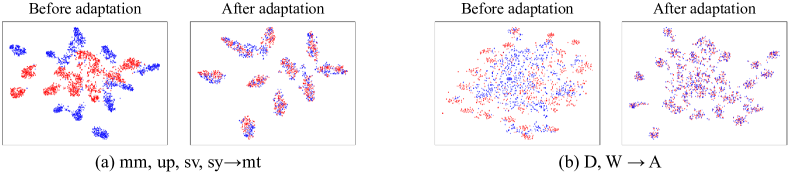
Figure 4: The t-SNE [91] visualization of the learned features for task (a) Digits-five: mm, up, sv, sy$\rightarrow$mt and (b) Office-31: D, W$\rightarrow$A. In each pair, the features are extracted using the last layer of source domain encoder from the samples of source and target domain in the first image, and the target domain features are extracted using the the last layer of adapted encoder in the second one.

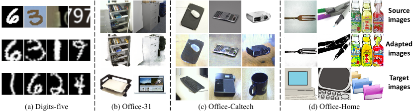
Figure 5: Visualization of image translation for classification adaptation. From left to right are: (a) Digits-five: mt, mm, sv, sy $\rightarrow$ up, (b) Office-31: W, D $\rightarrow$ A, (c), Office+Caltech-10: D, C, A $\rightarrow$ W (d) Office-Home: Ar, Rw, Pr $\rightarrow$ Cl. Red: source, blue: target.

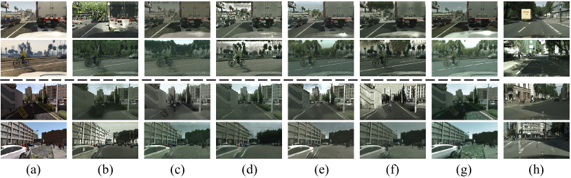
Figure 6: Visualization of image translation for segmentation adaptation from GTA and SYNTHIA to Cityscapes. From left to right are: (a) original source image, (b) CycleGAN, (c) CycleGAN+DSC, (d) CycleGAN+CCD+DSC, (e) CycleGAN+SAD+DSC, (f) CycleGAN+CCD+SAD+DSC, (g) CycleGAN+CCD+SAD+CAG, and (h) target Cityscapes image. The top two rows and bottom rows are GTA $\rightarrow$ Cityscapes and SYNTHIA $\rightarrow$ Cityscapes, respectively.

5.3 Ablation Study

To demonstrate the effectiveness of different components in the proposed MADAN and MADAN+ models, we conduct ablation studies on the segmentation adaptation tasks.

First, we compare the proposed dynamic semantic consistency (DSC) loss with the original semantic consistency (SC) loss [27] using the DA methods of CycleGAN [47] and CyCADA [27]. The results on Cityscapes and BDDS are shown in Table X and Table XI, respectively. We can see that for all adaptation settings, DSC achieves better mIoU results than SC. For example, the mIoU improvements of DSC over SC in CycleGAN and CyCADA from GTA to Cityscapes are 5.4% and 1.3%, respectively, while the corresponding improvements are 3.2% and 2.6% from SYNTHIA to Cityscapes. These results demonstrate the effectiveness of our proposed DSC loss.

Second, we incrementally evaluate the influence of different components in MADAN+. The results on Cityscapes and BDDS using FCN-VGG16 backbone are shown in Table XII and Table XIII, respectively. We have several observations. (1) Both domain aggregation methods, i.e. SAD and CCD, obtain larger mIoU scores than baseline with SAD performing better. The performance gains are obtained by making different adapted domains more closely aggregated. (2) Adding the DSC loss could further improve the segmentation performance, again demonstrating the effectiveness of DSC. (3) feature-level alignment is also helpful with 1.2% and 1.0% improvements on Cityscapes and BDDS, respectively, obviously contributing to the adaptation task. (4) Category-level alignment (CLA) is complementary to the feature-level alignment (FLA). While FLA aims to align the target and source features globally, CLA makes the features in local regions indistinguishable. (5) context-aware generation (CAG) significantly contributes to the adaptation task. (6) The modules are orthogonal to each other to some extent, since adding each one of them does not introduce performance degradation. (7) As compared to MADAN, MADAN+ achieves better results with 1.4% and 5.3% performance gains on Cityscapes and BDDS, respectively. Moreover, by adding CLA and CAG, the cwIoU of most categories are increased. These results demonstrate the superiority of MADAN+ over MADAN for pixel-wise adaptation.

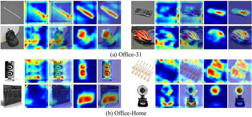
Figure 7: Comparison of the attention maps before and after adaptation on (a) Office-31 and (b) Office-Home datasets. For each group, the five columns from left to right are: the original target image, attention map before adaptation, image with attention map before adaptation, attention map after adaptation, and image with attention map after adaptation. Red regions indicate more attention.

5.4 Feature Visualization

To show the feature transferability of the proposed MADAN model, we visualize the features before and after adaptation with t-SNE embedding [91] in two tasks: (a) Digits-five: mm, up, sv, sy$\rightarrow$mt and (b) Office-31: D, W$\rightarrow$A. As illustrated in Figure 4, we can observe that after adaptation, the target domain is more indistinguishable from the source domains, which demonstrates that the proposed MADAN model can align the distributions between the source and target domains. Based on the more transferable features after adaptation, the task classifier learned on the source domains can work well on the target domain, leading high task performance on the target domain.

5.5 Model Interpretability

We visualize the results of pixel-level alignment (PLA) and attention maps before and after adaptation to demonstrate the interpretability of our model. First, we show the comparison among source image, adapted images, and target images for classification and segmentation adaptation in Figure 5 and Figure 6, respectively. We can see that the styles of the adapted images by our PLA method are closer to the target than the source to the target. Meanwhile, the semantic information is well preserved. For classification in Figure 5: (a) although styles of the source images are different, the corresponding adapted images are uniformly changed to the handwritten brush style of the target images; (b) the background is removed in the adapted images; (c) a desktop background is added to the adapted images; (d) the adapted images are cartooned to have similar styles to the target images. For segmentation in Figure 6, comparing the columns from (a) to (g) with the column (h) especially (a) vs. (h) and (g) vs. (h), we can observe that with our final FLA method (g), the styles (e.g. overall hue and brightness) of the adapted images are much more similar to the target Cityscapes.

Second, we visualize the attention before and after the proposed domain adaptation method using the heat map generated by the Grad-Cam algorithm [92]. The comparison before and after adaptation on Office-31 and Office-Home datasets are illustrated in Figure 7. It is clear that different regions in the images have different attentions but the attentions generated by our domain adaptation method can focus more on the desirable and discriminative regions. For example, on the Office-31 dataset, for the image in the top right group, the calculator is highlighted with more attention after adaptation, while more attention is focused on a region in the background before adaptation; for the image in the bottom right group, after adaptation more attention is paid to the helmet and the attention diminishes for the complex background with messy objects. On the Office-Home dataset, for the image in the top left group, the attention before adaptation focuses on the background and the edge of the speaker, while the more discriminative and transferable trumpets are emphasized after adaptation; for the image in the bottom right group, only the lens of the Webcam is highlighted after adaptation since it is more transferable than the base of the camera. These observations intuitively demonstrate that the attended regions by our adaptation model are invariant across different domains and discriminative for the learning task.

6 Conclusion

In this paper, we proposed a novel framework, termed Multi-source Adversarial Domain Aggregation Network (MADAN), for multi-source domain adaptation (MDA). For each source domain, based on cycle-consistent GAN at pixel-level alignment, we first generated adapted images with a novel dynamic semantic consistency loss. Further, we proposed a sub-domain aggregation discriminator and cross-domain cycle discriminator to better aggregate different adapted domains. Finally, we trained the task model using the adapted images in the aggregated domain and corresponding labels in the source domains. The experiments showed that MADAN achieves 2.8%, 3.0%, 2.2%, and 4.6% classification accuracy improvements compared with the existing best MDA methods, respectively on Digits-five, Office-31, Office+Caltech-10, and Office-Home datasets. We also studied MDA for semantic segmentation, which is the first work on adapting pixel-wise prediction task with multiple sources. To better deal with the pixel-wise adaptation, we extended MDAN to MADAN+ with category-level alignment and context-aware generation. For the FCN-VGG16 backbone, MADAN+ achieves 17.0%, 3.0%, 5.5%, and 13.4% mIoU improvements compared with best source-only, best single-source DA, source-combined DA, and other multi-source DA, respectively on Cityscapes from GTA and SYNTHIA, and 17.0%, 5.9%, 7.9%, 16.6% on BDDS.

For future studies, we plan to investigate multi-modal DA, such as using both image and LiDAR data, to further boost the adaptation performance. Improving the computational efficiency of MADAN, with techniques such as neural architecture search, is another direction worth investigating. In addition, we will study how to automatically weigh the relative importance of different sources and the samples in each source to further improve the performance of MADAN.

Acknowledgments

This work is supported by Berkeley DeepDrive and the National Natural Science Foundation of China (No. 61701273).

References

- Krizhevsky et al. [2012] A. Krizhevsky, I. Sutskever, and G. E. Hinton, “Imagenet classification with deep convolutional neural networks,” in Advances in Neural Information Processing Systems, 2012, pp. 1097–1105.
- Simonyan and Zisserman [2014] K. Simonyan and A. Zisserman, “Very deep convolutional networks for large-scale image recognition,” in International Conference on Learning Representations, 2014.
- He et al. [2016] K. He, X. Zhang, S. Ren, and J. Sun, “Deep residual learning for image recognition,” in IEEE conference on Computer Vision and Pattern Recognition, 2016, pp. 770–778.
- Huang et al. [2017] G. Huang, Z. Liu, L. Van Der Maaten, and K. Q. Weinberger, “Densely connected convolutional networks,” in IEEE conference on Computer Vision and Pattern Recognition, 2017, pp. 4700–4708.
- Girshick [2015] R. Girshick, “Fast r-cnn,” in IEEE International Conference on Computer Vision, 2015, pp. 1440–1448.
- Ren et al. [2015] S. Ren, K. He, R. Girshick, and J. Sun, “Faster r-cnn: Towards real-time object detection with region proposal networks,” in Advances in Neural Information Processing Systems, 2015, pp. 91–99.
- Redmon et al. [2016] J. Redmon, S. Divvala, R. Girshick, and A. Farhadi, “You only look once: Unified, real-time object detection,” in IEEE conference on Computer Vision and Pattern Recognition, 2016, pp. 779–788.
- Long et al. [2015a] J. Long, E. Shelhamer, and T. Darrell, “Fully convolutional networks for semantic segmentation,” in IEEE Conference on Computer Vision and Pattern Recognition, 2015, pp. 3431–3440.
- Badrinarayanan et al. [2017] V. Badrinarayanan, A. Kendall, and R. Cipolla, “Segnet: A deep convolutional encoder-decoder architecture for image segmentation,” IEEE Transactions on Pattern Analysis and Machine Intelligence, vol. 39, no. 12, pp. 2481–2495, 2017.
- Chen et al. [2017a] L.-C. Chen, G. Papandreou, I. Kokkinos, K. Murphy, and A. L. Yuille, “Deeplab: Semantic image segmentation with deep convolutional nets, atrous convolution, and fully connected crfs,” IEEE Transactions on Pattern Analysis and Machine Intelligence, vol. 40, no. 4, pp. 834–848, 2017.
- Gebru et al. [2017] T. Gebru, J. Hoffman, and L. Fei-Fei, “Fine-grained recognition in the wild: A multi-task domain adaptation approach,” in IEEE International Conference on Computer Vision, 2017, pp. 1358–1367.
- Cordts et al. [2016] M. Cordts, M. Omran, S. Ramos, T. Rehfeld, M. Enzweiler, R. Benenson, U. Franke, S. Roth, and B. Schiele, “The cityscapes dataset for semantic urban scene understanding,” in IEEE Conference on Computer Vision and Pattern Recognition, 2016, pp. 3213–3223.
- Wu et al. [2019] B. Wu, X. Zhou, S. Zhao, X. Yue, and K. Keutzer, “Squeezesegv2: Improved model structure and unsupervised domain adaptation for road-object segmentation from a lidar point cloud,” in IEEE International Conference on Robotics and Automation, 2019, pp. 4376–4382.
- Yue et al. [2018] X. Yue, B. Wu, S. A. Seshia, K. Keutzer, and A. L. Sangiovanni-Vincentelli, “A lidar point cloud generator: from a virtual world to autonomous driving,” in ACM International Conference on Multimedia Retrieval, 2018, pp. 458–464.
- Torralba and Efros [2011] A. Torralba and A. A. Efros, “Unbiased look at dataset bias,” in IEEE Conference on Computer Vision and Pattern Recognition, 2011, pp. 1521–1528.
- Bousmalis et al. [2016] K. Bousmalis, G. Trigeorgis, N. Silberman, D. Krishnan, and D. Erhan, “Domain separation networks,” in Advances in Neural Information Processing Systems, 2016, pp. 343–351.
- Tzeng et al. [2017] E. Tzeng, J. Hoffman, K. Saenko, and T. Darrell, “Adversarial discriminative domain adaptation,” in IEEE Conference on Computer Vision and Pattern Recognition, 2017, pp. 2962–2971.
- Ben-David et al. [2010] S. Ben-David, J. Blitzer, K. Crammer, A. Kulesza, F. Pereira, and J. W. Vaughan, “A theory of learning from different domains,” Machine learning, vol. 79, no. 1-2, pp. 151–175, 2010.
- Gopalan et al. [2014] R. Gopalan, R. Li, and R. Chellappa, “Unsupervised adaptation across domain shifts by generating intermediate data representations,” IEEE Transactions on Pattern Analysis and Machine Intelligence, vol. 36, no. 11, pp. 2288–2302, 2014.
- Louizos et al. [2015] C. Louizos, K. Swersky, Y. Li, M. Welling, and R. Zemel, “The variational fair autoencoder,” arXiv:1511.00830, 2015.
- Pan and Yang [2010] S. J. Pan and Q. Yang, “A survey on transfer learning,” IEEE Transactions on Knowledge and Data Engineering, vol. 22, no. 10, pp. 1345–1359, 2010.
- Glorot et al. [2011] X. Glorot, A. Bordes, and Y. Bengio, “Domain adaptation for large-scale sentiment classification: A deep learning approach,” in International Conference on Machine Learning, 2011, pp. 513–520.
- Jhuo et al. [2012] I.-H. Jhuo, D. Liu, D. Lee, and S.-F. Chang, “Robust visual domain adaptation with low-rank reconstruction,” in IEEE Conference on Computer Vision and Pattern Recognition, 2012, pp. 2168–2175.
- Becker et al. [2013] C. J. Becker, C. M. Christoudias, and P. Fua, “Non-linear domain adaptation with boosting,” in Advances in Neural Information Processing Systems, 2013, pp. 485–493.
- Ghifary et al. [2015] M. Ghifary, W. Bastiaan Kleijn, M. Zhang, and D. Balduzzi, “Domain generalization for object recognition with multi-task autoencoders,” in IEEE International Conference on Computer Vision, 2015, pp. 2551–2559.
- Long et al. [2015b] M. Long, Y. Cao, J. Wang, and M. Jordan, “Learning transferable features with deep adaptation networks,” in International Conference on Machine Learning, 2015, pp. 97–105.
- Hoffman et al. [2018a] J. Hoffman, E. Tzeng, T. Park, J.-Y. Zhu, P. Isola, K. Saenko, A. A. Efros, and T. Darrell, “Cycada: Cycle-consistent adversarial domain adaptation,” in International Conference on Machine Learning, 2018, pp. 1994–2003.
- Zhao et al. [2019a] S. Zhao, C. Lin, P. Xu, S. Zhao, Y. Guo, R. Krishna, G. Ding, and K. Keutzer, “Cycleemotiongan: Emotional semantic consistency preserved cyclegan for adapting image emotions,” in AAAI Conference on Artificial Intelligence, 2019, pp. 2620–2627.
- Sun et al. [2015] S. Sun, H. Shi, and Y. Wu, “A survey of multi-source domain adaptation,” Information Fusion, vol. 24, pp. 84–92, 2015.
- Zhao et al. [2020] S. Zhao, G. Wang, S. Zhang, Y. Gu, Y. Li, Z. Song, P. Xu, R. Hu, H. Chai, and K. Keutzer, “Multi-source distilling domain adaptation,” in AAAI Conference on Artificial Intelligence, 2020.
- Riemer et al. [2019] M. Riemer, I. Cases, R. Ajemian, M. Liu, I. Rish, Y. Tu, and G. Tesauro, “Learning to learn without forgetting by maximizing transfer and minimizing interference,” in International Conference on Learning Representations, 2019.
- Duan et al. [2009] L. Duan, I. W. Tsang, D. Xu, and T.-S. Chua, “Domain adaptation from multiple sources via auxiliary classifiers,” in International Conference on Machine Learning, 2009, pp. 289–296.
- Sun et al. [2011] Q. Sun, R. Chattopadhyay, S. Panchanathan, and J. Ye, “A two-stage weighting framework for multi-source domain adaptation,” in Advances in Neural Information Processing Systems, 2011, pp. 505–513.
- Duan et al. [2012a] L. Duan, D. Xu, and S.-F. Chang, “Exploiting web images for event recognition in consumer videos: A multiple source domain adaptation approach,” in IEEE Conference on Computer Vision and Pattern Recognition, 2012, pp. 1338–1345.
- Chattopadhyay et al. [2012] R. Chattopadhyay, Q. Sun, W. Fan, I. Davidson, S. Panchanathan, and J. Ye, “Multisource domain adaptation and its application to early detection of fatigue,” ACM Transactions on Knowledge Discovery from Data, vol. 6, no. 4, p. 18, 2012.
- Duan et al. [2012b] L. Duan, D. Xu, and I. W.-H. Tsang, “Domain adaptation from multiple sources: A domain-dependent regularization approach,” IEEE Transactions on Neural Networks and Learning Systems, vol. 23, no. 3, pp. 504–518, 2012.
- Yang et al. [2007] J. Yang, R. Yan, and A. G. Hauptmann, “Cross-domain video concept detection using adaptive svms,” in ACM International Conference on Multimedia, 2007, pp. 188–197.
- Schweikert et al. [2009] G. Schweikert, G. Rätsch, C. Widmer, and B. Schölkopf, “An empirical analysis of domain adaptation algorithms for genomic sequence analysis,” in Advances in Neural Information Processing Systems, 2009, pp. 1433–1440.
- Xu and Sun [2012] Z. Xu and S. Sun, “Multi-source transfer learning with multi-view adaboost,” in International Conference on Neural Information Processing, 2012, pp. 332–339.
- Sun and Shi [2013] S.-L. Sun and H.-L. Shi, “Bayesian multi-source domain adaptation,” in International Conference on Machine Learning and Cybernetics, vol. 1, 2013, pp. 24–28.
- Xu et al. [2018] R. Xu, Z. Chen, W. Zuo, J. Yan, and L. Lin, “Deep cocktail network: Multi-source unsupervised domain adaptation with category shift,” in IEEE Conference on Computer Vision and Pattern Recognition, 2018, pp. 3964–3973.
- Zhao et al. [2018] H. Zhao, S. Zhang, G. Wu, J. M. Moura, J. P. Costeira, and G. J. Gordon, “Adversarial multiple source domain adaptation,” in Advances in Neural Information Processing Systems, 2018, pp. 8568–8579.
- Peng et al. [2019] X. Peng, Q. Bai, X. Xia, Z. Huang, K. Saenko, and B. Wang, “Moment matching for multi-source domain adaptation,” in IEEE International Conference on Computer Vision, 2019, pp. 1406–1415.
- Zhang et al. [2017] Y. Zhang, P. David, and B. Gong, “Curriculum domain adaptation for semantic segmentation of urban scenes,” in IEEE International Conference on Computer Vision, 2017, pp. 2020–2030.
- Tsai et al. [2018] Y.-H. Tsai, W.-C. Hung, S. Schulter, K. Sohn, M.-H. Yang, and M. Chandraker, “Learning to adapt structured output space for semantic segmentation,” in IEEE Conference on Computer Vision and Pattern Recognition, 2018, pp. 7472–7481.
- Goodfellow et al. [2014] I. Goodfellow, J. Pouget-Abadie, M. Mirza, B. Xu, D. Warde-Farley, S. Ozair, A. Courville, and Y. Bengio, “Generative adversarial nets,” in Advances in Neural Information Processing Systems, 2014, pp. 2672–2680.
- Zhu et al. [2017] J.-Y. Zhu, T. Park, P. Isola, and A. A. Efros, “Unpaired image-to-image translation using cycle-consistent adversarial networks,” in IEEE International Conference on Computer Vision, 2017, pp. 2223–2232.
- Zhao et al. [2019b] S. Zhao, B. Li, X. Yue, Y. Gu, P. Xu, R. Hu, H. Chai, and K. Keutzer, “Multi-source domain adaptation for semantic segmentation,” in Advances in Neural Information Processing Systems, 2019, pp. 7285–7298.
- Bousmalis et al. [2017] K. Bousmalis, N. Silberman, D. Dohan, D. Erhan, and D. Krishnan, “Unsupervised pixel-level domain adaptation with generative adversarial networks,” in IEEE Conference on Computer Vision and Pattern Recognition, 2017, pp. 3722–3731.
- Chen et al. [2017b] Y.-H. Chen, W.-Y. Chen, Y.-T. Chen, B.-C. Tsai, Y.-C. Frank Wang, and M. Sun, “No more discrimination: Cross city adaptation of road scene segmenters,” in IEEE International Conference on Computer Vision, 2017, pp. 1992–2001.
- Russo et al. [2018] P. Russo, F. M. Carlucci, T. Tommasi, and B. Caputo, “From source to target and back: symmetric bi-directional adaptive gan,” in IEEE Conference on Computer Vision and Pattern Recognition, 2018, pp. 8099–8108.
- Sankaranarayanan et al. [2018] S. Sankaranarayanan, Y. Balaji, C. D. Castillo, and R. Chellappa, “Generate to adapt: Aligning domains using generative adversarial networks,” in IEEE Conference on Computer Vision and Pattern Recognition, 2018, pp. 8503–8512.
- Hu et al. [2018] L. Hu, M. Kan, S. Shan, and X. Chen, “Duplex generative adversarial network for unsupervised domain adaptation,” in IEEE Conference on Computer Vision and Pattern Recognition, 2018, pp. 1498–1507.
- Patel et al. [2015] V. M. Patel, R. Gopalan, R. Li, and R. Chellappa, “Visual domain adaptation: A survey of recent advances,” IEEE Signal Processing Magazine, vol. 32, no. 3, pp. 53–69, 2015.
- Zhuo et al. [2017] J. Zhuo, S. Wang, W. Zhang, and Q. Huang, “Deep unsupervised convolutional domain adaptation,” in ACM International Conference on Multimedia, 2017, pp. 261–269.
- Sun et al. [2016] B. Sun, J. Feng, and K. Saenko, “Return of frustratingly easy domain adaptation,” in AAAI Conference on Artificial Intelligence, 2016, pp. 2058–2065.
- Kang et al. [2019] G. Kang, L. Jiang, Y. Yang, and A. G. Hauptmann, “Contrastive adaptation network for unsupervised domain adaptation,” in IEEE Conference on Computer Vision and Pattern Recognition, 2019, pp. 4893–4902.
- Liu and Tuzel [2016] M.-Y. Liu and O. Tuzel, “Coupled generative adversarial networks,” in Advances in Neural Information Processing Systems, 2016, pp. 469–477.
- Shrivastava et al. [2017] A. Shrivastava, T. Pfister, O. Tuzel, J. Susskind, W. Wang, and R. Webb, “Learning from simulated and unsupervised images through adversarial training,” in IEEE Conference on Computer Vision and Pattern Recognition, 2017, pp. 2242–2251.
- Yue et al. [2019] X. Yue, Y. Zhang, S. Zhao, A. Sangiovanni-Vincentelli, K. Keutzer, and B. Gong, “Domain randomization and pyramid consistency: Simulation-to-real generalization without accessing target domain data,” in IEEE International Conference on Computer Vision, 2019, pp. 2100–2110.
- Ganin et al. [2016] Y. Ganin, E. Ustinova, H. Ajakan, P. Germain, H. Larochelle, F. Laviolette, M. Marchand, and V. Lempitsky, “Domain-adversarial training of neural networks,” Journal of Machine Learning Research, vol. 17, no. 1, pp. 2096–2030, 2016.
- Shen et al. [2017] J. Shen, Y. Qu, W. Zhang, and Y. Yu, “Wasserstein distance guided representation learning for domain adaptation,” arXiv:1707.01217, 2017.
- Huang et al. [2018] H. Huang, Q. Huang, and P. Krahenbuhl, “Domain transfer through deep activation matching,” in European Conference on Computer Vision, 2018, pp. 590–605.
- Ghifary et al. [2016] M. Ghifary, W. B. Kleijn, M. Zhang, D. Balduzzi, and W. Li, “Deep reconstruction-classification networks for unsupervised domain adaptation,” in European Conference on Computer Vision, 2016, pp. 597–613.
- Hoffman et al. [2018b] J. Hoffman, M. Mohri, and N. Zhang, “Algorithms and theory for multiple-source adaptation,” in Advances in Neural Information Processing Systems, 2018, pp. 8246–8256.
- Ding et al. [2018] Z. Ding, M. Shao, and Y. Fu, “Incomplete multisource transfer learning,” IEEE Transactions on Neural Networks and Learning Systems, vol. 29, no. 2, pp. 310–323, 2018.
- Redko et al. [2019] I. Redko, N. Courty, R. Flamary, and D. Tuia, “Optimal transport for multi-source domain adaptation under target shift,” in International Conference on Artificial Intelligence and Statistics, 2019, pp. 849–858.
- LeCun et al. [1998] Y. LeCun, L. Bottou, Y. Bengio, P. Haffner et al., “Gradient-based learning applied to document recognition,” Proceedings of the IEEE, vol. 86, no. 11, pp. 2278–2324, 1998.
- Ganin and Lempitsky [2015] Y. Ganin and V. Lempitsky, “Unsupervised domain adaptation by backpropagation,” in International Conference on Machine Learning, 2015, pp. 1180–1189.
- Netzer et al. [2011] Y. Netzer, T. Wang, A. Coates, A. Bissacco, B. Wu, and A. Y. Ng, “Reading digits in natural images with unsupervised feature learning,” in Advances in Neural Information Processing Systems Workshops, 2011.
- Hull [1994] J. J. Hull, “A database for handwritten text recognition research,” IEEE Transactions on Pattern Analysis and Machine Intelligence, vol. 16, no. 5, pp. 550–554, 1994.
- Saenko et al. [2010] K. Saenko, B. Kulis, M. Fritz, and T. Darrell, “Adapting visual category models to new domains,” in European Conference on Computer Vision, 2010, pp. 213–226.
- Gong et al. [2013] B. Gong, K. Grauman, and F. Sha, “Connecting the dots with landmarks: Discriminatively learning domain-invariant features for unsupervised domain adaptation,” in International Conference on Machine Learning, 2013, pp. 222–230.
- Griffin et al. [2007] G. Griffin, A. Holub, and P. Perona, “Caltech-256 object category dataset,” 2007.
- Venkateswara et al. [2017] H. Venkateswara, J. Eusebio, S. Chakraborty, and S. Panchanathan, “Deep hashing network for unsupervised domain adaptation,” in IEEE Conference on Computer Vision and Pattern Recognition, 2017, pp. 5018–5027.
- Pan et al. [2010] S. J. Pan, I. W. Tsang, J. T. Kwok, and Q. Yang, “Domain adaptation via transfer component analysis,” IEEE Transactions on Neural Networks, vol. 22, no. 2, pp. 199–210, 2010.
- Gong et al. [2012] B. Gong, Y. Shi, F. Sha, and K. Grauman, “Geodesic flow kernel for unsupervised domain adaptation,” in IEEE Conference on Computer Vision and Pattern Recognition, 2012, pp. 2066–2073.
- Tzeng et al. [2015] E. Tzeng, J. Hoffman, T. Darrell, and K. Saenko, “Simultaneous deep transfer across domains and tasks,” in IEEE International Conference on Computer Vision, 2015, pp. 4068–4076.
- Long et al. [2016] M. Long, H. Zhu, J. Wang, and M. I. Jordan, “Unsupervised domain adaptation with residual transfer networks,” in Advances in Neural Information Processing Systems, 2016, pp. 136–144.
- Yu et al. [2018] F. Yu, W. Xian, Y. Chen, F. Liu, M. Liao, V. Madhavan, and T. Darrell, “Bdd100k: A diverse driving video database with scalable annotation tooling,” arXiv:1805.04687, 2018.
- Richter et al. [2016] S. R. Richter, V. Vineet, S. Roth, and V. Koltun, “Playing for data: Ground truth from computer games,” in European Conference on Computer Vision, 2016, pp. 102–118.
- Ros et al. [2016] G. Ros, L. Sellart, J. Materzynska, D. Vazquez, and A. M. Lopez, “The synthia dataset: A large collection of synthetic images for semantic segmentation of urban scenes,” in IEEE Conference on Computer Vision and Pattern Recognition, 2016, pp. 3234–3243.
- Long et al. [2017] M. Long, H. Zhu, J. Wang, and M. I. Jordan, “Deep transfer learning with joint adaptation networks,” in International Conference on Machine Learning, 2017, pp. 2208–2217.
- Hoffman et al. [2016] J. Hoffman, D. Wang, F. Yu, and T. Darrell, “Fcns in the wild: Pixel-level adversarial and constraint-based adaptation,” arXiv:1612.02649, 2016.
- Chen et al. [2018] Y. Chen, W. Li, and L. Van Gool, “Road: Reality oriented adaptation for semantic segmentation of urban scenes,” in IEEE Conference on Computer Vision and Pattern Recognition, 2018, pp. 7892–7901.
- Wu et al. [2018] Z. Wu, X. Han, Y.-L. Lin, M. Gokhan Uzunbas, T. Goldstein, S. Nam Lim, and L. S. Davis, “Dcan: Dual channel-wise alignment networks for unsupervised scene adaptation,” in European Conference on Computer Vision, 2018, pp. 518–534.
- Luo et al. [2019] Y. Luo, L. Zheng, T. Guan, J. Yu, and Y. Yang, “Taking a closer look at domain shift: Category-level adversaries for semantics consistent domain adaptation,” in IEEE Conference on Computer Vision and Pattern Recognition, 2019, pp. 2507–2516.
- Simonyan and Zisserman [2015] K. Simonyan and A. Zisserman, “Very deep convolutional networks for large-scale image recognition,” in International Conference on Learning Representations, 2015.
- Deng et al. [2009] J. Deng, W. Dong, R. Socher, L.-J. Li, K. Li, and L. Fei-Fei, “Imagenet: A large-scale hierarchical image database,” in IEEE Conference on Computer Vision and Pattern Recognition, 2009, pp. 248–255.
- Kingma and Ba [2015] D. P. Kingma and J. Ba, “Adam: A method for stochastic optimization,” in International Conference on Learning Representations, 2015.
- Maaten and Hinton [2008] L. v. d. Maaten and G. Hinton, “Visualizing data using t-sne,” Journal of Machine Learning Research, vol. 9, no. Nov, pp. 2579–2605, 2008.
- Selvaraju et al. [2017] R. R. Selvaraju, M. Cogswell, A. Das, R. Vedantam, D. Parikh, and D. Batra, “Grad-cam: Visual explanations from deep networks via gradient-based localization,” in IEEE International Conference on Computer Vision, 2017, pp. 618–626.