CHARACTERISATION OF RATIONAL AND NURBS DEVELOPABLE SURFACES IN COMPUTER AIDED DESIGN

Abstract

In this paper we provide a characterisation of rational developable surfaces in terms of the blossoms of the bounding curves and three rational functions $\Lambda$, $M$, $\nu$. Properties of developable surfaces are revised in this framework. In particular, a closed algebraic formula for the edge of regression of the surface is obtained in terms of the functions $\Lambda$, $M$, $\nu$, which are closely related to the ones that appear in the standard decomposition of the derivative of the parametrisation of one of the bounding curves in terms of the director vector of the rulings and its derivative. It is also shown that all rational developable surfaces can be described as the set of developable surfaces which can be constructed with a constant $\Lambda$, $M$, $\nu$ . The results are readily extended to rational spline developable surfaces.

5D17, 68U07.

1 Introduction

Ruled surfaces are useful since the simplest way to interpolate a surface patch between two given curves is to link them with straight segments. Ruled surfaces have non-positive Gaussian curvature, since in general the straight lines that they contain are not lines of curvature of the surface. In developable surfaces the straight lines are one of the families of lines of curvature and hence these surfaces have null Gaussian curvature.

Mathematically, this means that developable surfaces are isometric to the plane. Extrinsic, but not intrinsic, curvature arises from the way these surfaces are embedded in space. Since distances, areas and angles are conserved on embedding the surfaces in space, this means that developable surfaces are plane patches which have been folded or cut, but not deformed in any other fashion. Rolling pieces of planes in cones and cylinders are the most obvious ways of achieving this, but there are more general and less intuitive ways.

For such reason developable surfaces are valuable for applications in industry. Developable surfaces model the way the pages of a book are folded [1], the forms of facades in architecture [2] or the shapes adopted by garments [3] with plane patterns. They are also useful in industries related to building with sheets of steel or wood, such as naval industry [4, 5, 6], or even automobile industry [7]. In the case of steel this means that parts of the hull of a ship can be modeled with developable surfaces and can be produced by folding machines without application of heat, reducing costs and modifications of the metallic structure.

Since Gaussian curvature is the quotient of the determinants of the fundamental forms of the surface, its calculation involves non-linear combinations of the derivatives of the parametrisation of the surface. If we think of applications to Computer Aided Geometric Design, this translates into non-linear expressions in terms of the control points and weights of the surface. An extensive review on this issue appears in [8].

In the case of rational surfaces, conditions for null Gaussian curvature can be solved for low degrees [9], but there are other approaches to this issue. For instance, restriction to boundary curves on parallel planes simplifies the problem [10, 11].

A geometrically appealing approach relies on projective geometry. In dual space points are planes in space. Since developable surfaces can be viewed as envelopes of one-parametric families of planes, dual space appears as a natural framework [12, 13, 14], though the actual control points lie on ordinary space. In [15] the null Gaussian curvature condition is written in terms of quadratic equations in order to devise a constraint useful for interactive modeling.

Also within the NURBS framework, the properties of the de Casteljau algorithm have been explored for constructing developable surfaces [16]. In [17, 18] Bézier developable patches are constructed by applying affine transformations to the first cell of the control net of the patch. It is shown in [19] that this construction produces all Bézier developable surfaces with a polynomial edge of regression. This construction has been extended to spline developable surfaces [20, 21] and to Bézier triangular surfaces [22].

Another interesting approach for designing approximately developable surfaces ia based on the use of the convex hulls of the boundary [3]. Other approximations may be found in [23, 6].

Most recently [24] presents a new approach grounded on the characterisation of developable surfaces as surfaces parametrised by orthogonal sets of geodesics. [25] suggests producing developable triangular meshes in order to design developable surfaces. [26] contructs developable patches bounded by two curves, reparametrising one of the curves.

Since the standard of Computer Aided Design (CAD) is based on the use of rational B-spline curves and surfaces, one would require a description of rational developable surfaces within this framework. That is, involving the elements that are used in design for defining curves and surfaces. such as control points, knots and weights. It would be interesting hence to extend Aumann’s approach [17, 19] from polynomial to rational developable surfaces in order to comply with the whole NURBS framework. The main advantage of this approach is the use of the elements which are used in CAD applications.

This paper is organised as follows. Section 2 is devoted to an introduction to developable surfaces as envelopes of families of planes and their classification in terms of their edge of regression. Section 3 provides a characterization of rational developable surfaces based on the de Casteljau algorithm, in terms of three rational functions, $\Lambda$, $M$, $\sigma$. Section 4 discusses a useful way of parametrising rational ruled surfaces, which allows an interpretation for $\Lambda$, $M$, $\sigma$. Function $\sigma$ can become trivial by a suitable choice of a global factor for the parametrisation. The main properties of rational developable surfaces in our framework are described in Section 5. The edge of regression of rational developable surfaces is calculated in closed form in Section 6. It is shown that it is a rational curve of degree $n+1$ for rational developable patches with bounding curves of degree $n$ in the case of constant $\Lambda$, $M$, $\sigma$. The converse is also true, that is, every rational developable surface admits surface patches with constant $\Lambda$, $M$, $\sigma$. This suggests that one may start with constant $\Lambda$, $M$, $\sigma$ patches and modify the length of the rulings afterwards to adapt them to one’s purposes. The construction of constant $\Lambda$, $M$, $\sigma=1$ patches is derived in Section 7. Examples are shown at the end of the paper.

2 Developable surfaces

Developable surfaces may be viewed as envelopes of uniparametric families of planes [27],

$$\mathbf{a}(\lambda)\cdot\mathbf{x}+b(\lambda)=0,$$

where $\mathbf{a}(\lambda)$ is a normal vector to the plane assigned to the parameter $\lambda$. The envelope of this family (see Fig. 1), if it exists, is a surface fulfilling the equations

$$\mathbf{a}(\lambda)\cdot\mathbf{x}+b(\lambda)=0,\qquad\mathbf{a}^{\prime}(\lambda)\cdot\mathbf{x}+b^{\prime}(\lambda)=0.$$

Figure 1: Developable surface as envelope of a family of planes

For each value of $\lambda$ the former equations provide the intersection of the enveloping surface with the corresponding plane. Since these intersections are straight lines (called rulings), the enveloping surface is ruled. Furthermore, since the enveloping surface is tangent to each member of the family along their intersection, the tangent plane to the developable surface along each ruling is the same for all points on the ruling.

Hence, if we parametrise a developable surface as a ruled surface patch between two smooth parametrised curves $c(t)$, $d(t)$,

$$b(t,v)=(1-v)c(t)+vd(t),$$

the constant tangent plane requirement can be expressed as a coplanarity condition between the velocities of the parametrised curves, $c^{\prime}(t)$, $d^{\prime}(t)$ and the vector connecting points with the same parameter $t$ (cfr. for instance [20]),

$$\left(d(t)-c(t)\right)\cdot\left(c^{\prime}(t)\times d^{\prime}(t)\right)=0.$$ (1)

This condition fully characterises developable surfaces since every surface satisfying it is necessarily the envelope of the family of its tangent planes.

We may also consider the rulings of the developable surface as a uniparametric family of curves. The envelope of this family of straight lines, if it exists,

$$\mathbf{a}(\lambda)\cdot\mathbf{x}+b(\lambda)=0,\qquad\mathbf{a}^{\prime}(\lambda)\cdot\mathbf{x}+b^{\prime}(\lambda)=0,\qquad\mathbf{a}^{\prime\prime}(\lambda)\cdot\mathbf{x}+b^{\prime\prime}(\lambda)=0,$$

is a curve called edge of regression of the developable surface, which is tangent to every ruling at a point $\gamma(\lambda)$ (see Fig. 2). This assignment to each value of the parameter $\lambda$ to a point on the developable surface serves as a parametrization of the edge of regression.

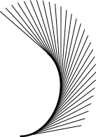
Figure 2: Edge of regression as envelope of the family of rulings

Since we may parametrise the developable surface as $g(t,\lambda)=\gamma(\lambda)+t\,\gamma^{\prime}(\lambda)$, the singular points of the surface satisfy

$$0=\frac{\partial g(t,\lambda)}{\partial t}\times\frac{\partial g(t,\lambda)}{\partial\lambda}=\gamma^{\prime}(\lambda)\times\left(\gamma^{\prime}(\lambda)+t\,\gamma^{\prime\prime}(\lambda)\right)=t\gamma^{\prime}(\lambda)\times\gamma^{\prime\prime}(\lambda),$$

and we notice that the edge of regression, if it exists, is part of the set of singular points of the developable surface.

Therefore, it is important to keep track of the edge of regression when modelling in order to avoid the appearance of undesired singularities.

Leaving out plane surfaces, which are trivially developable, we may classify developable surfaces according to their edge of regression into three families (see Fig. 3):

• Cylindrical surfaces: developable surfaces with no edge of regression at all. All rulings are parallel.

• Conical surfaces: developable surfaces for which the edge of regression is degenerate and reduces to a point, the vertex of the cone, where all rulings meet.

• Tangent surfaces: the generic case of a developable surface with an edge of regression which is an actual curve.

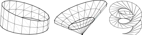
Figure 3: Classes of developable surfaces

The first two families are well understood within the NURBS formalism, are easy to construct and have therefore been used extensively in geometric modelling on resorting to developable surfaces. What it is aimed here is to produce a description of developable surfaces which may include the generic case of tangent surfaces.

3 Rational developable surfaces

In order to describe rational developable surfaces we start by considering a ruled surface interpolated between two rational curves of degree $n$, $c(t)$, $d(t)$, defined by their respective control polygons, $\{c_{0},\ldots,c_{n}\}$, $\{d_{0},\ldots,d_{n}\}$, and sets of weights $\{w_{0},\ldots,w_{n}\}$, $\{\omega_{0},\ldots,\omega_{n}\}$,

$$c(t)=\frac{\displaystyle\sum_{i=0}^{n}w_{i}c_{i}B^{n}_{i}(t)}{\displaystyle\sum_{i=0}^{n}w_{i}B^{n}_{i}(t)},\qquad d(t)=\frac{\displaystyle\sum_{i=0}^{n}\omega_{i}d_{i}B^{n}_{i}(t)}{\displaystyle\sum_{i=0}^{n}\omega_{i}B^{n}_{i}(t)},$$

in terms of the Bernstein polynomials of degree $n$, or the de Casteljau algorithm [28],

$$w^{r}_{i}(t) = (1-t)w^{r-1}_{i}(t)+tw^{r-1}_{i+1}(t),\quad i=0,\ldots,n-r,\quad r=1,\ldots,n,$$

$$c^{r}_{i}(t) = (1-t)\frac{w^{r-1}_{i}(t)}{w^{r}_{i}(t)}c^{r-1}_{i}(t)+t\frac{w^{r-1}_{i+1}}{w^{r}_{i}(t)}c^{r-1}_{i+1}(t),$$

$$c(t) := c^{n}_{0}(t)=(1-t)\frac{w^{n-1}_{0}(t)}{w^{n}_{0}(t)}c^{n-1}_{0}(t)+t\frac{w^{n-1}_{1}}{w^{n}_{0}(t)}c^{n-1}_{1}(t)$$ (2)

where $w^{0}_{i}=w_{i}$ and $c^{0}_{i}=c_{i}$.

From the derivatives of both numerator, $p(t)=w(t)c(t)$, and denominator of a rational curve $c(t)$,

$$p^{\prime}(t) = n\left(w^{n-1}_{1}(t)c^{n-1}_{1}(t)-w^{n-1}_{0}(t)c^{n-1}_{0}(t)\right),$$

$$w^{\prime}(t) = n\left(w^{n-1}_{1}(t)-w^{n-1}_{0}(t)\right),$$ (3)

we get the derivative of a rational curve $c(t)$ [29],

$$c^{\prime}(t)=\frac{p^{\prime}(t)-w^{\prime}(t)c(t)}{w(t)}=\frac{nw_{0}^{n-1}(t)w_{1}^{n-1}(t)}{w_{0}^{n}(t)^{2}}\left(c_{1}^{n-1}(t)-c_{0}^{n-1}(t)\right),$$

as a difference between the two last-but-one points in the de Casteljau algorithm.

Hence we have seen that the vectors $c^{\prime}(t)$, $d^{\prime}(t)$, $d(t)-c(t)$ are barycentric combinations of the points $c^{n-1}_{0}(t)$, $c^{n-1}_{1}(t)$, $d^{n-1}_{0}(t)$, $d^{n-1}_{1}(t)$. Therefore $c^{\prime}(t)$, $d^{\prime}(t)$, $d(t)-c(t)$ are coplanary if and only if $c^{n-1}_{0}(t)$, $c^{n-1}_{1}(t)$, $d^{n-1}_{0}(t)$, $d^{n-1}_{1}(t)$ lie on a plane and the developability condition (1) for a rational ruled surface may be restated in terms of these:

Proposition 3.1.

The ruled surface interpolating between two rational curves of degree $n$, defined by their respective control polygons, $\{c_{0},\ldots,c_{n}\}$, $\{d_{0},\ldots,d_{n}\}$, and sets of weights $\{w_{0},\ldots,w_{n}\}$, $\{\omega_{0},\ldots,\omega_{n}\}$, is developable if and only if the points $c^{n-1}_{0}(t)$, $c^{n-1}_{1}(t)$, $d^{n-1}_{0}(t)$, $d^{n-1}_{1}(t)$ are coplanary.

In order to avoid denominators, we may rewrite this result in terms of vectors in $\mathbb{R}^{4}$, $\mathbf{p}_{0}^{n-1}(t)$, $\mathbf{p}_{1}^{n-1}(t)$, $\mathbf{q}_{0}^{n-1}(t)$, $\mathbf{q}_{1}^{n-1}(t)$,

$$\mathbf{p}^{n-1}_{i}(t) = \left(w_{i}^{n-1}(t),w_{i}^{n-1}(t)c_{i}^{n-1}(t)\right),$$

$$\mathbf{q}^{n-1}_{i}(t) = \left(\omega_{i}^{n-1}(t),\omega_{i}^{n-1}(t)d_{i}^{n-1}(t)\right).$$

The condition of coplanarity for the points in affine space (Fig. 4) becomes a condition of linear dependence for the corresponding vectors in $\mathbb{R}^{4}$:

Corollary 3.2.

The ruled surface interpolating between two rational curves of degree $n$, defined by their respective control polygons, $\{c_{0},\ldots,c_{n}\}$, $\{d_{0},\ldots,d_{n}\}$, and sets of weights $\{w_{0},\ldots,w_{n}\}$, $\{\omega_{0},\ldots,\omega_{n}\}$, is developable if and only if the vectors $\mathbf{p}^{n-1}_{0}(t)$, $\mathbf{p}^{n-1}_{1}(t)$, $\mathbf{q}^{n-1}_{0}(t)$, $\mathbf{q}^{n-1}_{1}(t)$ are linearly dependent.

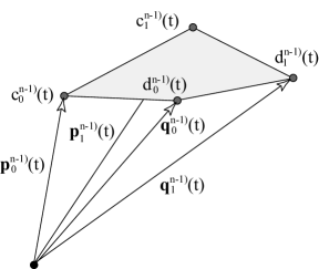
Figure 4: Points $c^{n-1}_{0}(t)$, $c^{n-1}_{1}(t)$, $c^{n-1}_{0}(t)$, $c^{n-1}_{1}(t)$ are coplanary iff vectors $\mathbf{p}^{n-1}_{0}(t)$, $\mathbf{p}^{n-1}_{1}(t)$, $\mathbf{q}^{n-1}_{0}(t)$, $\mathbf{q}^{n-1}_{1}(t)$ lie on a 3-space

That is, there exist rational coefficients $\lambda_{0}(t)$, $\lambda_{1}(t)$, $\mu_{0}(t)$, $\mu_{1}(t)$, such that

$$\lambda_{0}(t)\mathbf{p}^{n-1}_{0}(t)+\lambda_{1}(t)\mathbf{p}^{n-1}_{1}(t)=\mu_{0}(t)\mathbf{q}^{n-1}_{0}(t)+\mu_{1}(t)\mathbf{q}^{n-1}_{1}(t).$$

The coefficients in the equation are defined up to a multiplicative factor and we may divide it by $\lambda_{0}(t)+\lambda_{1}(t)$ and define $\Lambda(t)=\lambda_{1}(t)/\left(\lambda_{0}(t)+\lambda_{1}(t)\right)$, $M(t)=\mu_{1}(t)/\left(\mu_{0}(t)+\mu_{1}(t)\right)$, $\sigma(t)=\left(\mu_{0}(t)+\mu_{1}(t)\right)/\left(\lambda_{0}(t)+\lambda_{1}(t)\right)$,

$$\left(1-\Lambda(t)\right)\mathbf{p}^{n-1}_{0}(t)+\Lambda(t)\mathbf{p}^{n-1}_{1}(t)=\sigma(t)\left(\left(1-M(t)\right)\mathbf{q}_{0}^{n-1}(t)+M(t)\mathbf{q}_{1}^{n-1}(t)\right).$$ (4)

This way of writing the linear combination excludes the case of $\lambda_{1}=-\lambda_{0}$. However, it does not hinder our goal of coping with the generic case.

We may gain insight into this result by rewriting it in terms of blossoms,

$$\mathbf{p}^{1}_{i}[t_{1}] := \mathbf{p}^{1}_{i}(t_{1})=(1-t_{1})\mathbf{p}_{i}+t_{1}\mathbf{p}_{i+1},\quad i=0,\ldots,n-1,$$

$$\mathbf{p}^{r}_{i}[t_{1},\ldots,t_{r}] := (1-t_{r})\mathbf{p}_{i}^{r-1}[t_{1},\ldots,t_{r-1}]+t_{r}\mathbf{p}_{i+1}^{r-1}[t_{1},\ldots,t_{r-1}],$$

$$\mathbf{p}[t_{1},\ldots,t_{n}] := \mathbf{p}^{n}_{0}[t_{1},\ldots,t_{n}],\quad i=0,\ldots,n-r,\quad r=1,\ldots,n,$$ (5)

$$\mathbf{p}_{0}^{n-1}(t)=\mathbf{p}[t^{<n-1>},0],\quad\mathbf{p}_{1}^{n-1}(t)=\mathbf{p}[t^{<n-1>},1],\qquad t^{<a>}:=\underbrace{t,\ldots,t}_{a},$$

since linear combinations can be written in a rather compact form, taking into account that blossoms are multi-affine,

$$\mathbf{p}[t^{<n-1>},\Lambda(t)]=\sigma(t)\mathbf{q}[t^{<n-1>},M(t)].$$ (6)

We have therefore characterised developability of a generic rational ruled surface in terms of the polar forms of the bounding curves of the patch:

Theorem 3.3.

Two rational curves $c(t)$, $d(t)$ of degree $n$ with control polygons $\{c_{0},\ldots,c_{n}\}$, $\{d_{0},\ldots,d_{n}\}$ and weights $\{w_{0},\ldots,w_{n}\}$, $\{\omega_{0},\ldots,\omega_{n}\}$ define a generic developable surface if and only if there exist rational functions $\Lambda(t)$, $M(t)$, $\sigma(t)$ such that the blossoms of the curves in $\mathbb{R}^{4}$ are related by

$$\mathbf{p}[t^{<n-1>},\Lambda(t)]=\sigma(t)\mathbf{q}[t^{<n-1>},M(t)].$$

This expression is valid not just for rational Bézier curves, but also for rational spline curves, as it is done in [20] from Bézier to splines curves. The only difference between the Bézier and the spline cases is the expression of the blossom, which depends on the list of knots for splines.

$$\mathbf{p}^{1)}_{i}[t_{1}] := \mathbf{p}[u_{i+1},\ldots,u_{i+n-1},t_{1}]\;,$$

$$= \frac{u_{i+n}-t_{1}}{u_{i+n}-u_{i}}\mathbf{p}_{i}+\frac{t_{1}-u_{i}}{u_{i+n}-u_{i}}\mathbf{p}_{i+1}\;,\qquad i=0,\ldots,n-1\;,$$

$$\mathbf{p}^{r)}_{i}[t_{1},\ldots,t_{r}] := \mathbf{p}[u_{i+r},\ldots,u_{i+n-1},t_{1},\ldots,t_{r}]$$

$$= \frac{u_{i+n}-t_{r}}{u_{i+n}-u_{i+r-1}}\mathbf{p}^{r-1)}_{i}[t_{1},\ldots,t_{r-1}]$$

$$+ \frac{t_{r}-u_{i+r-1}}{u_{i+n}-u_{i+r-1}}\mathbf{p}^{r-1)}_{i+1}[t_{1},\ldots,t_{r-1}]\;,$$

$$i = 0,\ldots,n-r,\ r=1,\ldots,n\;,$$

$$\mathbf{p}[t_{1},\ldots,t_{n}] := \mathbf{p}^{n)}_{0}[t_{1},\ldots,t_{n}]=\frac{u_{n}-t_{n}}{u_{n}-u_{n-1}}\mathbf{p}^{n-1)}_{0}[t_{1},\ldots,t_{n-1}]$$

$$+ \frac{t_{n}-u_{n-1}}{u_{n}-u_{n-1}}\mathbf{p}^{n-1)}_{1}[t_{1},\ldots,t_{n-1}]\;,$$

$$\mathbf{p}(u) = \mathbf{p}[u,\ldots,u]:=\mathbf{p}[u^{<n>}]\;,$$

Theorem 3.4.

Two rational spline curves $c(t)$, $d(t)$ of degree $n$ and $N$ pieces, with respective control polygons $\{c_{0},\ldots,c_{n+N-1}\}$, $\{d_{0},\ldots,d_{n+N-1}\}$, weights $\{w_{0},\ldots,w_{n+N-1}\}$, $\{\omega_{0},\ldots,\omega_{n+N-1}\}$ and common list of knots $\{t_{0},\ldots,t_{2n+N-2}\}$ define a generic developable surface if and only if there exist rational functions $\Lambda(t)$, $M(t)$, $\sigma(t)$ such that the blossoms of the curves in $\mathbb{R}^{4}$ are related by

$$\mathbf{p}[t^{<n-1>},\Lambda(t)]=\sigma(t)\mathbf{q}[t^{<n-1>},M(t)].$$

We focus on rational developable surfaces from now on, since the extension to rational splines is seen to be straightforward.

4 Reparametrisation of rational ruled surfaces

There are two convenient alternative ways of parametrising rational ruled surfaces. If we have two rational curves of degree $n$ parametrised as $c(t)=p(t)/w(t)$, $d(t)=q(t)/\omega(t)$, the standard parametrisation would be

$$b(t,v)=(1-v)c(t)+vd(t),\qquad v\in[0,1].$$

The problem with this standard parametrisation of ruled surfaces in the rational case is that it is no longer of degree $n$ in $t$, since the denominators of the parametrisations $c(t)$ and $d(t)$ are different in general and hence $b(t,v)$ would be of degree $2n$.

A way of taking into account that we are dealing with rational parametrisations would be considering polynomial parametrisations in $\mathbb{R}^{4}$,

$$\mathbf{p}(t)=(w(t),p(t)),\qquad\mathbf{q}(t)=(\omega(t),q(t)).$$

We can consider the parametrisation for a polynomial ruled surface in $\mathbb{R}^{4}$ and project back to $\mathbb{R}^{3}$,

$$\tilde{b}(t,\tilde{v})=\frac{(1-\tilde{v})p(t)+\tilde{v}q(t)}{(1-\tilde{v})w(t)+\tilde{v}\omega(t)},\qquad\tilde{v}\in[0,1],$$ (7)

which is explicitly of degree $n$ in $t$.

Both parametrisations are related by a change of parameters

$$v=\frac{\tilde{v}\omega(t)}{(1-\tilde{v})w(t)+\tilde{v}\omega(t)}.$$

From now on we use (7) as our standard parametrisation for rational ruled surfaces, omitting the tilde for $v$ and $b$.

This result is useful for interpreting the functions $\Lambda$, $M$, $\sigma$:

Except for the case of cylindrical developable surfaces, another way of expressing that the tangent plane to a developable surface is the same at all points on the same ruling [27] is the requirement of the existence of two functions $\lambda(t)$, $\mu(t)$ such that

$$c^{\prime}(t)=\lambda(t)\textbf{w}(t)+\mu(t)\mathbf{w}^{\prime}(t),\qquad\mathbf{w}(t):=d(t)-c(t).$$ (8)

We can use the previous result on parametrisations of ruled surfaces and rewrite this condition for parametrisations in $\mathbb{R}^{4}$ for rational ruled surfaces in $\mathbb{R}^{3}$,

$$\mathbf{p}^{\prime}(t)=\lambda(t)\textbf{W}(t)+\mu(t)\mathbf{W}^{\prime}(t)+\nu(t)\textbf{p}(t),\qquad\mathbf{W}(t):=\mathbf{q}(t)-\mathbf{p}(t),$$ (9)

allowing for an extra term along $\mathbf{p}(t)$ which vanishes on proyecting back from $\mathbb{R}^{4}$ to $\mathbb{R}^{3}$.

This term may be removed by the introduction of a suitable global factor $f(t)$,

$$\mathbf{\tilde{p}}(t)=f(t)\mathbf{p}(t),\qquad\mathbf{\tilde{q}}(t)=f(t)\mathbf{q}(t),$$

$$\mathbf{\tilde{p}}^{\prime}(t) = f(t)\mathbf{p}^{\prime}(t)+f^{\prime}(t)\mathbf{p}(t)=\left(\lambda(t)-\mu(t)\frac{f^{\prime}(t)}{f(t)}\right)\mathbf{\tilde{W}}(t)+\mu(t)\mathbf{\tilde{W}}^{\prime}(t)+\left(\nu(t)+\frac{f^{\prime}(t)}{f(t)}\right)\mathbf{\tilde{p}}(t)$$

$$= \tilde{\lambda}(t)\mathbf{\tilde{W}}(t)+\tilde{\mu}(t)\mathbf{\tilde{W}}^{\prime}(t)+\tilde{\nu}(t)\mathbf{\tilde{p}}(t),$$

from which we can read the terms of the new decomposition,

$$\tilde{\lambda}(t)=\lambda(t)-\mu(t)\frac{f^{\prime}(t)}{f(t)},\quad\tilde{\mu}(t)=\mu(t),\quad\tilde{\nu}(t)=\nu(t)+\frac{f^{\prime}(t)}{f(t)},$$

and infer that the $\nu$ term can be cancelled by choosing

$$f(t)=e^{-\int\nu(t)\,dt}.$$

We can relate these functions $\lambda,\mu,\nu$ with the ones we have introduced in Theorem 3.3, using blossom expressions for $\mathbf{p}$, $\mathbf{p}^{\prime}$ and $\mathbf{q}$,

$$\textbf{p}(t)=(1-t)\mathbf{p}[t^{<n-1>},0]+t\mathbf{p}[t^{<n-1>},1],$$

$$\textbf{q}(t)=(1-t)\mathbf{q}[t^{<n-1>},0]+t\mathbf{q}[t^{<n-1>},1],$$

$$\mathbf{p}^{\prime}(t)=n\mathbf{p}[t^{<n-1>},1]-n\mathbf{p}[t^{<n-1>},0],$$

$$\mathbf{q}^{\prime}(t)=n\mathbf{q}[t^{<n-1>},1]-n\mathbf{q}[t^{<n-1>},0],$$ (10)

and grouping terms in (9),

$$\mathbf{p}[t^{<n-1>},1]\left(n(1+\mu(t))+t(\lambda(t)-\nu(t))\right)$$

$$+ \mathbf{p}[t^{<n-1>},0]\left((1-t)(\lambda(t)-\nu(t))-n(1+\mu(t))\right)$$

$$= \mathbf{q}[t^{<n-1>},1]\left(\lambda(t)t+n\mu(t)\right)+\mathbf{q}[t^{<n-1>},0]\left(\lambda(t)(1-t)-n\mu(t)\right)$$

we read from Theorem 3.3:

Corollary 4.1.

For a rational developable surface bounded by rational curves of degree $n$, the functions $\Lambda$, $M$, $\sigma$ in Theorem 3.3 are given by

$$\Lambda(t)=\frac{n\left(\mu(t)+1\right)+\left(\lambda(t)-\nu(t)\right)t}{\lambda(t)-\nu(t)},\ M(t)=\frac{\lambda(t)t+n\mu(t)}{\lambda(t)},\ \sigma(t)=\frac{\lambda(t)}{\lambda(t)-\nu(t)},$$

$$\lambda(t)=\frac{n\sigma(t)}{\Lambda(t)-\sigma(t)M(t)+t\left(\sigma(t)-1\right)},\ \mu(t)=\frac{\sigma(t)\left(M(t)-t\right)}{\Lambda(t)-\sigma(t)M(t)+t\left(\sigma(t)-1\right)},$$

$$\nu(t)=\frac{n\left(\sigma(t)-1\right)}{\Lambda(t)-\sigma(t)M(t)+t\left(\sigma(t)-1\right)},$$

in terms of the ones in the expansion (9) for parametrisations $\mathbf{p}(t)$, $\mathbf{q}(t)$ in $\mathbb{R}^{4}$ of the rational curves.

In this sense, Theorem 3.3 just expresses an alternative way of writing the rational version (9) of the standard decomposition (8) for rational Bézier curves.

As expected, when $\nu\equiv 0$, no term along the projection direction appears and then $\sigma\equiv 1$. In this case, we recover the results for Bézier developable surfaces [19].

These relations are useful for linking results in both formalisms for rational developable surfaces.

5 Features of rational developable surfaces

We check now how most common operations with rational curves affect rational developables surfaces:

• Multiplication of weights by a constant: If we multiply the weights of a rational curve by a constant, the parametrisation does not change.

  If we multiply the list of weights of both bounding rational curves respectively by constants $\alpha$, $\beta$, so that the new lists are $\{\alpha w_{0},\ldots,\alpha w_{n}\}$, $\{\beta\omega_{0},\ldots,\beta\omega_{n}\}$,

  $$\frac{\mathbf{p}[t^{<n-1>},\Lambda(t)]}{\alpha}=\sigma(t)\frac{\mathbf{q}[t^{<n-1>},M(t)]}{\beta},$$

  it is clear that the functions $\Lambda(t)$, $M(t)$ do not change but $\sigma(t)$ changes to $\alpha\sigma(t)/\beta$.

• Reparametrisation under Möbius transformations [30, 28]: Möbius transformations of the interval $[0,1]$ onto itself,

  $$t(u)=\frac{u}{(1-b)u+b},\quad u\in[0,1],$$ (11)

  are equivalent to a change of the lists of weights $\{\tilde{w}_{0},\ldots,\tilde{w}_{n}\}$, $\{\tilde{\omega}_{0},\ldots,\tilde{\omega}_{n}\}$, $\tilde{w}_{i}=b^{n-i}w_{i}$, $\tilde{\omega}_{i}=b^{n-i}\omega_{i}$, $i=0,\ldots,n$, while keeping the same control polygons for the curves.

  Since we may relate both polar forms by

  $$\frac{\mathbf{\tilde{p}}[u^{<n-1>},\tilde{\Lambda}(u)]}{\left((1-b)u+b\right)^{n-1}(1-b)\tilde{\Lambda}(u)+b} = \mathbf{p}\left[\left.\frac{u}{(1-b)u+b}\right.^{<n-1>},\frac{\tilde{\Lambda}(u)}{(1-b)\tilde{\Lambda}(u)+b}\right]$$

  $$= \mathbf{p}\left[t(u)^{<n-1>},\frac{\tilde{\Lambda}(u)}{(1-b)\tilde{\Lambda}(u)+b}\right],$$

  we can write the developabity condition in terms of $\mathbf{\tilde{p}}$ and $\mathbf{\tilde{q}}$,

  $$\mathbf{p}[u^{<n-1>},\tilde{\Lambda}(u)]=\tilde{\sigma}(u)\mathbf{q}[u^{<n-1>},\tilde{M}(u)],$$

  for some new functions $\tilde{\Lambda}(u)$, $\tilde{M}(u)$, $\tilde{\sigma}(u)$, which we may relate to the previous ones,

  $$\left((1-b)\tilde{\Lambda}(u)+b\right)\mathbf{p}\left[t(u)^{<n-1>},\frac{\tilde{\Lambda}(u)}{(1-b)\tilde{\Lambda}(u)+b}\right]=\frac{\mathbf{\tilde{p}}[u^{<n-1>},\tilde{\Lambda}(u)]}{\left((1-b)u+b\right)^{n-1}}$$

  $$=\tilde{\sigma}(u)\frac{\mathbf{\tilde{q}}[u^{<n-1>},\tilde{M}(u)]}{\left((1-b)u+b\right)^{n-1}}=\tilde{\sigma}(u)\left((1-b)\tilde{M}(u)+b\right)\mathbf{q}\left[t(u)^{<n-1>},\frac{\tilde{M}(u)}{(1-b)\tilde{M}(u)+b}\right]$$

  and comparing with the developability condition in terms of $\mathbf{p}$ and $\mathbf{q}$, we get

  $$\Lambda(t(u))=\frac{\tilde{\Lambda}(u)}{(1-b)\tilde{\Lambda}(u)+b},\quad M(t(u))=\frac{\tilde{M}(u)}{(1-b)\tilde{M}(u)+b},\quad\sigma(t(u))=\tilde{\sigma}(u)\frac{(1-b)\tilde{M}(u)+b}{(1-b)\tilde{\Lambda}(u)+b},$$

  $$\tilde{\Lambda}(u)=\frac{b\Lambda(t(u))}{1+(b-1)\Lambda(t(u))},\quad\tilde{M}(u)=\frac{bM(t(u))}{1+(b-1)M(t(u))},\quad\tilde{\sigma}(u)=\sigma(t(u))\frac{1+(b-1)M(t(u))}{1+(b-1)\Lambda(t(u))}.$$ (12)

  We notice that in both cases a non-trivial $\sigma$ arises even if in the original parametrisation $\sigma$ is one.

• Degree elevation: We may formally increase the degree of the parametrisations by multiplicating $\mathbf{p}$ and $\mathbf{q}$ by respective factors $f(t)$, $g(t)$ of degree one, which cancel out on projecting to $\mathbb{R}^{3}$. The new parametrisations are $\mathbf{\tilde{p}}=f\mathbf{p}$ and $\mathbf{\tilde{q}}=g\mathbf{q}$ of degree $n+1$.

  In order to compute the functions $\tilde{\Lambda}$, $\tilde{M}$ and $\tilde{\sigma}$ for the degree-elevated parametrisations we compute, developing the blossom expressions,

  $$\mathbf{\tilde{p}}[t^{<n>},\tilde{\Lambda}(t)] = \frac{nf(t)\mathbf{p}[t^{<n-1>},\tilde{\Lambda}(t)]+f(\tilde{\Lambda}(t))\mathbf{p}[t^{<n>}]}{n+1}$$

  $$= \frac{n(1-\tilde{\Lambda}(t))f(t)+f(\tilde{\Lambda}(t))(1-t)}{n+1}\mathbf{p}^{n-1}_{0}(t)$$

  $$+ \frac{n\tilde{\Lambda}(t)f(t)+f(\tilde{\Lambda}(t))t}{n+1}\mathbf{p}^{n-1}_{1}(t),$$

  $$\mathbf{\tilde{q}}[t^{<n>},\tilde{M}(t)] = \frac{ng(t)\mathbf{q}[t^{<n-1>},\tilde{M}(t)]+g(\tilde{M}(t))\mathbf{q}[t^{<n>}]}{n+1}$$

  $$= \frac{n(1-\tilde{M}(t))g(t)+g(\tilde{M}(t))(1-t)}{n+1}\mathbf{q}^{n-1}_{0}(t)$$

  $$+ \frac{n\tilde{M}(t)g(t)+g(\tilde{M}(t))t}{n+1}\mathbf{q}^{n-1}_{1}(t),$$

  and comparing them with the developability condition for the original parametrisations

  $$(1-\Lambda(t))\mathbf{p}_{0}(t)+\Lambda(t)\mathbf{p}_{1}(t)=\sigma(t)\left((1-M(t))\mathbf{q}_{0}(t)+M(t)\mathbf{q}_{1}(t)\right),$$

  we read

  $$\Lambda(t)=\frac{nf(t)\tilde{\Lambda}(t)+f(\tilde{\Lambda}(t))t}{nf(t)+f(\tilde{\Lambda}(t))},\quad M(t)=\frac{ng(t)\tilde{M}(t)+g(\tilde{M}(t))t}{ng(t)+g(\tilde{M}(t))},\quad\sigma(t)=\frac{ng(t)+g(\tilde{M}(t))}{nf(t)+f(\tilde{\Lambda}(t))}\tilde{\sigma}(t).$$ (13)

  The simplest case for degree elevation is the one with $f\equiv 1\equiv g$,

  $$\Lambda(t)=\frac{n\tilde{\Lambda}(t)+t}{n+1},\quad M(t)=\frac{n\tilde{M}(t)+t}{n+1},\quad\sigma(t)=\tilde{\sigma}(t),$$

  which is the same that was found for Bézier developable surfaces.

• Modification of the lengths of the rulings: We may change the endpoints of the rulings of a developable surface patch bounded by two rational curves $c(t)$, $d(t)$ of degree $n$ by modifying the length of the vector $\mathbf{q}(t)-\mathbf{p}(t)$ by a linear factor $g(t)$ as in [18], $g(t)\left(\mathbf{q}(t)-\mathbf{p}(t)\right)$.

  Since all terms are of degree $n+1$ but $\mathbf{p}(t)$, we may even allow for degree elevation of the form $f(t)\mathbf{p}(t)$, where $f(t)$ is a factor of degree one,

  $$\mathbf{\tilde{p}}(t)=f(t)\mathbf{p}(t),\qquad\mathbf{\tilde{q}}(t)=f(t)\mathbf{p}(t)+g(t)\left(\mathbf{q}(t)-\mathbf{p}(t)\right),$$

  parametrisations which are related by the developabilty condition,

  $$\mathbf{\tilde{p}}[t^{<n>},\tilde{\Lambda}(t)]=\tilde{\sigma}(t)\mathbf{\tilde{q}}[t^{<n>},\tilde{\Lambda}(t)],$$

  for some rational functions $\tilde{\Lambda}(t)$, $\tilde{M}(t)$, $\tilde{\sigma}(t)$.

  Expanding these expressions,

  $$\mathbf{\tilde{p}}[t^{<n>},\tilde{\Lambda}(t)]=\frac{f(\tilde{\Lambda}(t))\mathbf{p}[t^{<n>}]+nf(t)\mathbf{p}[t^{<n-1>},\tilde{\Lambda}(t)]}{n+1},$$

  $$\mathbf{\tilde{q}}[t^{<n>},\tilde{M}(t)] = \frac{f(\tilde{M}(t))\mathbf{p}[t^{<n>}]+nf(t)\mathbf{p}[t^{<n-1>},\tilde{M}(t)]}{n+1}$$

  $$+ \frac{g(\tilde{M}(t))\mathbf{q}[t^{<n>}]+ng(t)\mathbf{q}[t^{<n-1>},\tilde{M}(t)]}{n+1}$$

  $$- \frac{g(\tilde{M}(t))\mathbf{p}[t^{<n>}]+ng(t)\mathbf{p}[t^{<n-1>},\tilde{M}(t)]}{n+1},$$

  and comparing them with

  $$\mathbf{p}[t^{<n>},\Lambda(t)]=\sigma(t)\mathbf{q}[t^{<n>},\Lambda(t)],$$

  we get the relations between both sets of functions,

  $$\Lambda(t) = \frac{f(\tilde{\Lambda}(t))t+nf(t)\tilde{\Lambda}(t)+\tilde{\sigma}(t)\left(n\tilde{M}(t)\left(g(t)-f(t)\right)+t\left(g(\tilde{M}(t))-f(\tilde{M}(t))\right)\right)}{f(\tilde{\Lambda}(t))+nf(t)+\tilde{\sigma}(t)\left(g(\tilde{M}(t))-f(\tilde{M}(t))+n\left(g(t)-f(t)\right)\right)},$$

  $$M(t) = \frac{g(\tilde{M}(t))t+ng(t)\tilde{M}(t)}{g(\tilde{M}(t))+ng(t)},$$

  $$\sigma(t) = \tilde{\sigma}(t)\frac{g(\tilde{M}(t))+ng(t)}{f(\tilde{\Lambda}(t))+nf(t)+\tilde{\sigma}(t)\left(g(\tilde{M}(t))-f(\tilde{M}(t))+n\left(g(t)-f(t)\right)\right)}.$$ (14)

  In the case $f\equiv g$, we recover the expressions obtained for degree elevation with the same factor, since the rulings do not change.

  Another simple case is the one with $\sigma\equiv 1\equiv f$, that is, with modification of the global factor just for $\mathbf{q}-\mathbf{p}$,

  $$\Lambda(t)=\frac{n\tilde{\Lambda}(t)+\left(n\tilde{M}(t)\left(g(t)-1\right)+tg(\tilde{M}(t))\right)}{g(\tilde{M}(t))+ng(t)},$$

  $$M(t)=\frac{g(\tilde{M}(t))t+ng(t)\tilde{M}(t)}{g(\tilde{M}(t))+ng(t)},\qquad\sigma\tilde{\equiv}1.$$

• Knot insertion: One of the advantages of writing the developability condition in terms of blossoms is the invariance under knot insertion. That is, if we insert a new knot in the list, the expressions for $\Lambda$, $M$ and $\sigma$ will not change.

6 Edge of regression

The edge of regression is the set of points of the developable surface where the surface is singular. The coordinate patch $(t,v)$ fails at the edge, since the vectors $b_{t}$ and $b_{v}$ are parallel. The developable surface can be seen as the tangent surface to its edge of regression [27], except for the cases of cylindrical and conical surfaces.

We may compute the edge of regression of a rational developable surface, making use of the polynomial parametrisations of the bounding curves, $\mathbf{p}(t)$ and $\mathbf{q}(t)$ in $\mathbb{R}^{4}$.

Before projection onto $\mathbb{R}^{3}$, the polynomial parametrisation would be

$$\textbf{b}(t,v)=(1-v)\mathbf{p}(t)+v\mathbf{q}(t),$$

but in this case we cannot simply require parallelism, $\mathbf{b}_{t}=\alpha\mathbf{b}_{v}$, of the derivatives

$$\mathbf{b}_{t}(t,v)=(1-v)\mathbf{p}^{\prime}(t)+v\mathbf{q}^{\prime}(t),\qquad\mathbf{b}_{v}=\mathbf{q}(t)-\mathbf{p}(t),$$

but allow an additional term along $\mathbf{b}$ which vanishes on projecting to $\mathbb{R}^{3}$,

$$(1-v)\mathbf{p}^{\prime}(t)+v\mathbf{q}^{\prime}(t)=\alpha(t,v)\left(\mathbf{q}(t)-\mathbf{p}(t)\right)+\beta(t,v)\left((1-v)\mathbf{p}(t)+v\mathbf{q}(t)\right)$$

Following (4), we may group terms in the previous expression,

$$\mathbf{p}[t^{<n-1>},0]\left(n(v-1)+(1-t)\left(\alpha(t,v)+(v-1)\beta(t,v)\right)\right)$$

$$+ \mathbf{p}[t^{<n-1>},1]\left(n(1-v)+t\left(\alpha(t,v)+(v-1)\beta(t,v)\right)\right)$$

$$= \mathbf{q}[t^{<n-1>},0]\left(nv+(1-t)\left(\alpha(t,v)+v\beta(t,v)\right)\right)$$

$$+ \mathbf{q}[t^{<n-1>},1]\left(-nv+t\left(\alpha(t,v)+v\beta(t,v)\right)\right),$$

and compare them with the ones in Theorem 3.3 to yield

$$\Lambda(t)=t+\frac{n(1-v)}{\alpha(t,v)+(v-1)\beta(t,v)},\quad M(t)=t-\frac{nv}{\alpha(t,v)+v\beta(t,v)},$$

$$\sigma(t)=\frac{\alpha(t,v)+v\beta(t,v)}{\alpha(t,v)+(v-1)\beta(t,v)},$$

from which we can eliminate $\alpha$ and $\beta$, which happen not to depend on $v$,

$$\alpha(t)=\frac{n\sigma(t)\left(\Lambda(t)-M(t)\right)}{\left(\Lambda(t)-t+\sigma(t)\left(t-M(t)\right)\right)^{2}},\quad\beta(t)=\frac{n\left(\sigma(t)-1\right)}{\Lambda(t)-t+\sigma(t)\left(t-M(t)\right)},$$

and we obtain a parametrisation of the edge of regression:

Corollary 6.1.

A rational developable surface with bounding curves $c(t)$, $d(t)$ satisfying

$$\mathbf{p}[t^{<n-1>},\Lambda(t)]=\sigma(t)\mathbf{q}[t^{<n-1>},M(t)],$$

for some rational functions $\Lambda$, $M$, $\sigma$ has a rational edge of regression parametrised in $\mathbb{R}^{4}$ by

$$\textbf{r}(t)=(1-v(t))\mathbf{p}(t)+v(t)\mathbf{q}(t),\qquad v(t)=\frac{\sigma(t)\left(t-M(t)\right)}{\Lambda(t)-t+\sigma(t)\left(t-M(t)\right)}.$$ (15)

We notice that in the case of constant $\Lambda$, $M$, $\sigma$, the edge of regression is a rational curve of degree $n+1$, since the parametric equation $v(t)$ is of degree one.

Hence, developable surfaces bounded by rational curves of degree $n$ with constant functions $\Lambda$, $M$, $\sigma$ have rational edges of regression of degree $n+1$.

We may check if the converse is also true. That is, if all rational developable surfaces with rational edge of regression of degree $n$ have surface patches of degree $(n-1,1)$ with constant functions $\Lambda$, $M$, $\sigma$:

The simplest generic developable surface is the tangent surface to a curve $\textbf{r}(t)$ of degree $n$, which is the edge of regression of the developable surface,

$$\mathbf{b}(t,v)=\mathbf{r}(t)+vf(t)\mathbf{r}^{\prime}(t),$$

which is a rational developable surface patch of degree $(n,1)$ provided that the factor $f$ is linear, $f(t)=at+b$.

According to (9), $\mathbf{r}^{\prime}(t)=\mathbf{W}(t)/f(t)$ and hence $\lambda(t)=1/f(t)$, $\mu(t)=0$, $\nu(t)=0$, so that

$$\Lambda(t)=t+nf(t),\qquad M(t)=t,\qquad\sigma\equiv 1.$$

We may choose another surface patch bounded by two curves of degree $n-1$ on the developable surface, since it is clear that if we take $v=1$, $a=-1/n$ on the parametrisation, all resulting curves, depending on $b$, are of degree $n-1$, since we have removed the leading term in $t$ in their parametrisations.

With the following choice of the free parameter $b$,

$$\mathbf{p}(t)=\mathbf{r}(t)+\frac{M-t}{n}\mathbf{r}^{\prime}(t),\qquad\mathbf{q}(t)=\mathbf{r}(t)+\frac{\Lambda-t}{n}\mathbf{r}^{\prime}(t),$$

it is easy to check that the developable surface patch bounded by the respective curves $c(t)$ and $d(t)$ of degree $n-1$ has constant functions $\Lambda$, $M$, $\sigma=1$:

Theorem 6.2.

The set of developable surfaces with patches generated by two rational curves $c(t)$, $d(t)$ of degree $n$, with ruling generators $\mathbf{q}(t)-\mathbf{p}(t)$ also of degree $n$ and blossoms related by

$$\mathbf{p}[t^{<n-1>},\Lambda]=\mathbf{q}[t^{<n-1>},M],$$

with constant $\Lambda$, $M$, $\sigma=1$, is the set of tangent surfaces to rational curves of degree $n+1$.

That is, we may generate the rational developable surfaces with constant $\Lambda$, $M$, $\sigma=1$ patches and then adapt these patches.

The proof is simple, writing (9) in our case,

$$\mathbf{W}(t)=\mathbf{q}(t)-\mathbf{p}(t)=\frac{\Lambda-M}{n}\mathbf{r}^{\prime}(t),\qquad\mathbf{W}^{\prime}(t)=\frac{\Lambda-M}{n}\mathbf{r}^{\prime\prime}(t),$$

$$\lambda(t)\mathbf{W}(t)+\mu(t)\mathbf{W}^{\prime}(t)=\mathbf{p}^{\prime}(t)=\mathbf{r}^{\prime}(t)-\frac{\mathbf{r}^{\prime}(t)}{n}+\frac{M-t}{n}\mathbf{r}^{\prime\prime}(t)=\frac{n-1}{\Lambda-M}\mathbf{W}(t)+\frac{M-t}{\Lambda-M}\mathbf{W}^{\prime}(t),$$

from which we read the functions $\lambda(t)$, $\mu(t)$, $\nu(t)$,

$$\lambda(t)=\frac{n-1}{\Lambda-M},\qquad\mu(t)=\frac{M-t}{\Lambda-M},\qquad\nu(t)=0,$$

which correspond to the right values of $\Lambda$, $M$, $\sigma$, according to Corollary 2, for $c(t)$ of degree $n-1$.

7 The constant $\Lambda$, $M$, $\sigma$ case

The simplest case which can be considered is the one with constant coefficients $\Lambda$, $M$, $\sigma$,

$$\mathbf{p}[t^{<n-1>},\Lambda]=\sigma\mathbf{q}[t^{<n-1>},M].$$

This expression states the equality of two $(n-1)$-atic forms, which is equivalent to the equality of the respective symmetric $(n-1)$-affine forms, since the correspondence between blossoms and parametrizations is one-to-one,

$$\mathbf{p}[t_{1},\ldots,t_{n-1},\Lambda]=\sigma\mathbf{q}[t_{1},\ldots,t_{n-1},M]\ .$$ (16)

We may draw information about the control net applying it to sequences of zeros and ones, taking into account that the vertices are recovered as

$$\mathbf{p}_{j}=\mathbf{p}[0^{<n-j>},1^{<j>}],$$

$$(1-\Lambda)\mathbf{p}_{j}+\Lambda\mathbf{p}_{j+1}=(1-M)\sigma\mathbf{q}_{j}+M\sigma\mathbf{q}_{j+1},\quad j=0,\ldots,n-1,$$

stating that the cells of the control net of the surface in $\mathbb{R}^{4}$ are planar and share the same linear combination of vertices.

Projecting back into affine space, we get the relation between weights and vertices of the control net,

$$(1-\Lambda)w_{j}+\Lambda w_{j+1}=(1-M)\sigma\omega_{j}+M\sigma\omega_{j+1},$$

$$(1-\Lambda)w_{j}c_{j}+\Lambda w_{j+1}c_{j+1}=(1-M)\sigma\omega_{j}d_{j}+M\sigma\omega_{j+1}d_{j+1}.$$

This can be considered the natural generalization of Aumann’s result for Bézier developable surfaces to the rational case [17], though in that paper the key issue was the use of an affine transformation between adjacent cells of the control net of the surface.

8 Example

We construct the rational developable surface bounded by a curve $c(t)$ with control polygon $\{(0,0,0),(3,3,0),(4,3,0),(5,0,0)\}$ and weights $\{1,1,3/5,5/6\}$ and a curve $d(t)$ with $d_{0}=(0,0,2)$, $d_{1}=(2,2,3)$, $\omega_{0}=1$, $\omega_{1}=1$.

Figure 5: Developable surface bounded by rational cubic curves

We complete the control polygon,

$$\{(0,0,2),(2,2,3),(3/2,21/22,135/22),(293/172,-189/172,1215/172)\},$$

and list of weights of $d(t)$,

$$\{1,1,11/15,43/45\},$$

building a patch with constant $\Lambda,M,\sigma$ as in Section 7, for which $\Lambda=-4/3$, $M=-2$, $\sigma=1$. The resulting developable surface is shown in Fig. 5.

The edge of regression is the curve parametrised by

$$r(t)=(1-v(t))c(t)+v(t)d(t),\qquad v(t)=\frac{\sigma(t-M)}{\Lambda-t+\sigma(t-M)}=\frac{3}{2}t+3,$$

according to corollary 3.

If we perform a Möbius transformation (11) with $b=2$ on both bounding curves, so that the respective new sets of weights are $\{8,4,6/5,5/6\}$ and $\{8,4,22/15,43/45\}$, the new parametrisation for the developable surface has new constants given by (12),

$$\tilde{\Lambda}=\frac{b\Lambda}{1+(b-1)\Lambda}=8,\quad\tilde{M}=\frac{bM}{1+(b-1)M}=4,\quad\tilde{\sigma}=\sigma\frac{1+(b-1)M}{1+(b-1)\Lambda}=3.$$

If we raise the degree of both curves in the usual way, with $f\equiv 1\equiv g$, the control polygons of the curves change to (see Fig. 6)

$$\{(0,0,0),(9/4,9/4,0),(27/8,3,0),(341/79,162/79,0),(5,0,0)\},$$

$$\{(0,0,2),(3/2,3/2,11/4),(93/52,81/52,225/52),(887/568,189/568,3645/568),(293/172,-189/172,1215/172)\},$$

and the lists of weights to $\{1,1,4/5,79/120,5/6\}$, $\{1,1,13/15,71/90,43/45\}$. According to (13), the new functions are

$$\tilde{\Lambda}(u)=-\frac{u}{3}-\frac{16}{9},\qquad\tilde{M}(u)=-\frac{u}{3}-\frac{8}{3},\qquad\tilde{\sigma}(u)=1.$$

Figure 6: Degree-elevated developable surface patch

We may shorten the lengths of the rulings of our patch, since the last ruling is much larger than the first one. For instance, we may move the boundary of the patch from $d(t)$ to $\tilde{d}(t)=c(t)+g(t)(d(t)-c(t))$. If we take $g(t)=1-3t/4$, we get, according to (• ‣ 5),

$$\tilde{\Lambda}(t)=\frac{1}{9}\frac{9t^{2}-3t-32}{1-2t},\quad M(t)=\frac{1}{3}\frac{7t-16}{1-2t},\quad\sigma(t)=1,$$

since we have not introduced a global factor $f(t)$ for $c(t)$. The result may be seen in Fig. 7.

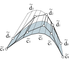
Figure 7: Trimmed developable surface patch

Finally, we consider our surface patch as a spline patch of one piece with trivial lists of knots, $\{0,0,0,1,1,1\}$, and $\{0,1\}$. If we insert a new knot $t=2/3$ (see Fig. 8), $\Lambda$, $M$, $\sigma$ do not change.

Figure 8: Knot-inserted developable surface patch

9 Conclusions

In this paper a new characterization of rational and NURBS developable surfaces in terms of blossoms of their bounding curves has been produced. This is useful for CAD purposes, since the bounding curves are described in terms of their control points, weights and knots. As a consequence, a way of constructing generic rational developable surfaces has been shown, using linear relations between the control points and weights of the cells of the control net of the surface. This construction is compatible with algorithms based on blossoms and allows easily elevation of degree. The edge of regression of the developable surface has a simple expression in terms of the parameters used for deriving the construction.

References

• [1] M. Perriollat, A. Bartoli, A computational model of bounded developable surfaces with application to image-based three-dimensional reconstruction, Computer Animation & Virtual Worlds 24 (5) (2013) 459–476. doi:10.1002/cav.1478.
• [2] H. Pottmann, A. Asperl, M. Hofer, A. Kilian, Architectural geometry, Bentley Institute Press, Exton, 2007.
• [3] K. Rose, A. Sheffer, J. Wither, M.-P. Cani, B. Thibert, Developable surfaces from arbitrary sketched boundaries, in: A. Belyaev, M. Garland (Eds.), Eurographics Symposium on Geometry Processing (2007), The Eurographics Association, 2007, pp. 163–172.
• [4] U. Kilgore, Developable hull surfaces, in: Fishing Boats of the World, Vol. 3, Fishing News Books Ltd., Surrey, 1967, pp. 425–431.
• [5] J. S. Chalfant, T. Maekawa, Design for manufacturing using B-spline developable surfaces., J. Ship Research 42 (3) (1998) 207–215.
• [6] F. Pérez, J. Suárez, Quasi-developable B-spline surfaces in ship hull design, Computer-Aided Design 39 (10) (2007) 853–862. doi:10.1016/j.cad.2007.04.004.
• [7] W. H. Frey, D. Bindschadler, Computer aided design of a class of developable Bézier surfaces, Tech. rep., GM Research Publication R&D-8057 (1993).
• [8] H. Pottmann, J. Wallner, Computational line geometry, Mathematics and Visualization, Springer-Verlag, Berlin, 2001.
• [9] J. Lang, O. Röschel, Developable $(1,n)$-Bézier surfaces, Comput. Aided Geom. Design 9 (4) (1992) 291–298. doi:10.1016/0167-8396(92)90036-O.
• [10] G. Aumann, Interpolation with developable Bézier patches, Comput. Aided Geom. Design 8 (5) (1991) 409–420.
• [11] T. Maekawa, Design and tessellation of B-spline developable surfaces, ASME Transactions Journal of Mechanical Design 120 (1998) 453–461.
• [12] R. M. C. Bodduluri, B. Ravani, Design of developable surfaces using duality between plane and point geometries., Computer Aided Design 25 (10) (1993) 621–632.
• [13] H. Pottmann, G. Farin, Developable rational Bézier and $B$-spline surfaces, Comput. Aided Geom. Design 12 (5) (1995) 513–531.
• [14] H. Pottmann, J. Wallner, Approximation algorithms for developable surfaces, Comput. Aided Geom. Design 16 (6) (1999) 539–556.
• [15] C. Tang, P. Bo, J. Wallner, H. Pottmann, Interactive design of developable surfaces, ACM Trans. Graph. 35 (2) (2016) 12:1–12:12.
• [16] C.-H. Chu, C. H. Séquin, Developable Bézier patches: properties and design, Computer Aided Design 34 (7) (2002) 511–527.
• [17] G. Aumann, A simple algorithm for designing developable Bézier surfaces, Comput. Aided Geom. Design 20 (8-9) (2003) 601–619, in memory of Professor J. Hoschek.
• [18] G. Aumann, Degree elevation and developable Bézier surfaces, Comput. Aided Geom. Design 21 (7) (2004) 661–670.
• [19] L. Fernández-Jambrina, Bézier developable surfaces, Comput. Aided Geom. Design 55 (2017) 15–28. doi:10.1016/j.cagd.2017.02.001.
• [20] L. Fernández-Jambrina, B-spline control nets for developable surfaces, Comput. Aided Geom. Design 24 (4) (2007) 189–199. doi:10.1016/j.cagd.2007.03.001.
• [21] A. Cantón, Fernández-Jambrina, Interpolation of a spline developable surface between a curve and two rulings, Frontiers of Information Technology & Electronic Engineering 16 (2015) 173–190.
• [22] A. Cantón, L. Fernández-Jambrina, Non-degenerate developable triangular Bézier patches, in: J.-D. Boissonnat, P. Chenin, A. Cohen, C. Gout, T. Lyche, M.-L. Mazure, L. Schumaker (Eds.), Curves and Surfaces, Vol. 6920 of Lecture Notes in Computer Science, Springer Berlin / Heidelberg, 2012, pp. 207–219.
• [23] S. Leopoldseder, Algorithms on cone spline surfaces and spatial osculating arc splines, Comput. Aided Geom. Des. 18 (6) (2001) 505–530.
• [24] M. Rabinovich, T. Hoffmann, O. Sorkine-Hornung, Discrete geodesic nets for modeling developable surfaces, ACM Trans. Graph. 37 (2) (2018) 16:1–16:17.
• [25] O. Stein, E. Grinspun, K. Crane, Developability of triangle meshes, ACM Trans. Graph. 37 (4) (2018) 77:1–77:14. doi:10.1145/3197517.3201303.
URL http://doi.acm.org/10.1145/3197517.3201303
• [26] L. Fernández-Jambrina, F. Pérez-Arribas, Developable surface patches bounded by NURBS curves, Journal of Computational Mathematics (in press) (2020)
• [27] D. J. Struik, Lectures on classical differential geometry, 2nd Edition, Dover Publications Inc., New York, 1988.
• [28] G. Farin, Curves and surfaces for CAGD: a practical guide, 5th Edition, Morgan Kaufmann Publishers Inc., San Francisco, CA, USA, 2002.
• [29] M. S. Floater, Derivatives of rational Bézier curves, Comput. Aided Geom. Design 9 (3) (1992) 161–174. doi:10.1016/0167-8396(92)90014-G.
• [30] R. R. Patterson, Projective transformations of the parameter of a bernstein-bÉzier curve, ACM Trans. Graph. 4 (4) (1985) 276–290. doi:10.1145/6116.6119.
URL http://doi.acm.org/10.1145/6116.6119