On the appearance of fractional operators in non-linear stress-strain relation of metals

Abstract

Finding an accurate stress-strain relation, able to describe the mechanical behavior of metals during forming and machining processes, is an important challenge in several fields of mechanics, with significant repercussions in the technological field. Indeed, in order to predict the real mechanical behavior of materials, constitutive laws must be able to take into account elastic, viscous and plastic phenomena. Most constitutive models are based on empirical evidence and/or theoretical approaches, and provide a good prediction of the mechanical behavior of several materials.

Here we present a non linear stress-strain relation based on fractional operators. The proposed constitutive law is based on integral formulation, and takes into account the viscoelastic behavior of the material and the inelastic phenomenon that appears when the stress reaches a particular yielding value. A specific case of the proposed constitutive law for imposed strain history is used to fit experimental data obtained from tensile tests on two kind of metal alloys. A best-fitting procedure demonstrates the accuracy of the proposed stress-strain relation and its results are compared to those obtained with some classical models. We conclude that the proposed model provides the best results in predicting the mechanical behavior for low and high values of stress/strain.

1 Introduction

High performances materials such as steels and aluminum alloys are extensively used in all the applications where advanced mechanical properties and good strength/weight ratio are required. Other kinds of materials, like titanium and nickel alloys and superalloys, are applied in all the cases requiring long-time strength and toughness at high temperature and/or good creep resistance. A large number of mechanical metallic components (made using the above-mentioned materials) are manufactured through forming and machining processes. These continue to dominate among all manufacturing processes, despite additive processes allowing to obtain directly products close to the final shape. Forming makes use of compressive forces and is considered to be better than casting, thanks to its production of parts with denser microstructures, better grain patterns and less porosity. Moreover, machining permits to obtain a good surface integrity (roughness, residual stresses and microstructure) that allows the use of the worked components in all the applications in which high fatigue strength is required. In this context, a large number of works have been carried out to investigate and to optimize forming and machining processes of metal alloys, in order to improve the quality of the components and, at the same time, to increase the productivity and lower the cost. Several improvements in terms of better understanding of forming and machining processes have been also obtained in the last decades, thanks to the heavy use of advanced mechanical models of the stress-strain relation and numerical simulations.

Nowadays, numerical simulations are crucial to investigate the behavior of materials under several mechanical conditions, with evident advantages in terms of time and cost saving during the process design phase [1, 2]. Among these simulations, finite element simulation permits to study some aspects of the process that are difficult to investigate experimentally. However, to set up a model having a good prediction capability, the development of a reliable stress-strain relation of the considered material is the fundamental basis of a numerical investigation [3, 4]. In particular, in order to predict the mechanical behavior in the numerical simulations, the choice of a proper model able to describe the stress-strain relation of the material during the manufacturing process is a fundamental step. Obviously, in the context of material processing, the simple elastic stress-strain relation is not sufficiently representative of the real mechanical behavior. Therefore, it is important to find an accurate mechanical model that takes into account elastic, viscous and plastic behaviors.

In mechanics, usually, the stress-strain models are based on empirical and/or analytical approaches. In the literature there are several empirical models able to describe the elasto-platic phenomenon. Probably the most used are the Hollomon (H) and Ramberg-Osgood (RO) models [5, 6, 7, 8, 9]. In particular, according to the H model, the stress $\sigma$ and strain $\varepsilon$ are related by a power-law function as follows,

$$\sigma=K_{H}\varepsilon^{n_{H}}$$ (1)

where $K_{H}$ and $n_{H}$ are the material parameters [10]. In the RO model the stress-strain relation is given as

$$\varepsilon=\frac{\sigma}{E}+\left(\frac{\sigma}{H_{RO}}\right)^{n_{RO}}$$ (2)

where ${E}$ is the elastic modulus and $H_{RO}$ and $n_{RO}$ are two material parameters [11, 12]. Both models are used to describe the stress-strain behavior of metals during several experimental tests [13, 14, 15, 16, 17, 18]. Other models used to perform the characterization of the stress-strain relation of elastoplastic material can be found in [19, 20, 21].

On the other hand, there are several theories and related mechanical models based on analytical approaches [5, 6, 7, 8, 9, 22]. Probably the most commonly used theory is the so-called flow theory, or incremental theory of plasticity. The theory considers an infinitely slow process and regards plastic materials as inviscid. Usually, it defines a yielding surface that denotes a change in the mechanical behavior of the material. In particular, after a linear elastic range bounded by a limit value of yielding stress $\sigma_{Y}$, another kind of mechanical behavior takes place, in which the deformation is a linear combination of the elastic and plastic parts, i.e., $d\varepsilon=d\varepsilon^{e}+d\varepsilon^{p}$. The plastic part cannot be recovered, while the elastic part is fully recoverable. This theory is due to the works of several scientists, e.g. Melan, Prager, Hodge, Hill, Drucker, Budiansky, Koiter, etc., and in its early form it does not take into account the rate effect. In fact, it is also known as rate-independent plasticity, since both strain-rate and stress-rate do not influence the constitutive law. Other approaches have provided an accurate description of the mechanical behavior of material taking into account also the stress and or the strain-rate. This kind of rate-dependent theory is known as viscoplasticity [5, 6, 7, 8, 9, 23, 24, 25, 26].

A different way to describe a non linear stress-strain relation has been developed by Iliushin [7, 9], who provides a formulation similar to the Boltzmann integral formulation used in viscoelasticity [27, 28]. In this context, a particular stress-strain relation has been introduced by Valanis [29, 30, 31, 32, 33] in his endochronic theory of viscoplasticity. Such theory does not define a yielding surface, but introduces an intrinsic time scale which is monotonically increasing (endochronic time). Originally, Valanis’ theory has been developed to describe the mechanical behavior of metals, but its field of application has been extended to other materials [34]. In this regards, we note the endochronic stress-strain relation for isotropic and plastically incompressible materials obtained by Peng and Porter [35]

$$\sigma_{jl}(t)=K\varepsilon_{kk}^{e}(t)\delta_{jl}+\int_{0}^{t}\rho\left(z(t)-z(\tau)\right)\dot{\varepsilon}_{jl}^{i}(\tau)d\tau$$ (3)

where $K$ is the elastic Bulk modulus, $\delta_{jl}$ is the Kronecker delta, $\varepsilon_{kk}^{e}(t)$ and $\varepsilon_{jl}^{i}(t)$ are the volumetric and the deviatoric components of the strain (the apex $e$ and $i$ stand for elastic and inelastic, respectively), the kernel $\rho(z)$ is a memory function known as pseudo-relaxation function [7], $z$ is a function both of time and inelastic deformation, and it is called intrinsic (or endochronic) time scale. Eq. (3) shows that the inelastic stress-strain relation can be modeled in a similar way to the Boltzmann superposition integral which is often used in viscoelasticity [6, 27, 28]. Indeed, the stress-strain relation for viscoelastic isotropic and linear elastic incompressible material is

$$\sigma_{jl}(t)=K\varepsilon^{e}_{kk}(t)\delta_{jl}+\int_{0}^{t}R(t-\tau)\dot{\varepsilon}^{ve}_{jl}(\tau)d\tau$$ (4)

where the apex $ve$ stands for viscoelastic, $R(t)$ is the relaxation function that can be a series of exponentials [27, 28] or a power-law function of time [36, 37, 38]. Observe that Eq. (3) and Eq. (4) describe different phenomena with the same mathematical operators, that is, the hereditary integral with different kernel. The substantial difference between the two integral kernels lies in the involved variable, i.e. time $t$ for viscoelasticity, and intrinsic time $z$ for viscoplasticity. The first one is an independent variable whereas the latter is a function of the time and the deformation.

In this paper we present a new uniaxial stress-strain relation based on integral formulation. The proposed constitutive law allows to take into account the viscoelastic behavior of the material and the inelastic properties that appear when the stress reaches a particular yielding value and the irreversible phenomenon onsets.

The manuscript is organized as follow. Section 2 introduces the proposed uniaxial model of viscoplastic behavior in terms of non-linear stress-strain relation. It contains the related hypotheses and shows how, for the considered cases, a non-linear behavior can be described as a summation of two convolution integrals. In Section 3 the proposed stress-strain relation is used to describe the mechanical behavior during a tensile test. Considering the results from this kind of test, Section 4 contains the best-fitting of experimental data performed with the aid of the proposed model. Finally, in Section 5 concluding remarks and some comments about the advantages of the proposed model with respect to other ones available in literature are reported.

2 Uniaxial stress-strain relation

In this section a non-linear constitutive model in terms of stress-strain relation is proposed. In this regards we consider that stress and strain are time-dependent uniaxial fields. Therefore, time evolution has to be considered both for strain $\varepsilon(t)$ and stress $\sigma(t)$ histories. In this way both strain-rate and stress-rate influence the constitutive relation. The model proposed below is a non-linear stress-strain relation. However, under some physical/mathematical restrictions the model leads to a summation of two linear operators. In particular, assume that

• Strain deformation $\varepsilon(t)$ is a positive monotonic increasing function of time, i.e. if for all $t_{i}$ and $t_{j}$ such that $t_{i}\leqslant t_{j}$, one has

  $$0\leqslant\varepsilon(t_{i})\leqslant\varepsilon(t_{j}).$$ (5)

• Strain deformation for all values of $t$ is a summation of viscoelastic and inelastic deformation. That is,

  $$\varepsilon(t)=\varepsilon^{ve}(t)+\varepsilon^{i}(t),$$ (6)

  where $\varepsilon^{ve}(t)$ is the viscoelastic part and $\varepsilon^{i}(t)$ denotes the inelastic one.

• Inelastic deformation is unlimited, whereas the viscoelastic one is bounded to a maximum value, $\varepsilon_{Y}$, that corresponds to the yield limit $\varepsilon_{Y}=f(\sigma_{Y})$. The time when the viscoelastic deformation reaches the maximum limit is $t_{Y}$, then $\varepsilon^{ve}(t_{Y})=\varepsilon_{Y}$. Inelastic deformation $\varepsilon^{i}(t)$ increases only if the viscoelastic deformation reaches the limit value $\varepsilon_{Y}$, and then $\varepsilon^{i}(t)>0$, $\forall\,t:\,t>t_{Y}$. Therefore,

  $$\varepsilon(t)=\begin{cases}\varepsilon^{ve}(t)&\mathrm{for}\;0<t\leqslant t_{Y}\\ \varepsilon_{Y}+\varepsilon^{i}(t)&\mathrm{for}\;t>t_{Y}.\end{cases}$$ (7)

  The inelastic deformation onsets from the yielding point $P_{Y}=\{\varepsilon(t_{Y}),\sigma(t_{Y})\}$. Observe that also the time of yielding $t_{Y}$ is function of the deformation $\varepsilon_{Y}$, thus $t_{Y}=f(\varepsilon_{Y})=f(\sigma_{Y})$.

• Strain deformation increases during the time, therefore $\frac{d}{dt}\varepsilon(t)=\dot{\varepsilon}(t)>0$ $\forall\,t:\,t>0$. Under this assumption and taking into account Eq.s (6) and (7), the following relation holds true

  $$\dot{\varepsilon}(t)=\dot{\varepsilon}^{ve}(t)+\dot{\varepsilon}^{i}(t)=\begin{cases}\dot{\varepsilon}^{ve}(t)&\mathrm{for}\;0<t\leqslant t_{Y},\\ \dot{\varepsilon}^{i}(t)&\mathrm{for}\;t>t_{Y}.\end{cases}$$ (8)

By using an integral formulation of the stress-strain relation, for a virgin material at initial time $t=0$, the stress history can be expressed by the following convolution integral

$$\begin{split}\sigma(t,\varepsilon^{i})&=\int_{0}^{t}R\left(t-\tau\right)d\varepsilon^{ve}(\tau)+\int_{0}^{t}\rho\left(t-\tau,\varepsilon^{i}\right)d\varepsilon^{i}(\tau)\\ &=\int_{0}^{t}R\left(t-\tau\right)\dot{\varepsilon}^{ve}(\tau)d\tau+\int_{t_{Y}}^{t}\rho\left(t-\tau,\varepsilon^{i}\right)\dot{\varepsilon}^{i}(\tau)d\tau\end{split}$$ (9)

where the first integral kernel $R(t)$ is the relaxation modulus used in viscoelastic theory and reported in Eq. (4), while the second kernel $\rho\left(t,\varepsilon^{i}\right)$ is function of time $t$ and inelastic deformation $\varepsilon^{i}$, and results similar to the pseudo-relaxation modulus in Eq. (3). If the viscoelastic deformation does not reach the limit bound $\varepsilon_{Y}$, the inelastic deformation does not arise and the relation in Eq. (9) reverts to the classical Boltzmann superposition integral used in linear viscoelasticity. In Eq. (9) the first integral considers the increment of stress history due to the linear viscoelastic effect, whereas the second one is related to the time-evolution of inelastic deformation. Other works assume that after the yield stress $\sigma_{Y}$, and the related yield strain $\varepsilon_{Y}$, the mechanical properties of the material changes also for the viscoelastic properties [39, 40, 41, 42, 43, 44]. This fact implies that the relaxation modulus can change after the time $t_{Y}$, however this possibility in the presented formulation is not contemplated.

Obviously, the two kernels $R(t)$ and $\rho(t,\varepsilon^{i})$ are not the same, since they are related to two different kind of deformation. In linear viscoelasticity several experimental investigations have shown that the relaxation functions of several materials are proportional to a power-law function of time [45, 46, 47, 48, 49, 50, 51, 52, 53]. These works have shown that a power-law kernel is able to describe several experimental evidences. Thanks to this capability, assume that both moduli are power-law functions of the time. That is,

$$R(t)=At^{-\alpha},\;\;\;\;\rho(t,\varepsilon^{i})=Bt^{-\beta}U\left(|\dot{\varepsilon}^{i}|-|\dot{\varepsilon}^{ve}|\right),$$ (10)

where four parameters $A$, $\alpha$, $B$ and $\beta$ are involved, $U(\cdot)$ denotes the unit step function, that is,

$$U(x)=\left\{\begin{split}1,\;\;x\geqslant 0,\\ 0,\;\;x<0.\end{split}\right.$$ (11)

where is $x$ is an independent variable.

The unit step in Eq. (10) is introduced to take into account the viscoelastic-back during the unloading process. However, under the aforementioned assumptions that the deformation is a positive monotonic increasing function of time, i.e. $\varepsilon(t)>0$ and $\varepsilon^{i}(t)>\dot{\varepsilon}^{ve}(t)$ for all $t>t_{Y}$, the moduli in Eq. (10) can be rewritten as

$$R(t)=At^{-\alpha},\;\;\;\;\rho(t)=Bt^{-\beta},$$ (12)

where $A$ and $B$ are known as anomalous moduli [48, 49], since their dimension is $\mathrm{Pa}\,\mathrm{sec}^{\alpha}$ and $\mathrm{Pa}\,\mathrm{sec}^{\beta}$, respectively. Placing the selected power-law kernels of Eq. (12) into the Eq. (9), the stress-strain relation becomes

$$\sigma(t)=\tilde{A}\Big{(}{}_{C}D_{0^{+}}^{\alpha}\varepsilon^{ve}\Big{)}(t)+\tilde{B}\left({}_{C}D_{t_{Y}^{+}}^{\beta}\varepsilon^{i}\right)(t),$$ (13)

where $\left({}_{C}D_{a^{+}}^{\gamma}\cdot\right)(t)$ denotes the $\gamma$-order Caputo’s fractional derivative with lower bound $a$ [54, 55, 56, 57, 58]. That is,

$$\Big{(}{}_{C}D^{\gamma}_{a^{+}}f\Big{)}(t):=\left\{\begin{split}&\frac{1}{\Gamma(n-\gamma)}\int_{a}^{t}{\frac{f^{(n)}(\tau)}{(t-\tau)^{n-1+\gamma}}d\tau},&n-1<\gamma<n,\,\gamma\in\mathbb{R},\\ &\frac{d^{n}}{dt}f(t),&\gamma=n,\,n\in\mathbb{N}.\end{split}\right.$$ (14)

Taking into account the Caputo’s fractional derivative in Eq. (14) and the selected moduli in Eq. (12), the involved parameters in Eq. (13) becomes

$$A=\frac{\tilde{A}}{\Gamma(1-\alpha)},\;\;\;B=\frac{\tilde{B}}{\Gamma(n-\beta)},$$ (15)

being $\Gamma(\cdot)$ the Euler gamma function, defined as

$$\Gamma(x)=\int_{0}^{\infty}e^{-t}t^{x-1}dt.$$ (16)

In Eq. (15) it is assumed that the fractional orders $\alpha$ is less than one. This is always true because the physical viscoelastic phenomenon implies this limitation, while for the order $\beta$ the upper limit is not defined a priori.

Observe that, according to the definition of Caputo’s fractional derivative in Eq. (14), the first term of Eq. (13) represents the stress-strain relation commonly used in linear fractional viscoelasticity. The elastic Hookean relation and the viscous Newtonian behavior are contained in the first convolution integral for the limit values of order $\alpha$. In particular, for $\alpha=0$, the viscoelastic deformation becomes elastic $\varepsilon^{ve}(t)=\varepsilon^{e}(t)$, and Eq. (13) becomes

$$\sigma(t)=\tilde{A}\varepsilon^{e}(t)+\tilde{B}\left({}_{C}D_{t_{Y}^{+}}^{\beta}\varepsilon^{i}\right)(t),$$ (17)

where $\tilde{A}=A=E$ is nothing else than a Young’s modulus. Whereas, if $\alpha=1$, the deformation in the first fractional operator becomes a purely viscous deformation $\varepsilon^{ve}(t)=\varepsilon^{v}(t)$, and Eq. (13) yields

$$\sigma(t)=\tilde{A}{\dot{\varepsilon}^{v}}(t)+\tilde{B}\left({}_{C}D_{t_{Y}^{+}}^{\beta}\varepsilon^{i}\right)(t),$$ (18)

where the coefficient $\tilde{A}=A=\mu$ becomes a viscosity.

When $\beta$ is in the range $1\leqslant\beta\leqslant 2$ Eq. (18) is similar to the stress-strain relation of non-Newtonian fluid proposed by Yin et al. in [59].

3 Stress-strain relation for tensile test

Several experimental investigations have been obtained by imposing a ramp as strain history during the displacement control tensile test. In this section, considering this kind of experiment, some known cases are modeled. Moreover, it is shown that some idealized stress-strain relations can be seen as particular case of the proposed model in Eq. (13), if the imposed strain history is a ramp.

During a displacement control test, the imposed deformation history increases constantly during the time for $t>0$. Therefore,

$$\varepsilon(t)=\dot{\varepsilon}_{0}\,t\,U(t),$$ (19)

where $\dot{\varepsilon}_{0}$ is the initial deformation rate.

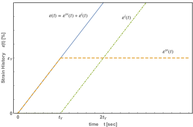
Figure 1: Imposed strain history $\varepsilon(t)$, viscoelastic $\varepsilon^{ve}(t)$ and inelastic $\varepsilon^{i}(t)$ deformation.

Taking into account the assumptions in Eq.s (6), (7) and (8), Figure 1 shows the imposed deformation history, the viscoelastic strain and the inelastic one. Usually, the limit value of the viscoelastic deformation $\varepsilon_{Y}$ is a function of the yield stress, $\varepsilon_{Y}=f(\sigma_{Y})$. Moreover, according to the Eq. (19) and under the aforementioned assumptions, the viscoelastic and inelastic deformation are

$$\varepsilon^{ve}(t)=\left\{\begin{split}&0,&&t<0,&\\ &\dot{\varepsilon}_{0}\,t,&&0\leqslant t<t_{Y},&\\ &\varepsilon_{Y},&&t\geqslant t_{Y},&\end{split}\right.$$ (20a)

$$\varepsilon^{i}(t)=\left\{\begin{split}&0,&&t<t_{Y},&\\ &\dot{\varepsilon}_{0}\,(t-t_{Y}),&&t\geqslant t_{Y}.&\\ \end{split}\right.$$ (20b)

For $$t\geqslant 0$$ strain histories in Eq.s (20b) may be rewritten as

$$\varepsilon^{ve}(t)=\dot{\varepsilon}_{0}\,t\,U(t_{Y}-t)+\varepsilon_{Y}\,U(t-t_{Y})$$ (21a)

$$\varepsilon^{i}(t)=\dot{\varepsilon}_{0}\,(t-t_{Y})\,U(t-t_{Y})$$ (21b)

3.1 Stress response for imposed strain history

By placing the strain histories of Eq.s (21b) into the fractional stress-strain relation of Eq. (13), the following relation holds true

$$\sigma(t)=\left\{\begin{split}&\bar{A}(\dot{\varepsilon}_{0})t^{1-\alpha},&&0<t<t_{Y},\\ &\bar{A}(\dot{\varepsilon}_{0})\left[t^{1-\alpha}-(t-t_{Y})^{1-\alpha}\right]+\bar{B}(\dot{\varepsilon}_{0})(t-t_{Y})^{1-\beta},&&t\geqslant t_{Y},\end{split}\right.$$ (22)

or in compact form

$$\sigma(t)=\bar{A}(\dot{\varepsilon}_{0})t^{1-\alpha}-\left[\bar{A}(\dot{\varepsilon}_{0})(t-t_{Y})^{1-\alpha}-\bar{B}(\dot{\varepsilon}_{0})(t-t_{Y})^{1-\beta}\right]U(t-t_{Y}),$$ (23)

where the involved coefficients are

$$\bar{A}(\dot{\varepsilon}_{0})=\frac{\tilde{A}\dot{\varepsilon}_{0}}{\Gamma(2-\alpha)},\;\;\;\;\;\;\;\bar{B}(\dot{\varepsilon}_{0})=\frac{\tilde{B}\dot{\varepsilon}_{0}}{\Gamma(2-\beta)}.$$ (24)

Moreover, taking into account the imposed strain history in Eq. (19) and performing a change of the variable from $t$ to $\varepsilon$, the relation in Eq. (23) can be rewritten as

$$\sigma(\varepsilon)=\bar{A}(\dot{\varepsilon}_{0})\varepsilon^{1-\alpha}-\left[\bar{A}(\dot{\varepsilon}_{0})(\varepsilon-\varepsilon_{Y})^{1-\alpha}-\bar{B}(\dot{\varepsilon}_{0})(\varepsilon-\varepsilon_{Y})^{1-\beta}\right]U(\varepsilon-\varepsilon_{Y}).$$ (25)

The five involved parameters $\tilde{A}$, $\alpha$, $\tilde{B}$, $\beta$ and $\varepsilon_{Y}$ have to be evaluated by performing a best-fitting of experimental data. Figure 2 shows some stress-strain relations obtained by Eq. (25) with different values of the involved parameters.

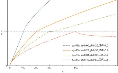
Figure 2: Stress-strain relation by Eq. (25) for different values of the parameters.

3.2 Idealized stress-strain curves from the proposed model

The proposed stress-strain relation in Eq. (25) represents a rate-dependent non-linear constitutive law describing the evolution of the stress during a displacement-control tensile tests. The model needs the definition of five parameters, that is, two coefficients $A$ and $B$ (anomalous moduli), two related fractional orders $\alpha$ and $\beta$, and a yielding value $\varepsilon_{Y}$.

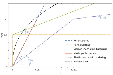
Figure 3: Some known cases obtained as particular case of the Eq. (25).

From the Eq. (25), with a proper selection of the involved five parameters, some the particular known cases reported in Figure 3 can be derived. In particular,

• if the yielding strain is such that $\varepsilon_{Y}\gg 0$, and the fractional order $\alpha=0$, then the anomalous modulus $A$ becomes the classical Young modulus $A=E$, and the perfect elastic case is obtained;

• if the yielding strain is such that $\varepsilon_{Y}\gg 0$, and the fractional order $\alpha=1$, then the anomalous modulus $A$ becomes the Newtonian viscosity $\mu$, and the proposed stress-strain relation leads to the perfect viscous model;

• if the yielding strain is such that $\varepsilon_{Y}=0$, $\alpha=1\Rightarrow A=\mu$, and $\beta=0\Rightarrow B=\tilde{E}$, a viscous linear strain hardening behavior is obtained;

• if the yielding strain is such that $\varepsilon_{Y}=\sigma_{Y}/A$, and $\alpha=0\Rightarrow A=E\gg B$, the elastic perfect plastic case is derived;

• if the yielding strain is such that $\varepsilon_{Y}=\sigma_{Y}/A$, $\alpha=0\Rightarrow A=E_{1}$, and $\beta=0\Rightarrow B=E_{2}$ another particular case is obtained, that is, the elastic linear strain hardening, where $E_{1}$ and $E_{2}$ are the stiffness before and after the yielding, respectively;

• if the yielding strain is zero, $\varepsilon_{Y}=0$, $\beta=n_{H}$, and $B=K\gg A$, according to Eq. (1), fractional stress-strain relation becomes the Hollomon law.

4 Best fitting of experimental data

The proposed stress-strain relation is used here to obtain a best-fitting of some experimental data. The considered experiments are reported in [16, 60, 61]. Such experiments regard a tensile test on two metals: AA60820-O aluminum alloy and AHSS TRIP 700 steel. Both tests are performed at room temperature with imposed strain ratio $\dot{\varepsilon}_{0}=0.001$ $s^{-1}$.

In order to show the capabilities of the proposed model, the best-fitting of experimental data obtained with the Eq. (25) is compared to the ones obtained with other known models. In particular, the classical models of Hollomon in Eq. (1) and Ramberg-Osgood in Eq. (2) are considered. Moreover, a recent rate-independent model based on fractional calculus, proposed by Mendiguren et al. in [16], is also considered. Such model is composed by two fractional terms and it needs the determination of four parameters. In particular, the stress-strain relation in [16] is obtained from the following fractional differential equation

$$a_{1}\left(D^{\alpha_{1}}\sigma\right)(\varepsilon)+a_{1}\left(D^{\alpha_{1}}\sigma\right)(\varepsilon)=1.$$ (26)

where the $\left(D^{\alpha_{j}}\sigma\right)(\varepsilon)$ denotes the $\alpha_{j}$-order Grunwald-Letinokov fractional derivative of the stress respect to the strain [54, 55, 56, 57, 58]. That is,

$$\left(D^{\alpha_{j}}\sigma\right)(\varepsilon)=\lim_{\Delta\varepsilon\to 0}\frac{1}{\Delta\varepsilon^{\alpha_{j}}}\sum_{k=0}^{\frac{t-\Delta\varepsilon}{\Delta\varepsilon}}\frac{\Gamma(k-\alpha_{j})}{\Gamma(-\alpha_{j})\Gamma(k-1)}\sigma(\varepsilon-j\Delta\varepsilon).$$ (27)

The solution of Eq. (28) is

$$\sigma(\varepsilon)=\sum_{k=0}^{\infty}\frac{(-1)^{k}a_{1}^{k}\,\varepsilon^{\alpha_{2}(k+1)-k\alpha_{1}}}{a_{2}^{k+1}\Gamma\left[\alpha_{2}(k+1)-k\alpha_{1}+1\right]},$$ (28)

where the parameters $a_{1}$, $\alpha_{1}$, $a_{2}$, and $\alpha_{2}$ for the considered experiments are detailed in [16].

The parameters resulting from the best fitting procedure of the proposed stress-strain relation in Eq. (25) and of the other three benchmark models are reported in Tables 1 and 2. In the first table the parameters of the AA60820-O aluminum alloy are reported, whereas the second one contains the parameters related to the AHSS TRIP 700 steel. The first three rods of the contain the parameters of the known models that are obtained in [42]. The five parameters of the proposed model are reported in the forth rods, they are obtained by least-squares method with the aid of the software Wolfram Mathematica.

Model	Parameters
Hollomon Eq. (1)	$K$ (MPa)	$n_{H}$
	$235.77$	$0.1812$
Ramberg-Osgood Eq. (2)	$E$ (MPa)	$n_{RO}$	$H$ (MPa)
	$70000.00$	$5.7452$	$233.07$
Mendiguren et al. Eq. (28)	$a_{1}$ (MPa-1)	$\alpha_{1}$	$a_{2}$ (MPa-1)	$\alpha_{2}$
	$4.6411\times 10^{-3}$	$0.1710$	$1.4286\times 10^{-5}$	$1.0000$
Fractional stress-strain relation Eq. (25)	$\bar{A}$ (MPa)	$\alpha$	$\bar{B}$ (MPa)	$\beta$	$\varepsilon_{Y}$
	$24516.6108$	$0.1500$	$233.72$	$0.7191$	$0.0011$

Table 1: Parameters of AA60820-O aluminum alloy.

Model	Parameters
Hollomon Eq. (1)	$K$ (MPa)	$n_{H}$
	$1253.90$	$0.2202$
Ramberg-Osgood Eq. (2)	$E$ (MPa)	$n_{RO}$	$H$ (MPa)
	$203000.00$	$4.8267$	$1230.10$
Mendiguren et al. Eq. (28)	$a_{1}$ (MPa-1)	$\alpha_{1}$	$a_{2}$ (MPa-1)	$\alpha_{2}$
	$8.8637\times 10^{-4}$	$0.2034$	$4.92611\times 10^{-6}$	$0.0012$
Fractional stress-strain relation Eq. (25)	$\bar{A}$ (MPa)	$\alpha$	$\bar{B}$ (MPa)	$\beta$	$\varepsilon_{Y}$
	$70000.00$	$0.1820$	$1271.83$	$0.6365$	$0.0023$

Table 2: Parameters of AHSS TRIP 700 steel.

Figure 4 shows the stress-strain relation during the whole tensile test for both the materials. Figure 4(a) shows the experimental data (dotted line) of the AA60820-O aluminum alloy, the fitting laws of the proposed model and of other three, using the parameters reported in Table 1. Figure 4(b) shows the comparison between experimental data of AHSS TRIP 700 steel, the proposed model and the others, for which the parameters are reported in Table 2. From these figures it is possible to observe that the best agreements with the considered experimental data are obtained with the proposed fractional stress-strain relation.

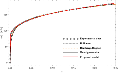
(a) AA60820-O Aluminum Alloy

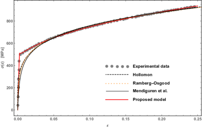
(b) AHSS TRIP 700 Steel

Figure 4: Stress-strain relation: experimental data and four fitted models.

Figures 5 show the details of the stress-strain curves close the yielding point. From these figures it can be observed that the proposed model is able to fit experimental data with excellent accuracy in this particular zone of the curves. Moreover, the proposed model is also able to fit the experimental results also for large strain. In particular, in Figure 6 the comparisons between the experimental data and the considered models for large value of strain are reported. Observe that also in this case the proposed model guarantees the best agreement between theoretical and experimental results.

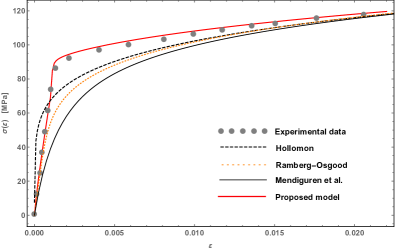
(a) AA60820-O Aluminum Alloy

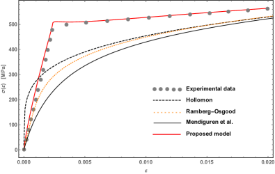
(b) AHSS TRIP 700 Steel

Figure 5: Enlargement of the stress-strain relation near the yielding point: experimental data and four fitted models.

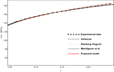
(a) AA60820-O Aluminum Alloy

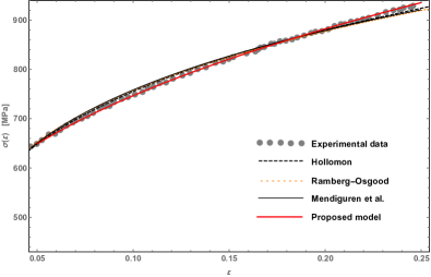
(b) AHSS TRIP 700 Steel

Figure 6: Enlargement of the stress-strain relation for large strain: experimental data and four fitted models.

As can be seen from the Figures 4 and 6, all the models offer a good agreement for greater value of the deformation, but Figures 5 show that only the proposed model is also able to simulate the initial stress-strain relation with a good agreement with the experimental tests.

For the comparison between the different laws and the evaluation of the accuracy of the models for the best-fitting, two error parameters are evaluated: the mean square error ($MSE$) and the mean absolute percentage error ($MAPE$). $MSE$ measures the average of the squares of the errors. It is defined as the difference between the exact value and theoretical one obtained by the model. That is,

$$MSE=\frac{1}{n}\sum_{j=1}^{n}\left[\sigma_{j}-\sigma(\varepsilon_{j})\right]^{2},$$ (29)

where $\sigma_{j}$ is $i$-th experimental value of the stress, and $\sigma(\varepsilon_{j})$ is the stress obtained by the considered model for the $i$-the experimental stress, $n$ are the considered experimental values. The other error parameter, $MAPE$, provides an evaluation of the quality of the considered models in the estimation. It usually expresses accuracy as a percentage by the following expression

$$MAPE=\frac{100\,\%}{n}\sum_{j=1}^{n}\left|\frac{\sigma_{j}-\sigma(\varepsilon_{j})}{\sigma_{j}}\right|.$$ (30)

Both parameters are reported for all the considered models in Table 3 and 4. In particular, in Table 3 the $MSEs$ and $MAPEs$ related to the experimental data of the AA60820-O aluminum alloy are reported, while Table 4 shows the error parameters of best fitting procedure for the AHSS TRIP 700 steel data.

Model	$\boldsymbol{MSE}$	$\boldsymbol{MAPE}$
Hollomon Eq. (1)	$46.7713$	$8.89\,\%$
Ramberg-Osgood Eq. (2)	$45.1300$	$5.34\,\%$
Mendiguren et al. Eq. (28)	$112.6147$	$7.98\,\%$
Fractional stress-strain relation Eq. (25)	$4.5657$	$2.61\,\%$

Table 3: MSEs and MREs of AA60820-O aluminum alloy data best-fitting.

Model	$\boldsymbol{MSE}$	$\boldsymbol{MAPE}$
Hollomon Eq. (1)	$1061.7008$	$4.47\,\%$
Ramberg-Osgood Eq. (2)	$1165.0348$	$3.37\,\%$
Mendiguren et al. Eq. (28)	$997.2121$	$5.01\,\%$
Fractional stress-strain relation Eq. (25)	$160.1546$	$1.84\,\%$

Table 4: MSEs and MREs of AHSS TRIP 700 steel data best-fitting.

From such tables, it is possible to observe that the lowest value of the error is obtained by the stress-strain relation in Eq. (25). Therefore, the best agreement with the experimental data is obtained by the proposed mechanical model.

The proposed stress-strain relation is able to fit the mechanical behavior before and after the yielding point. Compared to the other models, the proposed model is able to better describe the mechanical behavior near the yielding point. Such major capability to fit experimental data is related to three fundamental aspects of the proposed model. In particular, i) viscoelastic stress-strain relation is represented by Boltzmann superposition integral with power-law kernel; ii) the yielding phenomenon activates an inelastic behavior; iii) the inelastic stress-strain relation is modeled by an integral formulation with non-linear kernel.

The proposed stress-strain relation is non-linear after the yielding phenomenon, however for particular cases it becomes just the summation of two fractional derivatives with different orders. The appearance of these two linear operators simplified the stress-strain relation. Therefore, although the model requires the evaluation of five parameters, for the considered cases, the evaluation of the mechanical parameters is easy.

5 Concluding remarks

Considering the evidence presented above, it is evident that the proposed stress-strain relation is able to predict accurately the mechanical behavior of metals during the tensile test. Such stress-strain relation may take into account both viscoelastic and plastic behaviors. It has been obtained as an integral formulation of the constitutive law. The model is similar to the endochronic theory of plasticity introduced by Valanis. The main difference between the proposed model and the Valanis’ theory lies in two aspects, that is, the definition of the yielding surface and the use of a time power-law kernel in the convolution integrals.

The proposed model provides a non-linear formulation of the stress-strain relation. However, if the strain history is a monotonic increasing function of time, the stress history becomes a summation of two time fractional derivatives of the strain history. The first one describes the viscoelastic stress, while the second one is related to the mechanical behavior after the yielding phenomenon.

Considering that the most used test for the characterization of the mechanical properties of the materials is the tensile one, the stress-strain relation has been particularized for the case in which the imposed strain history is a ramp function in time. It is shown that, for the tensile test, the stress-strain relation becomes a summation of power-law functions with five parameters. Such parameters have been evaluated by a best-fitting procedure for two metal alloys. After the parameter evaluation, the results of the proposed model have been compared to other ones obtained from other known models. Such comparison has shown that the proposed model offers the best agreement with the experimental data and the lowest level of the error.

References

- [1] Franchi R, Del Prete A, Donatiello I, Calabrese M. Ring rolling process simulation for geometry optimization. AIP Conference Proceedings 2017; 1896:190010.
- [2] Outeiro JC, Umbrello D, MŚaoubi R, Jawahir I. Evaluation of numerical models for predicting surface integrity in metal machining. Machining Science and Technology 2015; 19(2):183-216.
- [3] Del Prete A, Filice L, Umbrello D. Numerical simulation of machining nickel-based alloys. Procedia CIRP 2013; 8:540-545.
- [4] Franchi R, Del Prete A, Umbrello D. Inverse analysis procedure to determine flow stress and friction data for finite element modeling of machining. International Journal of Material Forming 2017; 10(5):685-695.
- [5] Mendelson A. Plasticity: Theory and Applications. Macmillan Publishing; 1968.
- [6] Malvern L E. Introduction to the Mechanics of a Continuous Mechanis. Prentice-Hall, Inc.; 1969.
- [7] Lubliner J. Plasticity Theory. Macmillan Publishing; 1990.
- [8] Simo JC, Hughes TJ. Computational Inelasticity. Springer; 1994.
- [9] Han-Chin W. Continuum Mechanics and Plasticity. Chapman & Hall/Crc; 2005
- [10] Hollomon JH. Tensile deformation. Transactions of the Metallurgical Society of AIME 1945;162:268-90.
- [11] Holmquist JL, and Nàdai A. A theoretical and experimental approach to the problem of collapse of deep-well casing. Paper presented at 20th Annual Meeting, Am. Petroleum Inst., Chicago, Nov. 1939.
- [12] Ramberg W, Osgood WR. Description of stress-strain curves by three Parameters, Technical note no 902. Washington, DC: National Advisory Committee for Aeronautics; 1943.
- [13] Bao G, Hutchinson JW, McMeeking RM.Particle reinforcement of ductile matrices against plastic flow and creep. Acta Metallurgica et Materialia 1991; 39(8):1871-1882.
- [14] Tiryakioglu M, Staley JT, Campbell J. Comparative study of the constitutive equations to predict the work hardening characteristics of cast Al-7wt.%Si-0.20wt.%Mg alloys Journal of Materials Science Letters 2000; 19(24):2179-2181.
- [15] Yetna N’Jock M, Chicot D, Decoopman X, Lesage J, Ndjaka JM, Pertuz A. Mechanical tensile properties by spherical macroindentation using an indentation strain-hardening exponent International Journal of Mechanical Sciences 2013; 75:257-264.
- [16] Mendiguren J, Cortés F, Galdos L. A generalised fractional derivative model to represent elastoplastic behaviour of metals. International Journal of Mechanical Sciences 2012; 65(1):12-17.
- [17] Rees DWA. Plane strain compression of aluminium alloy sheets. Materials & Design 2012; 39:495-503.
- [18] Baldi A, Medda A, Bertolino F. Comparing two different approaches to the identification of the plastic parameters of metals in post-necking regime. Experimental and Applied Mechanics 2011; 6:727-732.
- [19] Ludwigson DC. Modified stress-strain relation for FCC metals and alloys. Metallurgical Transanctions 1971; 2:2825-8.
- [20] Swift HW. Plastic instability under plane stress. Journal of the Mechanics and Physics of Solids 1952; 1:1-18.
- [21] Ludwick P. Element der technologischen mechanik. Berlin: Springer-Verlag; 32-37.
- [22] Caddemi S. Parametric nature of the non-linear hardening plastic constitutive equations and their integration. European Journal of Mechanics - A/Solids 1998; 17(3):479-498.
- [23] Cernocky EP, Krempl E. A non-linear uniaxial integral constitutive equation incorporating rate effects, creep and relaxation. International Journal of Non-Linear Mechanics 1979; 14(3):183-203.
- [24] Auricchio F. A viscoplastic constitutive equation bounded between two generalized plasticity. International Journal of Plasticity 1997; 13(8-9):697-721.
- [25] Auricchio F, Taylor RL. A generalized visco-plasticity model and its algorithmic implementation. Computers & Structures 1994; 53(3):637-647.
- [26] Deseri L, Mares R. A class of viscoelastoplastic constitutive models based on the maximum dissipation principle. Mechanics of Materials 200; 32:389-403
- [27] Flügge W. Viscoelasticity. Berlin: Springer-Verlag; 1976.
- [28] Christensen RM. Theory of Viscoelasticity. Dover Publications, Inc., New York; 2003.
- [29] Valanis KC. A theory of viscoplasticity without a yield surface, Arch. Mech. 1971; 23, 517, 1971.
- [30] Valanis, KC, Read HE. A theory of plasticity for hysteretic materials-I: Shear response. Computers and Structures 1978; 8(3-4):503-510.
- [31] Valanis KC. Fundamental consequences of a new intrinsic time measure plasticity as a limit of the endochronic theory. Arch. Mech. 1980; 32, 171.
- [32] Valanis KC, Lee C-F. Some recent developments of the endochronic theory with applications. Nuclear Engineering and Design 1982; 69(3):327-344.
- [33] Valanis KC, Fan J. Endochronic analysis of cyclic elastoplastic strain fields in a notched plate. American Society of Mechanical Engineers 1983; 50:789-794.
- [34] Bazant ZP. Endochronic inelasticity and incremental plasticity. International Journal of Solids and Structures 1978; 14(9):691-714.
- [35] Peng X, Ponter ARS. Extremal properties of endochronic plasticity, part I: Extremal path of the constitutive equation without a yield surface. International Journal of Plasticity 1993; 9(5):551-566.
- [36] Koeller RC. Applications of fractional calculus to theory of viscoelasticity. Journal of Applied Mechanics 1984; 51:299-307.
- [37] Makris N. Three-dimensional constitutive viscoelastic laws with fractional order time derivatives. Journal of Rheology 1997; 41(5):1007-1020.
- [38] Alotta G, Barrera O, Cocks ACF, Di Paola M. On the behavior of a three-dimensional fractional viscoelastic constitutive model. Meccanica 2017; 52(9):2127-2142.
- [39] Yu HY. Variation of elastic modulus during plastic deformation and its influence on springback. Materials and Design 2009; 30(3):846-850.
- [40] Thibaud S, Boudeau N, Gelin JC. Influence of initial and induced hardening in sheet metal forming. Int. J. Damage Mech 2002; 13:107-122.
- [41] Halilovič M, Vrh M, Štok B. Impact of elastic modulus degradation on spring-back in sheet metal forming. AIP conference proceedings 2008; 908(1):925-930.
- [42] Mendiguren J, Trujillo JJ, Cortés F, Galdos L. An extended elastic law to represent non-linear elastic behaviour: Application in computational metal forming. International Journal of Mechanical Science 2013; 77:57-64.
- [43] Di Mino G, Airey G, Di Paola M, Pinnola FP, D’Angelo G, Lo Presti D. Linear and nonlinear fractional hereditary constitutive laws of asphalt mixtures. Journal of Civil Engineering and Management 2016; 22(7):882-889.
- [44] Meng R, Yin D, Zhou C, Wu H. Fractional description of time-dependent mechanical property evolution in materials with strain softening behavior. Applied Mathematical Modelling 2016; 40:398-406.
- [45] Nutting PG. A new general law of deformation. Journal of the Franklin Institute 1921; 191:679-685.
- [46] Gemant A. A method of analyzing experimental results obtained by elasto-viscous bodies. Journal of Physics 1936; 7:311-17.
- [47] Nutting PG. A general stress-strain-time formula. Journal of the Franklin Institute 1943; 225:513-524.
- [48] Di Paola M, Pirrotta A, Valenza A. Visco-elastic behavior through fractional calculus: An easier method for best fitting experimental results. Mechanics of Materials 2011; 43:799-806.
- [49] Di Paola M, Fiore V, Pinnola FP, Valenza A. On the influence of the initial ramp for a correct definition of the parameters of fractional viscoelastic materials. Mechanics of Materials 2014; 69:63-70.
- [50] Alotta G, Di Paola M, Pirrotta A. Fractional Tajimi-Kanai model for simulating earthquake ground motion. Bullettin of Earthquake Engineering 2014, 12:2495-2506.
- [51] Zhu S, Cai C, Spanos PD. A nonlinear and fractional derivative viscoelastic model for rail pads in the dynamic analysis of coupled vehicle-slab track systems. Journal of Sound and Vibration 2015; 335:304-320.
- [52] Alotta G, Colinas-Armijo N. Analysis of fractional viscoelastic material with mechanical parameters dependent on random temperature. ASCE-ASME Journal of Risk and Uncertainty in Engineering Systems, Part B: Mechanical Engineering 2017; 3(3):030906.
- [53] Du M, Wang Y, Wang Z. Effect of the initial ramps of creep and relaxation tests on models with fractional derivatives. Meccanica 2017; 52(15):3541-3547.
- [54] Oldham KB, Spainer J. The Fractional Calculus: Theory and applications of differentiation and integration to arbitrary order, Academic Press, New York, 1974.
- [55] Samko GS, Kilbas AA, Marichev OI. Fractional integrals and derivatives: theory and applications, New York (NY): Gordon and Breach, 1993.
- [56] Miller KS, Ross B. An Introduction to the Fractional Calculus and Fractional Differential Equations, Wiley-InterScience, New York, 1993.
- [57] Podlubny I. Fractional Differential Equations, Academic Press, San Diego, 1999.
- [58] Kilbas AA, Srivastava HM, Trujillo JJ. Theory and Applications of Fractional Differential Equations, Elsevier, Amsterdam, 2006.
- [59] Yin D, Zhang W, Cheng C, Yi L. Fractional time-dependent Bingham model for muddy clay, Journal of Non-Newtonian Fluid Mechanics 2012; 187-188:32-35.
- [60] Aginagalde A, Gómez X, Galdos L, García C. Heat treatment selection and forming strategies for 6082 aluminum alloy, Journal of Engineering Materials and Technology 2009; 131:044501.
- [61] Perez R, Benito J, Prado J. Study of the inelastic response of TRIP steels after plastic deformation, ISIJ International 2005; 45(12):1925-33.