A Logic Based Approach to Finding Real Singularities of Implicit Ordinary Differential Equations

Abstract

We discuss the effective computation of geometric singularities of implicit ordinary differential equations over the real numbers using methods from logic. Via the Vessiot theory of differential equations, geometric singularities can be characterised as points where the behaviour of a certain linear system of equations changes. These points can be discovered using a specifically adapted parametric generalisation of Gaussian elimination combined with heuristic simplification techniques and real quantifier elimination methods. We demonstrate the relevance and applicability of our approach with computational experiments using a prototypical implementation in Reduce.

1. Introduction

Implicit differential equations, i. e. equations which are not solved for a derivative of highest order, appear in many applications. In particular, the so-called differential algebraic equations (DAE) may be considered as a special case of implicit equations. Compared with equations in solved form, implicit equations are more complicated to analyse and show a much wider range of phenomena. Already basic questions about the existence and uniqueness of solutions of an initial value problem become much more involved. One reason is the possible appearance of singularities. Note that we study in this work singularities of the differential equations themselves (defined below in a geometric sense) and not singularities of individual solutions like poles.

Our approach to singularities of differential equations is conceptually based on the theory of singularities of maps between smooth manifolds (as e. g. described in [2, 22]), i. e. of a differential topological nature. Within this theory, the main emphasis has traditionally been on classifying possible types of singularities and on corresponding normal forms, see e. g. [13, 14]. Nice introductions can be found in [1] or [36]. By contrast, we are here concerned with the effective detection of all geometric singularities of a given implicit ordinary differential equation. This requires the additional use of techniques from differential algebra [30, 38] and algebraic geometry [12].

In [33], the first two authors developed together with collaborators a novel framework for the analysis of algebraic differential equations, i. e. differential equations (and inequations) described by differential polynomials, which combines ideas and techniques from differential algebra, differential geometry and algebraic geometry. A key role in this new effective approach is played by the Thomas decomposition which exists in an algebraic version for algebraic systems and in a differential version for differential systems. Both were first introduced by Thomas [51, 52] and later rediscovered by Gerdt [20]; an implementation in Maple is described in [4] (see also [21]). Unfortunately, the algorithms behind the Thomas decomposition require that the underlying field is algebraically closed. Hence, it is always assumed in [33] that a complex differential equation is treated. However, most differential equations appearing in applications are real. The main goal of this work is to adapt the framework of [33] to real ordinary differential equations.

The approach in [33] consists of a differential and an algebraic step. For the prepatory differential step, one may continue to use basic differential algebraic algorithms (for example the differential Thomas decomposition). A key task of the differential step is to exhibit all integrability conditions which may be hidden in the given system and for this the base field does not matter. In this work, we are mainly concerned with presenting an alternative for the algebraic step – where the actual identification of the singularities happens – which is valid over the real numbers.

Our use of real algebraic geometry combined with computational logic has several benefits. In a complex setting, one may only consider inequations. Over the reals, also the treatment of inequalities like positivity conditions is possible which is important for many applications e. g. in biology and chemistry. We will extend the approach from [33] by generalising the notion of an algebraic differential equation used in [33] to semialgebraic differential equations, which allow for arbitrary inequalities. As a further improvement, we will make stronger use of the fact that the detection of singularities represents essentially a linear problem. This will allow us to avoid some redundant case distinctions that are unavoidable in the approach of [33], as they must appear in any algebraic Thomas decomposition, although they are irrelevant for the detection of singularities.

The article is structured as follows. The next section firstly exhibits some basics of the geometric theory of (ordinary) differential equations. We then recapitulate the key ideas behind the differential step of [33] and encapsulate the key features of the outcome in the improvised notion of a “well-prepared” system. Finally, we define the geometric singularities that are studied here. In the third section, we develop a Gauss algorithm for linear systems depending on parameters with certain extra features and rigorously prove its correctness. The fourth section represents the core of our work. We show how finding geometric singularities can essentially be reduced to the analysis of a parametric linear system and present then an algorithm for the automatic detection of all real geometric singularities based on our parametric Gauss algorithm. The fifth section demonstrates the relevance of our algorithm by applying it to some basic examples some of which stem from the above mentioned classifications of all possible singularities of scalar first-order equations. Although these examples are fairly small, it becomes evident how our logic based approach avoids some unnecessary case distinctions made by the algebraic Thomas decomposition.

2. Geometric Singularities of Implicit Ordinary Differential Equations

We use the basic set-up of the geometric theory of differential equations following [41] to which we refer for more details. For a system of ordinary differential equations of order $\ell$ in $m$ unknown real-valued functions $u_{\alpha}(t)$ of the independent real variable $t$, we construct over the trivial fibration $\pi=\mathrm{pr}_{1}:\mathbbm{R}\times\mathbbm{R}^{m}\rightarrow\mathbbm{R}$ the $\ell$th order jet bundle $J_{\ell}\pi$. For our purposes, it is sufficient to imagine $J_{\ell}\pi$ as an affine space diffeomorphic to $\mathbbm{R}^{(\ell+1)m+1}$ with coordinates $(t,\mathbf{u},\mathbf{\dot{u}}\dots,\mathbf{u}^{(\ell)})$ corresponding to the independent variable $t$, the $m$ dependent variables $\mathbf{u}=(u_{1},\dots,u_{m})$ and the derivatives of the latter ones up to order $\ell$. We denote by $\pi^{\ell}:J_{\ell}\pi\rightarrow\mathbbm{R}$ the canonical projection on the first coordinate. The contact structure is a geometric way to encode the different roles played by the different variables, i. e. that $t$ is the independent variable and that $u_{\alpha}^{(i)}$ denotes the derivative of $u_{\alpha}^{(i-1)}$ with respect to $t$. We describe the contact structure by the contact distribution $\mathcal{C}^{(\ell)}\subset TJ_{\ell}\pi$ which is spanned by one $\pi^{\ell}$-transversal and $m$ $\pi^{\ell}$-vertical vector fields:

$$C^{(\ell)}_{\mathrm{trans}}=\partial_{t}+\sum_{i=1}^{\ell}\sum_{\alpha=1}^{m}u_{\alpha}^{(i)}\cdot\partial_{u_{\alpha}^{(i-1)}}\,,\qquad C^{(\ell)}_{\alpha}=\partial_{u_{\alpha}^{(\ell)}}\quad(\alpha=1,\dots,m)\,.$$

The transversal field essentially corresponds to a geometric version of the chain rule and the vertical fields are needed because we must cut off the chain rule at a finite order, since in $J_{\ell}\pi$ no variables exist corresponding to derivatives of order $\ell+1$ required for the next terms in the chain rule.

We can now rigorously define the class of differential equations that will be studied in this work. Note that in the geometric theory one does not distinguish between a scalar equation and a system of equations, as a differential equation is considered as a single geometric object independent of its codimension. In [33], an algebraic jet set of order $\ell$ is defined as a locally Zariski closed subset of $J_{\ell}\pi$, i. e. as the set theoretic difference of two varieties. This approach reflects the fact that over the complex numbers only equations and inequations are allowed. Over the real numbers, one would like to include arbitrary inequalities like for example positivity conditions. Thus it is natural to proceed from algebraic to semialgebraic geometry. Recall that a semialgebraic subset of $\mathbbm{R}^{n}$ is the solution set of a Boolean combination of conditions of the form $f=0$ or $f\diamond 0$ where $f$ is a polynomial in $n$ variables and $\diamond$ stands for some relation in $\{<,>,\leq,\geq,\neq\}$ (see e. g. [8, Chap. 2]).

Definition 1.

A semialgebraic jet set of order $\ell$ is a semialgebraic subset $\mathcal{J}_{\ell}\subseteq J_{\ell}\pi$ of the $\ell$th order jet bundle. Such a set is a semialgebraic differential equation, if in addition the Euclidean closure of $\pi^{\ell}(\mathcal{J}_{\ell})$ is the whole base space $\mathbbm{R}$.

In the traditional geometric theory, a differential equation is a fibred submanifold of $J_{\ell}\pi$ such that the restriction of $\pi^{\ell}$ to it defines a surjective submersion. The latter condition excludes any kind of singularities and is thus dropped in our approach. We replace the submanifold by a semialgebraic and thus in particular constructible set, i. e. a finite union of locally Zariski closed sets. This is on the one hand more restrictive, as only polynomial equations and inequalities are allowed. On the other hand, it is more general, as a semialgebraic set may have singularities in the sense of algebraic geometry. We will call such points algebraic singularities of the semialgebraic differential equation $\mathcal{J}_{\ell}$ to distinguish them from the geometric singularities on which we focus in this work.

The additional closure condition imposed in Definition 1 for a semialgebraic differential equation ensures that the semialgebraic differential system defining it does not contain equations depending solely on $t$ and thus that $t$ represents indeed an independent variable. Nevertheless, we admit that certain values of $t$ are not contained in the image $\pi^{\ell}(\mathcal{J}_{\ell})$. This relaxation compared with the standard geometric theory allows us to handle equations like $t\dot{u}=1$ where the point $t=0$ is not contained in the projection. We use the Euclidean closure instead of the Zariski one, as for a closer analysis of the solution behaviour around such a point (which we will not do in this work) it is of interest to consider the point as the limit of a sequence of points in $\pi^{\ell}(\mathcal{J}_{\ell})$.

A (sufficiently often differentiable) function $\mathbf{g}:\mathcal{I}\subseteq\mathbbm{R}\rightarrow\mathbbm{R}^{m}$ defined on some interval $\mathcal{I}$ is a (local) solution of the semialgebraic differential equation $\mathcal{J}_{\ell}\subset J_{\ell}\pi$, if its prolonged graph, i. e. the image of the curve $\gamma_{\mathbf{g}}:\mathcal{I}\rightarrow J_{\ell}\pi$ given by $t\mapsto\bigl{(}t,\mathbf{g}(t),\mathbf{\dot{g}}(t),\dots,\mathbf{g}^{(\ell)}(t)\bigr{)}$ lies completely in the set $\mathcal{J}_{\ell}$. This definition of a solution represents simply a geometric version of the usual one. Figure 1 shows the semialgebraic differential equation $\mathcal{J}_{1}$ which is defined by the scalar first-order equation $\dot{u}-tu^{2}=0$ together with some of its prolonged solutions. $\mathcal{J}_{1}$ is a classical example of a differential equation with so-called movable singularities: its solutions are given by $u(t)=2/(c-t^{2})$ with an arbitrary constant $c\in\mathbbm{R}$ and each solution with a positive $c$ becomes singular after a finite time. However, this differential equation does not exhibit the kind of singularities that we will be studying in this work. We are concerned with singularities of the differential equation itself and not with singularities of individual solutions.

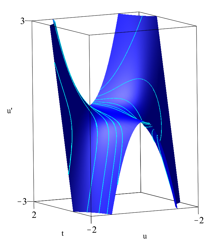
Figure 1. A semialgebraic differential equation with some prolonged solutions

We call a semialgebraic jet set $\mathcal{J}_{\ell}\subseteq J_{\ell}\pi$ basic, if it can be described by a finite set of equations $p_{i}=0$ and a finite set of inequalities $q_{j}>0$ where $p_{i}$ and $q_{j}$ are polynomials in the coordinates $(t,\mathbf{u},\mathbf{\dot{u}}\dots,\mathbf{u}^{(\ell)})$. We call such a pair of sets a basic semialgebraic system on $J_{\ell}\pi$. It follows from an elementary result in real algebraic geometry [8, Prop. 2.1.8] that any semialgebraic jet set can be expressed as a union of finitely many basic semialgebraic jet sets. We will always assume that our sets are given in this form and study each basic semialgebraic system separately, as for some steps in our analysis it is crucial that at least the equation part of the system is a pure conjunction.

To obtain correct and meaningful results with our approach, we need some further assumptions on the basic semialgebraic differential systems we are studying. More precisely, the systems have to be carefully prepared using a procedure essentially corresponding to the differential step of the approach developed in [33] and the subsequent transformation from a differential algebraic formulation to a geometric one. Otherwise, hidden integrability conditions or other subtle problems may lead to false results. We present here only a very brief description of this procedure and refer for all details and an extensive discussion of the underlying problems to [33]. We use in the sequel some basic notions from differential algebra [30, 38] and the Janet–Riquier theory of differential equations [27, 37] which can be found in modern form for example in [39] to which we refer for definitions of all unexplained terminology and for background information.

The starting point of our analysis will always be a basic semialgebraic system with equations $p_{i}=0$ $(1\leq i\leq r)$ and inequalities $q_{j}>0$ $(1\leq j\leq s)$. We call such a system differentially simple with respect to some orderly ranking $\prec$, if it satisfies the following three conditions:

1. all polynomials $p_{i}$ and $q_{j}$ are non-constant and have pairwise different leaders,

2. no leader of an inequality $q_{j}$ is a derivative of the leader of an equation $p_{i}$,

3. away from the variety defined by the vanishing of all the initials and all the separants of the polynomials $p_{i}$, the equations define a passive differential system for the Janet division.

The last condition ensures the absence of hidden integrability conditions and thus the existence of formal solutions (i. e. solutions in the form of power series without regarding their convergence) for almost all initial conditions. In the sequel, we will always assume that in addition our system is not underdetermined, i. e. that its formal solution space is finite-dimensional. Differentially simple systems can be obtained with the differential Thomas decomposition.

Consider the ring of differential polynomials $\mathcal{D}=\mathbbm{R}(t)\{\mathbf{u}\}$. Obviously, the polynomials $p_{i}$ may be considered as elements of $\mathcal{D}$ and we denote by $\hat{\mathcal{I}}=\langle p_{1},\dots,p_{r}\rangle_{\mathcal{D}}$ the differential ideal generated by the equations in our differentially simple system. It turns out that in some respect this ideal is too small and therefore we saturate it with respect to the differential polynomial $Q=\prod_{i=1}^{r}\mathrm{init}(p_{i})\mathrm{sep}(p_{i})$ to obtain the differential ideal $\mathcal{I}=\hat{\mathcal{I}}:Q^{\infty}$ of which one can show that it is the radical of $\hat{\mathcal{I}}$ [39, Prop. 2.2.72]. Over the real numbers, we need the potentially larger real radical according to the real nullstellensatz (see e. g. [8, Sect. 4.1] for a discussion). An algorithm for determining the real radical was proposed by Becker and Neuhaus [7, 34]. An implementation over the rational numbers exists in Singular [44]. However, in all these references it is assumed that one deals with an ideal in a polynomial ring with finitely many variables. Thus we have to postpone the determination of the real radical until we have obtained such an ideal.

For the transition from differential algebra to jet geometry, we introduce for any finite order $\ell\in\mathbbm{N}$ the finite-dimensional subrings $\mathcal{D}_{\ell}=\mathcal{D}\cap\mathbbm{R}[t,\mathbf{u},\dots,\mathbf{u}^{(\ell)}]$. Note that $\mathcal{D}_{\ell}$ is the coordinate ring of the jet bundle $J_{\ell}\pi$ considered as an affine space. Fixing some order $\ell\in\mathbbm{N}$ which is at least the maximal order of an equation $p_{i}=0$ or an inequality $q_{j}>0$, we define the polynomial ideal $\hat{\mathcal{I}}_{\ell}=\hat{\mathcal{I}}\cap\mathcal{D}_{\ell}$. Using Janet–Riquier theory and Gröbner basis techniques, it is straightforward to construct an explicit generating set of this ideal. Now that we have an ideal in a polynomial ring with finitely many variables, we can determine its real radical $\mathcal{I}_{\ell}$. Finally, we prefer to work with irreducible sets and thus perform a real prime decomposition of the ideal $\mathcal{I}_{\ell}$ and study each prime component separately. Thus we may assume in the sequel without loss of generality that the given polynomials $p_{i}$ generate directly a real prime ideal $\mathcal{I}_{\ell}\subset\mathcal{D}_{\ell}$.

Definition 2.

A basic semialgebraic differential equation $\mathcal{J}_{\ell}\subset J_{\ell}\pi$ is called well prepared, if it is obtained by the above outlined procedure starting from a differentially simple system.

Consider a (local) solution $\mathbf{g}:\mathcal{I}\subseteq\mathbbm{R}\rightarrow\mathbbm{R}^{m}$ of a semialgebraic differential equation $\mathcal{J}_{\ell}$ and the corresponding curve $\gamma_{\mathbf{g}}:\mathcal{I}\rightarrow J_{\ell}\pi$ given by $t\mapsto\bigl{(}t,\mathbf{g}(t),\mathbf{\dot{g}}(t),\dots,\mathbf{g}^{(\ell)}(t)\bigr{)}$. Since, according to our definition of a solution, $\mathrm{im}\,\gamma_{\mathbf{g}}\subseteq\mathcal{J}_{\ell}$, for each $t\in\mathcal{I}$ the tangent vector $\gamma_{\mathbf{g}}^{\prime}(t)$ must lie in the tangent space $T_{\gamma_{\mathbf{g}}(t)}\mathcal{J}_{\ell}$ of $\mathcal{J}_{\ell}$ at the point $\gamma_{\mathbf{g}}(t)\in\mathcal{J}_{\ell}$. We mentioned already above the contact structure of the jet bundle. It characterises intrinsically those (transversal) curves $\gamma:\mathcal{I}\subseteq\mathbbm{R}\rightarrow J_{\ell}\pi$ that are prolonged graphs. More precisely, there exists a function $\mathbf{g}:\mathcal{I}\rightarrow\mathbbm{R}^{m}$ such that $\gamma=\gamma_{\mathbf{g}}$, if and only if the tangent vector $\gamma^{\prime}(t)$ is contained in the contact distribution $\mathcal{C}^{(\ell)}|_{\gamma(t)}$ evaluated at $\gamma(t)$. These two observations motivate the following definition of the space of all “infinitesimal solutions” of the differential equation $\mathcal{J}_{\ell}$.

Definition 3.

Given a point $\rho$ on a semialgebraic jet set $\mathcal{J}_{\ell}\subseteq J_{\ell}\pi$, we define the Vessiot space at $\rho$ as the linear space $\mathcal{V}_{\rho}[\mathcal{J}_{\ell}]=T_{\rho}\mathcal{J}_{\ell}\cap\mathcal{C}^{(\ell)}|_{\rho}$.

In general, the properties of the Vessiot spaces $\mathcal{V}_{\rho}[\mathcal{J}_{\ell}]$ depend on their base point $\rho$. In particular, at different points the Vessiot spaces may have different dimensions. Nevertheless, it is easy to show that for a well-prepared semialgebraic differential equation $\mathcal{J}_{\ell}$ the Vessiot spaces define a smooth regular distribution on a Zariski open and dense subset of $\mathcal{J}_{\ell}$ (see e. g. [33, Prop. 2.10] for a rigorous proof). Therefore, with only a minor abuse of language, we will call the family of all Vessiot spaces the Vessiot distribution $\mathcal{V}[\mathcal{J}_{\ell}]$ of the given differential equation $\mathcal{J}_{\ell}$.

We will ignore here algebraic singularities of a semialgebraic differential equation $\mathcal{J}_{\ell}$, i. e. points on $\mathcal{J}_{\ell}$ that are singularities in the sense of algebraic geometry. It is a classical task in algebraic geometry to find them, e. g. with the Jacobian criterion which reduces the problem to linear algebra [12, Thm. 9.6.9]. We will focus instead on geometric singularities. In the here exclusively considered case of not underdetermined ordinary differential equations, we can use the following – compared with [33] simplified – definition which is equivalent to the classical definition given e. g. in [1].

Definition 4.

Let $\mathcal{J}_{\ell}\subseteq J_{\ell}\pi$ be a well-prepared, not underdetermined, semialgebraic jet set. A smooth point $\rho\in\mathcal{J}_{\ell}$ with Vessiot space $\mathcal{V}_{\rho}[\mathcal{J}_{\ell}]$ is called

1. regular, if $\dim{\mathcal{V}_{\rho}[\mathcal{J}_{\ell}]}=1$ and $\mathcal{V}_{\rho}[\mathcal{J}_{\ell}]\cap\ker{T_{\rho}}\pi^{\ell}=0$,

2. regular singular, if $\dim{\mathcal{V}_{\rho}[\mathcal{J}_{\ell}]}=1$ and $\mathcal{V}_{\rho}[\mathcal{J}_{\ell}]\subseteq\ker{T_{\rho}}\pi^{\ell}$,

3. irregular singular, if $\dim{\mathcal{V}_{\rho}[\mathcal{J}_{\ell}]}>1$.

Thus irregular singularities are characterised by a jump in the dimension of the Vessiot space. At a regular singularity, the Vessiot space $\mathcal{V}_{\rho}[\mathcal{J}_{\ell}]$ has the “right” dimension, i. e. the same as at a regular point, but in the ambient tangent space $T_{\rho}J_{\ell}\pi$ its position relative to the subspace $\ker{T_{\rho}}\pi^{\ell}$ is “wrong”: it lies vertical, i. e. it is contained in $\ker{T_{\rho}}\pi^{\ell}$. By contrast, at regular points the Vessiot space is $\pi^{\ell}$-transversal, since $\mathcal{V}_{\rho}[\mathcal{J}_{\ell}]\cap\ker{T_{\rho}}\pi^{\ell}=0$. The relevance of this distinction is that any tangent vector to the prolonged graph of a function is always $\pi^{\ell}$-transversal. Hence no prolonged solution can go through a regular singularity.

A sufficiently small (Euclidean) neighbourhood of an arbitrary regular point can be foliated by the prolonged graphs of solutions. At a regular singular point, there still exists a foliation of any sufficiently small neighbourhood by integral curves of the Vessiot distribution. However, at such a point these curves can no longer be interpreted as prolonged graphs of functions (see [28] or [42] for a more detailed discussion). The set of all regular and all regular singular points is the above mentioned Zariski open and dense subset of $\mathcal{J}_{\ell}$ on which the Vessiot spaces define a smooth regular distribution. At the irregular singular points, the classical uniqueness results fail and it is possible that several (even infinitely many) prolonged solutions are passing through such a point.

3. Parametric Gaussian Elimination

We will show in the next section that an algorithmic realisation of Definition 4 essentially boils down to analysing a parametric linear system of equations. Therefore we study now parametric Gaussian elimination in some detail and propose a corresponding algorithm that satisfies a number of particular requirements coming with our application to differential equations. While parametric Gaussian elimination has beed studied in theory and practice for more than 30 years, e. g. [5, 23, 43], it is still not widely available in contemporary computer algebra systems. One reason might be that it calls for logic and decision procedures for an efficient heuristic processing of the potentially exponential number of cases to be considered. The algorithm proposed here is based on experiences with the PGauss package which was developed in Reduce [24, 25] as an unpublished student’s project under co-supervision of the third author in 1998. The original motivation at that time was the investigation of possible integration and implicit use of the Reduce package Redlog for interpreted first-order logic [18, 45, 46] in core domains of computer algebra (see also [17]).

For our proof-of-concept purposes here, we keep the algorithm quite basic from a linear algebra point of view. For instance, we do not perform Bareiss division [6], which is crucial for polynomial complexity bounds in the non-parametric case. On the other hand, we apply strong heuristic simplification techniques [19] and quantifier elimination-based decision procedures [31, 40, 54, 55] from Redlog for pruning at an early stage the potentially exponential number of cases to be considered.

In a rigorous mathematical language, we consider the following problem over a field $K$ of characteristic $0$. We are given an $M\times N$ matrix $A$ with entries from a polynomial ring $\mathbbm{Z}[\mathbf{v}]$ whose $P$ variables $\mathbf{v}=(v_{1},\dots,v_{P})$ are considered as parameters. In dependence of the parameters $\mathbf{v}$, we are interested in determining the solution space $S\subseteq K^{N}$ of the homogeneous linear system $A\mathbf{x}=0$ in the unknowns $\mathbf{x}=(x_{1},\dots,x_{N})$. Furthermore, we assume that we are given a sublist $\mathbf{y}\subseteq\mathbf{x}$ of unknowns defining the linear subspace $\Pi_{\mathbf{y}}(K^{N}):=\{\,\mathbf{x}\in K^{N}\mid\text{$x_{i}=0$ for $x_{i}\in\mathbf{y}$}\,\}\subseteq K^{N}$ and we also want to determine the dimension of the intersection $S\cap\Pi_{\mathbf{y}}(K^{N})$. A parametric Gaussian elimination is for us then a procedure that produces from these data a list of pairs $(\Gamma_{i},\mathrm{H}_{i})_{i=1,\dots,I}$. Each guard $\Gamma_{i}$ describes a semialgebraic subset $G(\Gamma_{i})=\{\,\bar{\mathbf{v}}\in K^{P}\mid K,(\mathbf{v}=\bar{\mathbf{v}})\models\Gamma_{i}\,\}$ of the parameter space $K^{P}$. The respective parametric solution $\mathrm{H}_{i}$ represents the solution space $S(\mathrm{H}_{i})$ of $A\mathbf{x}=0$ for all parameter values $\bar{\mathbf{v}}\in G(\Gamma_{i})$ in the following sense.

Definition 5.

Let $A\in\mathbbm{Z}[\mathbf{v}]^{M\times N}$, and let $\bar{\mathbf{v}}\in K^{P}$ be some parameter values. A parametric solution of $A\mathbf{x}=0$ suitable for $\bar{\mathbf{v}}$ is a set of formal equations

$$\mathrm{H}=\{x_{\pi(1)}=s_{1},\,\dots,\,x_{\pi(L)}=s_{L},\,x_{\pi(L+1)}=r_{N-L},\,\dots,\,x_{\pi(N)}=r_{1}\},$$

where $L\in\{1,\dots,N\}$, $\pi$ is a permutation of $\{1,\dots,N\}$, we have $s_{n}\in\mathbbm{Z}(\mathbf{v},x_{\pi(n+1)},\dots,x_{\pi(N)})$ for ${n\in\{1,\dots,L\}}$, and $r_{1}$, …, $r_{N-L}$ are new indeterminates. We call $x_{\pi(L+1)}$, …, $x_{\pi(N)}$ independent variables. If one substitutes $\mathbf{v}=\bar{\mathbf{v}}$, then the following holds. The denominator of any rational function $s_{n}$ does not vanish. For an arbitrary choice of values $\bar{r}_{1}$, …, $\bar{r}_{N-L}\in K$, one obtains values $\bar{s}_{1}$, …, $\bar{s}_{L}\in K$ such that

$$\bar{x}_{\pi(1)}=\bar{s}_{1},\quad\dots,\quad\bar{x}_{\pi(L)}=\bar{s}_{L},\quad\bar{x}_{\pi(L+1)}=\bar{r}_{N-L},\quad\dots,\quad\bar{x}_{\pi(N)}=r_{1}$$

defines a solution $\bar{\mathbf{x}}\in K^{N}$ of $A\mathbf{x}=0$. Vice versa, every solution $\bar{\mathbf{x}}\in K^{N}$ of $A\mathbf{x}=0$ can be obtained this way for some choice of values $\bar{r}_{1}$, …, $\bar{r}_{N-L}\in K$.

In addition, we require that $\dim{\bigl{(}S(\mathrm{H}_{i})\cap\Pi_{\mathbf{y}}(K^{N})\bigr{)}}$ is constant on the set $G(\Gamma_{i})$ and that $G(\Gamma_{i})\cap G(\Gamma_{j})=\emptyset$ for $i\neq j$ and $\bigcup_{i=1}^{I}G(\Gamma_{i})=K^{P}$, i. e. that the guards provide a disjoint partitioning of the parameter space.

Our Gauss algorithm will use a logical deduction procedure $\vdash_{K}$ to derive from conditions $\Gamma$ whether or not certain matrix entries vanish in $K$. The correctness of our algorithm will require only two very natural assumptions on $\vdash_{K}$:

1. $\Gamma\vdash_{K}\gamma$ implies $K,\Gamma\models\gamma$, i.e., $\vdash_{K}$ is sound;

2. $\gamma\land\Gamma\vdash_{K}\gamma$, i.e., $\vdash_{K}$ can derive constraints that literally occur in the premise.

Of course, our notation in $D_{2}$ should to be read modulo associativity and commutativity of the conjunction operator. Notice that $D_{2}$ is easy to implement, and implementing only $D_{2}$ is certainly sound. Algorithm 1 describes then our parametric Gaussian elimination.

Algorithm 1 ParametricGauss

0:  Denote $\mathbf{v}=(v_{1},\dots,v_{P})$, $\mathbf{x}=(x_{1},\dots,x_{N})$:

1. matrix $A\in\mathbbm{Z}[\mathbf{v}]^{M\times N}$

2. list $\mathbf{x}$

3. sublist $\mathbf{y}$ of $\mathbf{x}$

4. field $K$ of characteristic $0$ with a suitable deduction procedure $\vdash_{K}$

0:  list $(\Gamma_{i},\mathrm{H}_{i})_{i=1,\dots,I}$ as follows:

1. each $\Gamma_{i}$ is a conjunction of polynomial equations and inequations in variables $\mathbf{v}$

2. given $\bar{\mathbf{v}}\in K^{P}$, we have $\bar{\mathbf{v}}\in G(\Gamma_{i})$ for one and only one matching case $i\in\{1,\dots,I\}$

3. given $\bar{\mathbf{v}}\in K^{P}$ with unique matching case $i$, $\mathrm{H}_{i}$ is a solution of $A\mathbf{x}=0$ suitable for $\bar{\mathbf{v}}$

4. $\dim\bigl{(}S(\mathrm{H}_{i})\cap\Pi_{\mathbf{y}}(K^{N})\bigr{)}$ is constant on $G(\Gamma_{i})$

1:  $Y:=\{\,n\in\{1,\dots,N\}\mid\text{$x_{n}$ in $\mathbf{y}$}\,\}$

2:  $I:=0$

3:  create an empty stack

4:  $\operatorname{push}~{}(\operatorname{true},A,1)$

5:  while stack is not empty do

6:     $(\Gamma,A,p):=\operatorname{pop}$

7:     if $\Gamma\nvdash_{K}\operatorname{false}$ then

8:        if there is $m\in\{p,\dots,M\}\setminus Y$, $n\in\{p,\dots,N\}$ such that $\Gamma\vdash_{K}A_{mn}\neq 0$ then

9:           in $A$, swap rows $p$ with $m$ and columns $p$ with $n$

10:           in $A$, use row $p$ to obtain $A_{p+1,p}=\dots=A_{m,p}=0$

11:           $\operatorname{push}~{}(\Gamma,A,p+1)$

12:        else if there is $m\in\{p,\dots,M\}\setminus Y$, $n\in\{p,\dots,N\}$ such that $\Gamma\nvdash_{K}A_{mn}=0$ then

13:           $\operatorname{push}~{}(\Gamma\land A_{mn}\neq 0,A,p)$

14:           in $A$, set $A_{mn}:=0$ {this is an optional optimisation of the Algorithm}

15:           $\operatorname{push}~{}(\Gamma\land A_{mn}=0,A,p)$

16:        else if there is $m\in\{p,\dots,M\}\cap Y$, $n\in\{p,\dots,N\}$ such that $\Gamma\vdash_{K}A_{mn}\neq 0$ then

17:           in $A$, swap rows $p$ with $m$ and columns $p$ with $n$

18:           in $A$, use row $p$ to obtain $A_{p+1,p}=\dots=A_{m,p}=0$

19:           $\operatorname{push}~{}(\Gamma,A,p+1)$

20:        else if there is $m\in\{p,\dots,M\}\cap Y$, $n\in\{p,\dots,N\}$ such that $\Gamma\nvdash_{K}A_{mn}=0$ then

21:           $\operatorname{push}~{}(\Gamma\land A_{mn}\neq 0,A,p)$

22:           in $A$, set $A_{mn}:=0$ {this is an optional optimisation of the Algorithm}

23:           $\operatorname{push}~{}(\Gamma\land A_{mn}=0,A,p)$

24:        else {$A$ is in row echelon form modulo $\Gamma$}

25:           $I:=I+1$

26:           $(\Gamma_{I},\mathrm{H}_{I}):=(\Gamma,\text{construct $\mathrm{H}_{I}$ from $A$})$

27:        end if

28:     end if

29:  end while

30:  return  $(\Gamma_{i},\mathrm{H}_{i})_{i=1,\dots,I}$

Proposition 6.

Algorithm 1 terminates.

Proof.

For each possible stack element $s=(\Gamma,A,p)$ define

$$\mu_{1}(s) = \min{\{M,N\}}-p\in\mathbbm{N},$$

$$\mu_{2}(s) = |\{\,(m,n)\in\{p,\dots,M\}\times\{p,\dots,N\}:\text{$\Gamma\nvdash A_{mn}\neq 0$ and $\Gamma\nvdash A_{mn}=0$}\,\}|\in\mathbbm{N}.$$

During execution, we associate with the current stack a multiset

$$\mu(S)=\{\,(\mu_{1}(s),\mu_{2}(s))\in\mathbbm{N}^{2}\mid s\in S\,\}.$$

Every execution of the while-loop removes from $\mu(S)$ exactly one pair and adds to $\mu(S)$ at most finitely many pairs, all of which are lexicographically smaller than the removed one. This guarantees termination, because the corresponding multiset order is well-founded [3]. ∎

It is obvious that the output of Algorithm 1 satisfies property (i) of its specification from the way the guards $\Gamma_{i}$ are constructed. The same is true for property (iii), as Algorithm 1 determines for each arising case a row echelon form where the guard $\Gamma_{i}$ ensures that all pivots are non-vanishing on $G(\Gamma_{i})$. Finally, property (iv) is a consequence of our pivoting strategy: pivots in $\mathbf{y}$-columns are chosen only when all remaining $\mathbf{x}$-columns contain only zeros in their relevant part. Hence Algorithm 1 produces a row echelon form where rows with a pivot in a $\mathbf{y}$-column can only occur in the bottom rows after all the rows with pivots in $\mathbf{x}$-columns. As a by-product, our pivoting strategy has the effect that the algorithm prefers the variables in $\mathbf{y}$ over the remaining variables when it chooses the independent variables. The next proposition proves property (ii) and thus the correctness of Algorithm 1. We remark that Ballarin and Kauers [5, Section 5.3] observed that the well-known approach taken by Sit [43] does not have this property which is crucial for our application of parametric Gaussian elimination in the context of differential equations.

Proposition 7.

Let $(\Gamma_{i},\mathrm{H}_{i})_{i=1,\dots,I}$ be an output obtained from Algorithm 1. Then

$$G(\Gamma_{i})\cap G(\Gamma_{j})=\emptyset\quad(i\neq j),\qquad\bigcup_{i=1}^{I}G(\Gamma_{i})=K^{P}.$$

In other words, given $\bar{\mathbf{v}}\in K^{P}$, there is one and only one $i\in\{1,\dots,I\}$ such that $K,(\mathbf{v}=\bar{\mathbf{v}})\models\Gamma_{i}$.

Proof.

We consider a run of Algorithm 1 with output $(\Gamma_{i},\mathrm{H}_{i})_{i=1,\dots,I}$. We observe the state $\mathcal{Q}_{k}$ of the algorithm right before the $k$th iteration of the test for an empty stack in line 5: Let $\mathcal{Q}_{k}=\mathcal{S}_{k}\cup\mathcal{R}_{k}$ where ${\mathcal{S}_{k}=\{\,\Gamma\mid\text{$(\Gamma,A,p)$ on the stack for some $A$, $p$}\,\}}$ and $\mathcal{R}_{k}=\{\Gamma_{1},\dots,\Gamma_{I}\}$. Line 5 is executed at least once and, by Proposition 6, only finitely often, say $\ell$ times. The $\ell$th test fails with an empty stack, $\mathcal{S}_{\ell}=\emptyset$, and $\mathcal{Q}_{\ell}=\mathcal{R}_{\ell}=\{\Gamma_{1},\dots,\Gamma_{I}\}$ contains the guards of the output. It now suffices to show the following invariants of $\mathcal{Q}_{k}$:

1. $G(\Gamma)\cap G(\Gamma^{\prime})=\emptyset$ for $\Gamma$, $\Gamma^{\prime}\in\mathcal{Q}_{k}$ with $\Gamma\neq\Gamma^{\prime}$,

2. $\bigcup_{\Gamma\in\mathcal{Q}_{k}}G(\Gamma)=K^{P}$.

The initialisations in lines 2 and 4 yield $\mathcal{Q}_{1}=\{\operatorname{true}\}$, which satisfies both $I_{1}$ and $I_{2}$. Assume now that $\mathcal{Q}_{k}$ satisfies $I_{1}$ and $I_{2}$, and consider $\mathcal{Q}_{k+1}$. In line 6, $\Gamma$ is removed from $\mathcal{S}_{k}\subseteq\mathcal{Q}_{k}$. Afterwards one and only one of the following cases applies:

1. The if-condition in line 8 holds: Then $\mathcal{Q}_{k+1}=\bigl{(}(\mathcal{S}_{k}\setminus\{\Gamma\})\cup\{\Gamma\}\bigr{)}\cup\mathcal{R}_{k}=\mathcal{Q}_{k}$.

2. The if-condition in line 12 holds: Then

   $$\mathcal{Q}_{k+1}=\bigl{(}(\mathcal{S}_{k}\setminus\{\Gamma\})\cup\{\Gamma\land A_{mn}\neq 0,\Gamma\land A_{mn}=0\}\bigr{)}\cup\mathcal{R}_{k}.$$

   To show $I_{1}$, consider $\Gamma\land A_{mn}\neq 0\in\mathcal{Q}_{k+1}$, and let $\Gamma^{\prime}\in\mathcal{Q}_{k+1}$ with $\Gamma^{\prime}\mathrel{\dot{\neq}}(\Gamma\land A_{mn}\neq 0)$. Using $I_{1}$ for $\mathcal{Q}_{k}$, we obtain

   $$G(\Gamma\land A_{mn}\neq 0)\cap G(\Gamma^{\prime})\subseteq G(\Gamma)\cap G(\Gamma^{\prime})\mathrel{\dot{=}}\emptyset.$$

   The same argument holds for $\Gamma\land A_{mn}=0\in\mathcal{Q}_{k+1}$. To show $I_{2}$, we use $I_{1}$ for $\mathcal{Q}_{k+1}$ and $I_{2}$ for $\mathcal{Q}_{k}$ to obtain

   $$\bigcup_{\Delta\in\mathcal{Q}_{k+1}}G(\Delta)\mathrel{\dot{=}}\bigcup_{\Delta\in\mathcal{Q}_{k}\atop\Delta\neq\Gamma}G(\Delta)\cup G(\Gamma\land A_{mn}\neq 0)\cup G(\Gamma\land A_{mn}=0)\mathrel{\dot{=}}\bigcup_{\Delta\in\mathcal{Q}_{k}}G(\Delta)\mathrel{\dot{=}}K^{P}.$$

3. The if-condition in line 16 holds: Then lines 17–19 are identical to lines 9–11, and we proceed as in case (a).

4. The if-condition in line 20 holds: Then lines 21–23 are identical to lines 13–15, and we proceed as in case (b).

5. We reach line 26 in the else-case: Then $\mathcal{Q}_{k+1}=(\mathcal{S}_{k}\setminus\{\Gamma\})\cup(\mathcal{R}_{k}\cup\{\Gamma\})=\mathcal{Q}_{k}$.∎

Inspection of the proofs yields that Proposition 6 relies on properties $D_{1}$ and $D_{2}$ of our deduction $\vdash_{K}$ but remains correct also with stronger sound deductions. Proposition 7 does not refer to $\vdash_{K}$ except for the termination result in Proposition 6. This paves the way for the application of heuristic simplification techniques during deduction, which we will discuss in more detail in Section 5.

4. Detecting Geometric Singularities with Logic

The main point of this article is an algorithmic realisation of Definition 4. Obviously, as a first step one must be able to compute the Vessiot space $\mathcal{V}_{\rho}[\mathcal{J}_{\ell}]$ at a point $\rho\in\mathcal{J}_{\ell}$. As we are only interested in smooth points, this requires only some linear algebra. We choose as ansatz for constructing a vector $\mathbf{v}\in\mathcal{V}_{\rho}[\mathcal{J}_{\ell}]$ a general element $\mathbf{v}=aC^{(\ell)}_{\mathrm{trans}}+\sum_{\alpha=1}^{m}b_{\alpha}C^{(\ell)}_{\alpha}$ of the contact space $\mathcal{C}^{(\ell)}|_{\rho}$ where $a,\mathbf{b}$ are yet undetermined real coefficients. We have $\mathbf{v}\in\mathcal{V}_{\rho}[\mathcal{J}_{\ell}]$, if and only if $\mathbf{v}$ is tangential to $\mathcal{J}_{\ell}$.

Recall that we always assume that our semialgebraic differential equation $\mathcal{J}_{\ell}$ is given explicitly as a finite union of basic semialgebraic differential equations each of which is well prepared. Furthermore, $\rho$ is a smooth point of $\mathcal{J}_{\ell}$. Thus, if $\rho$ is contained in several basic semialgebraic differential equations, then the equations parts of the corresponding systems must be equivalent in the sense that they describe the same variety. As we will see, in this case we can choose for the subsequent analysis any of these basic semialgebraic differential equations; the results will be independent of this choice.

Without loss of generality, we may therefore assume that $\mathcal{J}_{\ell}$ is actually a basic semialgebraic differential equation described by a basic semialgebraic system with equations $p_{i}=0$ for $1\leq i\leq r$. By a classical result in differential geometry (see e. g. [35, Prop. 1.35] for a simple proof), the vector $\mathbf{v}$ is tangential to $\mathcal{J}_{\ell}$, if and only if $\mathbf{v}(p_{i})=0$ for all $i$. Hence, we obtain the following homogeneous linear system of equations for the unknowns $a,\mathbf{b}$ in our ansatz:

$$C^{(\ell)}_{\mathrm{trans}}(p_{i})|_{\rho}a+\sum_{\alpha=1}^{m}C^{(\ell)}_{\alpha}(p_{i})|_{\rho}b_{\alpha}=0\,,\qquad i=1,\dots,r\,.$$ (1)

At any fixed point $\rho\in\mathcal{J}_{\ell}$, (1) represents a linear system with real coefficients which is elementary to solve. The conditions for the various cases in Definition 4 can now be interpreted as follows. A point is an irregular singularity, if and only if the dimension of the solution space of (1) is greater than one. At a regular point, the one-dimensional solution space must have a trivial intersection with $\ker{T_{\rho}\pi^{\ell}}$, i. e. be $\pi^{\ell}$-transversal. As in our ansatz only the vector $C^{(\ell)}_{\mathrm{trans}}$ is $\pi^{\ell}$-transversal, this is the case if and only if we have $a\neq 0$ for all nontrivial solutions of (1). Expressing these considerations via the rank of the coefficient matrix of (1) and of the submatrix obtained by dropping the column corresponding to the unknown $a$, we arrive at the following statement.

Proposition 8.

The point $\rho\in\mathcal{J}_{\ell}$ is regular, if and only if the rank of the matrix $A$ with entries $A_{i\alpha}=C^{(\ell)}_{\alpha}(p_{i})|_{\rho}$ is $m$. The point $\rho$ is regular singular, if and only if it is not regular and the rank of the augmented matrix $\Bigl{(}C^{(\ell)}_{\mathrm{trans}}(p_{i})|_{\rho}\mid A\Bigr{)}$ is $m$. In all other cases, $\rho$ is an irregular singularity.

Remark 9.

The rigorous definition of a (not) underdetermined differential equation is rather technical and usually only given for regular equations without singularities (see e. g. [41, Def. 7.5.6]). In the case of ordinary differential equations, it is straightforward to extend the definition to our more general situation: a basic semialgebraic differential equation $\mathcal{J}_{\ell}$ is not underdetermined, if and only if at almost all points $\rho\in\mathcal{J}_{\ell}$ the rank of the matrix $A$ (the so-called symbol matrix) defined in the above proposition is $m$. Thus a generic point is regular, as it should be. The geometric singularities form a semialgebraic set of lower dimension.

Example 10.

We consider the first-order algebraic differential equation $\mathcal{J}_{1}\subset J_{1}\pi$ given by

$$\dot{u}^{2}+u^{2}+t^{2}-1=0\,.$$ (2)

Geometrically, it corresponds to the two-dimensional unit sphere in the three-dimensional first-order jet bundle $J_{1}\pi$ for $m=1$ and can be easily analysed by hand. The linear system (1) for the Vessiot spaces consists here only of one equation

$$(t+u\dot{u})a+\dot{u}b=0$$

for two unknowns $a$ and $b$. The matrix $A$ introduced in Proposition 8 consists simply of the coefficient of $b$. Thus geometric singularities are characterised by the vanishing of this coefficient and hence form the equator $\dot{u}=0$ of the sphere. Only two points on it are irregular singularities, namely $(0,\pm 1,0)$, as there also the coefficient of $a$ vanishes and hence even the rank of the augmented matrix drops. All the other points on the equator are regular singular. In Figure 2, the regular singular points are shown in red and the two irregular singularities in yellow. The figure also shows integral curves of the Vessiot distribution. As one can see, they spiral into the irregular singularities and cross frequently the equator. At each crossing their projections to the $t$-$u$ space change direction and hence they cannot be the graph of a function there. But between two crossings, the integral curves correspond to the graphs of prolonged solutions of the equation.

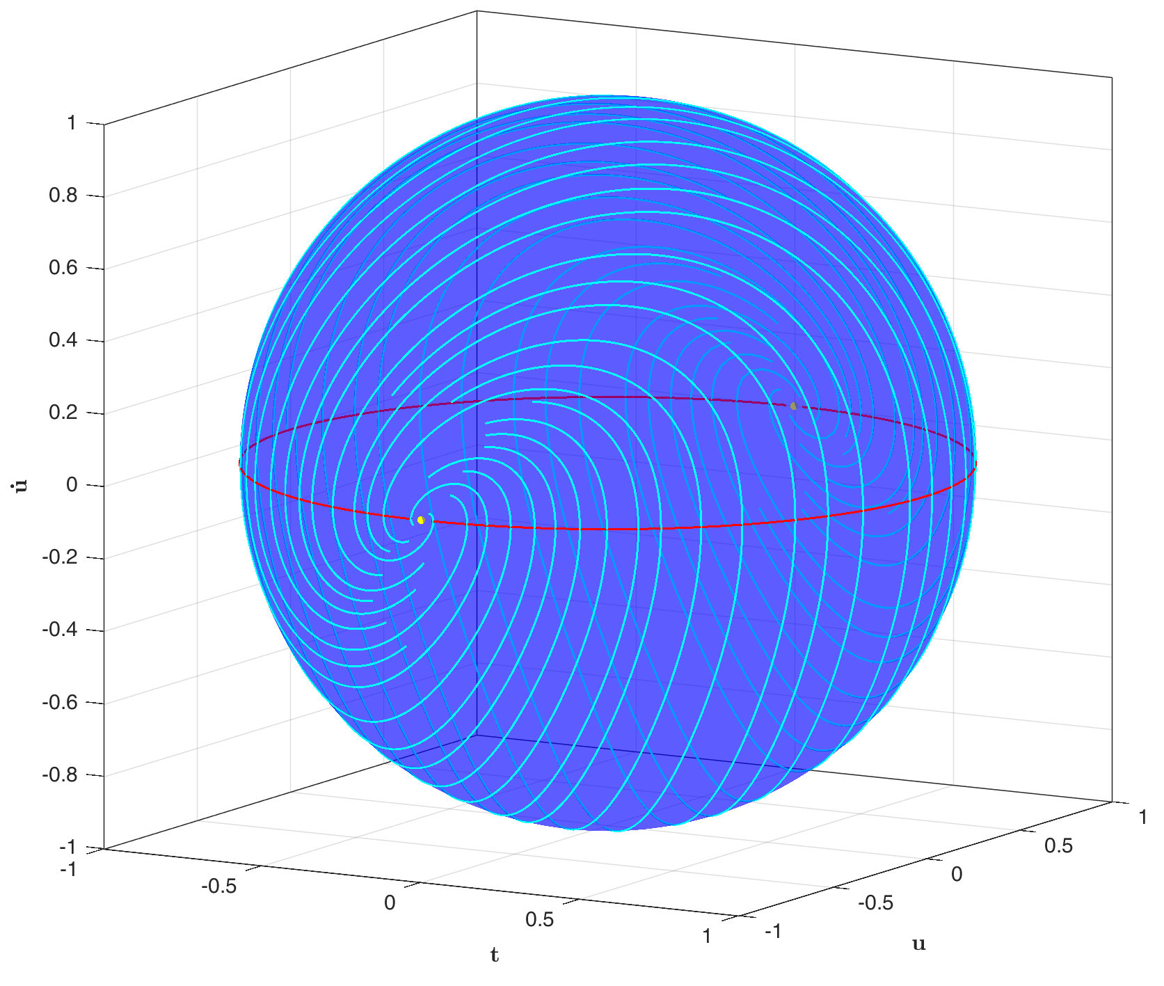
Figure 2. Unit sphere as semialgebraic differential equation

For systems containing equations of different orders or for systems obtained by prolongations, the following observation (which may be considered as a variation of [41, Prop. 9.5.10]) is useful, as it significantly reduces the size of the linear system (1). It requires that the system is well prepared, as it crucially depends on the fact that no hidden integrability conditions are present.

Proposition 11.

Let $\mathcal{J}_{\ell}\subset J_{\ell}\pi$ be a well-prepared basic semialgebraic differential equation of order $\ell$. Then it suffices to consider in the linear system (1) only those equations $p_{i}=0$ which are of order $\ell$; all other equations contribute only zero rows.

Proof.

By a slight abuse of notation (more precisely, by omitting some pull-backs), we have the following relation between the generators of the contact distributions of two neighbouring orders:

$$C^{(k+1)}_{\mathrm{trans}}=C^{(k)}_{\mathrm{trans}}+\sum_{\alpha=1}^{m}u_{\alpha}^{(k+1)}C^{(k)}_{\alpha}\,.$$

On the other hand, if $\varphi$ is any function (not necessarily polynomial) depending only on jet variables up to an order $k<\ell$, then its formal derivative is given by $D\varphi=C^{(k+1)}_{\mathrm{trans}}(\varphi)$. Since we assume that $\mathcal{J}_{\ell}$ is well prepared, for any equation $p_{i}=0$ in the corresponding basic semialgebraic system of order $k<\ell$ the prolonged equation $Dp_{i}=0$ can be expressed as a linear combination of the equations contained in the system (otherwise we would have found a hidden integrability condition). Because of $k<\ell$, we have $Dp_{i}=C^{(k+1)}_{\mathrm{trans}}(p_{i})=C^{(\ell)}_{\mathrm{trans}}(p_{i})$ and trivially $C^{(\ell)}_{\alpha}(p_{i})=0$ for all $\alpha$. Hence the row contributed by $p_{i}$ to (1) is a zero row, as $Dp_{i}(\rho)=0$ at any point $\rho\in\mathcal{J}_{\ell}$. ∎

For the purpose of detecting all geometric singularities in a given semialgebraic differential equation $\mathcal{J}_{\ell}$, we must analyse the behaviour of (1) in dependency of the point $\rho$. Thus we must now consider the coefficients of (1) as polynomials in the jet variables $(t,\mathbf{u},\mathbf{\dot{u}},\dots,\mathbf{u}^{(\ell)})$ and not as real numbers. Furthermore, we must augment (1) by the semialgebraic differential system defining $\mathcal{J}_{\ell}$ and study the combined system of equations and inequalities in the variables $(t,\mathbf{u},\mathbf{\dot{u}}\dots,\mathbf{u}^{(\ell)},a,\mathbf{b})$. In the approach of [33], one simply performs an algebraic Thomas decomposition of this system for a suitable ranking of the variables. While this approach is correct and identifies all geometric singularities, it has some shortcomings. It does not really exploit that a part of the problem is linear and as it implicitly also determines an algebraic Thomas decomposition of the differential equation $\mathcal{J}_{\ell}$, it leads in general to many redundant case distinctions, which are unnecessary for solely detecting all real singularities, but simply reflect certain geometric properties of the semialgebraic set $\mathcal{J}_{\ell}$.

We propose now as a novel approach to study the linear part (1) separately from the underlying semialgebraic differential equation $\mathcal{J}_{\ell}$ considering it as a parametric linear system in the unknowns $a$, $\mathbf{b}$ with the jet variables $(t,\mathbf{u},\mathbf{\dot{u}}\dots,\mathbf{u}^{(\ell)})$ as (yet independent) parameters. Using parametric Gaussian elimination, all possible different cases for the linear system are identified. Then, in a second step, it is verified for each case whether it occurs somewhere on the differential equation $\mathcal{J}_{\ell}$, i. e. we take now into account that our parameters are not really independent but have to satisfy a basic semialgebraic system. If yes, we obtain by simply combining the equations and inequalities describing the case distinction with the equations and inequalities defining $\mathcal{J}_{\ell}$ a semialgebraic description of the corresponding subset of $\mathcal{J}_{\ell}$.

According to Proposition 8, the coefficient matrix $A$ of the linear system (1) possesses the same rank at regular and at regular singular points. The difference between the two cases is the relative position of the Vessiot space to the linear subspace $W=\ker{T}_{\rho}\pi^{\ell}$: as one can see in Definition 4, at regular singular points the solution space lies in $W$, whereas at regular points its intersection with $W$ is trivial. For this reason, we need a parametric Gaussian elimination in the form developed in the previous section which takes the relative position of the solution space to a prescribed linear (cartesian) subspace into account. In terms of the $m+1$ coefficients $a$, $\mathbf{b}$ of our ansatz, $W$ corresponds to the cartesian subspace of $\mathbbm{R}^{m+1}$ defined by the equation $a=0$ (which we can write as $\Pi_{a}(\mathbbm{R}^{m+1})$ in the notation of the last section) and thus we solve (1) using Algorithm 1 with the choice $\mathbf{y}=(a)$. This means that – among the points with a one-dimensional solution space – we characterise the regular points as those where $a$ is the free variable in our solution representation and the regular singular points as those where $a=0$, i. e. where the intersection of the solution space of (1) with $\Pi_{a}(\mathbbm{R}^{m+1})$ is trivial.

Because of our special form of parametric Gaussian elimination and the choice of $\mathbf{y}=(a)$, all points on one of the obtained subsets $G(\Gamma_{i})$ are of the same type in the sense of Definition 4. The type is easy to decide on the basis of the form of the obtained row echelon form of the linear system (or of its solution) on the subset. Hence we do actually more than just detecting singularities: we identify semialgebraic subsets of $\mathcal{J}_{\ell}$ on which the Vessiot spaces allow for a uniform description and possess uniform properties. This is of great importance for a possible further analysis of the found singularities (not discussed here).

In a more formal language, our novel approach translates into Algorithm 2, the correctness of which follows from the above discussion. Note that for computational purposes we limit ourselves to input with integer coefficients. The critical steps are the parametric Gaussian elimination which may potentially lead to many case distinctions, but which represents otherwise a linear operation. For each obtained case, an existential closure must be studied to check whether the case actually occurs on $\mathcal{J}_{\ell}$. The real quantifier elimination in Redlog primarily uses virtual substitution techniques [31, 47, 48, 54, 55] and falls back into partial cylindrical algebraic decomposition [10, 11, 40] for subproblems where degree bounds are exceeded. The latter algorithm is double exponential in the worst case [9]. It is noteworthy that for our special case of existential sentences also single exponential algorithms exist [23] but no corresponding implementations.

Algorithm 2 RealSingularities

0:  well-prepared, basic semialgebraic system $\Sigma_{\ell}=\bigl{(}(p_{a}=0)_{a=1,\dots,A},(q_{b}>0)_{b=1,\dots,B}\bigr{)}$, where $p_{a}$, $q_{b}\in\mathcal{D}_{\ell}=\mathcal{D}\cap\mathbbm{Z}[t,\mathbf{u},\dots,\mathbf{u}^{(\ell)}]$

0:  finite system $(\Gamma_{i},\mathrm{H}_{i})_{i=1,\dots,I}$ with

1. each $\Gamma_{i}$ is a disjunctive normal form of polynomial equations, inequations, and inequalities over $\mathcal{D}_{\ell}$ describing a semialgebraic subset $\mathcal{J}_{\ell,i}\subseteq\mathcal{J}_{\ell}$

2. each $\mathrm{H}_{i}$ describes the Vessiot spaces of all points on $\mathcal{J}_{\ell,i}$

3. all sets $\mathcal{J}_{\ell,i}$ are disjoint and their union is $\mathcal{J}_{\ell}$

1:  set up the matrix $A$ of the linear system (1) using the equations $(p_{a}=0)_{a=1,\dots,A}$

2:  $\Pi=\bigl{(}\gamma_{\tau},\mathrm{H}_{\tau}\bigr{)}_{\tau=1,\dots,t}:=\mathtt{ParametricGauss}\bigl{(}A,(\mathbf{b},a),(a),\mathbbm{R}\bigr{)}$

3:  for $\tau:=1,\dots,t$ do

4:     let $\Gamma_{\tau}$ be a disjunctive normal form of $\gamma_{\tau}\land\bigwedge\Sigma_{\ell}$

5:     check satisfiability of $\Gamma_{\tau}$ using real quantifier elimination on $\exists t\,\exists\mathbf{u}\dots\exists\mathbf{u}^{(\ell)}\,\Gamma_{\tau}$

6:     if $\Gamma_{\tau}$ is unsatisfiable then

7:        delete $(\gamma_{\tau},\mathrm{H}_{\tau})$ from $\Pi$

8:     else

9:        replace $(\gamma_{\tau},\mathrm{H}_{\tau})$ by $(\Gamma_{\tau},\mathrm{H}_{\tau})$ in $\Pi$

10:     end if

11:  end for

12:  return $\Pi$

Remark 12.

It should be noted that the form of the guards $\Gamma_{i}$ appearing in the output is not uniquely defined. We produce a disjunctive normal form, as it is easier to interpret. However, many equivalent expressions can be obtained by performing some simplification steps and in particular by trying to factorise the polynomials appearing in the clauses. In the fairly simple examples considered in the next section, we always obtained an “optimal” form where no clause can be simplified any more. In larger examples, this will not necessarily be the case and it is non-trivial to define what “optimal” actually should mean.

Remark 13.

Many differential equations arising in applications depend on parameters $\boldsymbol{\chi}$, i. e. the polynomials $p_{a}$ and $q_{b}$ defining the equations and inequalities of the corresponding basic semialgebraic system depend not only on the jet variables $(t,\mathbf{u},\dots,\mathbf{u}^{(\ell)})$, but in addition on some real parameters $\boldsymbol{\chi}$. Such situations can still be handled by Algorithm 2. A straightforward solution consists of considering the parameters as additional unknown functions $\mathbf{u}$ and adding to the given semialgebraic system the differential equations $\dot{\boldsymbol{\chi}}=0$ (of course, one can this way also incorporated easily conditions on the parameters like positivity constraints by adding corresponding inequalities).

However, it is easier to apply directly Algorithm 2 with only some trivial modifications. We consider $p_{a}$ and $q_{b}$ as elements of the polynomial ring $\mathcal{D}_{\ell}[\boldsymbol{\chi}]$. For the parametric Gaussian elimination, there is no difference between the parameters $\boldsymbol{\chi}$ and the jet variables $(t,\mathbf{u},\dots,\mathbf{u}^{(\ell)})$: all of them represent parameters of the linear system of equations (1) for the Vessiot spaces. Thus in the output of the elimination step, the guards $\gamma_{\tau}$ will now generaly depend on both the jet variables $(t,\mathbf{u},\dots,\mathbf{u}^{(\ell)})$ and the additional parameters $\boldsymbol{\chi}$, i. e. they will also be defined in terms of polynomials in $\mathcal{D}_{\ell}[\boldsymbol{\chi}]$. Hence the guards $\gamma_{\tau}$ returned in the second line of Algorithm 2 will be defined by such polynomials, too. In the fifth line, we still consider only the existential closure over the jet variables $(t,\mathbf{u},\dots,\mathbf{u}^{(\ell)})$. The outcome of the satisfiability check is now either “unsatisfiable” or a formula over the remaining parameters $\boldsymbol{\chi}$. The only change in the algorithm is that in the latter case we must augment $\Gamma_{\tau}$ by the obtained formula (and recompute a disjunctive normal form). Note that the guards produced by the parametric Gaussian elimination always consist only of equations and inequations. By contrast, the possibly appearing additional satisfiability conditions on the parameters $\boldsymbol{\chi}$ are produced by a quantifier elimination and can be arbitrary inequalities.

5. Computational Experiments

We will now study the practical applicability and quality of results of the approach developed in this article on several examples. To this end, we have realised a prototype implementation of Algorithm 1 and Algorithm 2 in Reduce [24, 25], which is not yet ready for publication. We chose Reduce because on the one hand it is an open-source general purpose computer algebra system, and on the other hand its Redlog package [18, 45, 46] provides a suitable infrastructure for computations in interpreted first-order logic as required by our approach. Although technically a “package”, Redlog establishes a quite comprehensive software system on top of Reduce. Systematically developed and maintained since 1995, it has received more than 400 citations in the scientific literature, mostly for applications in the sciences and in engineering. Its current code base comprises around 65 KLOC.

Our implementation of Algorithm 1 uses from Redlog fast and powerful simplification techniques for quantifier-free formulas over the reals for the realisation of a nontrivial deduction procedure $\vdash_{K}$. We specifically apply the standard simplifier for ordered fields originally described in [19, Sect. 5.2]; one notable improvement since is the integration of identification and special treatment of positive variables as a generalisation of the concept of positive quantifier elimination described in [49, 50]. Our implementation of Algorithm 2 uses – corresponding to line 5 – implementations of real quantifier elimination, specifically virtual substitution [31] and partial cylindrical algebraic decomposition [40] as a fallback option when exceeding degree limits for virtual substitution.

The presented examples were chosen for their simplicity allowing for any easy check of the results with hand calculations and for the possibility to apply also the complex algorithm of [33] for comparison purposes. They do not represent real benchmarks testing the feasibility of the presented approach for large scale problems. However, they already demonstrate the potential of our approach to concisely and explicitly provide interesting insights into the appearance of singularities of ordinary differential equations. On a standard laptop, the required computing times were on the scale of milliseconds. We will report timings for more serious problems elsewhere.

Example 14.

We continue with Example 10, the unit sphere as first-order differential equation $\mathcal{J}_{1}$, and show the results of an automatised analysis. Our implementation returns for the corresponding semialgebraic differential system $\Sigma_{1}=(\dot{u}^{2}+u^{2}+t^{2}-1=0)$ as input a list with three pairs:

$$(\Gamma_{1},\mathrm{H}_{1}) =\left(\dot{u}\neq 0\,\wedge\,\dot{u}^{2}+u^{2}+t^{2}-1=0,\,\{a=r_{1},\,b=-r_{1}(u+t\dot{u})^{-1}\}\right),$$

$$(\Gamma_{2},\mathrm{H}_{2}) =\left(t\neq 0\,\wedge\,u^{2}+t^{2}-1=0\,\wedge\,\dot{u}=0,\,\{a=0,\,b=r_{2}\}\right),$$

$$(\Gamma_{3},\mathrm{H}_{3}) =\left(t=0\,\wedge\,u^{2}-1=0\,\wedge\,\dot{u}=0,\,\{a=r_{3},\,b=r_{4}\}\right).$$

It is easily seen that each guard $\Gamma_{i}$ describes a semialgebraic subset $\mathcal{J}_{1,i}\subset\mathcal{J}_{1}$ and that these sets are pairwise disjoint. Each set $\mathrm{H}_{i}$ parametrises the Vessiot spaces at the points of $\mathcal{J}_{1,i}$ and one can easily read off their dimensions. At each point on $\mathcal{J}_{1,1}$, the dimension is clearly one, since $\mathrm{H}_{1}$ contains one free variable $r_{1}=a$. The dimension of the Vessiot space at each point of $\mathcal{J}_{1,2}$ is also one because of the free variable $r_{2}=b$, but as $\mathrm{H}_{2}$ comprises the equation $a=0$, the Vessiot spaces are everywhere vertical. The set $\mathrm{H}_{3}$ contains two free variables $r_{3}=a$, $r_{4}=b$ so that everywhere on $\mathcal{J}_{1,3}$ the dimension is two. According to Definition 4, the points on $\mathcal{J}_{1,1}$ are regular, the points on $\mathcal{J}_{1,2}$ regular singular and the two points on $\mathcal{J}_{1,3}$ irregular singular. Thus we exactly reproduce the result of the analysis by hand presented in Example 10.

Applying the complex analysis of [33] (more precisely, a Maple implementation of it provided by one of the authors of [33]) to this example, we find that the algebraic step yields five cases. One of them contains no real points at all. Furthermore, for the regular singular points an unnecessary case distinction is made by treating the two points $(\pm 1,0,0)$ as a special case. This distinction is not due to the behaviour of the linear system (1), but stems from an algebraic Thomas decomposition of the sphere. If we consider only the $\mathbb{R}$-rational points in each case and combine the two cases describing regular singular points, the result coincides with the one obtained here.

Thus, even in such a simple example consisting only of a scalar first-order equation, all the potential problems of applying the complex analysis of [33] to real differential equations already occur. We obtain too many cases. Some are completely irrelevant for a real analysis, as they do not contain real points (in some situations, it might be non trivial to decide whether a case contains at least some real points). Other cases are at least irrelevant for detecting singularities. Sometimes, the underlying case distinctions are important for a further analysis of the singularities, but often they are simply due to the Thomas decomposition and have no intrinsic meaning.

Example 15.

Dara [13] resp. Davydov [14] classified the possible singularities of generic scalar first order equations $F(t,u,\dot{u})=0$ providing normal forms for all arising cases. One distinguishes two classes: folded and gathered singularities, respectively. In this example, we consider the gathered class. It is characterised by the normal form

$$\dot{u}^{3}+\chi u\dot{u}-t=0$$ (3)

with a real parameter $\chi$. Values $\chi>0$ correspond to the hyperbolic gather, whereas values $\chi<0$ lead to the elliptic gather (classically, one considers $\chi=\pm 1$). Again, it is straightforward to analyse (3) by hand. The linear equation for the Vessiot distribution is given by

$$(-1+\chi\dot{u}^{2})a+(3\dot{u}^{2}+\chi u)b=0\,.$$

Thus the singularities lie on the parabola $3\dot{u}^{2}+\chi u=0$. In the hyperbolic case, we find two real irregular singularities at $(\mp 2/\sqrt{\chi^{3}},-3/\chi^{2},\pm 1/\sqrt{\chi})$ where both coefficients of the linear equation vanish; in the elliptic case no real irregular singularities exist (see Figure 3).

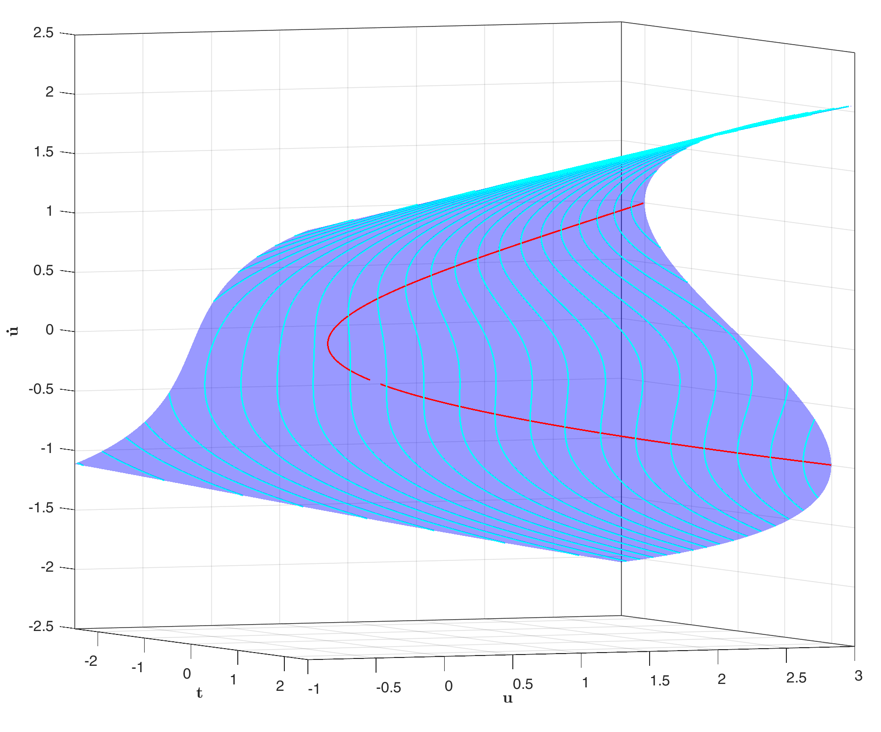
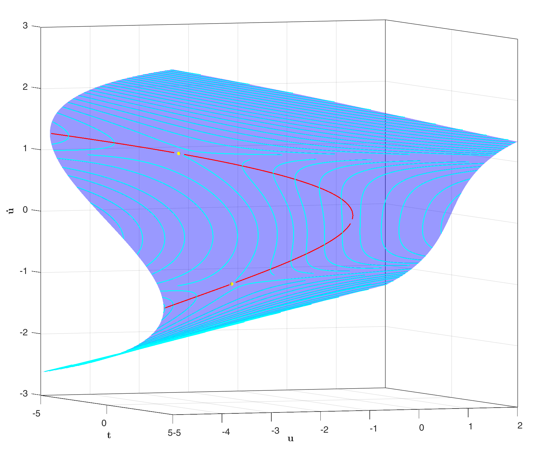
Figure 3. Elliptic and hyperbolic gather

Our implementation applied to the parametric differential equation (3) returns three pairs:

$$(\Gamma_{1},\mathrm{H}_{1}) =\left(3\dot{u}^{2}+\chi u\neq 0\,\wedge\,\dot{u}^{3}+\chi\dot{u}u-t=0,\,\{b=r_{1}(3\dot{u}^{2}+\chi u)^{-1}(1-\chi\dot{u}^{2}),\ a=r_{1}\}\right),$$

$$(\Gamma_{2},\mathrm{H}_{2}) =\left(\chi\dot{u}^{2}-1\neq 0\,\wedge\,3\dot{u}^{2}+\chi u=0\,\wedge\,\dot{u}^{3}+\chi\dot{u}u-t=0,\,\{a=0,\ b=r_{2}\}\right),$$

$$(\Gamma_{3},\mathrm{H}_{3}) =\left(3\dot{u}^{2}+\chi u=0\,\wedge\,\dot{u}^{3}+\chi\dot{u}u-t=0\,\wedge\,\chi\dot{u}^{2}-1=0\,\wedge\,\chi>0),\,\{a=r_{3},\ b=r_{4}\}\right).$$

As in the previous example, one can easily read off from the solutions $\mathrm{H}_{i}$ that the first case describes the regular points, the second case the regular singularities and the last case the irregular singularities. Note in the guard of the third case the clause $\chi>0$. It represents the solvability condition for the clause $\chi\dot{u}^{2}-1=0$ and distinguishes between the elliptic and the hyperbolic gather. In the elliptic gather the third case does not appear.

The results of a complex analysis are independent of the value of the parameter $\chi$. The algebraic Thomas decomposition yields seven cases: three with regular points, three with regular singularities and one with irregular singularities. One of the cases with regular singularities never contains a real point independent of $\chi$; the existence of real irregular singularities depends of course on the sign of $\chi$. The other unnecessary case distinctions stem again from an algebraic Thomas decomposition of the given equation.

So far, we have always studied each differential equation in the jet bundle of the order of the equation. However, in some cases it is also of interest to study prolongations, i. e. to proceed to higher order. This is e. g. necessary to see whether solutions of finite regularity exist (for a detailed analysis of a concrete class of quasilinear second-order equations in this respect see [42]). Obviously, the regularity of solutions is an issue only over the real numbers, as any holomorphic function is automatically analytic. A natural question is then whether there exists a maximal prolongation order at which all singularities can be detected. The following example due to Lange-Hegermann [32, Ex. 2.93] shows that this is not the case, as in it at any prolongation order something new happens. We make here contact with some classical (un)decidability questions for power series solutions of differential equations as e. g. studied in the classical article by Denef and Lipshitz [15].

Example 16.

We start with the first-order equation $\mathcal{J}_{1}\subset J_{1}\pi$ in three unknown functions $u$, $v$, $w$ of the independent variable $t$ defined by the following polynomial system:

$$tv\dot{u}-tu+1=0\,,\quad\dot{v}-w=0\,,\quad\dot{w}=0\,.$$ (4)

To obtain the first prolongation $\mathcal{J}_{2}\subset J_{2}\pi$, we must augment the system (4) by the equations

$$tv\ddot{u}+(tw+v-t)\dot{u}-u=0\,,\quad\ddot{v}=\ddot{w}=0\,.$$

If we prolong further to some order $q>2$, then for the definition of $\mathcal{J}_{q}\subset J_{q}\pi$ we must add for each integer $2<k\leq q$ the three equations

$$tvu^{(k)}+\bigl{[}(k-1)(tw+v)-t\bigr{]}u^{(k-1)}+(k-1)\bigl{[}(k-2)w-1\bigr{]}u^{(k-2)}=0\,,\quad v^{(k)}=w^{(k)}=0\,.$$

The Vessiot spaces of $\mathcal{J}_{1}$ arise as solutions of the linear system

$$(tw+v-t)\dot{u}a+tvb_{u}=0\,,\quad b_{v}=b_{w}=0\,.$$

For computing the Vessiot spaces of the prolonged equation, we exploit Proposition 11 telling us that at each prolongation order only the newly added equations must be considered. Hence we always obtain a linear system containing three equations. At any prolongation order $q>1$, the Vessiot spaces of $\mathcal{J}_{q}$ are defined by the linear system

$$\Bigl{[}\bigl{(}q(tw+v)-t\bigr{)}u^{(q)}+q\bigl{(}(q-1)w-1\bigr{)}u^{(q-1)}\Bigr{]}a+tvb_{u}=0\,,\quad b_{v}=b_{w}=0\,.$$

We fed the basic semialgebraic systems $\Sigma_{1}$, $\Sigma_{2}$ and $\Sigma_{3}$ corresponding to the first three equations $\mathcal{J}_{1}$, $\mathcal{J}_{2}$ and $\mathcal{J}_{3}$ into our implementation. For each system, it returned three cases containing the regular, regular singular and irregular singular points, respectively, of the corresponding differential equation. We obtained for $q=1$ the following results (we only discuss the guards $\Gamma_{i}$ and do not present the respective solutions $\mathrm{H}_{i}$). As already mentioned in Remark 9, the regular points represent the generic case and the corresponding guard is given by $\Gamma_{1}=(\Sigma_{1}\wedge v\neq 0\wedge t\neq 0)$. There is one family of regular singular points described by the guard

$$\Gamma_{2}=\bigl{(}\,\dot{w}=0\wedge\dot{v}-w=0\wedge tu-1=0\wedge v=0\wedge t(w-1)\dot{u}-u\neq 0\,\bigr{)}\,.$$

Obviously $v=0$ is the condition characterising singularities. The final inequation distinguishes the regular from the irregular ones: the guard $\Gamma_{3}$ for the latter one differs from $\Gamma_{2}$ only by this inequation becoming an equation. For later use, we make the following observation. The equation $tu-1=0$ implies that neither $t$ nor $u$ may vanish at a singularity. Thus at an irregular singularity we cannot have $w=1$ or $\dot{u}=0$, as otherwise the final equation in $\Gamma_{3}$ would be violated.

We refrain from explicitly writing down all the guards of the next prolongations, as they become more and more lengthy with increasing order. The regular points are always described by a guard of the form $\Gamma_{1}=(\Sigma_{q}\wedge v\neq 0\wedge t\neq 0)$. The key condition for singularities is always $v=0$. Besides the equations from $\Sigma_{2}$, the guard $\Gamma_{2}$ for the regular singularities of $\mathcal{J}_{2}$ contains in addition the equation $t(w-1)\dot{u}-u=0$ and the inequation $t(2w-1)\ddot{u}+2(w-1)\dot{u}\neq 0$ whereas for the irregular singularities this inequation becomes again an equation. Thus all the singularities of $\mathcal{J}_{2}$ lie over the irregular singular points of $\mathcal{J}_{1}$. This is not surprising, as it is easy to see that firstly for any differential equation $\mathcal{J}_{q}$ all singularities of its prolongation $\mathcal{J}_{q+1}$ must lie over the singularities of $\mathcal{J}_{q}$ and secondly that the fibre over a regular singular point is always empty. This time we can observe that at an irregular singularity we cannot have $w=1/2$ or $\ddot{u}=0$. The results of $\mathcal{J}_{3}$ are in complete analogy: now $w=1/3$ or $u^{(3)}=0$ are not possible at an irregular singularity.

The above made observations are of importance for the (non-)existence of formal power series solutions. Assume that we want to construct such a solution for the initial conditions $u(t_{0})=u_{0}$, $v(t_{0})=v_{0}$ and $w(t_{0})=w_{0}$. Recall that a point in the jet bundle $J_{q}\pi$ corresponds to a Taylor polynomial of degree $q$. Thus a point $\rho$ on a differential equation $\mathcal{J}_{q}$ may be considered as such a Taylor polynomial approximating a solution. This Taylor polynomial can be extended to one of degree $q+1$, if and only if the prolonged equation $\mathcal{J}_{q+1}$ contains at least one point lying over $\rho$. As already mentioned, this is never the case, if $\rho$ is a regular singularity. Hence, there can never exist a formal power series solution through a regular singular point. Our observations have now the following significance. Assume that we choose $v_{0}=0$ so that we are always at a singularity. Then no formal power series solution exists, if we choose $w_{0}=1$, as the $w$-coordinate of an irregular singularity of $\mathcal{J}_{1}$ can never have the value $1$. Similarly, no formal power series solutions exists for $w_{0}=1/2$, but now the problem occurs at the prolonged equation $\mathcal{J}_{2}$ where the $w$-coordinate of an irregular singularity can never have the value $1/2$. Generally, one can show by a simple induction that for $w_{0}=1/k$ with $k\in\mathbbm{N}$ no formal power series solution exists, as the prolongation $\mathcal{J}_{k}$ of order $k$ does not contain a corresponding irregular singularity.

Example 17.

As a final example, we study a minor variation of (4) which destroys most of the interesting properties of (4), but which nicely demonstrates why it is useful to take some care with how the guards are returned. We consider the following basic semialgebraic system which differs from (4) only by a missing factor $t$ in one term:

$$tv\dot{u}-u+1=0\,,\quad\dot{v}-w=0\,,\quad\dot{w}=0\,.$$ (5)

While our implementation yields for the regular points exactly the same guard as before, the dropped factor leads to considerable more distinct cases of regular and irregular singularities. The irregular singularities of $\mathcal{J}_{1}$ form the union of four two-dimensional (real) algebraic varieties, as one can easily recognise from the corresponding guard in disjunctive normal form:

$$\Gamma_{3}= (\,\dot{w}=0\wedge w-1=0\wedge\dot{v}-1=0\wedge v=0\wedge u-1=0\,)\vee{}$$

$$(\,\dot{w}=0\wedge\dot{v}-w=0\wedge v=0\wedge\dot{u}=0\wedge u-1=0\,)\vee{}$$

$$(\,\dot{w}=0\wedge\dot{v}-w=0\wedge v=0\wedge u-1=0\wedge t=0\,)\vee{}$$

$$(\,\dot{w}=0\wedge\dot{v}-w=0\wedge\dot{u}=0\wedge u-1=0\wedge t=0\,)\,.$$

The regular singularities form the union of two three-dimensional varieties without the above described union of four two-dimensional varieties. This set is characterised by the following guard in disjunctive normal form:

$$\Gamma_{2}= (\,\dot{w}=0\wedge\dot{v}-w=0\wedge v=0\wedge u-1=0\wedge w-1\neq 0\wedge\dot{u}\neq 0\wedge t\neq 0\,)\vee{}$$

$$(\,\dot{w}=0\wedge\dot{v}-w=0\wedge u-1=0\wedge t=0\wedge v\neq 0\wedge\dot{u}\neq 0\,)\,.$$

As in the last example, we also considered the first two prolongations of $\mathcal{J}_{1}$. The dimensions of the semialgebraic sets containing the regular, regular singular and irregular singular points are in any prolongation order $4$, $3$ and $2$. However, the guards $\Gamma_{2}$ and $\Gamma_{3}$ are getting more and more complicated. For $\mathcal{J}_{2}$ the guard $\Gamma_{2}$ contains four conjunctive clauses and $\Gamma_{3}$ six; for $\mathcal{J}_{3}$ these numbers raise to six and eight. Without some simplifications and the consequent transformation into disjunctive normal form, the guards would be much harder to read. The disjunctive normal form allows for a simple interpretation as union of basic semialgebraic sets (not necessarily disjoint).

6. Conclusions

For the basic existence and uniqueness theory of explicit ordinary differential equations, it makes no difference whether one works over the real or over the complex numbers. The standard proofs of the Picard–Lindelöf Theorem are independent of the base field. The situation changes completely, if one performs a deeper analysis of the equations and if one studies more general equations admitting singularities. Both the questions asked and the techniques used differ considerably over the real and over the complex numbers. We mentioned already in Section 5 the question of the regularity of solutions appearing only in a real analysis. There is a long tradition in studying the singularities of linear ordinary differential equations (see [53] for a rather comprehensive account of the classical results or [56] for an advanced modern presentation) and a satisfactory theory requires methods from complex analysis like monodromy groups and Stokes matrices. By contrast, singularities of nonlinear ordinary differential equations are mostly studied over the real numbers using methods from dynamical systems theory and differential topology (see [1, 36] for an introduction and [13, 14] for some typical classification results).

In this article, we were concerned with the algorithmic detection of all geometric singularities of a given system of algebraic ordinary differential equations. Using the geometric theory of differential equations, we could reduce this problem to a purely algebraic one. In [33], two of the authors presented together with collaborators a solution over the complex numbers via the Thomas decomposition. Now, we complemented the results of [33] by developing an alternative approach to the algebraic part of [33] (as the part where the base field really matters) applicable over the real numbers using parametric Gaussian elimination and quantifier elimination.

A key novelty of this alternative approach is to consider the decisive linear system (1) determining the Vessiot spaces first independently of the given differential system. This allows us to make maximal use of the linearity of (1) and to apply a wide range of heuristic optimisations. Compared with the more comprehensive approach of [33], this also leads to an increased flexibility and we believe that the new approach will be in general more efficient in the sense that fewer cases will be returned. Although we cannot prove this rigorously, already the comparatively small examples studied in Section 5 show this effect. We expect it to be much more pronounced for larger systems, as in the approach of [33] it cannot be avoided that the Thomas decomposition also analyses the geometry of a differential equation $\mathcal{J}_{\ell}$ even where it is irrelevant for the detection of singularities.

Our main tool for this first step is parametric Gaussian elimination. We proposed here a variant with two specific properties required by our application to differential equations. Firstly, it provides a disjoint partitioning of the parameter space. Secondly, it takes the relative position of the solution space with respect to a prescribed cartesian subspace taken into account. The last property was realised by an adapted pivoting strategy. Our elimination algorithm ParametricGauss makes strong use of a deduction procedure $\vdash_{K}$ for efficient heuristic tests for the vanishing or non-vanishing of certain coefficients under the current assumptions, thus avoiding redundant case distinctions at an early stage at comparatively little computational costs. The practical performance of the algorithm depends decisively on the power of this procedure. In our proof-of-concept realisation, we used with the Redlog simplifier a well-established powerful deduction procedure.

In the examples studied here, the results always turned out to be optimal in the sense that the output contained exactly three different cases corresponding to regular, regular singular and irregular singular points. In general, this will not be the case. In more complicated examples it may for instance happen that at different regular points different pivots are chosen by the parametric Gaussian elimination so that these points appear in different cases. Sometimes there may exist an intrinsic geometric reason for this, but sometimes these case distinctions may be simply due to the heuristics used to choose the pivots.

In the second step of our approach, the test whether the various cases found by the algorithm ParametricGauss actually appear on the analysed differential equation $\mathcal{J}_{\ell}$ requires a quantifier elimination. As in practice many algebraic differential equations are as polynomials of fairly low degree, fast virtual substitution techniques will often suffice. As fallback a partial cylindrical algebraic decomposition can be used.

We have ignored algebraic singularities, i. e. singular points in the sense of algebraic geometry. The Jacobian criterion allows us to identify them easily using linear algebra. In [33], the detection of algebraic and geometric singularities is done in one go. This approach leads again to certain redundancies, as among the algebraic singularities case distinctions are made because of the behaviour of the linear system (1), although the latter is not overly meaningful at such points. Our novel approach is more flexible and in it we believe that it makes more sense to separate the detection of the algebraic singularities from the detection of the geometric singularities.

One should note a crucial difference between the real and the complex case concerning algebraic singularities. On a complex variety, a point is nonsingular, if and only if a local neighbourhood of it looks like a complex manifold [29, Thm. 7.4]. For this reason, nonsingular points are often called smooth. Over the reals, one has no longer an equivalence: there may exist singular points on a real variety around which the variety looks like a real manifold [29, Rem. 7.8] [8, Ex. 3.3.12]. At such points, both the Zariski tangent space and the smooth tangent space are defined with the former being of higher dimension. For defining the Vessiot space at such a point, it appears preferable to use the smooth tangent space. However, it is a non-trivial task to identify such points. Diesse [16] presented recently a criterion for detecting them, but its effectivity is yet unclear. We will discuss elsewhere in more detail how one can cope with algebraic singularities over the reals.

References

- [1] V.I. Arnold. Geometrical Methods in the Theory of Ordinary Differential Equations. Springer, 2nd edition, 1988.
- [2] V.I. Arnold, S.M. Gusejn-Zade, and A.N. Varchenko. Singularities of Differentiable Maps I: The Classification of Critical Points, Caustics and Wave Fronts. Monographs in Mathematics 82. Birkhäuser, Boston, 1985.
- [3] F. Baader and T. Nipkow. Term Rewriting and All That. Cambridge University Press, 1998.
- [4] T. Bächler, V.P. Gerdt, M. Lange-Hegermann, and D. Robertz. Algorithmic Thomas decomposition of algebraic and differential systems. J. Symb. Comput., 47:1233–1266, 2012.
- [5] C. Ballarin and M. Kauers. Solving parametric linear systems: An experiment with constraint algebraic programming. ACM SIGSAM Bulletin, 38:33–46, 2004.
- [6] E.H. Bareiss. Sylvester’s identity and multistep integer-preserving Gaussian elimination. Math. Comp., 22(103):565–578, 1968.
- [7] E. Becker and R. Neuhaus. Computation of real radicals of polynomial ideals. In F. Eyssette and A. Galligo, editors, Computational Algebraic Geometry, Progress in Mathematics 109, pages 1–20. Birkhäuser, Basel, 1993.
- [8] J. Bochnak, M. Conte, and M.F. Roy. Real Algebraic Geometry. Ergebnisse der Mathematik und ihrer Grenzgebiete 36. Springer-Verlag, Berlin, 1998.
- [9] C.W. Brown and J.H. Davenport. The complexity of quantifier elimination and cylindrical algebraic decomposition. In Proc. ISSAC 2007, pages 54–60. ACM, 2007.
- [10] G.E. Collins. Quantifier elimination for the elementary theory of real closed fields by cylindrical algebraic decomposition. In Automata Theory and Formal Languages. 2nd GI Conference, volume 33 of LNCS, pages 134–183. Springer, 1975.
- [11] G.E. Collins and H. Hong. Partial cylindrical algebraic decomposition for quantifier elimination. J. Symb. Comput., 12:299–328, 1991.
- [12] D. Cox, J. Little, and D. O’Shea. Ideals, Varieties, and Algorithms. Undergraduate Texts in Mathematics. Springer-Verlag, New York, 4th edition, 2015.
- [13] L. Dara. Singularités génériques des équations différentielles multiformes. Bol. Soc. Bras. Mat., 6:95–128, 1975.
- [14] A.A. Davydov. Normal form of a differential equation, not solvable for the derivative, in a neighborhood of a singular point. Func. Anal. Appl., 19:81–89, 1985.
- [15] J. Denef and L. Lipshitz. Power series solutions of algebraic differential equations. Math. Ann., 267:213–238, 1984.
- [16] M. Diesse. On local real algebraic geometry and applications to kinematics. Preprint arXiv:1907.12134, 2019.
- [17] A. Dolzmann and T. Sturm. Guarded expressions in practice. In W. Küchlin, editor, Proc. ISSAC 1997, pages 376–383. ACM, 1997.
- [18] A. Dolzmann and T. Sturm. REDLOG: Computer algebra meets computer logic. ACM SIGSAM Bulletin, 31:2–9, 1997.
- [19] A. Dolzmann and T. Sturm. Simplification of quantifier-free formulae over ordered fields. J. Symb. Comput., 24:209–231, 1997.
- [20] V.P. Gerdt. On decomposition of algebraic PDE systems into simple subsystems. Acta Appl. Math., 101:39–51, 2008.
- [21] V.P. Gerdt, M. Lange-Hegermann, and D. Robertz. The MAPLE package TDDS for computing Thomas decompositions of systems of nonlinear PDEs. Comp. Phys. Comm., 234:202–215, 2019.
- [22] M. Golubitsky and V.W. Guillemin. Stable Mappings and Their Singularities. Graduate Texts in Mathematics 14. Springer-Verlag, New York, 1973.
- [23] D.Yu. Grigoriev. Complexity of deciding Tarski algebra. J. Symb. Comput., 5:65–108, 1988.
- [24] A.C. Hearn. Reduce—a user-oriented system for algebraic simplification. ACM SIGSAM Bulletin, 1:50–51, 1967.
- [25] A.C. Hearn. REDUCE: The first forty years. In A. Dolzmann, A. Seidl, and T. Sturm, editors, Algorithmic Algebra and Logic: Proceedings of the A3L 2005, pages 19–24. BOD, Norderstedt, Germany, 2005.
- [26] E. Hubert. Detecting degenerate behaviors in first order algebraic differential equations. Theor. Comp. Sci., 187:7–25, 1997.
- [27] M. Janet. Leçons sur les Systèmes d’Équations aux Dérivées Partielles. Cahiers Scientifiques, Fascicule IV. Gauthier-Villars, Paris, 1929.
- [28] U. Kant and W.M. Seiler. Singularities in the geometric theory of differential equations. In W. Feng, Z. Feng, M. Grasselli, X. Lu, S. Siegmund, and J. Voigt, editors, Dynamical Systems, Differential Equations and Applications (Proc. 8th AIMS Conference, Dresden 2010), volume 2, pages 784–793. AIMS, 2012.
- [29] K. Kendig. Elementary Algebraic Geometry. Graduate Texts in Mathematics 44. Springer-Verlag, New York, 1977.
- [30] E.R. Kolchin. Differential Algebra and Algebraic Groups. Academic Press, New York, 1973.
- [31] M. Košta. New Concepts for Real Quantifier Elimination by Virtual Substitution. Doctoral dissertation, Saarland University, Germany, 2016.
- [32] M. Lange-Hegermann. Counting Solutions of Differential Equations. PhD thesis, RWTH Aachen, Germany, 2014. Available at http://darwin.bth.rwth-aachen.de/opus3/frontdoor.php?source_opus=4993.
- [33] M. Lange-Hegermann, D. Robertz, W.M. Seiler, and M. Seiß. Singularities of algebraic differential equations. Preprint Kassel University (arXiv:2002.11597), 2020.
- [34] R. Neuhaus. Computation of real radicals of polynomial ideals II. J. Pure Appl. Alg., 124:261–280, 1998.
- [35] P.J. Olver. Applications of Lie Groups to Differential Equations. Graduate Texts in Mathematics 107. Springer-Verlag, New York, 1986.
- [36] A.O. Remizov. A brief introduction to singularity theory. Lecture Notes, SISSA, Trieste, 2010.
- [37] C. Riquier. Les Systèmes d’Équations aux Derivées Partielles. Gauthier-Villars, Paris, 1910.
- [38] J.F. Ritt. Differential Algebra. Dover, New York, 1966. (Original: AMS Colloquium Publications, Vol. XXXIII, 1950).
- [39] D. Robertz. Formal Algorithmic Elimination for PDEs. Lecture Notes in Mathematics 2121. Springer, Cham, 2014.
- [40] A. Seidl. Cylindrical Decomposition Under Application-Oriented Paradigms. Doctoral dissertation, Universität Passau, Germany, 2006.
- [41] W.M. Seiler. Involution: The Formal Theory of Differential Equations and its Applications in Computer Algebra. Algorithms and Computation in Mathematics 24. Springer, Berlin, 2010.
- [42] W.M. Seiler and M. Seiß. Singular initial value problems for scalar quasi-linear ordinary differential equations. Preprint Kassel University (arXiv:2002.06572), 2018.
- [43] W.Y. Sit. An algorithm for solving parametric linear systems. J. Symb. Comput., 13:353–394, 1992.
- [44] S. Spang. On the computation of the real radical. Diploma thesis, Technical University Kaiserslautern, Department of Mathematics, 2007.
- [45] T. Sturm. New domains for applied quantifier elimination. In Proc. CASC 2006, volume 4194 of LNCS. Springer, 2006.
- [46] T. Sturm. Redlog online resources for applied quantifier elimination. Acta Academiae Aboensis, Ser. B, 67(2):177–191, 2007.
- [47] T. Sturm. A survey of some methods for real quantifier elimination, decision, and satisfiability and their applications. Math. Comput. Sci., 11(3–4):483–502, 2017.
- [48] T. Sturm. Thirty years of virtual substitution. In Proc. ISSAC 2018, pages 11–16. ACM, 2018.
- [49] T. Sturm and A. Weber. Investigating generic methods to solve Hopf bifurcation problems in algebraic biology. In Proc. Algebraic Biology 2008, volume 5147 of LNCS, pages 200–215. Springer, 2008.
- [50] T. Sturm, A. Weber, E.O. Abdel-Rahman, and M. El Kahoui. Investigating algebraic and logical algorithms to solve Hopf bifurcation problems in algebraic biology. Math. Comput. Sci., 2(3):493–515, 2009.
- [51] J.M. Thomas. Differential Systems. Colloquium Publications XXI. AMS, 1937.
- [52] J.M. Thomas. Systems and Roots. W. Byrd Press, 1962.
- [53] W. Wasow. Asymptotic Expansions for Ordinary Differential Equations. Dover, New York, 1965.
- [54] V. Weispfenning. The complexity of linear problems in fields. J. Symb. Comput., 5:3–27, 1988.
- [55] V. Weispfenning. Quantifier elimination for real algebra—the quadratic case and beyond. Appl. Algebr. Eng. Comm., 8:85–101, 1997.
- [56] H. Żołądek. The Monodromy Group. Monografie Matematyczne 67. Birkhäuser, Basel, 2006.
Acknowledgments
This work was supported by the bilateral project ANR-17-CE40-0036 and DFG-391322026 SYMBIONT. The first two authors thank Marc Diesse for useful discussions about singularities in real algebraic geometry. The third author is grateful to Sarah Sturm at the University of Bonn and Marco Voigt at Max Planck Institute for Informatics for inspiring and clarifying discussions around Propositions 6 and 7.