SketchGNN: Semantic Sketch Segmentation with Graph Neural Networks

Abstract.

We introduce SketchGNN, a convolutional graph neural network for semantic segmentation and labeling of freehand vector sketches. We treat an input stroke-based sketch as a graph, with nodes representing the sampled points along input strokes and edges encoding the stroke structure information. To predict the per-node labels, our SketchGNN uses graph convolution and a static-dynamic branching network architecture to extract the features at three levels, i.e., point-level, stroke-level, and sketch-level. SketchGNN significantly improves the accuracy of the state-of-the-art methods for semantic sketch segmentation (by 11.2% in the pixel-based metric and 18.2% in the component-based metric over a large-scale challenging SPG dataset) and has magnitudes fewer parameters than both image-based and sequence-based methods.

1. Introduction

Freehand sketching is becoming one of the common interaction means between humans and machines with the continuous iteration of digital touch devices (e.g., smartphones, tablets) and various sketch-based interfaces on them. However, sketch interpretation still remains difficult for computers due to the inherent ambiguity and sparsity in user sketches, since sketches are often created with varying abstraction levels, artistic forms, and drawing styles. While many previous works attempt to interpret a whole sketch (Eitz et al., 2012a; Eitz et al., 2012b; Xu et al., 2013; Sangkloy et al., 2016; Li et al., 2020), part-level sketch analysis is increasingly required in multiple sketch applications (Sarvadevabhatla et al., 2017; Qi et al., 2015; Song et al., 2018; Xie et al., 2013; Li et al., 2016). In this article, we focus on semantic segmentation and labeling of sketched objects, an essential task in finer-level sketch analysis.

Lately, with the capacity of modern network architectures, deep-learning based sketch segmentation methods (Sarvadevabhatla et al., 2017; Li et al., 2019a; Zhu et al., 2019; Li et al., 2019c; Qi and Tan, 2019; Wu et al., 2018) have greatly improved the performance over traditional sketch segmentation methods (Delaye and Lee, 2015; Gennari et al., 2005; Schneider and Tuytelaars, 2016). These learning-based methods can be divided into two groups: image-based methods (Sarvadevabhatla et al., 2017; Li et al., 2019a; Zhu et al., 2019) and sequence-based methods (Li et al., 2019c; Qi and Tan, 2019; Wu et al., 2018). The image-based methods treat a sketch as a raster image and thus unavoidably ignore the stroke structure. In contrast, the sequence-based methods use relative coordinates of stroke points and pen actions to encode the stroke structure but neglect the proximity of points (especially among different strokes). The proximity information is crucial for sketch analysis according to the Gestalt laws (Wertheimer, 1938)).

SPGSeg (Li et al., 2019c)
FastSeg (Li et al., 2019a)
Ours
Human

Figure 1. Our graph-based method outperforms the state-of-art image-based metheod (FastSeg) and sequence-based method (SPGSeg), achieving a similar result to the manual labeling on the SPG Dataset.

To address the above issues with the existing solutions, we adopt the graph representation (Scarselli et al., 2009; Defferrard et al., 2016) to the sketch domain and present a novel method based on graph neural networks (GNNs). We treat a sketch as a 2D point set with certain graphical relationships automatically built from the original stroke structure. Our graph-based representation provides richer information against a raster image representation. Unlike sequence-based methods based on relative coordinates, our method uses the absolute coordinates of points, thus naturally providing the proximity. Furthermore, we introduce a novel Stroke Pooling operation to allow our network to aggregate stroke-level features in addition to point-level and sketch-level features, and greatly improve the consistency of labels within individual strokes.

Although the GNN-based method has the advantages compared to the other methods, semantic interpretation of sketches from the graphs built using the basic stroke structure (i.e., the static edges within individual strokes) is still challenging because of the resulting sparse graph structure. Schneider et al. (2016) manually add relation edges (e.g., proximity and enclosing relations) in the graph before using a Conditional Random Field (CRF). Their method, however is sensitive to variations of input. Inspired by the dynamic edges used in 3D point cloud analysis (Simonovsky and Komodakis, 2017; Valsesia et al., 2019; Wang et al., 2019), we use a similar technique in our network to extend the basic structure information. To alleviate the problem that dynamic edges may possibly bring wrong relationships between vertices and thus contaminate the original correct structure, we propose a two-branch network (Fig. 2): one branch using the original sparse structure and the other with dynamic edges, to balance the correctness and sufficiency.

Our main contributions are as follows: (1) We propose the first GNN-based method for semantic segmentation and labeling of sketched objects; (2) Our method significantly improves the accuracy of state-of-the-art and has magnitudes fewer parameters than both image-based methods and sequence-based methods.

2. Related work

Sketch Grouping

Sketch grouping divides strokes into clusters, with each cluster corresponding to an object part. Qi et al. (2013) treat this problem as a graph partition problem, and group strokes by graph cut. Later Qi et al. (2015) present a grouper that utilizes multiple Gestalt principles synergistically, with a novel multi-label graph-cut algorithm. Li et al. (2018b) and (2019c) use ordered strokes to represent a sketch, and develop a sequence-to-sequence Variational Autoencoder (VAE) model to learn a stroke affinity matrix. These methods, however, do not address the semantic labeling problem.

Semantic Sketch Segmentation

To semantically segment a sketch into groups with semantic labels, early works on sketch segmentation use hand-crafted features with limited ability to handle the large variations of sketches (Delaye and Lee, 2015; Gennari et al., 2005). Such user intervention (Noris et al., 2012; Perteneder et al., 2015) is often needed to achieve desired segmentation results. Later techniques (Huang et al., 2014; Schneider and Tuytelaars, 2016) leverage data-driven approaches to improve the accuracy of automatic segmentation. For example, Huang et al. (2014) use a mixed integer programming algorithm and utilize the segmentation information in a repository of pre-segmented 3D models. Schneider and Tyutelaars (2016) classify strokes based on Fisher vectors, build a graph by encoding relations between strokes, and finally use a Conditional Random Field (CRF) to solve for the most suitable label configuration. While these methods achieve reasonably accurate segmentation results, they are often computationally expensive.

The recent deep learning methods improve both the segmentation accuracy and the efficiency (Sarvadevabhatla et al., 2017; Li et al., 2019a; Zhu et al., 2019; Li et al., 2019c; Qi and Tan, 2019; Wu et al., 2018). The methods of (Sarvadevabhatla et al., 2017; Li et al., 2019a; Zhu et al., 2019) treat the sketch segmentation task as a semantic image segmentation problem and use convolutional neural networks (CNNs) to solve the problem. Such approaches usually ignore the structure information of strokes or use the stroke structure information in a post-processing step (Li et al., 2019a). In contrast, the methods of (Li et al., 2019c; Qi and Tan, 2019; Wu et al., 2018) treat the task as a sequence prediction problem. They use relative coordinates and pen actions to encode the structure information. However, sequence-based representations ignore the proximity of points. In contrast, our method uses a graph representation to fully exploit both the stroke structure and the stroke proximity, with carefully designed convolutional operations to extract both the intra-stroke and inter-stroke features.

Graph Neural Networks

Graph Neural Networks (GNNs) have been used in many applications for example for processing social networks (Tang and Liu, 2009), in recommendation engines (Monti et al., 2017; Ying et al., 2018), and in natural language processing (Bastings et al., 2017). GNNs are also suitable to process 2D and 3D point cloud data. Sketches are composed of strokes with ordered point sequences, making it possible to construct graphs based on strokes and to use GNNs for sketch segmentation. As far as we know, we are the first to apply GNNs to semantic sketch segmentation and labeling.

Graph structures in most GNNs are static. Recent studies about dynamic graph convolution show that changeable edges may perform better. For instance, filter weights in (Simonovsky and Komodakis, 2017) are dynamically generated for each specific data. EdgeConv in (Wang et al., 2019) dynamically computes node neighbors and constructs new graph structures in each layer. Valsesia et al. (2019) also construct node neighbors with the $k$-nearest neighbors (KNN) algorithm, in order to learn to generate point clouds. Since original graphs built from the stroke structure are very sparse, it is difficult to learn effective point-level features. To better capture global and local features, we will adopt a two-branch network and use both static and dynamic graph convolutions. Lately, Li et al. (2019b) leverage residual connections, dense connections, and dilated convolution to solve the problem of vanishing gradient and over-smoothing in GNNs (Li et al., 2018a; Kipf and Welling, 2016; Wu et al., 2019). Our method also exploits similar ideas when building our multi-layer GNNs.

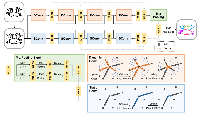
Figure 2. The architecture of our SketchGNN. An input sketch is first converted into a graph based on the stroke structure (the graph is simplified for illustration purpose). The graph node features and the connectivities are fed into the network, passing through two graph convolutional branches to extract the inter-stroke features (top, the global branch) and the intra-stroke features (bottom, the local branch). The extracted inter-stroke features are further fed into a mix pooling block to extract the global features, which are subsequently concatenated with the local features, and fed into a Multi-Layer Perceptron (MLP) to get the final results.

3. Overview

Fig. 2 shows the pipeline of our network. Given an input sketch, we first construct a graph from the basic stroke structure and use the absolute coordinate information as the features of the graph nodes (Section 4.1). Then the graph and the node features are fed into two branches (Section 4.2): a static branchconsists of several static graph convolutional units; a dynamic branchconsists of dynamic graph convolutional units and a mix pooling block (Section 4.3), including a max pooling operation and a stroke pooling operation. The learned features of two branches are concatenated and fed into a Multi-Layer Perceptron (MLP) to get the final segmentation and labeling.

The two-branch structure is tailored to the unique sketch structure, capturing both the intra-stroke information and the inter-stroke information. In the static branch, the information only flows inside individual strokes since different strokes are not connected in the input graph. We use this branch to generate point-level features. While in the dynamic-graph branch, we add extra connections with the nodes found by a dilated KNN ($k$ nearest neighbors) function. We use a mix-pooling block, more specifically, a max-pooling and a stroke-pooling after the dynamic graph convolutional units to aggregate both the sketch-level features and the stroke-level features, respectively. Experiments have proved that the design of such three-level features, i.e., point-level, sketch-level, and stroke-level (Section 4.3) is beneficial to our task compared with traditional two-level features, i.e., point-level and sketch-level (see Section 5.2).

4. Methodology

In this section, we first explain our graph-based sketch representation as input to the network. Then we introduce the two graph convolutional units separately used in two branches. followed by the descriptions of the three-level features.

4.1. Input Representation

Many existing sequence-based methods (Li et al., 2019c; Qi and Tan, 2019; Wu et al., 2018) use the relative coordinates to represent an input sketch. Instead, we use the absolute coordinates of sketch points, which are more suitable for our graph-based network structure.

Specifically, we represent a single sketch as an $N$-point set $\mathcal{P}={\{p_{i}=(x_{i},y_{i})\}}_{i=1,2,\cdots,{N}}$, where $x_{i}$ and $y_{i}$ are the 2D absolute coordinates of point $p_{i}$. A graph $\mathcal{G}$ is built using the basic stroke structure information, leading to a sparse graph $\mathcal{G}=(\mathcal{V},\mathcal{E})$, where $\mathcal{V}=\mathcal{P}$ and $\mathcal{E}$ includes the edges that connect adjacent points on each single stroke. We use the same input for both the static branch and the dynamic branchof our network.

4.2. Graph Convolutional Units

We use two types of graph convolutional units in our network: a static graph convolutional unit (SConv for short) in the static branchand a dynamic graph convolutional unit (DConv) in the dynamic branch. Both units use the same graph convolutional operation. The main difference between them is that the SConv unit does not update the graph connectivity during convolution in different layers while the DConv unit updates the graph connectivity layer by layer using KNN. Both units use residual connections, since their performance is more stable than the general connection (Xu et al., 2018b). We obtain the features $\mathcal{F}_{S}=\{f^{S}_{i}\}_{i=1,2,\cdots,{n_{s}}}$ after several SConv and the features $\mathcal{F}_{D}=\{f^{D}_{i}\}_{i=1,2,\cdots,{n_{d}}}$ after several DConv.

Graph Convolution Operation

We use the same graph convolution operation as in (Wang et al., 2019) and briefly explain the operation here for the convenience of reading. Given a graph at the $l$-th layer $\mathcal{G}_{l}=(\mathcal{V}_{l},\mathcal{E}_{l},\mathcal{F}_{l})$, where $\mathcal{V}_{l}$ and $\mathcal{E}_{l}$ are the respective vertices and edges in the graph $\mathcal{G}_{l}$, and $\mathcal{F}_{l}=\{f^{l}_{i}\}_{i=1,2,\cdots,n_{l}}$ is a set of node features, each defined at a vertex at the $l$-th layer.

The node feature $f^{l}_{i}$ of the vertex $v_{i}$ in the $l$-th layer is updated by

(1) $$f^{l}_{i}=\max_{j:(i,j)\in\mathcal{E}_{l}}h_{\Theta_{l}}(f^{l-1}_{i},f^{l-1}_{j}),$$

where $\Theta$ is the learnable weights of the feature update operation $h_{\Theta}(\cdot)$, and the operation is defined as

(2) $$h_{\Theta}(f_{i},f_{j})=\mathrm{ReLU}(\mathrm{MLP}_{\Theta}(concat(f_{i},f_{j}-f_{i}))).$$

Graph Updating Strategy

The SConv units only use the input graph and do not update the graph structure in different layers. In other words, we have $\mathcal{E}^{S}_{1}=\mathcal{E}^{S}_{2}=\cdots=\mathcal{E}^{S}_{l}=\mathcal{E}$ in the static branch. While the dynamic branchdynamically changes the graph by adding a different edge set $\mathcal{E}^{dyn}_{l}$ to the input graph in different layers, leading to non-local diffusion across the strokes. More specifically, the graph used in the $l$-th layer of the dynamic branchis defined as

(3) $$\mathcal{E}^{D}_{l}=\mathcal{E}\cup\mathcal{E}^{dyn}_{l}.$$

To enlarge the receptive fields, $\mathcal{E}^{dyn}_{l}$ is designed to get dilated aggregations of the information, inspired by Li et al. (2019b),

(4) $$\mathcal{E}^{dyn}_{l}=\{e_{ij}=\{v_{i},v_{j}\}|v_{j}\in\mathcal{K}^{(d)}(v_{i})\}_{i=1,\cdots,{N}}$$

where $\mathcal{K}^{(d)}(v_{i})$ is the $d$-dilated neighbors of vertex $v_{i}$. We use the same stochastic strategy at the training time as in (Li et al., 2019b).

4.3. Three-level Features

The features provided for the final MLP layer are composed of three parts: point-level features, stroke-level features, and sketch-level features. The point-level features $\mathcal{F}_{point}$ are obtained directly after several SConv units, meaning $\mathcal{F}_{point}=\mathcal{F}_{S}$.

A mix-pooling block, which contains two pooling operations is designed to learn the sketch-level features $\mathcal{F}_{sketch}=\{f_{i}^{sk}\}_{i=1,2,...,N}$ and the stroke-level features $\mathcal{F}_{stroke}=\{f_{i}^{st}\}_{i=1,2,...,N}$. Before applying two pooling operations, we transform the features $\mathcal{F}_{D}$ by using different multi-layer perceptrons with learnable weights $\Theta_{sk}$ and $\Theta_{st}$ separately.

We use the max pooling operation to aggregate the sketch-level features,

(5) $$f_{sk}=\max_{f_{i}\in\mathcal{F}_{D}}\mathrm{MLP}_{\Theta_{sk}}(f_{i})$$

and assign $f_{sk}$ for every point, i.e., $f^{sk}_{i}=f_{sk}$, similar to many existing methods used in 3D point cloud analysis (e.g., (Charles et al., 2017; Simonovsky and Komodakis, 2017)).

To compute the stroke-level features, we propose a novel pooling operation, named stroke pooling, to aggregate the features on every single stroke,

(6) $$f^{st}_{r}=\max_{j\in\mathcal{V}_{\mathcal{S}_{r}},f_{j}\in\mathcal{F}_{D}}\mathrm{MLP}_{\Theta_{st}}(f_{j}),$$

where $\mathcal{S}_{r}$ represents the $r$-th stroke in a sketch, and $\mathcal{V}_{\mathcal{S}_{r}}$ represents the vertex set of the stroke $\mathcal{S}_{r}$. The points in the same stroke gain the same stroke-level features $f^{stroke}_{i}=f^{st}_{r},i\in\mathcal{V}_{\mathcal{S}_{r}}$.

Therefore, the whole features used in the final MLP layers are a concatenation of the output of the dynamic branch (i.e., stroke-level feature $\mathcal{F}_{stroke}$ and sketch-level feature $\mathcal{F}_{sketch}$) and the output of the static branch(i.e., point-leval features $\mathcal{F}_{point}$):

(7) $$\mathcal{F}=concat(\mathcal{F}_{point},\mathcal{F}_{stroke},\mathcal{F}_{sketch}).$$

	SPGSeg (Li et al., 2019c)	FastSeg+GC (Li et al., 2019a)	Ours	Human
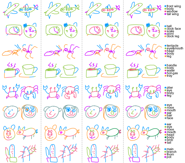
airplane
alarmclock
ant
coffeecup
crab
face
pig
cactus

Figure 3. Qualitative results of semantic segmentation on the SPG dataset. More visual results can be found in the appendix.

4.4. Implementation Details

Datasets

We run our SketchGNN on the following four existing sketch datasets: SPG dataset (Li et al., 2019c), SketchSeg-150K dataset (Wu et al., 2018), Huang14 dataset (Huang et al., 2014) and TU-Berlin dataset (Eitz et al., 2012a). The SPG and SketchSeg-150K datasets are both built upon QuickDraw (Ha and Eck, 2017), which is a vector drawing dataset selected from an online game where the players are required to draw objects in less than 20 seconds. SPG has 25 categories and 800 sketches per category and we use the same 20 categories as in (Li et al., 2019c). Compared to the SPG dataset, SketchSeg-150K is relatively simpler with fewer semantic labels per categories (2-4 labels per category). With data augmentation by a sketch generative model (Ha and Eck, 2017), SketchSeg-150K has about 150,000 sketches over 20 categories. The Huang14 dataset (Huang et al., 2014) and TU-Berlin dataset (Eitz et al., 2012a) are eariler smaller datasets which consist of 30 sketches and 80 sketches per category respectively. The specific statistics of the sketch datasets are presented in Table 1.

Table 1. Statistics of the number of labels per category and the number of storkes per sketch. The column Sketch shows the total number of sketches in different datasets in a form of $S\times C$, where $S$ represents the number of sketches per category and $C$ represents the number of categoies in every dataset.

Dataset	Sketch	strokes per sketch			labels per category
		min	max	median	min	max	median
SPG	800 $\times$ 20	2	43	6	3	8	4
150k	7500 $\times$ 20	1	7	3	2	4	3
Huang14	30 $\times$ 10	9	123	48	3	11	6
TUB	80 $\times$ 5	3	70	16	2	6	4

Network

As shown in Fig. 2, our network uses $L=4$ graph convolution units in both the local branch and the global branch. Each graph convolution unit computes edge features from connected point pairs by first concatenating point features and then using a multi-layer perceptron with the hidden size of $32$. Then it updates point features by aggregating neighboring edge features. In the global branch, we additionally use dynamic edges found by a dilated KNN function with the number of nearest neighbors $K=8$ and an increasing dilation rate $d=1,4,8,16$ for layers $0$ to $3$, respectively. In the mix pooling block, we apply a multi-layer perceptron with the hidden size of $128$ before each pooling operation. After pooling and repeating, the global features together with the local features are fed into a multi-layer perceptron with the hidden size of $[128,64,C]$ to get the final prediction.

Training

For SPG and SketchSeg-150K datasets, we directly split the original datasets to get the corresponding training and test sets. For Huang14 and TU-Berlin datasets, which have limited numbers of sketches per category, we make synthetic training data with labeled 3D models. We use the labeled 3D models provided by (Huang et al., 2014) for the Huang14 dataset and by (Yi et al., 2016) for the TU-Berlin dataset. We use the similar method of (Li et al., 2019a) to generate such synthetic data: we first render the normal maps of the 3D models using different colors for different segmentations, and then extract edge maps to approximate the sketch images by using the Canny edge detection algorithm (Canny and John, 1986). To obtain final vector sketch data, we design a simple algorithm for extracting stroke vectors from images: this algorithm randomly chooses one unprocessed pixel as the seed of a current stroke and searches its adjacent pixels to find the one having the minimum included angle with the current stroke direction as the next point. The stroke direction is initialized as the horizontal direction and updated when a new pixel is processed. Some intermediate results are shown in Fig. 4. We scale all sketches to fit a $256\times 256$ canvas. We then simplify each sketch using the Ramer-Douglas-Peucker algorithm (Douglas and Peucker, 1973) and resample it to $N$ points.

During the training phase, we use the cross-entropy loss and Adam ($\beta_{1}=0.9,\beta_{2}=0.999$) for optimization with the base learning rate $0.002$ and batch size $64$. For SPG and SketchSeg-150K, we train the network for 100 epochs and decay the rate by 0.5 for every 50 epochs. For Huang14 and TU-Berlin, we train the network for 30 epochs and decay the rate by 0.5 for every 10 epochs. The model is implemented with PyTorch and PyTorch Geometric, a geometric deep learning extension library for PyTorch. All models are trained with an NVIDIA GTX 1080Ti GPU. On average an epoch takes 15s on the SPG dataset and it takes 7ms to process a test sketch. We use $N=256$ for the SPG, Huang14, and TU-Berlin datasets, and $N=128$ for the SketchSeg-150K dataset, since the original sketches in the latter contain fewer points. During the test time, an input sketch is first resampled to $N$ points to pass through the network and then the predicted result is mapped back to the original sketch using a nearest-neighbor scheme.

Table 2. Quantitative comparisonon the SPG dataset (Li et al., 2019c). “P_metric” and “C_metric” stand for the pixel and component metrics, respectively. GC is short for graph cut refinement (Li et al., 2019a). “Ours w/o gt stroke” lists the results of our method by using the structure information automatically reconstructed from the raster images of the sketches in the dataset.

Category	SPGSeg (Li et al., 2019c)		DeepLab (Chen et al., 2018)		FastSeg+GC (Li et al., 2019a)		Ours		Ours w/o gt stroke
	P_metric	C_metric	P_metric	C_metric	P_metric	C_metric	P_metric	C_metric	P_metric	C_metric
airplane	82.9	70.9	70.7	46.2	85.3	75.2	96.4	92.3	91.8	86.7
alarm_clock	84.8	81.0	82.5	74.3	84.6	72.3	98.1	96.0	94.8	91.0
ambulance	80.7	68.1	72.5	54.2	85.8	75.3	94.2	90.3	89.2	83.0
ant	66.4	56.6	61.3	32.1	68.9	66.4	94.1	92.4	85.6	82.3
apple	89.9	71.8	87.3	60.2	91.4	82.3	97.2	93.4	94.3	88.4
backpack	75.2	63.7	64.3	28.4	73.3	59.8	92.7	86.7	84.8	77.4
basket	84.8	83.2	79.5	69.5	86.6	82.2	98.2	97.9	91.2	88.9
butterfly	89.0	83.6	85.6	69.8	92.7	79.3	99.6	98.7	96.3	94.7
cactus	77.5	72.3	67.2	30.8	73.3	68.6	97.5	96.5	92.7	80.7
calculator	91.1	89.9	92.5	92.1	97.4	93.0	99.3	99.0	98.7	95.1
campfire	92.3	91.4	82.9	83.3	95.6	92.9	97.3	96.0	90.3	87.8
candle	88.3	71.8	91.5	76.9	90.8	80.1	99.1	98.4	97.7	91.4
coffee cup	92.0	87.2	86.2	81.8	90.9	87.0	99.7	98.6	97.1	96.6
crab	77.9	70.5	73.9	49.3	75.9	55.4	96.1	94.0	91.7	87.5
duck	86.9	75.4	85.9	76.0	88.9	75.1	98.0	96.7	94.1	88.9
face	88.0	80.1	87.4	78.4	88.1	80.4	98.8	97.5	95.7	90.3
ice cream	85.4	79.3	80.7	70.3	87.5	80.1	95.2	95.3	89.9	85.3
pig	81.9	75.4	82.1	77.9	81.1	73.9	98.8	98.0	95.4	90.8
pineapple	89.8	90.2	85.4	79.5	91.9	82.3	98.8	96.5	94.5	90.7
suitcase	92.7	90.7	90.2	90.1	94.8	86.7	99.5	97.9	97.1	94.9
Average	84.9	77.6	80.5	59.0	86.2	77.4	97.4	95.6	93.1	88.6

Table 3. Quantitative comparison on the SketchSeg-150K dataset (Wu et al., 2018).

Category	FastSeg+GC (Li et al., 2019a)		SegNet+ (Wu et al., 2018)		Ours
	P_metric	C_metric	P_metric	C_metric	P_metric	C_metric
angel	0.98	0.96	0.89	0.86	0.99	0.98
bird	0.82	0.70	0.98	0.97	0.99	0.99
bowtie	1.00	1.00	0.99	1.00	1.00	1.00
butterfly	0.98	0.96	0.95	0.95	1.00	1.00
candle	0.96	0.78	0.95	0.95	0.98	0.97
cup	0.91	0.92	0.77	0.74	0.98	0.98
door	1.00	1.00	0.99	0.99	1.00	1.00
dumbbell	0.98	0.98	0.99	0.99	1.00	1.00
envelope	1.00	1.00	1.00	0.99	1.00	1.00
face	0.98	0.95	0.94	0.91	0.94	0.92
ice	1.00	1.00	0.72	0.69	1.00	1.00
lamp	0.78	0.78	0.95	0.94	0.96	0.96
lighter	0.99	0.96	0.99	0.98	1.00	1.00
marker	0.90	0.80	0.61	0.55	0.97	0.98
mushroom	0.98	0.94	0.70	0.66	0.99	0.94
pear	0.97	0.94	0.99	0.98	1.00	1.00
plane	1.00	0.99	0.86	0.85	1.00	1.00
spoon	0.80	0.79	0.85	0.81	0.90	0.90
traffic	0.89	0.93	0.96	0.96	0.95	0.95
van	0.99	0.99	0.87	0.84	0.99	0.99
Average	0.95	0.92	0.90	0.88	0.98	0.98

Table 4. Quantitative comparison on the Huang14 dataset (Huang et al., 2014).

Category	FastSeg (Li et al., 2019a)		FastSeg+GC (Li et al., 2019a)		DeepLab (Chen et al., 2018)		MIP-Auto (Huang et al., 2014)		Ours		Ours+GC
	P_metric	C_metric	P_metric	C_metric	P_metric	C_metric	P_metric	C_metric	P_metric	C_metric	P_metric	C_metric
airplane	81.1	65.4	85.5	75.5	45.0	30.4	74.0	55.8	80.0	66.6	82.9	75.4
bicycle	82.9	67.9	85.4	76.7	64.9	46.0	72.6	58.3	82.0	69.1	83.5	76.0
candelabra	74.7	59.2	77.3	68.0	58.6	44.1	59.0	47.1	78.6	66.7	81.4	74.3
chair	70.0	60.5	73.9	69.3	56.3	44.5	52.6	42.4	76.3	66.8	76.5	72.2
fourleg	79.6	66.5	83.9	75.8	64.6	49.1	77.9	64.4	80.2	67.8	82.0	74.9
human	74.8	61.9	79.2	71.9	67.6	55.5	62.5	47.2	75.5	66.3	76.5	71.0
lamp	85.7	78.1	86.5	80.9	68.3	64.8	82.5	77.6	87.1	79.2	89.8	86.5
rifle	68.5	56.3	71.4	67.3	63.8	50.2	66.9	51.5	77.9	67.4	79.3	73.3
table	77.6	67.3	79.0	73.1	64.6	51.9	67.9	56.7	78.6	68.0	81.0	76.7
vase	81.1	71.9	83.8	79.3	73.4	63.6	63.1	51.8	78.4	71.0	80.2	79.6
Average	77.6	65.5	80.6	73.8	62.7	50.0	67.9	55.3	79.5	69.2	81.3	76.0

Table 5. Quantitative comparison on subsets of the TU-Berlin dataset (Eitz et al., 2012a).

Category	FastSeg (Li et al., 2019a)		FastSeg+GC (Li et al., 2019a)		Ours		Ours+GC
	P_metric	C_metric	P_metric	C_metric	P_metric	C_metric	P_metric	C_metric
airplane	77.6	63.5	82.1	72.4	88.0	74.1	87.7	77.0
chair	91.7	89.5	95.7	93.5	95.5	92.5	95.9	93.7
guitar	78.5	67.0	81.4	78.8	91.6	86.0	92.5	87.7
motorbike	66.0	47.5	70.8	61.1	75.2	66.2	76.5	70.6
table	92.0	87.3	94.0	91.1	96.1	92.4	96.2	92.8
Average	81.2	71.0	84.8	79.4	89.3	82.2	89.8	84.4

5. Experiments

We evaluate our method on the aforementioned datasets and also compare our method to the current state-of-the-art sketch segmentation methods (Chen et al., 2018; Wu et al., 2018; Li et al., 2019a, c).

We perform both qualitative and quantitative comparisons. Fig. 1 and 3 show some representative visual comparisons between our method and the methods of (Li et al., 2019c) and (Li et al., 2019a) on the SPG dataset. The sequence-based method SPGSeg (Li et al., 2019c) uses point drawing orders and their relative coordinates but ignores the proximity among strokes, leading to unsatisfactory results (Fig. 2, the first column). The image-based method (Li et al., 2019a) is not aware of the stroke structure and hence mainly relies on the local image structure, also leading to inferior results.

5.1. Quantitative Evaluation

In this subsection, we discuss our quantitative comparisons on different datasets. For quantitative evaluation, we use the same evaluation metrics as the previous works (Huang et al., 2014; Li et al., 2019c; Wu et al., 2018; Li et al., 2019a):

• Pixel-based accuracy (P_metric), which evaluates the percentage of the pixels that are correctly labeled in all the sketches. The pixel metric is sensitive to label errors that appear on large components.

• Component-based accuracy (C_metric), which evaluates the percentage of the correctly labeled strokes, irrespective of the number of pixels in one stroke. A stroke is correctly labeled if at least 75% of its pixels have the correct label. The component metric is sensitive to label errors that appear on small components.

Table 2 lists the quantitative results of different methods on the SPG dataset. We use the same set of data split as in (Li et al., 2019c). Our approach outperforms others by a large margin: on average 11.2% higher in terms of the pixel metric and 18.2% higher in terms of the component metric on the SPG dataset than FastSeg + GC (Li et al., 2019a), which performs the best among the existing methods.

To validate the benefits of stroke structure, we test our model on a reconstructed SPG dataset, in which the stroke structure is derived from the rasterized images of the sketches. Specifically, we render the vector sketches to the binary images and rebuild the vector sketches by the stroke-extraction algorithm similar to the one we used in making the synthetic data for Huang14 and TU-Berlin datasets (Section 4.4). Considering the ambiguity of the reconstructed stroke structure, we evaluate the segmentation results on the original stroke structure after mapping the predicted label to the nearest point in the original sketch. The results of our method on this reconstructed SPG dataset are listed in Table 2 (the column ‘Ours w/o gt stroke’). With the stroke structure automatically inferred from the raster sketch images, our model still raises 6.9% on average in terms of the pixel metric and 11.2% on average in terms of the component metric compared with FastSeg + GC (Li et al., 2019a). This indicates that our method is potentially beneficial for semantic segmentation of raster sketch images.

Table 3 shows the comparison results on the SketchSeg-150K datasets with the same data split as in (Wu et al., 2018). Our approach exceeds FastSeg + GC (Li et al., 2019a) 3% higher in the pixel metric and 6% higher in the component metric on average. The less significant performance gain by our method on the SketchSeg-150K dataset than the SPG dataset is mainly because this dataset is labeled coarsely with fewer semantic labels per category (2-4 labels per category in SketchSeg-150K versus 3-7 labels per category in SPG) and thus less challenging for the existing methods.

We also evaluate our model on the Huang14 dataset and a subset of TU-Berlin dataset. Tables 4 and 5 show the respective quantitative results. In the Huang14 dataset, the individual strokes typically contain many spacious small segments (e.g., see Fig. 4, top row). Such small segments would potentially increase the structural noise and thus degrade the performance of our DConv units, since DConv connects new edges within the feature space. For a fair comparison, we apply an additional graph cut algorithm to refine our results as in (Li et al., 2019a). The situation is improved (see statistics in Table 5) in the TU-Berlin dataset where there are not many such spacious small segments, which indicates that our model can learn the stroke structure information. We did not include the results of our method with graph cut when comparing to existing methods on the SPG and SketchSeg-150K datasets, since GC did not bring any obvious improvements. Note GC is more helpful in (Li et al., 2019a) because their image-based method is not aware of the stroke structure and hence the prediction usually contains many spacious tiny segments within a single stroke (see details in (Li et al., 2019a)).

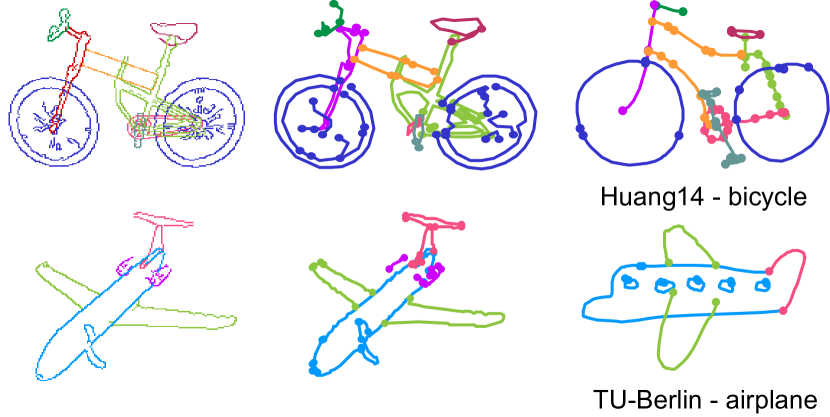
Figure 4. To create training data for the Huang14 and the TU-Berlin datasets, we construct graphs (Middle) from edge map images (Left) rendered from 3D models. The right column shows the exemplar freehand sketches in the test data. The synthesized and real sketches are different in both structure and shape. The endpoints of each stroke are marked with solid circles.

Overall, our method + GC gains on average 0.7% higher in the pixel metric and 2.2% higher in the component metric on the Huang14 dataset (than FastSeg + GC), and on average 5.0% higher in the pixel metric and 5.0% higher in the component metric on the TU-Berlin dataset. On the Huang14 dataset, our results are only slightly better than those by the CNN-based method FastSeg + GC (Li et al., 2019a) (in some categories even slightly worse, Table 4). This is mainly due to the large domain gap between the synthetic data rendered from 3D models and the real hand-drawn data, as shown in Fig. 4. The large domain gap may result in large structural noise for GNN-based methods to fully capture the stroke structures. Our method, however is still able to achieve the state-of-the-art performance.

It is noteworthy that compared with existing deep network-based models for sketch segmentation, our model has orders of magnitude fewer parameters. For example, the sequence-based method SPGSeg (Li et al., 2019c) has a parameter size of 23.4MB while the image-based method FastSeg + GC (Li et al., 2019a) has a parameter size of 40.9MB. In contrast, the parameter size of our model is only 434KB, which is two orders of magnitude tinier than them. However, the GNN model has some additional computation, such as for the aggregation of the vertices. We implement our model with PyTorch Geometric and achieve a similar runtime performance to the state-of-the-art method (FastSeg + GC(Li et al., 2019a)). The need of fewer parameters means that our model has more potential to be developed in light-weight applications like those on mobile devices.

Table 6. Quantitative results of ablation study on the SPG dataset. The baseline has only one dynamic branch and uses max pooling. B + D.S., B + D.D., and B + S.D. are the baseline with different combinations of two branches (S. and D. standing for the static and dynamic branches, respectively). B + S.P. is the baseline with stroke pooling. B + S.D. + S.P is our full model. We also show the simplified pipeline of each network for intuitive understanding. $\blacksquare$ and $\blacksquare$ represent the SConv and DConv blocks, respectively. $\blacksquare$ and $\blacksquare$ represent max-pooling and mix-pooling, respectively. $\blacksquare$ represents the input features and $\blacksquare$ represent the features sent into the final MLP.

	Baseline		B + D.S.		B + D.D.		B + S.D.		B + S.P.		B + S.D. + S.P.
Category	P	C	P	C	P	C	P	C	P	C	P	C
airplane	88.00	80.75	81.60	72.19	88.29	78.32	91.34	83.07	95.94	90.67	96.13	92.00
alarm_clock	92.15	86.79	88.69	81.08	90.74	84.98	93.82	89.57	97.57	95.04	97.99	96.08
ambulance	82.04	74.49	76.94	54.36	82.65	73.14	89.20	83.61	92.48	88.14	93.92	89.98
ant	82.70	78.55	76.80	66.81	84.35	78.09	87.93	83.65	90.30	89.21	94.12	92.42
apple	91.49	78.39	88.07	64.64	92.32	75.96	93.44	83.07	96.41	91.32	97.07	92.32
backpack	77.50	63.19	61.19	39.45	75.45	60.77	79.58	61.49	92.68	86.36	92.20	85.16
basket	82.12	76.60	80.92	74.25	84.40	76.41	83.42	77.49	97.52	97.13	97.75	97.32
butterfly	94.04	88.96	94.19	90.79	93.16	89.04	96.47	91.56	98.76	96.96	99.61	98.71
cactus	89.04	80.20	88.94	80.25	88.68	82.08	92.67	86.43	95.81	94.16	96.85	95.89
calculator	97.66	96.45	97.33	96.29	97.46	96.53	98.13	97.03	99.08	98.02	99.18	98.49
campfire	85.85	83.53	85.29	76.02	86.11	80.77	88.17	86.30	95.44	92.94	96.06	94.21
candle	96.40	91.52	96.23	87.61	96.23	89.29	97.73	95.19	99.17	97.98	99.14	98.35
coffee_cup	95.13	95.21	95.34	95.27	95.40	94.68	97.01	95.97	98.64	96.95	98.82	97.76
crab	89.02	82.61	86.90	78.97	88.10	82.75	92.43	86.67	95.03	92.43	96.08	94.01
duck	92.82	88.22	90.89	87.83	90.77	86.91	94.88	91.63	97.81	96.94	98.04	96.64
face	93.58	89.15	90.82	83.92	93.58	87.09	94.67	91.27	98.13	96.04	98.81	97.53
ice cream	86.39	82.29	84.94	79.52	85.44	77.04	89.78	84.16	94.62	92.55	95.21	95.32
pig	91.14	86.76	87.59	81.33	90.63	88.14	95.09	93.19	97.77	95.90	98.83	97.97
pineapple	92.01	89.55	88.76	85.02	92.67	88.63	96.13	92.00	98.69	95.80	99.03	96.45
suitcase	95.74	94.10	95.62	92.46	96.44	95.31	97.77	95.08	99.03	97.33	99.53	97.93
Average	89.74	84.37	86.85	78.40	89.64	83.30	92.48	87.42	96.54	94.09	97.22	95.23

Table 7. Quantitative results of GNN variants on the SPG dataset. SAGE-mean and SAGE-max are GraphSAGE with the mean and pooling aggregators, respectively. GIN-$\epsilon$ has a learnable parameter $\epsilon$ initialized with 0.1, while GIN-0 sets $\epsilon=0$.

Category	EdgeConv		MRGCN		SAGE-mean		SAGE-max		GIN-0		GIN-$\epsilon$		ECC
	P	C	P	C	P	C	P	C	P	C	P	C	P	C
airplane	96.6	92.5	95.1	91.2	93.5	88.3	94.6	89.9	95.1	89.8	94.1	88.7	94.2	87.2
alarm_clock	97.4	94.6	97.4	94.4	96.4	93.0	96.4	93.6	96.3	91.8	95.4	91.4	97.0	94.4
ambulance	93.5	90.1	94.0	90.2	92.9	89.0	90.8	85.4	91.3	86.5	92.2	88.1	92.1	87.9
ant	92.1	91.6	88.9	89.0	90.3	89.3	91.0	89.4	85.9	84.5	87.1	86.7	88.9	86.8
apple	96.4	90.7	97.1	93.1	95.9	89.9	89.9	73.7	96.0	88.7	96.6	90.4	95.8	88.8
…	…	…	…	…	…	…	…	…	…	…	…	…	…
Average	96.7	94.5	96.3	93.8	95.7	92.9	95.3	92.0	95.5	92.3	95.5	92.7	95.6	92.5

Table 8. Evaluation on different numbers of GCN units.

Average	4 units	6 units	8 units	10 units
P_metric	97.6%	96.9%	96.9%	96.7%
C_metric	95.6%	94.2%	94.2%	94.0%

Table 9. Evaluation on different values of N.

Average	128	256	512
P_metric	95.97%	96.62%	96.69%
C_metric	93.67%	94.44%	94.36%

5.2. Ablation Study

In this section we examine the effectiveness of our various design choices in SketchGNN. All the experiments are run on the SPG dataset since it has sufficient data and complexity. We use 650 sketches per category to train the models and choose the optimal model with the lowest average loss on the validation set with 50 sketches in 100 epoch training. The remaining 100 sketches are used as a test set to show the final performance.

Structure Design

We use the network with only the DConv units and the max-pooling aggregation as the baseline, which is a typical single-branch two-level-feature structure, similar to the network used in (Wang et al., 2019). Compared to the baseline, our model has two core improvements in structural design: 1) from two-level-feature to three-level-feature by adding the stroke-pooling operation; 2) from one-branch to two-branch by using both the static and dynamic graph convolutions.

Table 6 shows the benefit of these two designs: 1) With the stroke-pooling (i.e., S.P.), Base + S.P. outperforms the baseline by 6.8% in the pixel metric and 9.73% in the component metric; 2) With an additional static branch to generate the point-level features, Base + S.D. outperforms the baseline by 2.74% in the pixel metric and 3.06% in the component metric. To show the effectiveness of the two-branch structure we use, we design another two alternatives: the baseline with an additional dynamic branch (Base+D.D.) and the baseline with a static branch and a dynamic branch but use the SConv blocks before the pooling operation (Base+D.S.). Both of these networks are worse than Base+S.D.. Therefore, we use the baseline with an additional static branch and stroke-pooling as our full model (Base + S.D. + S.P.). Our full model achieves the best results: 7.48% better than the baseline in the pixel metric and 10.86% in the component metric.

GNN variants

For the choice of the convolution operation, we compare the effects of various GNN variants, including EdgeConv (Wang et al., 2019), MRGCN (Li et al., 2019b), GraphSAGE (Hamilton et al., 2017), GIN (Xu et al., 2018a), and ECC (Simonovsky and Komodakis, 2017). For ECC, we use $E(j,i)=({\delta}_{x},{\delta}_{y},\|\delta\|,\arctan{\delta}_{y}/{\delta}_{x})$ as its input edge features, where $\delta=p_{j}-p_{i}$ is the offset between two nodes, similar to their original design. Table 7 shows the experiments for the first 5 categories and the average results of the 20 categories on the SPG dataset. We use EdgeConv in our final model for its best performance in the experiments.

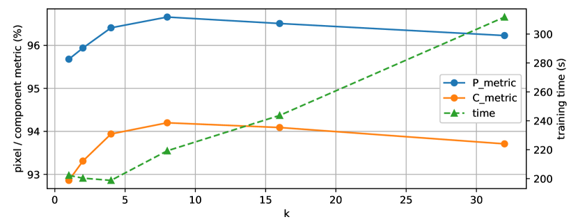
Figure 5. Evaluation of accuracy and efficiency with different values of K. The solid lines represent the evaluation results of two accuracy metrics. The dashed line represents the training time cost with different values of $K$.

The Number of GCN Units

We have tried alternating the number of GCN units used in our two branches. In our current setting, we use both 4 units (of SConv and DConv) in the global and the local branches. Alternatively, we change this number to 6, 8, and 10 convolutional units. As shown in Table 8, we find that increasing the number of GCN units does not benefit our results. For simplicity, we thus use 4 units in our final model.

The Number of Sample Points

We choose $N=256$ based on the complexity of sketches in the SPG dataset. With $N=256$, we will not lose the details of the original sketches. To investigate the impact of $N$, we also train the model with $N=128$ and $N=512$. Table 9 shows that using more points does not bring a significant improvement, while using fewer points reduces the performance.

The Value of K

In consideration of accuracy and efficiency, we choose $K=8$ when we build dynamic edges by the dilated KNN function. Generally, the larger the value of $K$, the longer the running time of the KNN algorithm. Fig. 5 shows that $K=8$ strikes a great balance between accuracy and efficiency. Note that the segmentation accuracy starts to drop gradually when $K$ is larger 8, possibly because the increased connection between the nodes causes an oversmoothing of the learned features.

Classification Test

In an interesting attempt, we try to use our model for the sketch recognition task with minor modifications. After we aggregate the features for every node according to Eq. 7, we apply MLP and average pooling on every point of sketches to get graph-level features. Such graph-level features are used to classify sketches by an MLP classifier. We run our experiments on the TU-Berlin dataset with 250 classes. However, the effect is not satisfying, with only a recognition accuracy of 52.3%. We suspect that the poor performance may be due to the different scales of the segmentation and recognition problems. According to Table 1, the maximum number of segmentation labels is 11, while the number of classification categories in TU-Berlin is 250. The model we design specifically for semantic segmentation might not have sufficient capacity to extract enough discriminating feature information for large-scale classification. We also perform the same classification experiment using the DGCNN model (Wang et al., 2019) with the default settings (except for $k=8$ to keep it the same as in our test), and the resulting classification accuracy is only 47.3%. The existing GNNs may have difficulty handling the sketch classification task for the sparse structure of sketches. Hence, for such tasks, further exploration is needed with GNNs in future work.

5.3. Invariance Test

To further demonstrate our method, we design invariance tests at three levels, i.e., sketch-level, stroke-level, and point-level. We perform the tests on four representative categories, i.e., Airplane, Calculator, Face, and Ice cream.

Sketch-level

Since we scale all sketches to fit a $256\times 256$ canvas, our method is not sensitive to translation or scaling. For the sketch-level invariance test, we apply random rotations to the sketches and monitor the segmentation results. Fig. 6 (Top) shows the results. It can be seen that as the range of the rotation angle increases, the performance decreases (dashed lines) rapidly if the training data does not contain similar sketches with random rotations. After we augment the training data with random rotations, the segmentation (solid lines) becomes more robust.

Point-level

For the point-level invariance test, we corrupt the input sketches with Gaussian noise. Specifically, we add random offset $O_{p}=(x_{o_{p}},y_{o_{p}})$ to every point in the sketch, where $x_{o_{p}},y_{o_{p}}\sim N(0,\delta^{2}),\delta=0,2,4,6,8,10$. It can be seen from Fig. 6 (Bottom) that training our model on the model with similar random noise can greatly improve the robustness of our method to random noise.

Stroke-level

For the stroke-level invariance test, we design three experiments.

In test I, we break the original strokes into small pieces. This changes the relationship of the points (the input graph) but not spatial layouts (i.e., the position) of the points (the input features). After partition, each new stroke contains up to $p_{s}$ vertices, where $p_{s}=\frac{10N}{2^{\psi}\cdot n_{s}}$, $\psi=1,2,3,4,5,6$, $N$ is the number of points in the sketch, and $n_{s}$ is the number of strokes in the sketch. Fig. 7 (Top) shows the results. The partition destroys the original stroke structure, causing poor segmentation results. When chopping up the strokes ($\psi=6$), the results become disastrous. Relevant data augmentation can help our model adapt to the broken strokes, as shown in Fig. 7. However, it cannot make the model extremely robust to such topological changes since the destroy of the stroke structure would undermine the benefit of the static-graph branch and stroke-pooling.

In test II, we add the random offset $O_{s}=(x_{o_{s}},y_{o_{s}})$ to every stroke in the sketch, where $x_{o_{s}},y_{o_{s}}\sim U(-\eta\times 256,\eta\times 256)$, $\eta=2\%,4\%,8\%,16\%,32\%$. In this setting, the position of points (the input features) has changed, but the relationship of the points (the input graph) remains the same. Fig.7 (Bottom) shows that data augmentation can improve the results but cannot eliminate the negative impact caused by the random offset since the random offset of the strokes can disrupt the learning of the relationship between the strokes. The experiment also shows that the correct inter-stroke relationships can benefit the segmentation task, and our model can learn such relationships.

Table 10. The component metric of our model and our model with two different data augmentation strategies on four representative categories.

C_metric	test w.o. scribbling			test w. scribbling
	Ours	Ours*	Ours**	Ours	Ours*	Ours**
airplane	92.3	93.1	93.5	82.6	93.9	91.8
calculator	99.0	97.4	98.3	96.0	97.7	97.5
face	97.5	96.5	96.2	94.1	96.7	94.8
ice cream	95.3	91.1	92.2	90.5	93.3	93.0

In test III, we scribble the sketch with meaningless strokes, leading to a decrease in the segmentation accuracy. Considering that re-sampling the sketch with scribbling stroke will change the original vertex position, we only use C_metric for quantitative analysis here. Some categories are not severely affected by scribbling, e.g., the Calculator (96.0% in C_metric, -3.0%). Some are severely affected, e.g., Airplane (82.6% in C_metric, -9.7%). We experiment with two strategies of data augmentation to combat the scribbling. One is to set another new label for the meaningless strokes (Ours*), and the other is to randomly assign one of the existing labelings to the meaningless strokes (Ours**) during the training stage. Table 10 shows that both strategies can work. On Category Airplane, the data augmentation even benefits the segmentation. Fig. 8 visualizes some segmentation results on Category Airplane in this experiment.

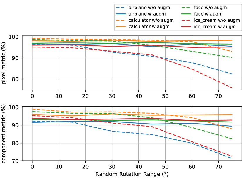
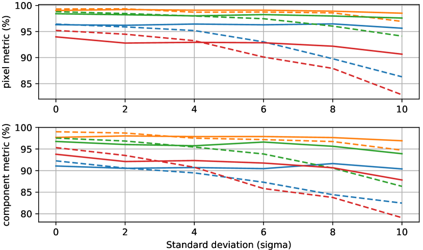
Figure 6. The visualization of the sketch-level invariance test (Top) and the point-level invariance test (Bottom) on four representative categories. The solid lines represent the evaluation results with data augmentation in the training stage, while the dashed lines represents those without data augmentation.

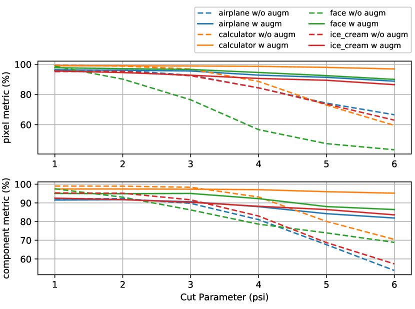
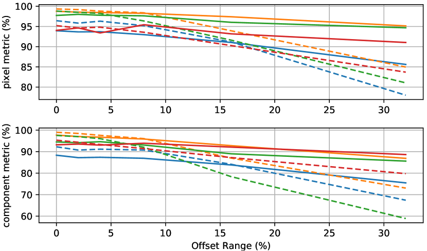
Figure 7. The visualization of two stroke-level invariance tests (Top for test I and Bottom for test II) on four representative categories. The solid lines represent the evaluation results with data augmentation in the training stage, while the dashed lines represents those without data augmentation.

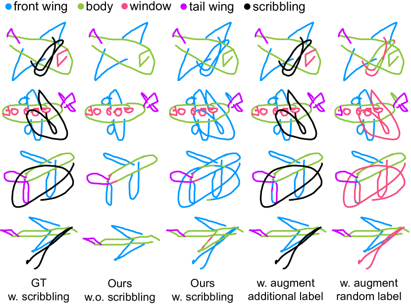
Figure 8. Representative results of stroke-level invariance test III on Category Airplane.

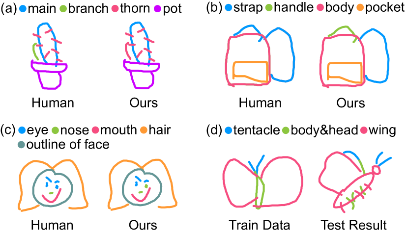
Figure 9. Exemplar results with imperfect segmentation.

6. Limitations

Fig. 9 shows several segmentation results with segmentation errors. The imperfection of our method is mainly caused by two factors. First, due to the inherent ambiguity of freehand sketches in part position and part shape, our model may assign wrong labels to strokes. For example, in Fig. 9 (a) the branch of the cactus is mistakenly assigned as thorn and (b) the strap on the top of a bag is labeled as handle. Second, the large differences between train data and test data may also mislead our model (Fig. 9 (d)): the butterflies in the train data always spread the wings, while the test example in this figure has the butterfly folded its wings, with a different view angle. We believe that the domain gap is a common issue of current learning based methods. Nevertheless, the visual results in Fig. 3 and the statistics on the Huang14 and the TU-Berlin datasets (Tables 4 and 5) have shown the generalization ability of our model. Finally, since our graph representation only warps features such as node position and proximity, our model is not aware of some high-level semantics such as the fact that “a human face can only have one nose” (see Fig. 9 (c)). We believe this issue can be alleviated by incorporating more semantic features into our graph representation for which we leave for future work.

7. Conclusion

In this work, we presented the first graph convolutional network for semantic sketch segmentation and labeling. Our SketchGNN employs static graph convolutional units and dynamic graph convolutional units to respectively extract intra-stroke and inter-stroke features using a two-branch architecture. With a novel stroke pooling operation enabling more consistent intra-stroke labeling, our method achieves higher accuracy than the state-of-the-art methods with significantly fewer parameters in multiple sketch datasets. In our current experiments, we only use absolute positions as graph node features, while ignoring the information of the stroke order, direction, spatial relation, etc. In the future, we will exploit these information with more flexible graph structures. Another possibility would be to exploit recurrent modules to learn intact graph representations. Finally, it could be an intriguing direction to reshape our architecture for scene-level sketch segmentation and sketch recognition tasks.

- (1)
- Bastings et al. (2017) Joost Bastings, Ivan Titov, Wilker Aziz, Diego Marcheggiani, and Khalil Sima’an. 2017. Graph Convolutional Encoders for Syntax-aware Neural Machine Translation. In Proceedings of the 2017 Conference on Empirical Methods in Natural Language Processing. 1957–1967.
- Canny and John (1986) Canny and John. 1986. A Computational Approach to Edge Detection. Pattern Analysis and Machine Intelligence, IEEE Transactions on (1986).
- Charles et al. (2017) R. Qi Charles, Su Hao, Kaichun Mo, and Leonidas J. Guibas. 2017. PointNet: Deep Learning on Point Sets for 3D Classification and Segmentation. In 2017 IEEE Conference on Computer Vision and Pattern Recognition (CVPR). 77–85.
- Chen et al. (2018) Liang-Chieh Chen, George Papandreou, Iasonas Kokkinos, Kevin Murphy, and Alan L. Yuille. 2018. DeepLab: Semantic Image Segmentation with Deep Convolutional Nets, Atrous Convolution, and Fully Connected CRFs. IEEE Trans. Pattern Anal. Mach. Intell. 40, 4 (2018), 834–848.
- Defferrard et al. (2016) Michal Defferrard, Xavier Bresson, and Pierre Vandergheynst. 2016. Convolutional Neural Networks on Graphs with Fast Localized Spectral Filtering. (2016).
- Delaye and Lee (2015) Adrien Delaye and Kibok Lee. 2015. A flexible framework for online document segmentation by pairwise stroke distance learning. Pattern Recognition 48, 4 (2015), 1197–1210.
- Douglas and Peucker (1973) David H. Douglas and Thomas K. Peucker. 1973. Algorithms for the reduction of the number of points required to represent a line or its caricature. University of Toronto Press.
- Eitz et al. (2012a) Mathias Eitz, James Hays, and Marc Alexa. 2012a. How Do Humans Sketch Objects? ACM Transactions on Graphics (Proceedings SIGGRAPH) 31, 4 (2012), 44:1–44:10.
- Eitz et al. (2012b) Mathias Eitz, Ronald Richter, Tamy Boubekeur, Kristian Hildebrand, and Marc Alexa. 2012b. Sketch-Based Shape Retrieval. ACM Transactions on Graphics (Proceedings SIGGRAPH) 31, 4 (2012), 31:1–31:10.
- Gennari et al. (2005) Leslie Gennari, Levent Burak Kara, Thomas F. Stahovich, and Kenji Shimada. 2005. Combining geometry and domain knowledge to interpret hand-drawn diagrams. Computers & Graphics 29, 4 (2005), 547–562.
- Ha and Eck (2017) David Ha and Douglas Eck. 2017. A Neural Representation of Sketch Drawings. In 6th International Conference on Learning Representations, ICLR 2018.
- Hamilton et al. (2017) William L. Hamilton, Rex Ying, and Jure Leskovec. 2017. Inductive Representation Learning on Large Graphs. In Proceedings of the 31st International Conference on Neural Information Processing Systems. 1025–1035.
- Huang et al. (2014) Zhe Huang, Hongbo Fu, and Rynson W. H. Lau. 2014. Data-driven Segmentation and Labeling of Freehand Sketches. ACM Trans. Graph. 33, 6 (2014), 175:1–175:10.
- Kipf and Welling (2016) Thomas N. Kipf and Max Welling. 2016. Semi-Supervised Classification with Graph Convolutional Networks. In International Conference on Learning Representations.
- Li et al. (2019b) Guohao Li, Matthias Müller, Ali Thabet, and Bernard Ghanem. 2019b. DeepGCNs: Can GCNs Go as Deep as CNNs?. In The IEEE International Conference on Computer Vision (ICCV).
- Li et al. (2018b) Ke Li, Kaiyue Pang, Jifei Song, Yi-Zhe Song, Tao Xiang, Timothy M. Hospedales, and Honggang Zhang. 2018b. Universal Sketch Perceptual Grouping. In The European Conference on Computer Vision (ECCV). 582–597.
- Li et al. (2019c) Ke Li, Kaiyue Pang, Yi-Zhe Song, Tao Xiang, Timothy M. Hospedales, and Honggang Zhang. 2019c. Toward Deep Universal Sketch Perceptual Grouper. IEEE Transactions on Image Processing 28, 7 (2019), 3219–3231.
- Li et al. (2019a) Lei Li, Hongbo Fu, and Chiew-Lan Tai. 2019a. Fast Sketch Segmentation and Labeling With Deep Learning. IEEE Computer Graphics and Applications 39, 2 (2019), 38–51.
- Li et al. (2016) Lei Li, Zhe Huang, Changqing Zou, Chiew-Lan Tai, Rynson W. H. Lau, Hao Zhang, Ping Tan, and Hongbo Fu. 2016. Model-driven sketch reconstruction with structure-oriented retrieval. In SIGGRAPH ASIA 2016 Technical Briefs. 28:1–28:4.
- Li et al. (2020) Lei Li, Changqing Zou, Youyi Zheng, Qingkun Su, and Chiew Lan Tai. 2020. Sketch-R2CNN: An RNN-Rasterization-CNN Architecture for Vector Sketch Recognition. IEEE Transactions on Visualization and Computer Graphics PP, 99 (2020), 1–1.
- Li et al. (2018a) Qimai Li, Zhichao Han, and Xiao-Ming Wu. 2018a. Deeper Insights Into Graph Convolutional Networks for Semi-Supervised Learning. In Proceedings of the Thirty-Second AAAI Conference on Artificial Intelligence. 3538–3545.
- Monti et al. (2017) Federico Monti, Michael Bronstein, and Xavier Bresson. 2017. Geometric Matrix Completion with Recurrent Multi-Graph Neural Networks. In Advances in Neural Information Processing Systems 30. 3697–3707.
- Noris et al. (2012) Gioacchino Noris, Daniel Sykora, A. Shamir, Stelian Coros, Brian Whited, Maryann Simmons, Alexander Hornung, Markus H. Gross, and Robert W. Sumner. 2012. Smart Scribbles for Sketch Segmentation. Computer Graphics Forum 31, 8 (January 2012).
- Perteneder et al. (2015) Florian Perteneder, Martin Bresler, Eva Maria Grossauer, Joanne Leong, and Michael Haller. 2015. cLuster: Smart Clustering of Free-Hand Sketches on Large Interactive Surfaces. In Proceedings of the 28th Annual ACM Symposium on User Interface Software and Technology. 37–46.
- Qi et al. (2013) Yonggang Qi, Jun Guo, Yi Li, Honggang Zhang, Tao Xiang, and Yi-Zhe Song. 2013. Sketching by perceptual grouping. In 2013 IEEE International Conference on Image Processing. 270–274.
- Qi et al. (2015) Yonggang Qi, Jun Guo, Yi-Zhe Song, Tao Xiang, Honggang Zhang, and Zheng-Hua Tan. 2015. Im2Sketch: Sketch generation by unconflicted perceptual grouping. Neurocomputing 165 (2015), 338–349.
- Qi et al. (2015) Yonggang Qi, Yi-Zhe Song, Tao Xiang, Honggang Zhang, Timothy Hospedales, Yi Li, and Jun Guo. 2015. Making Better Use of Edges via Perceptual Grouping. In 2015 IEEE Conference on Computer Vision and Pattern Recognition (CVPR). 1856–1865.
- Qi and Tan (2019) Yonggang Qi and Zheng-Hua Tan. 2019. SketchSegNet+: An End-to-End Learning of RNN for Multi-Class Sketch Semantic Segmentation. In IEEE Access, Vol. 7. 102717–102726.
- Sangkloy et al. (2016) Patsorn Sangkloy, Nathan Burnell, Cusuh Ham, and James Hays. 2016. The Sketchy Database: Learning to Retrieve Badly Drawn Bunnies. ACM Trans. Graph. 35, 4 (2016), 119:1–119:12.
- Sarvadevabhatla et al. (2017) Ravi Kiran Sarvadevabhatla, Isht Dwivedi, Abhijat Biswas, Sahil Manocha, and R. Venkatesh Babu. 2017. SketchParse : Towards Rich Descriptions for Poorly Drawn Sketches using Multi-Task Hierarchical Deep Networks. In Proceedings of the 25th ACM International Conference on Multimedia. 10–18.
- Scarselli et al. (2009) F. Scarselli, M. Gori, A. C. Tsoi, M. Hagenbuchner, and G. Monfardini. 2009. The Graph Neural Network Model. IEEE Transactions on Neural Networks 20, 1 (2009), 61–80.
- Schneider and Tuytelaars (2016) Rosália G. Schneider and Tinne Tuytelaars. 2016. Example-Based Sketch Segmentation and Labeling Using CRFs. ACM Trans. Graph. 35, 5 (2016), 151:1–151:9.
- Simonovsky and Komodakis (2017) Martin Simonovsky and Nikos Komodakis. 2017. Dynamic Edge-Conditioned Filters in Convolutional Neural Networks on Graphs. In 2017 IEEE Conference on Computer Vision and Pattern Recognition (CVPR). 29–38.
- Song et al. (2018) Jifei Song, Kaiyue Pang, Yi-Zhe Song, Tao Xiang, and Timothy M. Hospedales. 2018. Learning to Sketch with Shortcut Cycle Consistency. In 2018 IEEE Conference on Computer Vision and Pattern Recognition (CVPR). 801–810.
- Tang and Liu (2009) Lei Tang and Huan Liu. 2009. Relational Learning via Latent Social Dimensions. In Proceedings of the 15th ACM SIGKDD International Conference on Knowledge Discovery and Data Mining. 817–826.
- Valsesia et al. (2019) Diego Valsesia, Giulia Fracastoro, and Enrico Magli. 2019. Learning Localized Generative Models for 3D Point Clouds via Graph Convolution. In International Conference on Learning Representations.
- Wang et al. (2019) Yue Wang, Yongbin Sun, Ziwei Liu, Sanjay E. Sarma, Michael M. Bronstein, and Justin M. Solomon. 2019. Dynamic Graph CNN for Learning on Point Clouds. ACM Trans. Graph. 38, 5 (2019), 146:1–146:12.
- Wertheimer (1938) Max Wertheimer. 1938. Laws of Organization in Perceptual Forms. Psychologische Forschung 4 (1938), 71–88.
- Wu et al. (2018) Xingyuan Wu, Yonggang Qi, Jun Liu, and Jie Yang. 2018. Sketchsegnet: A Rnn Model for Labeling Sketch Strokes. In 2018 IEEE 28th International Workshop on Machine Learning for Signal Processing (MLSP). 1–6.
- Wu et al. (2019) Zonghan Wu, Shirui Pan, Fengwen Chen, Guodong Long, Chengqi Zhang, and Philip S. Yu. 2019. A Comprehensive Survey on Graph Neural Networks. CoRR abs/1901.00596 (2019). arXiv:1901.00596 http://arxiv.org/abs/1901.00596
- Xie et al. (2013) Xiaohua Xie, Kai Xu, Niloy Mitra, Daniel Cohen-Or, Wenyong Gong, Qi Su, and Baoquan Chen. 2013. Sketch-to-Design: Context-Based Part Assembly. Computer Graphics Forum 32 (11 2013), 233–245. https://doi.org/10.1111/cgf.12200
- Xu et al. (2018a) Keyulu Xu, Weihua Hu, Jure Leskovec, and Stefanie Jegelka. 2018a. How powerful are graph neural networks? arXiv preprint arXiv:1810.00826 (2018).
- Xu et al. (2013) Kun Xu, Chen Kang, Hongbo Fu, Wei-Lun Sun, and Shi-Min Hu. 2013. Sketch2Scene: Sketch-based Co-retrieval and Co-placement of 3D Models. Acm Transactions on Graphics (Proceedings SIGGRAPH) 32, 4 (2013), 1–15.
- Xu et al. (2018b) Keyulu Xu, Chengtao Li, Yonglong Tian, Tomohiro Sonobe, Ken Ichi Kawarabayashi, and Stefanie Jegelka. 2018b. Representation Learning on Graphs with Jumping Knowledge Networks. arXiv (2018).
- Yi et al. (2016) Li Yi, Vladimir G. Kim, Duygu Ceylan, I Chao Shen, Mengyan Yan, Hao Su, Cewu Lu, Qixing Huang, Alla Sheffer, and Leonidas Guibas. 2016. A scalable active framework for region annotation in 3D shape collections. ACM Transactions on Graphics (TOG) 35, 6cd (2016), 210.1–210.12.
- Ying et al. (2018) Rex Ying, Ruining He, Kaifeng Chen, Pong Eksombatchai, William L. Hamilton, and Jure Leskovec. 2018. Graph Convolutional Neural Networks for Web-Scale Recommender Systems. In Proceedings of the 24th ACM SIGKDD International Conference on Knowledge Discovery and Data Mining. 974–983.
- Zhu et al. (2019) Xianyi Zhu, Yi Xiao, and Yan Zheng. 2019. 2D freehand sketch labeling using CNN and CRF. Multimedia Tools and Applications (2019), 1–18.