Evolution of MU69 from a binary planetesimal into contact
by Kozai-Lidov oscillations and nebular drag

Abstract

The New Horizons flyby of the cold classical Kuiper Belt object MU69 showed it to be a contact binary. The existence of other contact binaries in the 1–10 km range raises the question of how common these bodies are and how they evolved into contact. Here we consider that the pre-contact lobes of MU69 formed as a binary embedded in the Solar nebula, and calculate its subsequent orbital evolution in the presence of gas drag. We find that the sub-Keplerian wind of the disk brings the drag timescales for 10 km bodies to under 1 Myr for quadratic-velocity drag, which is valid in the asteroid belt. In the Kuiper belt, however, the drag is linear with velocity and the effect of the wind cancels out as the angular momentum gained in half an orbit is exactly lost in the other half; the drag timescales for 10 km bodies remain $\gtrsim$ 10 Myr. In this situation we find that a combination of nebular drag and Kozai-Lidov oscillations is a promising channel for collapse. We analytically solve the hierarchical three-body problem with nebular drag and implement it into a Kozai cycles plus tidal friction model. The permanent quadrupoles of the pre-merger lobes make the Kozai oscillations stochastic, and we find that when gas drag is included the shrinking of the semimajor axis more easily allows the stochastic fluctuations to bring the system into contact. Evolution to contact happens very rapidly (within $10^{4}$ yr) in the pure, double-average quadrupole, Kozai region between $\approx 85-95^{\circ}$, and within 3 Myr in the drag-assisted region beyond it. The synergy between $J_{2}$ and gas drag widens the window of contact to 80^∘–100^∘ initial inclination, over a larger range of semimajor axes than Kozai and $J_{2}$ alone. As such, the model predicts a low initial occurrence of binaries in the asteroid belt, and an initial contact binary fraction of about 10% for the cold classicals in the Kuiper belt. The speed at contact is the orbital velocity; if contact happens at pericenter at high eccentricity, it deviates from the escape velocity only because of the oblateness, independently of the semimajor axis. For MU69, the oblateness leads to a 30% decrease in contact velocity with respect to the escape velocity, the latter scaling with the square root of the density. For mean densities in the range 0.3-0.5 g cm^-3, the contact velocity should be $3.3-4.2$ m s^-1, in line with the observational evidence from the lack of deformation features and estimate of the tensile strength.

1. Introduction

On Jan 1st 2019 the New Horizons spacecraft flew past 2014 MU69 (hereafter referred to as MU69), a small ($\approx$ 30 km) trans-Neptunian object, recently renamed “Arrokoth”. Its low-eccentricity and low-inclination orbit identifies it as a “cold classical” Kuiper Belt object (CCKBO, Brown, 2001; Kavelaars et al., 2008; Petit et al., 2011). Unlike the heavily processed comet 67P/Churyumov-Gerasimenko visited by the Rosetta mission, MU69 is presumably a pristine planetesimal kept undisturbed for the entirety of its 4.6 Gyr residence in the Kuiper belt.

The flyby showed MU69 to be a contact binary where the two lobes have dimensions $20.6\times 19.9\times 9.4$ km and $15.4\times 13.8\times 9.8$ km ($\pm$0.5$\times$0.5$\times$2, Stern et al., 2019). Their similar colors and composition, as well as axial alignment indicate that the individual lobes formed close to one another, and underwent orbital evolution that led to contact. The close formation is backed by observational data suggesting a high binary fraction among CCKBOs (30%, and possibly larger due to observational limitation, Noll et al., 2008a; Veillet et al., 2002; Petit et al., 2008; Grundy et al., 2011; Fraser et al., 2017). Nearly equal-sized contact binaries represent 10%-25% of cold classicals (Thirouin & Sheppard, 2019). Given the lack of major deformations and estimates of the tensile strength (Jutzi & Asphaug, 2015; McKinnon et al., 2019; Wandel et al., 2019), the contact must have happened at low speeds, below the escape velocity ($\lesssim$6 m/s).

The formation of the individual lobes could be the result of a gravitational instability of solids in the disk midplane (Goldreich & Ward, 1973; Youdin & Shu, 2002), and indeed Nesvorný et al. (2010) showed that gravitational collapse can produce binaries with order unity mass ratios. The collapse model predicts that the composition and colors of binary partners should match, which is confirmed by observations of (non-contact) Kuiper Belt binaries (Benecchi et al., 2009) as well as MU69. More specifically, gravitationally collapse can be seeded by the streaming instability (Youdin & Goodman, 2005; Johansen et al., 2007; Youdin & Johansen, 2007; Johansen & Youdin, 2007), which has been recently shown to lead preferentially to binary planetesimals, also matching the ratio of prograde to retrograde mutual inclination among Kuiper belt binaries (Nesvorný et al., 2019). In this paper we consider the lobes already formed, and examine the subsequent orbital evolution.

Immediately after formation as a binary, if the system has a high enough inclination with respect to the ecliptic, Kozai-Lidov oscillations (Lidov, 1962; Kozai, 1962) could lead to binary coalescence (Mazeh & Shaham, 1979; Nesvorný et al., 2003; Perets & Naoz, 2009; Naoz et al., 2010). The Kozai-Lidov effect is a well-studied resonance occurring in triple systems (for a recent review, see Naoz, 2016), whereby eccentricity and inclination undergo periodic oscillations. The system is considered hierarchical in scale if the triple system is composed of two binaries with clear separation of scales, with two of the bodies composing a tight inner binary (semimajor axis $a$), and the inner binary and third body composing a wide outer binary (semimajor axis $a_{\rm out}\gg a$). In the case of MU69, the two pre-merger lobes are the inner binary ($a$ presumably of the order of $10^{3}$-$10^{4}$ km), and their center of mass orbiting the distant Sun is the outer binary ($a_{\rm out}=45$ AU). The angular momentum of the system is the sum of the angular momenta of the inner (${\boldsymbol{h}}$) and outer (${\boldsymbol{h}}_{\rm out}$) binaries. Considering the vertical $z$ direction to be along the direction of total angular momentum ${\boldsymbol{H}}={\boldsymbol{h}}+{\boldsymbol{h}}_{\rm out}$, then conservation of ${\boldsymbol{H}}$ implies that the $z$-projected angular momentum $(h_{z}+h_{{\rm out},z})$ is conserved. If we make the further approximation that ${\boldsymbol{h}}_{\rm out}$ is conserved, then $h_{z}$ must be conserved as well. The $z$-component is proportional to $H_{k}\equiv\cos I\sqrt{1-e^{2}}$, dubbed Kozai constant, where $e$ is the eccentricity of the inner binary and $I$ is its inclination with respect to the outer binary; because $H_{k}$ is constant but not $e$ or $I$, there exists the possibility of exchanging $I$ for $e$ and vice-versa.

For highly inclined orbits, the Kozai-Lidov resonance can drive very high eccentricity. This mechanism has been invoked to explain why no irregular satellites have inclinations in the range 50^∘-140^∘ (Nesvorný et al., 2003): such satellites would be driven by Kozai cycles either to pericenters that impact the planets (or massive inner moons), or to apocenters that lie outside the Hill sphere (Carruba et al., 2002). Thomas & Morbidelli (1996), applying it to a triple system of Sun-Jupiter-comet, showed that Kozai-Lidov oscillations can make cometary orbits become Sun-grazing.

All of the above assumes that the bodies are point masses. Yet tidal friction cannot be ignored for $\approx$10 km objects, not only because these bodies are deformable, but also because their significant deviations from spherical symmetry mean that they have permanent quadrupoles. As the orbiters approach each other, tidal friction should drive circularization and orbital decay for retrograde orbiters. However, during Kozai cycles the longitude of pericenter $\omega$ librates about either 90^∘ or 270^∘ (Naoz, 2016); if the magnitude $J_{2}$ of the quadrupole potential is strong enough, it will cause precession and unlock $\omega$ from the libration, frustrating the resonance. Porter & Grundy (2012) conclude that, in the presence of tides, Kozai cycles can collapse high inclination binaries only if the semimajor axis is above a critical value that depends on the strength of $J_{2}$. This value is placed at the critical semimajor axis at $a_{\rm crit}>0.05R_{H}$, where $R_{H}$ is the radius of the Hill sphere, based on the observation that many known Kuiper Belt binaries with $a<0.05R_{H}$ have mutual inclination around 90^∘.

In this work we are concerned with the effect of nebular drag on a freshly formed binary planetesimal. We ask if nebular drag can by itself collapse a binary or, in the negative, if it can affect the Kozai cycles that would or would not lead to contact in the absence of gas. If formation was triggered by the streaming instability as models suggest (Nesvorný et al., 2019), then MU69 formed while the Solar Nebula was still present, and nebular drag should have impacted its orbital evolution.

Evidence that MU69 formed in the presence of gas is shown by Lisse et al. (2019), studying the stability of ices in its surface. The ices in spectrum of MU69 show presence of water ice, methanol, and HCN. Pluto, on the other hand, shows CH₄, N₂, and and CO, which were searched for in MU69 and not found. Lisse et al. (2019) explored the thermodynamics of laboratory ices, showing that at the temperature of MU69 (with a night-day range of 16K-58K, and average 35K, Umurhan et al., 2019) the near-vacuum sublimation rate of the main volatiles is such that only highly refractory, hydrogen bonded species such as water and methanol survive for 4.5 Gyr. The hypervolatiles CH₄, N₂, and and CO should be lost in under 1 Myr and should never have been incorporated into small KBOs unless the temperature at formation was much colder than the present equilibrium temperature (but see Krijt et al. 2018). For N₂ in particular, the temperature must have been $\approx$ 15 K. Their presence on the surface of Pluto is due to gravitational retention; yet, if Pluto was formed out of millions of MU69-like bodies, then these bodies must have had these hypervolatiles. The contradiction can be resolved if MU69 was formed in an environment of much lower temperatures, as it should be expected if it was formed in the optically thick confines of a protoplanetary disk.

We therefore explore the orbital evolution of the pre-merger lobes under nebular drag, mutual gravitational interaction, and solar tides. We implement a Kozai cycle plus tidal friction model, following the formalism of Eggleton & Kiseleva-Eggleton (2001, see also ). In addition to these processes we add the permanent $J_{2}$ quadrupole as derived by Ragozzine (2009) and our implementation of nebular drag from the Solar Nebula, that we derive in this work. We call the full model KTJD, for Kozai cycles plus tidal friction plus $J_{2}$ plus drag.

This paper is structured as follows. In Sect. 2 we describe the model, in Sect. 3 the results. We conclude in Sect. 4 with a discussion and summary of these results. Involved mathematical details are shown in appendices.

2. Model

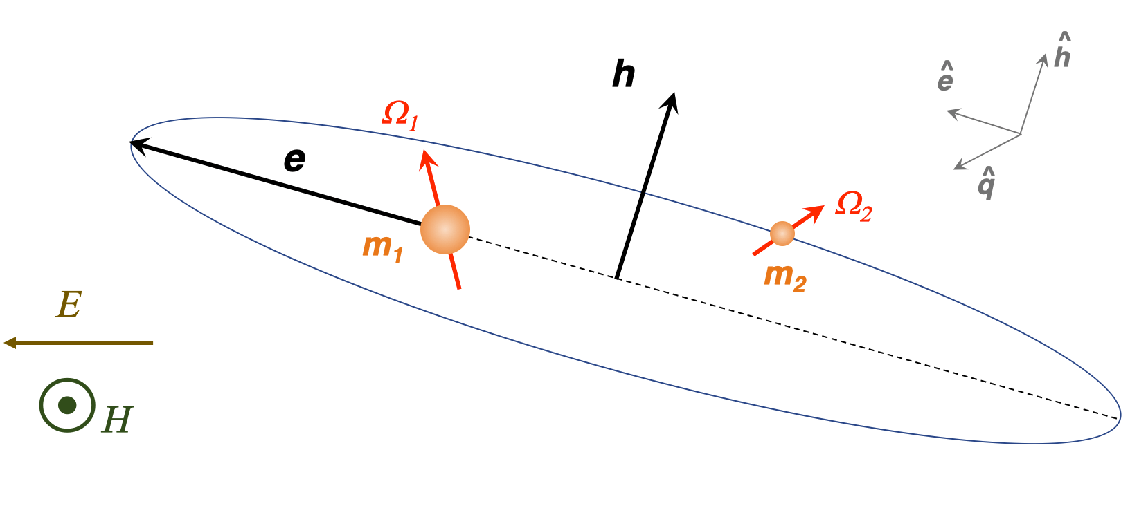
Figure 1.— Orientation of the vectors for the Kozai cycles plus tidal friction model. The model solves for the eccentricity vector ${\boldsymbol{e}}$, the angular momentum ${\boldsymbol{h}}$ of the inner binary, and the spin angular momentum of each body, ${\boldsymbol{\Omega}}_{1}$ and ${\boldsymbol{\Omega}}_{2}$. The vectors ${\boldsymbol{e}}$, ${\boldsymbol{h}}$, and ${\boldsymbol{q}}={\boldsymbol{h}}\times{\boldsymbol{e}}$ define a system of time-varying orthogonal bases. The eccentricity and angular momentum vectors of the outer orbit, ${\boldsymbol{E}}$, and ${\boldsymbol{H}}$, remain constant. The orbital inclination is the angle between ${\boldsymbol{h}}$ and ${\boldsymbol{H}}$.

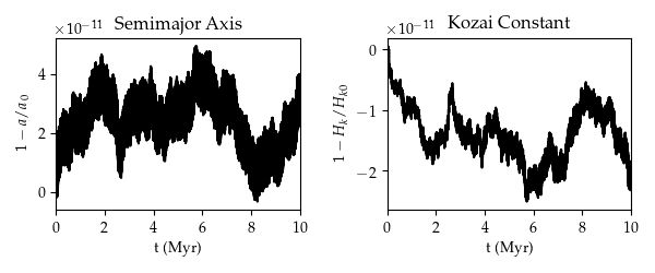
Figure 2.— Conservation of the semimajor axis and of the Kozai constant $H_{k}=\cos{I}\sqrt{1-e^{2}}$ related to the vertical angular momentum. With an adaptative timestep responding to period and eccentricity, we achieve conservation down to $10^{-11}$ over 10 Myr.

In this work we use two different codes. The first is a $N$-body model that solves for position and velocities of point masses under mutual gravitational interaction. The second is a Kozai cycle plus tidal friction model, which evolves the eccentricity vector and the orbital angular momentum of the binary, along with the spin angular momenta of the two bodies, while keeping the external, heliocentric, orbit constant (see 1). Both use a standard 3rd order Runge-Kutta, i.e., the accumulated error is proportional to the cube of the timestep.

2.1. The KTJD model

We follow the equations of Eggleton & Kiseleva-Eggleton (2001) in the reference frame of the orbit of the binary. The (time-varying) orientation is given by the unit vectors $\hat{{\boldsymbol{e}}}$ pointing to pericenter, $\hat{{\boldsymbol{h}}}$ pointing to the direction of orbital angular momentum, and $\hat{{\boldsymbol{q}}}=\hat{{\boldsymbol{h}}}\times\hat{{\boldsymbol{e}}}$ along the latus rectum (see 1).

We split the model equations for the eccentricity and angular momentum vectors into equations for their moduli and unit vectors, respectively. The full model including the evolution of the spin vectors consists of 14 coupled equations

$$\frac{de}{dt} = -e\left[V_{1}+V_{2}+V_{d}+5\left(1-e^{2}\right)S_{eq}\right],$$ (1)

$$\frac{dh}{dt} = -h\left(W_{1}+W_{2}+W_{d}-5e^{2}S_{eq}\right),$$ (2)

$$\frac{d\hat{{\boldsymbol{e}}}}{dt} = \left[Z_{1}+Z_{2}+\left(1-e^{2}\right)\left(4S_{ee}-S_{qq}\right)\right]\hat{{\boldsymbol{q}}}$$ (3)

$$- \left[Y_{1}+Y_{2}+\left(1-e^{2}\right)S_{qh}\right]\hat{{\boldsymbol{h}}},$$

$$\frac{d\hat{{\boldsymbol{h}}}}{dt} = \left[Y_{1}+Y_{2}+\left(1-e^{2}\right)S_{qh}\right]\hat{{\boldsymbol{e}}}$$ (4)

$$- \left[X_{1}+X_{2}+\left(4e^{2}+1\right)S_{eh}\right]\hat{{\boldsymbol{q}}},$$

$$\frac{d{\boldsymbol{\Omega}}_{1}}{dt} = \frac{\mu_{r}h}{\mathcal{I}_{1}}\left(-Y_{1}\hat{{\boldsymbol{e}}}+X_{1}\hat{{\boldsymbol{q}}}+W_{1}\hat{{\boldsymbol{h}}}\right),$$ (5)

$$\frac{d{\boldsymbol{\Omega}}_{2}}{dt} = \frac{\mu_{r}h}{\mathcal{I}_{2}}\left(-Y_{2}\hat{{\boldsymbol{e}}}+X_{2}\hat{{\boldsymbol{q}}}+W_{2}\hat{{\boldsymbol{h}}}\right).$$ (6)

Here the indices 1 and 2 refer to each orbiter of the inner binary. The quantities $V_{i}$ and $W_{i}$ ($i=1,2$) are dissipative functions related to how a deformable body responds to a tidal field. The quantities $X$, $Y$, $Z$ give precession and apsidal motion. The tensor $S_{ij}$ relates to the 3rd body and is responsible for the Kozai cycles, here added up to the quadrupole level of approximation (Kiseleva et al., 1998) and keeping the outer orbit exactly constant ($a_{\rm out}=45$ AU and $e_{\rm out}=0.04$ for MU69). In the model, the outer orbit is specified by the time-independent vectors ${\boldsymbol{H}}$ and ${\boldsymbol{E}}$, the angular momentum and eccentricity vectors of the outer orbit, respectively.

We refer the reader to Eggleton & Kiseleva-Eggleton (2001) for the detailed mathematical form of the parameters $X$, $Y$, $Z$, $V$, $W$, and $S_{ij}$, and to Ragozzine (2009) to how the planetary permanent quadrupole impacts these parameters, depending also on the rigidity $\mu_{\rm b}$ of the body and the tidal dissipation quality factor $Q$. The parameter $\mathcal{I}_{i}=0.4m_{i}(R_{xi}^{2}+R_{yi}^{2})$ is the moment of inertia of body $i$ about its spin axis, and we do not consider non-principal axis rotators; $m_{i}$ is the mass of body $i$; $R_{xi}$ and $R_{yi}$ are the principal semiaxes of body $i$ perpendicular to the spin axis. Finally, $\mu_{r}=m_{1}m_{2}/(m_{1}+m_{2})$ is the reduced mass.

The integration timestep is adaptive with semimajor axis and eccentricity,

$$\Delta t=CT\sqrt{\frac{1-e}{1+e}}$$ (7)

where $T$ is the orbital period of the inner binary, updated as it hardens. The factor in the square root is the velocity at pericenter normalized by the circular velocity. We find this important to conserve energy and angular momentum during the high-eccentricity excursions. We test a non-dissipative, purely Kozai cycle model, to 10 Myr, and find that with $C=10^{-2}$ the semimajor axis and the Kozai constant are conserved and bounded to one part in $10^{11}$ (2). We test that decreasing $C$ to $10^{-3}$ does not improve conservation, and for $C=10^{-1}$ the error grows. We use thus $C=10^{-2}$ in all integrations. The code, written in Fortran90, is made public and can be downloaded from https://github.com/wlyra/yoshikozai

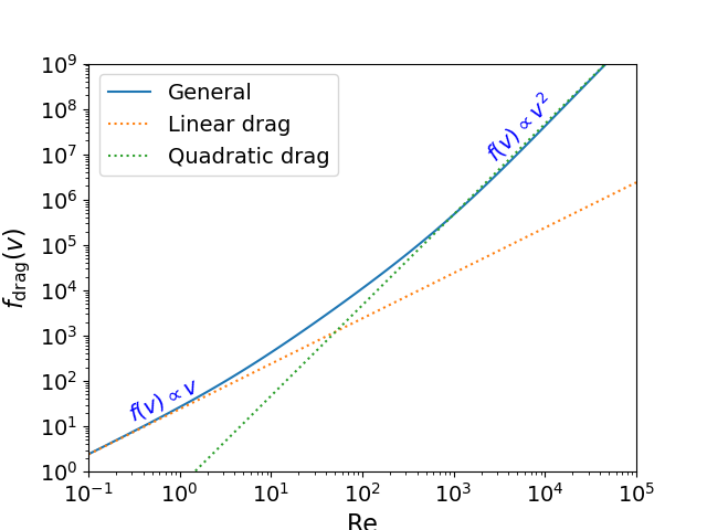
Figure 3.— Dependency of the drag regime ($F_{\rm drag}\propto C_{D}\mathrm{Re}^{2}$) on Reynolds number. The drag is linear in the viscous regime (Stokes law) and quadratic in the turbulent (ram pressure) regime, with a smooth transition in between. MU69 in the MMSN lies at $\mathrm{Re}\approx 10$, closer to the linear range.

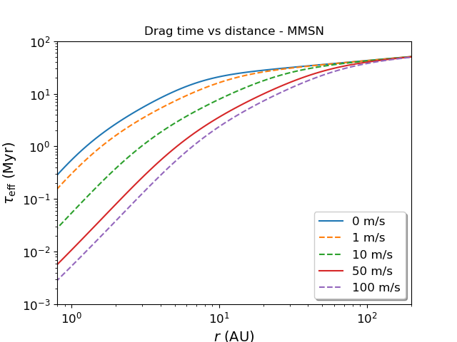
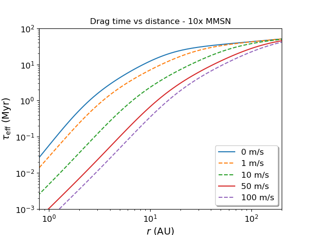
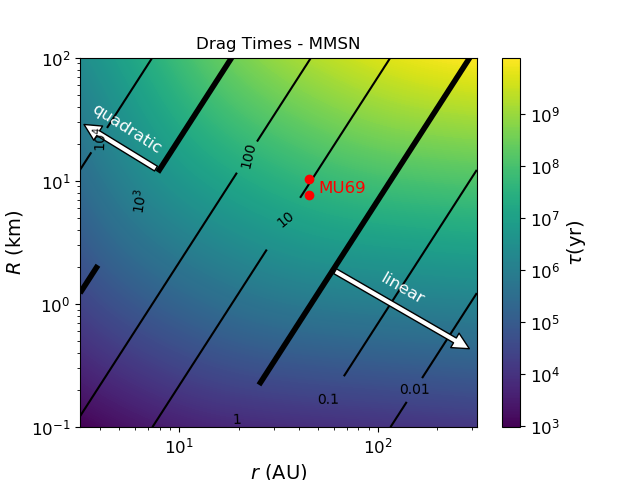
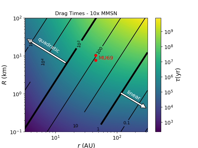
Figure 4.— Upper panels: Effective drag time vs distance for bodies the size and mass of MU69 as function of the wind velocity in the MMSN (left) and a solar nebula ten times more massive (right). The red curve (50 m/s) corresponds to standard pressure gradients, zero (blue) to a local pressure maximum, and others speeds to reduced or enhanced pressure gradients. For the no-wind curve (blue) only the binary velocity is considered. Stokes drag, where the wind has no effect, is valid in the Kuiper belt. In the asteroid belt the Reynolds number place the drag force in the quadratic regime, and the wind brings the effective drag time down to 0.1 Myr. Nebular drag can collapse an object like MU69 in the asteroid belt in the lifetime of the Solar Nebula, but not in the Kuiper belt. Lower panels: Drag times as a function of distance (x-axis) and body radius (y-axis) in the MMSN (left) and a solar nebular ten times more massive (right), assuming a 50 m/s wind. The color maps refers to drag times. The lines to Reynolds numbers. MU69 lies in the transition between linear drag (${\rm Re}<1$) and quadratic drag (${\rm Re}>1000$).

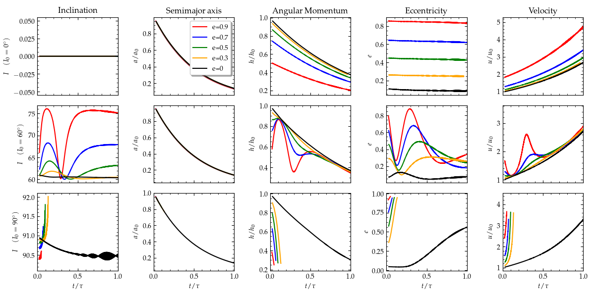
Figure 5.— $N$-body evolution of a binary of initial inclination $0^{\circ}$ (top panels), $60^{\circ}$ (middle panels) and $90^{\circ}$ (bottom panels) for a range of initial eccentricities. The lines are box-averaged over a solar period. Time is normalized by the friction time $\tau$. The long-term evolution in zero inclination is well described by the analytical solution for $a$,$e$, $h$ averaged over a solar orbit. The system comes to contact within the timescale set by $\tau$. This is appropriate for contact within the lifetime of the Solar nebula for the range of semimajor axes of the asteroid belt ($\tau_{\rm eff}\approx 0.1$ Myr), but would not lead to contact in the Kuiper Belt ($\tau_{\rm eff}>10$ Myr). For $I_{0}=60^{\circ}$ one Kozai cycle is seen to occur. Yet, the eccentricity does not rise high enough to lead to contact. For $I_{0}=90^{\circ}$ initial inclination rapid evolution to contact happens, even for moderately low eccentricities ($e\gtrsim 0.3$). The evolution is of very fast fall of angular momentum and increase of eccentricity with nearly constant semimajor axis, plunging the binary into contact through a nearly radial trajectory.

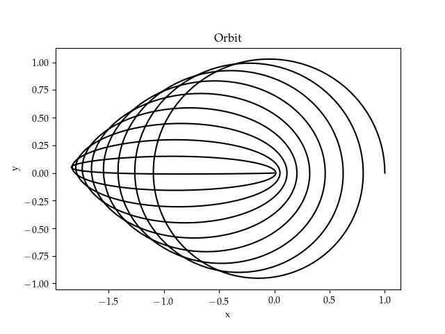
Figure 6.— The trajectory to contact in the reference frame of the primary of the inner binary, oriented along the $\hat{{\boldsymbol{e}}}\hat{{\boldsymbol{q}}}\hat{{\boldsymbol{h}}}$ vectors, here fixed. The secondary started at ($x,y$)=(1,0) and ended at the origin. Its trajectory was one of flattening the $y$ axis while the magnitude of the semimajor axis remains roughly constant, increasing the eccentricity and losing angular momentum.

Table 1Symbols used in this work.

Symbol	Definition	Description		Symbol	Definition	Description
$a$		semimajor axis of inner binary		$\Delta{\boldsymbol{v}}$	${\boldsymbol{v}}-{\boldsymbol{u}}$	velocity of flow past object
$a_{\rm out}$		semimajor axis of outer binary		$d{\boldsymbol{F}}$		force differential
$h$		inner binary angular momentum		$\hat{{\boldsymbol{r}}}$		cylindrical rotation of $\hat{{\boldsymbol{e}}}$
$h_{\rm out}$		outer binary angular momentum		$\hat{{\boldsymbol{\phi}}}$		cylindrical rotation of $\hat{{\boldsymbol{q}}}$
$H$	$h+h_{\rm out}$	total angular momentum		$\overline{R}$	$d{\boldsymbol{F}}\cdot\hat{{\boldsymbol{r}}}$	radial force
$t$		time		$\overline{T}$	$d{\boldsymbol{F}}\cdot\hat{{\boldsymbol{\phi}}}$	azimuthal force
$I$	$\cos^{-1}(h_{z}/h)$	mutual inclination of inner binary		$\overline{N}$	$d{\boldsymbol{F}}\cdot\hat{{\boldsymbol{h}}}$	vertical force
$e$		eccentricity of inner binary		$f$		true anomaly
$H_{k}$	$\cos I\sqrt{1-e^{2}}$	Kozai constant		$E$	$M=E-e\sin E$	eccentric anomaly
$\omega$		longitude of pericenter		$M$	$nt$	mean anomaly
$m_{1}$		mass of primary		$\boldsymbol{\mathrm{R}}$		Rotation matrix
$m_{2}$		mass of secondary		$m_{b}$	$m_{1}+m_{2}$	sum of masses of bodies
$M_{\odot}$		solar mass		$R_{b}$	$R_{1}+R_{2}$	sum of radii of bodies
$R_{H}$	$a\left(\frac{m_{1}+m_{2}}{3M_{\odot}}\right)^{1/3}$	Hill radius		$\mu$	$Gm_{b}$
$\hat{{\boldsymbol{e}}}$	${\boldsymbol{e}}/e$	unit eccentricity vector		$\varOmega$		longitude of ascending node
$\hat{{\boldsymbol{h}}}$	${\boldsymbol{h}}/h$	unit angular momentum vector		$\rm T$		temperature
$\hat{{\boldsymbol{q}}}$	$\hat{{\boldsymbol{h}}}\times\hat{{\boldsymbol{e}}}$			$\lambda_{\rm mfp}$	$\frac{\mu_{\rm mol}\ m_{H}}{\rho\sigma_{\rm coll}}$	mean free path
${\boldsymbol{\Omega}}_{1}$		spin of primary		$T_{\rm out}$	$2\pi/n_{\rm out}$	period of outer binary
${\boldsymbol{\Omega}}_{2}$		spin of secondary		$\mu_{\rm mol}$		mean molecular weight
$\mu_{r}$	$\frac{m_{1}m_{2}}{m_{1}+m_{2}}$	reduced mass		$m_{H}$		atomic mass unit
$\mathcal{I}_{1}$	$\frac{2}{5}m_{1}\left(R_{x1}^{2}+R_{y1}^{2}\right)$	inertia moment of primary		$\sigma_{\rm coll}$		collisional cross section
$\mathcal{I}_{2}$	$\frac{2}{5}m_{2}\left(R_{x2}^{2}+R_{y2}^{2}\right)$	inertia moment of secondary		$\mu_{\rm visc}$		dynamical viscosity
$T$	$2\pi/n$	period of inner binary		$c_{s}$		sound speed
$R_{x}$		principal semiaxis of ellipsoid		$P$	$\rho c_{s}^{2}$	pressure
$R_{y}$		principal semiaxis of ellipsoid		$\Sigma$	$\int\rho dz$	column density
$R_{z}$		principal semiaxis of ellipsoid		$p$		power law of column density
$R$	$(R_{x}R_{y}R_{z})^{1/3}$	equivalent radius of ellipsoid		$\rm Ma$	$|\Delta v|/c_{s}$	Mach number
$J_{2}$	$\frac{1}{10}\frac{R_{x}^{2}+R_{y}^{2}-2R_{z}^{2}}{R^{2}}$	quadrupole potential		$\rm Kn$	$\frac{\lambda_{\rm mfp}}{2R}$	Knudsen number
$\tau_{1}$	$\frac{8}{3C_{D}}\frac{R_{1}}{|\Delta{\boldsymbol{v}}|}\frac{\rho_{\bullet}}{\rho}$	drag time of the primary		$\tau_{w}$	$\frac{\tau_{1}\tau_{2}}{\tau_{1}-\tau_{2}}$	wind drag timescale
$\tau_{2}$	$\frac{8}{3C_{D}}\frac{R_{2}}{|\Delta{\boldsymbol{v}}|}\frac{\rho_{\bullet}}{\rho}$	drag time of the secondary		$\tau_{m}$	$\tau_{\rm eff}$	orbital drag timescale
$\tau_{\rm eff}$	$\frac{\tau_{1}\tau_{2}(m_{1}+m_{2})}{\tau_{2}m_{2}+\tau_{1}m_{1}}$	effective drag time of binary		$e_{\rm out}$	$|{\boldsymbol{E}}|$	eccentricity of outer binary
$\rho_{\bullet}$		internal density		${\boldsymbol{x}}$	$x\hat{{\boldsymbol{x}}}+y\hat{{\boldsymbol{y}}}+z\hat{{\boldsymbol{z}}}$	local Hill coordinates
$G$		gravitational constant		${\boldsymbol{x}}_{\rm cart}$	$x_{c}\hat{{\boldsymbol{e}}}+y_{c}\hat{{\boldsymbol{q}}}+z_{c}\hat{{\boldsymbol{h}}}$	Cartesian coords. on orbital frame
$n_{\rm out}$	$\sqrt{\frac{GM_{\odot}}{a_{\rm out}^{3}}}$	mean motion of outer binary		${\boldsymbol{x}}_{\rm cyl}$	$\boldsymbol{\mathrm{R}}_{h}(-f){\boldsymbol{x}}_{\rm cart}$	Cylindrical coords. on orbital frame
$v_{\rm out}$	$n_{\rm out}a_{\rm out}$	circular velocity of outer binary		${\boldsymbol{E}}$		eccentricity vector of outer orbit
$a_{1}$	$\frac{m_{2}}{m_{1}+m_{2}}a$	semimajor axis of primary		$Q$		tidal dissipation factor
$a_{2}$	$\frac{m_{1}}{m_{1}+m_{2}}a$	semimajor of secondary		${\boldsymbol{s}}_{1}$		distance origin-primary
$v_{1}$	$na_{1}$	circular velocity of primary		${\boldsymbol{s}}_{2}$		distance origin-secondary
$v_{2}$	$na_{2}$	circular velocity of secondary		${\boldsymbol{r}}_{1}$	$-\frac{m_{2}}{m_{1}+m_{2}}{\boldsymbol{r}}$	distance barycenter-primary
$\eta$		sub-Keplerian parameter		${\boldsymbol{r}}_{2}$	$\frac{m_{1}}{m_{1}+m_{2}}{\boldsymbol{r}}$	distance barycenter-secondary
$u$	$\eta v_{\rm out}$	wind velocity		$s_{\rm cm}$		distance barycenter-origin
$u_{\rm eff}$	$u\frac{(\tau_{2}-\tau_{1})(m_{1}+m_{2})}{(m_{2}\tau_{2}+m_{1}\tau_{1})}$	effective wind		$M_{\rm out}$	$n_{\rm out}t$	mean anomaly of outer orbit
$\rho$		gas density		$t_{\rm kozai}$	Eq. (30)	timescale of Kozai-Lidov cycle
$C_{D}$	Eq. (23)	drag coefficient		$f_{H}$	$a/R_{H}$	semimajor axis in Hill radii
$\mathrm{Re}$	$2R\rho|\Delta{\boldsymbol{v}}|/\mu_{\rm visc}$	Reynolds number past the object		$b_{c}$		impact parameter
$n$	$\sqrt{\frac{Gm_{b}}{a^{3}}}$	mean motion of inner binary		$f_{D}$	$b_{c}/\bar{D}$	impact parameter in binary diameters
$v_{\rm esc}$	$\sqrt{2G(m_{1}+m_{2})/R}$	escape velocity		$\nu$	$\frac{16}{3}\frac{n}{n_{\rm out}}$	normalized ratio of mean motions
$q$	$a(1-e)$	pericenter distance		$\beta$	$\frac{16}{3\nu^{2}}$	normalized ratio of mean motions
$\mu_{\rm b}$		rigidity		$M_{\beta}$	$\beta M$	scaled mean anomaly
${\boldsymbol{r}}$		separation of inner binary		$\Psi$	$\Omega-\nu M_{\beta}$	modified longitude of ascending node
$\bar{D}$	$\left(\frac{8}{\pi}\frac{m_{1}+m_{2}}{\rho_{\bullet}}\right)^{1/3}$	effective combined diameter

2.2. Nebular Drag

Gas drag enters the equations as the dissipation parameters $V_{d}$ and $W_{d}$ in eccentricity and angular momentum, respectively. Notice that while $W_{i}$ are related to spin-orbit coupling, with the orbit and spin angular momenta equations having equal and opposite terms, $W_{d}$ has no such symmetry. This is because the angular momentum taken from the orbital motion by the drag is not conserved by converting it into rotational angular momentum, but given to the nebular gas.

To find the values of $V_{d}$ and $W_{d}$, we work out the orbital solution in the presence of drag, which is shown in detail in appendix A. The solution, despite a lengthy and laborious derivation, turns out to be remarkably simple. If $a_{0}$, $e_{0}$, and $h_{0}$ are the initial semimajor axis, eccentricity and angular momentum of the inner binary, the solution at a time $t$ is given by

$$\tilde{a} = a_{0}\mathrm{e}^{-2t/\tau_{\rm eff}}$$ (8)

$$\tilde{e} = e_{0}$$ (9)

$$\tilde{h} = h_{0}\mathrm{e}^{-t/\tau_{\rm eff}}$$ (10)

where tilde represents average over the solar orbit, and

$$\tau_{\rm eff}=\frac{\tau_{1}\tau_{2}(m_{1}+m_{2})}{\tau_{2}m_{2}+\tau_{1}m_{1}}$$ (11)

is the effective drag time. Here $\tau_{1}$ and $\tau_{2}$ are the drag times on the primary and secondary, respectively. The eccentricity is constant, while the angular momentum decays exponentially in an e-folding time equal to the effective drag time. As consequence, the energy decays at twice the rate of the angular momentum. Equations Eq. (9) and Eq. (10) lead to the coefficients

$$V_{d} = 0,$$ (12)

$$W_{d} = -\frac{1}{\tau_{\rm eff}}.$$ (13)

2.3. Parameters of MU69

We consider that MU69 was a binary system that came into contact, the lobes being the primary and secondary masses $m_{1}$ and $m_{2}$. The dimensions of the lobes denote a volume ratio of roughly 2:1. The equivalent radius of spheres of same volume are $R_{1}=7.8$ km and $R_{2}=6.4$ km. The parameter $J_{2}$ for each lobe, assuming a homogeneous triaxial ellipsoid (Scheeres, 1994), is given by

$$J_{2}=\frac{1}{10}\frac{\left(R_{x}^{2}+R_{y}^{2}-2R_{z}^{2}\right)}{R^{2}}$$ (14)

where $R_{x}$, $R_{y}$, and $R_{z}$ are the principal semi-axes. For the lobes of MU69, the observed values of $R_{x}$ ,$R_{y}$, and $R_{z}$ lead to $J_{2}$ = 0.26 and 0.14 ($\pm 0.07$) for the larger and smaller lobes, respectively. Assuming an internal density of $\rho_{\bullet}$ = 0.5 g/cm³, the masses are $m_{1}=1.01\times 10^{18}$g and $m_{2}=5.45\times 10^{17}$ g. At the distance of $a_{\rm out}=$45 AU, the center of mass orbits the Sun at the velocity of $v_{\rm out}=n_{\rm out}a_{\rm out}\approx$ 4.5 km/s, where $n_{\rm out}$ is the mean motion of the heliocentric orbit. The Hill radius of the combined masses is $R_{H}=a_{\rm out}[m_{b}/(3M_{\odot})]^{1/3}$, where $m_{b}=m_{1}+m_{2}$ is the sum of the masses of the primary and secondary and $M_{\odot}$ is the solar mass. Substituting the masses obatined above yields $R_{H}\approx 2.8\times 10^{-4}$ AU, or $4.3\times 10^{4}$ km.

For a representative semimajor axis $a=0.1R_{H}\approx 4300\ {\rm km}$ the period is $T=5.6\,{\rm yr}$. The semimajor axes of the orbits around the barycenter and respective circular orbital velocities are $a_{2}=2785\,{\rm km}$, $a_{1}=1505\,{\rm km}$, and $v_{2}=10\,{\rm cm\,s^{-1}}$, $v_{1}=5.5\,{\rm cm\,s^{-1}}$.

These orbital velocities are very small. The velocity of the center of mass around the Sun, $v_{\rm out}=4.5$ km/s, is over $40\,000$ times larger. For the minimum-mass Solar nebula (MMSN, Weidenschilling, 1977; Hayashi, 1981) at 45 AU, the gas is sub-Keplerian by $n_{\rm gas}=n_{\rm out}(1-\eta)$, where $n_{\rm out}$ is the Keplerian value and $\eta\sim 0.01$. The wind that the binary is experiencing is then

$$u=\eta v_{\rm out}\approx 50\,{\rm m\,s^{-1}}.$$ (15)

i.e., about 500 times faster than the circular velocity of the binary. The sub-Keplerian wind cannot in principle be ignored. We find in appendix A that in the reference frame of motion around the primary, the effective wind is

$${\boldsymbol{u}}_{\rm eff}={\boldsymbol{u}}\frac{(\tau_{2}-\tau_{1})(m_{1}+m_{2})}{(m_{2}\tau_{2}+m_{1}\tau_{1})}.$$ (16)

The model is fully specified if the drag times are known. These are considered in the next section.

2.3.1 Drag time

Solid particles and gas exchange momentum due to interactions that happen at the surface of the solid body. The many processes that can occur are generally described by the collective name of “drag” or “friction”. Consider a solid body of cross section $\sigma$ travelling through a fluid medium of uniform density $\rho$ with velocity ${\boldsymbol{v}}$ with respect to the fluid. In a time interval $dt$, it sweeps a volume $dV=\sigma vdt$. In the reference frame of the particle, the gas molecules are travelling with velocity $-{\boldsymbol{v}}$. If all their momentum is transferred to the particle, the force is

$$F_{\rm drag}=\rho dV\frac{d{\boldsymbol{v}}}{dt}=-\rho\sigma v{\boldsymbol{v}}.$$ (17)

In aerodynamics it is usual to define a dimensionless factor $C_{D}$ that takes into account the deviations from this idealized picture

$$F_{\rm drag}=-\frac{1}{2}C_{D}\rho\sigma v{\boldsymbol{v}}.$$ (18)

The factor half comes in because it is common to define the drag force in terms of kinetic energy instead of momentum. Considering spheres of radius $R$, their cross section is $\sigma=\pi R^{2}$; the acceleration $f_{\rm drag}$ in the equation of motion is found upon dividing $F_{\rm drag}$ by the mass of the object $m=4\pi R^{3}\rho_{\bullet}/3$, where $\rho_{\bullet}$ is the material density

$$f_{\rm drag}=-\left(\frac{3\rho C_{D}v}{8R\rho_{\bullet}}\right){\boldsymbol{v}}.$$ (19)

The quantity in parentheses has dimension of time^-1, defining the drag time of an embedded object

$$\tau\equiv\frac{8}{3C_{D}}\frac{R}{v}\frac{\rho_{\bullet}}{\rho}.$$ (20)

The drag time represents the timescale within which the object couples to the gas flow. The parameter $C_{D}$ can be calculated from first principles or derived from experiments, depending on the drag regime of interest. When the object radius exceeds the mean free path of the particle, the approximation of ballistic collisions ceases to apply and the frequent intermolecular collisions lead to the emergence of viscous behaviour. It is a well-known result that ideal fluids exert no drag (d’Alembert’s paradox). When the kinematic viscosity $\mu_{\rm visc}$ is considered, Stokes drag law on a large sphere (large meaning bigger than the mean free path of the gas) is recovered

$$F_{\rm drag}^{\rm(Stk)}=-6\pi\mu_{\rm visc}R{\boldsymbol{v}},$$ (21)

a lengthy proof of which can be found in Landau & Lifshitz (1987). Dividing Eq. (21) by the mass of the object and expressing it in the form of Eq. (18), one finds

$$C_{D}^{\rm(Stk)}=\frac{12\mu_{\rm visc}}{R\rho v}=\frac{24}{\mathrm{Re}}$$ (22)

On obtaining this equation, the inertia of the fluid is neglected, so it only holds for low Reynolds numbers. Empirical corrections to Stokes’ law were worked out (e.g., Arnold 1911, Millikan 1911, Millikan 1923), but a general case derived from first principles is difficult to obtain. The major complication resides at the boundary layer immediately over the surface of the particle, where the velocity of the viscous fluid has to be zero. If the fluid has inertia, a sharp velocity gradient develops in the flow past the object as the velocity goes to zero at the solid surface. At this boundary layer, the viscous term is important even at high Reynolds numbers (Prandtl 1905). It can be seen experimentally that in such cases, the flow past the particle develops into a turbulent wake (von Karman 1905), with drag coefficients much larger than those predicted by Stokes law.

Experiments with hard spheres (Cheng, 2009) show that the drag coefficient $C_{D}$ for large objects and valid in the range $\mathrm{Re}<2\times 10^{5}$ can be fit by the following empirical formula (Perets & Murray-Clay, 2011)

$$C_{D}=\frac{24}{\mathrm{Re}}\left(1+0.27\right)^{0.43}+0.47\left[1-\exp{(-0.04\mathrm{Re}^{0.38})}\right].$$ (23)

The value of $C_{D}$ varies non-monotonically, being $C_{D}\approx 26$ for $\mathrm{Re}=1$, reaching a minimum of $C_{D}\approx 0.25$ at $\mathrm{Re}=10^{3}$ and rising to $C_{D}\approx 0.45$ at $\mathrm{Re}=10^{5}$. The drag times for the pre-merger lobes of MU69 are $\tau_{1}=2.87\times 10^{7}$ yr and $\tau_{2}=2.00\times 10^{7}$ yr (details of the calculation are shown in appendix  B). The system can thus be modeled as going through an effective headwind $u_{\rm eff}=166\,u\approx 25$ m/s with effective friction time $\tau_{\rm eff}=2.24\times 10^{7}$ yr.

We highlight that because $F_{\rm drag}\propto C_{D}\mathrm{Re}^{2}$, in the low Reynolds number regime, with $C_{D}$ given by Eq. (22), the drag force is linear with velocity ($\mathrm{Re}\propto v$). Conversely, in the regime of high Reynolds number ($\mathrm{Re}\approx 10^{3})$, $C_{D}$ asymptotes to a constant value, and Eq. (18) becomes quadratic with velocity. This is the regime of turbulent, or ram pressure, drag. The different regimes are shown in the left panel of 3, where the y-axis is $C_{D}\mathrm{Re}^{2}$. As seen in the figure, linear drag is valid up to $\mathrm{Re}\approx 1$, and quadratic beyond $\mathrm{Re}\approx 1000$ with a smooth transition in between. For MU69 at 45 AU in the MMSN, the Reynolds number is $\mathrm{Re}\approx 10$, placing it much closer to linear (viscous) than to quadratic (turbulent) drag. This distinction has profound consequences for the orbital evolution of the pre-merger lobes of MU69.

3. Results

3.1. Inability of drag alone to lead to contact in the Kuiper belt

The drag times for bodies of the size of MU69 as a function of distance are shown in the upper panels of 4. In these curves the Reynolds number is calculated by having the velocity being the sum of the wind and the orbital velocity (at a representative distance of 0.1 $R_{H}$ from the central object with mass equal to the combined mass of MU69). The left panel is the MMSN, and the right panel a solar nebula ten times more massive than the MMSN. The different lines are different values for the wind velocity. The red solid line corresponds to standard pressure gradients, yielding wind velocities of $\approx$ 50 m/s. The blue solid line is no wind, corresponding to a pressure maximum. The other lines represent reduced or enhanced pressure gradients, for comparison.

In the outer disk the Reynolds number is low enough that viscous linear drag ensues and the presence of the wind does not matter. This is because if the drag is linear, the angular momentum gained in half an orbit is exactly lost in the other half whereas for quadratic drag the influence of the wind does not cancel out exactly when averaged over an orbit (cf. Sect 3.2 of Perets & Murray-Clay, 2011); as a result, in the inner disk where the drag is quadratic, the influence of the wind in the drag time is dominant. The upper panels of 4 shows that the wind-enhanced orbital drag alone, with no Kozai cycles, is able to collapse a MU69-like binary in the asteroid belt in the timeframe of the lifetime of the disk, but not in the Kuiper belt, either in the MMSN or in a nebular ten times more massive.

The lower panels of 4 show drag time (color coded) and Reynolds numbers (solid lines) as a function of distance in AU and body radius in km, for a wind speed of 50 m/s. The regimes of linear (Re $<$ 1) and quadratic drag (Re $>$ 10³) are shown as thicker solid lines and arrows. The pre-merger lobes of MU69 are shown as red dots in both plots: as seen in the figures, they lie in the transition between linear and quadratic drag. In the MMSN the Reynolds number is about 10, closer to linear, with drag times of $\approx$20 Myr; for the more massive model (10x MMSN) the Reynolds number is closer to 100. In this more massive case the drag time is $\approx$10 Myr; the effect of the wind, even though closer to quadratic than to linear, is still not enough to lower the drag time to values within the lifetime of the nebula.

For the Kuiper belt, the timescales of the problem are, in decreasing order: dynamical ($n$, where $n$ is the orbital mean motion); Coriolis force ($n_{\rm out}\approx 10^{-2}n$); centrifugal ($n_{\rm out}^{2}\approx 10^{-4}n$); wind $(u/\tau\approx 10^{-5}n)$; orbital drag ($1/\tau\approx 10^{-7}n$); shear ($n_{\rm out}/\tau\approx 10^{-9}n$). We plot in 5 the $N$-body evolution of a binary of point masses, subject to gas drag, with initial inclination $I$=0^∘, 60^∘, and 90^∘, for a range of eccentricities. The lines shown are box-averages over a solar period.

The zero inclination curves show the predicted behavior of semimajor axis, eccentricity and angular momentum, averaged over a solar orbit. The system has an exponential decay of angular momentum and semimajor axis, with e-folding time defined by the drag time $\tau$. This rate of decay is enough to lead to collapse in the asteroid belt, where the quadratic drag aided by the wind brings $\tau$ to 0.1 Myr timescales. Yet, at the Kuiper belt, as discussed above, the timescales remain of the order of 10 Myr, hindering collapse.

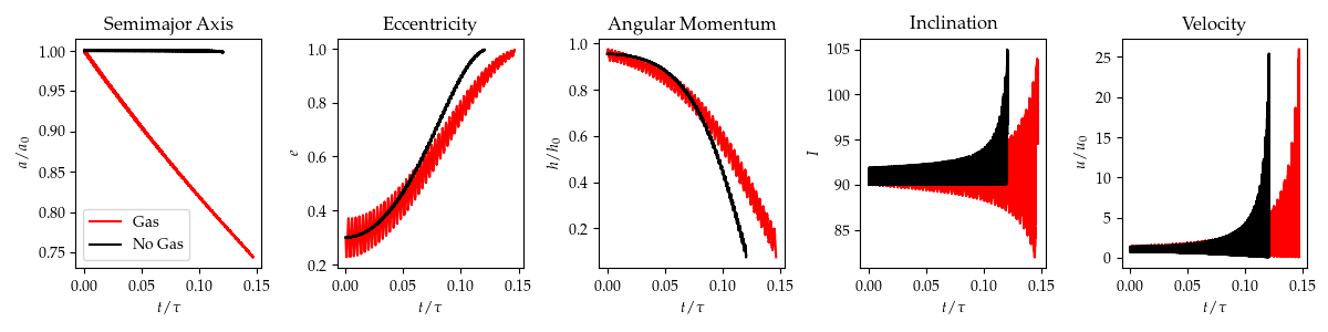
Figure 7.— Comparison between the model shown for $90^{\circ}$ on 5 and the same model but switching off nebular drag. The evolution is mainly driven by the Kozai oscillations, with gas playing a secondary role and the wind driving the eccentricity and angular momentum oscillation. Notice how nebular drag makes the inclination flip between prograde and retrograde, and how the velocity increases to 20-25 times the initial orbital velocity as the eccentricity approaches unity.

3.2. Kozai-driven collapse in the Kuiper belt

The $I=60^{\circ}$ plots show oscillations of eccentricity and inclination; we measure that these oscillations conserve the Kozai constant $H_{k}$, characterizing Kozai-Lidov oscillations. Still the excursions into high eccentricity are not enough to make the orbit grazing (separation less than 30 km) even for initial eccentricity $e_{0}=0.9$ over 10 Myr.

The situation changes for $I=90^{\circ}$. Now, for moderate initial eccentricities, the eccentricity shoots to unity in very short timescales, and the orbit becomes grazing, reaching separation $r=30$ km in timescales of the order of $0.1\tau$. The collapse happens essentially at constant energy. The orbit is forced from initially circular into a progressively elongated ellipse and finally into a straight line, leading to contact (6).

Since the orbit is Keplerian, we can analytically calculate the velocity at contact. For a head-on collision at pericenter

$$v=\sqrt{\frac{G(m_{1}+m_{2})}{a}\left(\frac{1+e}{1-e}\right)}$$ (24)

where $G$ is the gravitational constant. Writing $v_{\rm esc}=\sqrt{2G(m_{1}+m_{2})/R}$ for the escape velocity ($R$ being the effective radius of MU69), we can write this equation as

$$\frac{v}{v_{\rm esc}}=\sqrt{\frac{R}{q}\left(1-\frac{q}{2a}\right)}$$ (25)

where $q$ is the pericenter distance. If contact happens along the principal axes, $q=(R_{x1}+R_{x2})/2\ll a$ (the subscripts 1 and 2 refer to primary and secondary bodies), and we have

$$\frac{v}{v_{\rm esc}}=\frac{(R_{x1}R_{y1}R_{z1}+R_{x2}R_{y2}R_{z2})^{1/6}}{(R_{x1}+R_{x2})^{1/2}}.$$ (26)

For the parameters of MU69, this yields $v\approx 0.71v_{\rm esc}$, i.e. about 70% reduction compared to the escape velocity. The escape velocity depends on the bulk density of MU69, which is not well constrained. The velocity at contact is

$$v\approx 4.2\,{\rm m\,s^{-1}}\ \sqrt{\frac{\rho_{\bullet}}{0.5\,{\rm g\,cm^{-3}}}}.$$ (27)

An internal density of 0.3 g cm^-3 leads to contact at velocity 3.3 m s^-1. Collision velocities in the range $2-3$ m s^-1 happen for internal densities in the range $0.12-0.25$ g cm^-3. 7 shows a comparison of the same simulation with nebular drag switched on and off. Gas drag plays a secondary role: the evolution is driven mostly by Kozai-Lidov cycles. Just how secondary the role of nebular drag is is explored in the next section with our Kozai-Tides-J2-drag model.

3.3. Gas-enhanced Kozai

The orbital integrations shown in 5 treat the bodies as point masses, which are gravitational monopoles and impervious to tides. To relax this approximation, we make use of the orbit-integrated KTJD model described in Sect. 2. For the tidal model we use rigidity $\mu_{\rm b}=4\times{10^{10}}$ g cm^-1 s^-2 and tidal dissipation quality $Q=100$, as typically assumed for icy bodies (Ragozzine & Brown, 2009).

Considering small initial eccentricity, the maximum eccentricity induced by Kozai is (Perets & Naoz, 2009)

$$e_{\rm max}=\sqrt{1-\frac{5}{3}\cos^{2}I_{0}}.$$ (28)

We want to find the range of inclinations for which the orbit is grazing, i.e., $r<R_{b}$, where $R_{b}=R_{1}+R_{2}$ is the sum of the radii of the object. The separation being $r=q\equiv a(1-e)$, the critical inclination is, considering small initial eccentricities,

$$I_{\rm crit}=\cos^{-1}\left(\sqrt{\frac{6}{5}\frac{R_{b}}{a}}\right).$$ (29)

The timescale of the Kozai oscillation is given by Kiseleva et al. (1998)

$$t_{\rm kozai}=\frac{2T_{\rm out}^{2}}{3\pi T}\frac{\left(m_{1}+m_{2}+M_{\odot}\right)}{M_{\odot}}\left(1-e_{\rm out}^{2}\right)^{3/2}$$ (30)

where $T_{\rm out}$ and $e_{\rm out}$ are the period and the eccentricity of the orbit around the Sun, respectively. For $T_{\rm out}$=350 yr, $T$=5 yr, and $e_{\rm out}=0.04$, yields a timescale for contact via Kozai of $t_{\rm kozai}\approx 5000$ yr.

We ran models with initial eccentricity $e_{0}=0.1$ and explored the parameter space of semimajor axis and inclination. 8 shows inclination vs semimajor axis plots with the results of the integrations. The lower $x$-axis is the semimajor axis in units of $R_{b}$, which we take to be 30 km, approximately the principal axis of MU69. The upper $x$-axis shows the semimajor axis in km. A black dashed line shows the Hill radius of MU69. We use an upper limit of $a=0.4R_{H}$ since beyond this semimajor axis the orbits are heavily disrupted by the solar tide. Also, if the eccentricity goes near unity for $a\geq 0.5R_{H}$, the apocenter is outside the Hill sphere and the binary is ionized. The semimajor axes sampled are $a/R_{H}=0.01,0.02,0.04,0.1,0.2$, and $0.4$.

The different panels show models that consider only Kozai (K, upper-left panel, in green); Kozai and tides (KT, upper-right panel, in blue); Kozai, tides, and $J_{2}$ (KTJ, lower left panel, in orange), and finally the full model of Kozai, tides, $J_{2}$, and drag (lower right panel, in red). Each integration was done until 10 Myr. Simulations where contact happened are shown as filled circles, whereas empty circles denote no contact. We consider only retrograde inclinations.

The solid line in the plots shows the critical inclination for contact given by Eq. (29). As seen in the upper left plot, the behavior is very well reproduced by the K model. Under the critical inclination it takes half a Kozai period to achieve contact, as the maximum eccentricity brings the pericenter inside the primary. The Kozai oscillations are periodic and regular, so above the critical inclination no contact is possible.

The critical inclination line is also well reproduced by the KT model (upper right), which evidences how weak spin-orbit coupling is. Indeed, we find that during the evolution, the spin angular momentum increases by less than 0.1%. This justifies, a posteriori, our choice of initializing the spin periods at 15 hrs, the measured rotational period of MU69.

The situation changes when the permanent quadrupole is included (lower left). As found by Porter & Grundy (2012), Kozai cycles are thwarted by too strong a $J_{2}$. Because $J_{2}$ induces precession, it removes the binary from the locked $\dot{\omega}=0$ Kozai resonance. The behavior is reproduced in our model, showing a $J_{2}$-forbidden zone inside the grey-dashed line at $a/R_{H}=0.05$. A slight increase in the occurrence of contact is seen in the region from $a=0.1$ to $0.4R_{H}$.

The full KTJD model (lower right) shows that the inclusion of nebular drag does not shorten the $J_{2}$-forbidden zone. The main difference between KTJ and KTJD is that the occurrence of contact in the $J_{2}$-allowed region increases significantly above the critical inclination. 9 shows the cycles for $I=99^{\circ}$ and $a=0.1R_{H}$. The left panel shows semimajor axis, the middle one inclination, and the right one the pericenter distance. While the simulations K and KT lead to regular cycles in a well-defined range of eccentricity and inclination at constant semimajor axis, including $J_{2}$ makes the excursions in eccentricity and inclination stochastic. However, over 10 million years the pericenter did not reach 30 km (dashed line) for the KTJ model. The inclusion of nebular drag does not seem to have a significant effect in inclination, but by lowering the semimajor axis over Myr timescales, it lowers the pericenter distance accordingly when compared to the model without nebular drag. Assisted by this effect, random variations are able to bring the binary into contact more easily.

We caution that our model uses the double-averaged secular approximation, where the motion is averaged in mean anomaly of both the inner and the outer binary. We work out in Appendix C that the double-averaged model is applicable up to $a\approx 0.1R_{H}$. We compare in that appendix the prediction of a pure Kozai (no tides or dissipation) double-averaged model with those of a pure Kozai single-averaged model, where the motion is averaged over the mean anomaly of the inner boundary only, resolving the motion of the outer boundary. As also worked out in the appendix, this approximation is applicable up to $a\approx 0.3R_{H}$, beyond which N-body is necessary. A comparison between the single-average and double-average solutions is shown in 10, for $a/R_{H}$=0.04, 0.1, 0.2, and 0.4. Upper plots show the eccentricity, lower plots the inclination. One Kozai-Lidov cycle is shown for each case. The simulations show that the single-averaged model has oscillations on top of the double-averaged solution, with amplitude increasing with semimajor axis. These extra oscillations bring the eccentricity beyond the maximum nominal eccentricity predicted by the double-averaged model, and thus should make contact even more likely.

A final comment is warranted on the observed inclination of MU69, which is $I=99^{\circ}$. For pure quadrupole double-averaged Kozai the inclination at contact should be

$$\cos I=\cos I_{0}\sqrt{\frac{a^{2}}{R_{b}}\left(\frac{1-e_{0}^{2}}{2a-R_{b}}\right)}$$

and only a narrow range of the parameter space of initial semimajor axis, inclination, and eccentricity would lead to contact at $I=99^{\circ}$. However, because the inclusion of $J_{2}$ and drag turns the eccentricity and inclination excursions stochastic, the equation above is rendered invalid as a predictor of final inclination. Yet, as seen in the middle panel of 9 the general trend still is of $\cos I>\cos I_{0}$, so the final inclination should be closer to 180^∘ (indeed contact happens in this model at 160^∘). Nevertheless, as shown in the lower panels of 10, the single-averaged model allows for $\cos I<\cos I_{0}$ at high eccentricities, including retrograde-prograde flipping, which is not allowed in the double-averaged approximation. Thus, our model does not allow for more detailed conclusions on final inclination, but there is indication that the observed $I=99^{\circ}$ inclination of MU69 should be a more likely outcome than the double-averaged model permits.

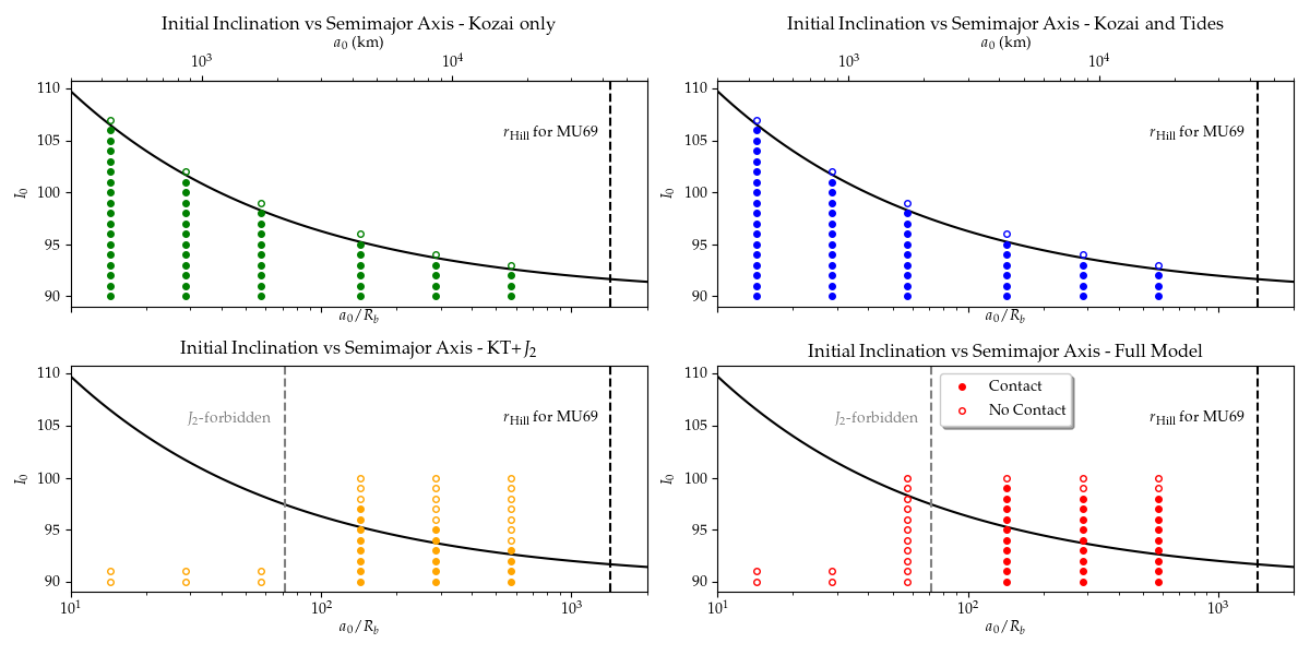
Figure 8.— Mapping of the parameter space of semimajor axis and inclination (for fixed eccentricity $e_{0}=0.1$) over which contact happens. The upper left plots refers to a model with only Kozai oscillations and no dissipation, $J_{2}$ or drag. For this model, the predicted critical inclination is shown as the solid line. The dots represent the simulations we ran. Filled dots represent contact, open dots no contact. The model finds excellent agreement with the prediction (only $I_{0}>90\deg$ is shown but the results are symmetric for prograde orbiters). The upper right plot shows the model of Kozai and dissipation. Because spin-orbit coupling is weak, not much distinction is seen between this and the model of Kozai only. The lower left plot shows a model with Kozai, tides, and $J_{2}$. The quadrupole disrupts Kozai oscillations inside of 0.05 $R_{H}$, but it extends slightly the critical inclination. The lower right plot shows the full model with Kozai, tides, $J_{2}$ and drag. The $J_{2}$-forbidden region still exists, but outside this, the range of inclination over which contact happens is significantly increased.

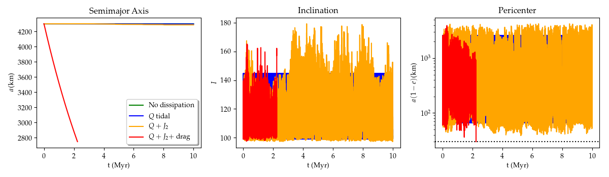
Figure 9.— Evolution for $I_{0}=99^{\circ}$ up to 10 Myr, for simulations with different dynamical terms. The simulation with only the solar terms (green line) leads to regular Kozai oscillations at constant semimajor axis. Including the induced quadrupole (blue line) has little effect. Inclusion of the permanent quadrupole (orange line) leads to irregular Kozai cycles with erratic excursions in inclination and eccentricity. Finally, including the orbital drag leads to a fast decay of semimajor axis, and eventual contact shortly after 2 Myr.

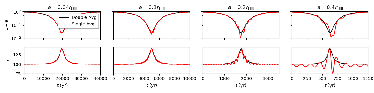
Figure 10.— Comparison between the single and double-averaged secular approximations, for different values of the semimajor axis, shown as a fraction of the Hill radius (0.04, 0.1, 0.2, and 0.4). The upper plots show the eccentricity, the lower plots show the inclination. where the former is averaged over the mean anomaly of the inner binary only, and the latter over the mean anomalies of the inner and outer binaries. The double average is applicable up to 0.1 Hill radii. Beyond that, oscillations on top of the double-averaged solution are seen, increasing amplitude with increasing semimajor axis. These oscillations should make contact more likely as they bring the eccentricity beyond the maximum predicted by the double-averaged model.

4. Conclusion

In this work we present a solution for the two-body problem and for the hierarchical three-body problem with nebular drag, implementing the latter into a Kozai cycles plus tidal friction model. We divide the nebular drag into orbital drag and the sub-Keplerian wind that is effected by the large-scale pressure gradient of the Solar Nebula. The wind is of the order of 50 m/s, whereas the orbital velocity of 10 km bodies is of the order of 10 cm/s. The typical drag timescale for 10 km bodies is of the order of $10$ Myr, but for quadratic drag the wind brings the effective drag timescales down to 0.1 Myr. For linear drag the effect of the wind cancels out and the timescale remains 10 Myr. The regime of quadratic drag corresponds to distances in the asteroid belt, whereas regime of linear drag corresponds to distances in the Kuiper belt. Our model therefore predicts that the asteroid belt should be significantly depleted of pristine binary planetesimals, as nebular drag is effective in bringing them to contact. Observations show that the binary fraction among asteroids is about 15% (Margot et al., 2015) whereas in the Kuiper belt it can be as high as 40% (Noll et al., 2008a, b; Nesvorný, 2011; Fraser et al., 2017). Unfortunately we cannot draw conclusions from these numbers because the asteroid belt is highly collisionally evolved and thus the binary population there is not primordial: only the cold classical population of the Kuiper belt can be used as a diagnostic for initial binary fraction (Morbidelli & Nesvorny, 2019).

For the Kuiper belt, where the drag timescales are of the order of 10 Myr, we find that Kozai-Lidov oscillations are paramount to achieve contact. If the inclination is near 90^∘, the eccentricity of the inner binary increases to near unity and the orbits become grazing. The evolution is characterized by decreasing angular momentum at constant energy, which geometrically means decreasing the semiminor axis while keeping the semimajor axis constant, eventually collapsing the orbit into a straight line (6).

The speed at contact is the orbital velocity; if contact happens at pericenter at high eccentricity, it deviates from the escape velocity only because of the oblateness, independently of the semimajor axis. For MU69, the oblateness leads to a 30% decrease in contact velocity with respect to the escape velocity, the latter scaling with the square root of the density. For mean densities in the range 0.3-0.5 g cm^-3, the contact velocity should be $3.3-4.2$ m s^-1.

The timescale for Kozai cycles for MU69 in the range of semimajor axes of 0.05 to 0.5 Hill radii are at maximum 20 000 years (and as low as 500 years), so contact in this model should have happened right after formation. Considering that the permanent quadrupole $J_{2}$ prevents Kozai oscillations for semimajor axes shorter than 0.05 Hill radii, excluding this “$J_{2}$ forbidden zone” confines contact to a narrow window of the parameter space, in a range of initial inclinations between 85^∘ and 95^∘. Formation by streaming instability (Nesvorný et al., 2019) results in a broad inclination distribution at birth; so the narrow 10^∘ window means that this model predicts that the fraction of contact binaries should be about 5%, which is too on the low end of the observed inclination distribution of KBO binaries (Grundy et al., 2011).

We find that gas drag significantly alters this picture. The permanent quadrupole also has the effect of making the Kozai oscillations stochastic in the range of semimajor axes where they are allowed. This leads to the possibility that the Kozai cycles, previously regular and periodic, can now achieve contact by stochastic fluctuations that nudge the body beyond the allowed region for pure Kozai. Indeed we see this behavior, but very limited when only the quadrupole but no gas is included. The stochastic fluctuations push the window of contact by 1 or 2 degrees beyond the critical inclination of pure Kozai, but no further. When gas drag is included, the window is pushed to the range from 80^∘ to 100^∘. This happens because of a combination of the stochastic fluctuations caused by $J_{2}$ and the fact that gas drag is shrinking the semimajor axis. After a few million years (still within the lifetime of the disk), the semimajor axis has shrunk enough to bring the contact pericenter within reach of the stochastic fluctuations. Together, gas drag and $J_{2}$ can achieve what neither could in isolation. The synergy widens the window of contact to over 10% of the range of inclinations. If the disk is long-lived enough, the window could be pushed to even higher inclinations.

We underscore that our solution naturally provides an explanation to one of the main questions posed by MU69’s nature as a contact binary, in constrast to many cold classicals in the 100 km range that are detached binaries. If the drag time for MU69 is of the order of 10 Myr, an object 10 times bigger would have drag time of 1 Gyr: the effect of nebular drag would be negligible. The situation for 100 km bodies is that of the lower left plot of 8, that depicts Kozai cycles, tides, and the permanent qudrupole, excluding nebular drag, with a narrower window of contact.

As limitations of the work, our KTJD model is accurate only up to the quadrupole approximation. Including the octupole would make the cycles even more chaotic (Naoz, 2016). Also, we use the double-averaged secular approximation, where the motion is averaged in mean anomaly of both the inner and the outer binary. This approximation underestimates the maximum eccentricity and inclination range when compared to the single-average approximation (averaging only in the mean anomaly of the inner binary but resolving the motion of the outer binary) and of course also compared to the exact solution. Both situations potentially increase the region of the parameter space over which contact happens, so our solution may be seen as a conservative lower bound.

Appendix A A: Orbital Solution with Nebular Drag

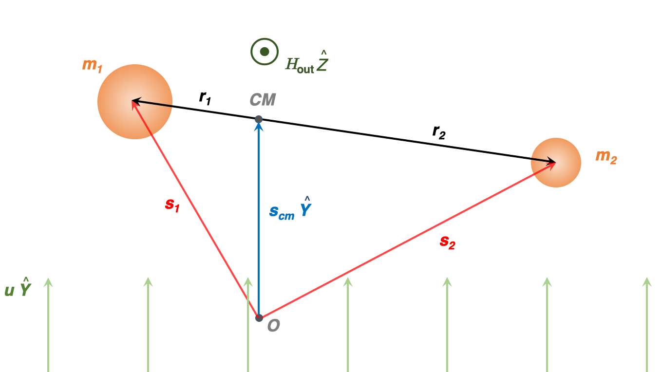
Figure 11.— Geometry of the orbital problem with nebular drag. The masses orbit a common center of mass at distances ${\boldsymbol{r_{1}}}$ and ${\boldsymbol{r_{2}}}$ from it. We choose an arbitrary origin distant ${\boldsymbol{s}}$ from the center of mass, and ${\boldsymbol{s_{1}}}$ and ${\boldsymbol{s_{2}}}$ from the masses. We align the local Hill coordinate $\hat{{\boldsymbol{y}}}$ along the direction of the wind ${\boldsymbol{u}}$, and $\hat{{\boldsymbol{z}}}$ along the direction of the angular momentum of the orbit around the Sun ${\boldsymbol{H}}$.

We consider a binary system of masses $m_{1}$ and $m_{2}$, at distances ${\boldsymbol{s}}_{1}$ and ${\boldsymbol{s}}_{2}$, respectively, from an arbitrary origin (see 11). The bodies are immersed in uniform gas and suffer drag as they orbit. The drag force acts on timescales $\tau_{1}$ and $\tau_{2}$, respectively. We consider that while the binary’s center of mass orbits the Sun at the Keplerian rate $n_{\rm out}$, the gas moves at sub-Keplerian velocity, leading to a uniform headwind on the binary with velocity ${\boldsymbol{u}}$. We distinguish between the orthogonal coordinate systems $\hat{{\boldsymbol{e}}}\hat{{\boldsymbol{q}}}\hat{{\boldsymbol{h}}}$ defined by the orbit and $\hat{{\boldsymbol{x}}}\hat{{\boldsymbol{y}}}\hat{{\boldsymbol{z}}}$, the local Cartesian Hill coordinates where $\hat{{\boldsymbol{x}}}$ points away from the Sun, and $\hat{{\boldsymbol{z}}}$ to the angular momentum vector of the orbit around the Sun. The equations of motion are

$$\ddot{{\boldsymbol{s}}}_{1} = -2n_{\rm out}\left(\hat{{\boldsymbol{z}}}\times\dot{{\boldsymbol{s}}}_{1}\right)-Gm_{2}\frac{\left({\boldsymbol{s}}_{1}-{\boldsymbol{s}}_{2}\right)}{|{\boldsymbol{s}}_{1}-{\boldsymbol{s}}_{2}|^{3}}+3n_{\rm out}^{2}x_{1}\hat{{\boldsymbol{x}}}-\frac{\left(\dot{{\boldsymbol{s}}}_{1}+3/2n_{\rm out}x_{1}\hat{{\boldsymbol{y}}}-{\boldsymbol{u}}\right)}{\tau_{1}}$$ (A1)

$$\ddot{{\boldsymbol{s}}}_{2} = -2n_{\rm out}\left(\hat{{\boldsymbol{z}}}\times\dot{{\boldsymbol{s}}}_{2}\right)-Gm_{1}\frac{\left({\boldsymbol{s}}_{2}-{\boldsymbol{s}}_{1}\right)}{|{\boldsymbol{s}}_{1}-{\boldsymbol{s}}_{2}|^{3}}+3n_{\rm out}^{2}x_{2}\hat{{\boldsymbol{x}}}-\frac{\left(\dot{{\boldsymbol{s}}}_{2}+3/2n_{\rm out}x_{2}\hat{{\boldsymbol{y}}}-{\boldsymbol{u}}\right)}{\tau_{2}}$$ (A2)

where $G$ is the gravitational constant. This system can be reduced to a single particle equivalent as detailed below.

A.1. A.1. Single particle equivalent system

We subtract Eq. (A1) from Eq. (A2), i.e., centering at the primary, and substitute ${\boldsymbol{r}}={\boldsymbol{s}}_{2}-{\boldsymbol{s}}_{1}$ for the distance between the masses. With these operations, the system is

$$\ddot{{\boldsymbol{r}}}=-2n_{\rm out}\left(\hat{{\boldsymbol{z}}}\times\dot{{\boldsymbol{r}}}\right)-\frac{\mu{\boldsymbol{r}}}{r^{3}}+3n_{\rm out}^{2}x\hat{{\boldsymbol{x}}}-\frac{\dot{{\boldsymbol{s}}}_{2}}{\tau_{2}}+\frac{\dot{{\boldsymbol{s}}}_{1}}{\tau_{1}}-\frac{3n_{\rm out}\hat{{\boldsymbol{y}}}}{2}\left(\frac{x_{2}}{\tau_{2}}-\frac{x_{1}}{\tau_{1}}\right)+{\boldsymbol{u}}\left(\frac{1}{\tau_{2}}-\frac{1}{\tau_{1}}\right)$$ (A3)

where $\mu=G(m_{1}+m_{2})$. The bodies’ positions ${\boldsymbol{s}}_{1}$ and ${\boldsymbol{s}}_{2}$ with respect to the origin relate to the barycenter position ${\boldsymbol{s}}_{\rm cm}$ (also with respect to the origin) and the bodies’ positions relative to the barycenter ${\boldsymbol{r}}_{1}$ and ${\boldsymbol{r}}_{2}$ by

$${\boldsymbol{s}}_{1}={\boldsymbol{r}}_{1}+{\boldsymbol{s}}_{\rm cm}\quad{\rm and}\quad{\boldsymbol{s}}_{2}={\boldsymbol{r}}_{2}+{\boldsymbol{s}}_{\rm cm}$$ (A4)

which, given the definition of the barycenter, yields

$${\boldsymbol{r}}_{1}=-\frac{m_{2}}{m_{1}+m_{2}}{\boldsymbol{r}};\quad{\boldsymbol{r}}_{2}=\frac{m_{1}}{m_{1}+m_{2}}{\boldsymbol{r}},$$ (A5)

now substituting ${\boldsymbol{r}}_{1}$ and ${\boldsymbol{r}}_{2}$ as given by Eq. (A4) we have

$$\ddot{{\boldsymbol{r}}}=-2n_{\rm out}\left(\hat{{\boldsymbol{z}}}\times\dot{{\boldsymbol{r}}}\right)-\frac{\mu{\boldsymbol{r}}}{r^{3}}+3n_{\rm out}^{2}x\hat{{\boldsymbol{x}}}-\frac{{\boldsymbol{\dot{r}}}}{\tau_{m}}-\frac{3/2n_{\rm out}x\hat{{\boldsymbol{y}}}}{\tau_{m}}+\frac{{\boldsymbol{u}}-\dot{{\boldsymbol{s}}}_{\rm cm}}{\tau_{w}}$$ (A6)

with the drag timescales

$$\tau_{m}=\frac{\tau_{1}\tau_{2}\ (m_{1}+m_{2})}{\tau_{2}m_{2}+\tau_{1}m_{1}}$$ (A7)

and

$$\tau_{w}=\frac{\tau_{1}\tau_{2}}{\tau_{1}-\tau_{2}}.$$ (A8)

Notice that Eq. (A6) is not yet a single particle equation, as it depends on the motion of the center of mass of the binary. We consider $u\gg\dot{s}_{\rm cm}$ to drop the last term. With this approximation, we can further simplify Eq. (A6) by writing

$$\frac{{\boldsymbol{\dot{r}}}}{\tau_{m}}-\frac{{\boldsymbol{u}}}{\tau_{w}}=\frac{{\boldsymbol{\dot{r}}}-{\boldsymbol{u}}\tau_{m}\tau_{w}^{-1}}{\tau_{m}}$$ (A9)

i.e., the equation of motion becomes a simpler drag equation for a single body, given by

$$\ddot{{\boldsymbol{r}}}=-\frac{\mu{\boldsymbol{r}}}{r^{3}}-\frac{\dot{{\boldsymbol{r}}}-{\boldsymbol{u}}_{\rm eff}}{\tau_{\rm eff}}-2n_{\rm out}\left(\hat{{\boldsymbol{z}}}\times\dot{{\boldsymbol{r}}}\right)+3n_{\rm out}^{2}x\hat{{\boldsymbol{x}}}-\frac{3n_{\rm out}x\hat{{\boldsymbol{y}}}}{2\tau_{\rm eff}}$$ (A10)

with effective wind

$${\boldsymbol{u}}_{\rm eff}={\boldsymbol{u}}\frac{\tau_{m}}{\tau_{w}}={\boldsymbol{u}}\frac{(\tau_{2}-\tau_{1})(m_{1}+m_{2})}{(m_{2}\tau_{2}+m_{1}\tau_{1})}$$ (A11)

and effective drag time $\tau_{\rm eff}=\tau_{m}$.

A.2. A.2. Numerical validation of the single particle equivalent

We show in 12 the evolution of the system Eq. (A1)-Eq. (A2) and that of Eq. (A10). We model the system in a 2D Cartesian box with a wind ${\boldsymbol{u}}=u\hat{{\boldsymbol{y}}}$, and ignoring $n_{\rm out}$. In code units we consider

$$G=1;\quad m_{1}+m_{2}=1;\quad a_{0}=1;\quad n_{0}=1.$$ (A12)

where $a_{0}$ is the initial semimajor axis and $n_{0}$ the initial angular frequency of the binary. We solve the $N$-body with a standard Runge-Kutta scheme 3rd order accurate in time. We take timesteps of $\Delta t=10^{-3}T$, with the period $T=2\pi/n$ dynamically updated as the binary hardens.

To test the code, we consider a binary system of arbitrary masses $m_{1}=0.75$ and $m_{2}=0.25$, drag times $\tau_{1}=3\times 10^{3}$ and $\tau_{2}=10^{3}$, and a wind $u=30$. The masses’ starting positions are given by Eq. (A5) with $|{\boldsymbol{r}}|=a$. The initial orbit is circular with velocities $v_{0i}=n_{0}a_{0i}$.

The simulation is centered at the center of mass and at every full timestep the center of mass position and velocity are reset. The numerical solution of this system, given by Eq. (A1)-Eq. (A2), is shown by the blue solid line in 12.

With these parameters, the one body equivalent (Eq. A10) has effective friction time $\tau_{\rm eff}=1200$ as given by Eq. (A7), and effective wind $u_{\rm eff}=24$, as given by Eq. (A11). The numerical solution of this system, is shown by the red dashed line in 12.

The only difference between these systems is that the single body equivalent is missing the indirect term from the acceleration of the center of mass. As evidenced by the similarity of the solutions, this term is negligible, leading to but a minute deviation in angular momentum and eccentricity toward contact (when the relative distance goes to zero).

Finally, we notice that because the center of mass is accelerated, even though initially the system may have $u\gg\dot{s}_{\rm cm}$, this assumption may not be maintained during the course of the whole simulation. The effect of the wind drag is to try to bring the center of mass velocity to the same velocity as the wind, the situation where the wind drag would cease to exist. The acceleration of the center of mass is given by the center of mass equation

$$\ddot{{\boldsymbol{s}}}_{\rm cm} = \frac{m_{1}\ddot{{\boldsymbol{s}}}_{1}+m_{2}\ddot{{\boldsymbol{s}}}_{2}}{(m_{1}+m_{2})}$$ (A13)

$$= {\boldsymbol{u}}\frac{\tau_{1}m_{2}+\tau_{2}m_{1}}{\tau_{1}\tau_{2}(m_{1}+m_{2})}-\dot{{\boldsymbol{s}}}_{1}\frac{m_{1}}{(m_{1}+m_{2})\tau_{1}}-\dot{{\boldsymbol{s}}}_{2}\frac{m_{2}}{(m_{1}+m_{2})\tau_{2}}$$

If $u\gg\dot{s}_{1,2}$, the wind dominates; the center of mass will accelerate, reaching velocity $u$ within the timescale $\tau_{m}$.

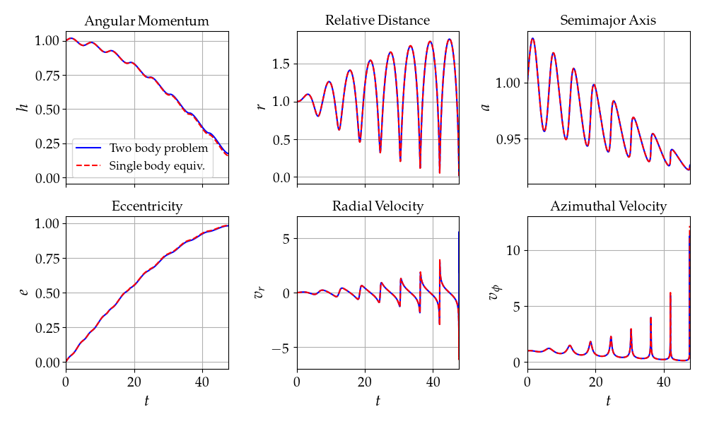
Figure 12.— Comparison between the two massive bodies problem (Eq. (A1)-Eq. (A2), solid blue line), and the equivalent 1-body system with reduced mass and effective wind and drag (Eq. (A10), dashed red line). The 2-body problem has $m_{1}=0.75$ and $m_{2}=0.25$, $\tau_{1}=3\times 10^{3}$ and $\tau_{2}=10^{3}$, and $u=30$. The one-body equivalent has effective friction time $\tau_{\rm eff}=1200$, and effective wind $u_{\rm eff}=24$. The terms with $n_{\rm out}$ are ignored. The agreement is excellent, validating the approximation $u\gg\dot{s}_{\rm cm}$ that motivates Eq. (A10).

A.3. A.3. Orbital solution

Since gravity dominates, we can treat the problem as a Keplerian orbit perturbed by the orbital drag, the wind drag, the Coriolis force, the centrifugal force, and the shear. We use the formalism of Murray & Dermott (1999) to solve for the evolution of semimajor axis, angular momentum, and eccentricity under these forces. Treating the perturbation as

$$d{\boldsymbol{F}}=\overline{R}\hat{{\boldsymbol{r}}}+\overline{T}\hat{{\boldsymbol{\phi}}}+\overline{N}\hat{{\boldsymbol{h}}}$$ (A14)

where $\hat{{\boldsymbol{r}}}$, $\hat{{\boldsymbol{\phi}}}$ are the (cylindrical) unit vectors in the plane of the orbit and $\phi=0$ points at pericenter; that is, $[\hat{{\boldsymbol{r}}},\hat{{\boldsymbol{\phi}}}]$ is $[\hat{{\boldsymbol{e}}},\hat{{\boldsymbol{q}}}]$ rotated by the true anomaly. The solutions for the orbital elements given by (Murray & Dermott, 1999, eqs 2.145, 2.149, 2.150, and 2.157), following Burns (1976)

$$\frac{da}{dt} = \frac{2}{n\sqrt{1-e^{2}}}\ \chi_{a}$$ (A15)

$$\frac{dh}{dt} = \chi_{h}$$ (A16)

$$\frac{de}{dt} = \frac{\sqrt{1-e^{2}}}{na}\ \chi_{e}$$ (A17)

$$\frac{dI}{dt} = \chi_{I}$$ (A18)

$$\frac{d\varOmega}{dt} = \chi_{\varOmega}$$ (A19)

$$\frac{d\omega}{dt} = \frac{\sqrt{1-e^{2}}}{ane}\chi_{\omega}-\chi_{\varOmega}\cos I.$$ (A20)

with the functions $\chi$ given by

$$\chi_{a} = \overline{R}e\sin{f}+\overline{T}\left(1+e\cos{f}\right),$$ (A21)

$$\chi_{h} = r\overline{T},$$ (A22)

$$\chi_{e} = \overline{R}\sin{f}+\overline{T}\left(\cos{f}+\cos{E}\right),$$ (A23)

$$\chi_{I} = r\overline{N}\ \frac{\cos(\omega+f)}{h},$$ (A24)

$$\chi_{\varOmega} = r\overline{N}\ \frac{\sin(\omega+f)}{h\sin I},$$ (A25)

$$\chi_{\omega} = -\overline{R}\cos{f}+\overline{T}\sin f\left(\frac{2+e\cos f}{1+e\cos{f}}\right),$$ (A26)

where $f$ is the true anomaly and $E$ is the eccentric anomaly. We work out the functions $\overline{R}$, $\overline{T}$, and $\overline{N}$ for the several terms involved.

A.3.1 A.3.1. Orbital drag

The orbital drag is

$$\left[\begin{array}[]{c}\overline{R}\\ \overline{T}\\ \overline{N}\end{array}\right]_{\rm drag}=-\frac{1}{\tau}\left[\begin{array}[]{c}\dot{r}\\ r\dot{\phi}\\ 0\end{array}\right],$$ (A27)

for which we will need the solutions for $\dot{r}$ and $r\dot{\phi}$,

$$\dot{r} = \frac{na}{\sqrt{1-e^{2}}}e\sin{f},$$ (A28)

$$r\dot{\phi} = \frac{na}{\sqrt{1-e^{2}}}\left(1+e\cos{f}\right).$$ (A29)

These functions contain terms dependent on the true anomaly, so we take orbital averages to find the secular evolution. We define orbital averages as averages in mean anomaly $M=nt$ according to

$$\left\langle X\right\rangle=\frac{1}{2\pi}\int_{0}^{2\pi}X\ dM$$ (A30)

The series for $\sin{f}$ and $\cos{f}$ are, to 4th order in eccentricity,

$$\sin{f} = \sin M+e\sin 2M+e^{2}\left(\frac{9}{8}\sin 3M-\frac{7}{8}\sin M\right)+e^{3}\left(\frac{4}{3}\sin 4M-\frac{7}{6}\sin 2M\right)$$ (A31)

$$+e^{4}\left(\frac{17}{192}\sin M-\frac{207}{128}\sin 3M+\frac{625}{384}\sin 5M\right)+\mathcal{O}(e^{5})$$

$$\cos{f} = \cos M+e\left(\cos 2M-1\right)+\frac{9e^{2}}{8}\left(\cos 3M+\cos M\right)+\frac{4e^{3}}{3}\left(\cos 4M-\cos 2M\right)$$ (A32)

$$+e^{4}\left(\frac{25}{192}\cos M-\frac{225}{128}\cos 3M+\frac{625}{384}\cos 5M\right)+\mathcal{O}(e^{5})$$

Clearly all terms except $-e$ are periodic, so $\left\langle\cos{f}\right\rangle=-e$ and $\left\langle\sin{f}\right\rangle=0$. The solution for $\cos{E}$ will also be needed, also shown to fourth order in eccentricity

$$\cos{E} = \cos M+\frac{e}{2}\left(\cos 2M-1\right)+\frac{3e^{2}}{8}\left(\cos 3M-\cos M\right)+\frac{e^{3}}{3}\left(\cos 4M-\cos 2M\right)$$ (A33)

$$+e^{4}\left(\frac{5}{192}\cos M-\frac{45}{128}\cos 3M+\frac{125}{384}\cos 5M\right)+\mathcal{O}(e^{5})$$

All terms except $-e/2$ average out over an orbital period, so $\left\langle\cos{E}\right\rangle=-e/2$.

Next we write each perturbation term and find their effect on the evolution of the orbital elements.

Semimajor axis

Substituting Eq. (A28) and Eq. (A29) into Eq. (A27), and plugging into Eq. (A21) yields

$${\chi_{a}}_{,\rm drag}=-\frac{na}{\tau\sqrt{1-e^{2}}}\left(1+2e\cos{f}+e^{2}\right).$$ (A34)

Now taking the orbital average using Eq. (A32), we find the contribution of the orbital drag to the evolution of the semimajor axis

$$\left\langle\chi_{a}\right\rangle_{\rm drag}=-\frac{na}{\tau}\sqrt{1-e^{2}}$$ (A35)

Angular momentum

The angular momentum evolution is given by Eq. (A16), depending only on the azimuthal part $\overline{T}$ of the perturbation. Considering the drag

$$\frac{dh}{dt}=-\frac{h}{\tau}$$ (A36)

Eccentricity

The evolution of eccentricity is given by Eq. (A17) and Eq. (A23). The effect of the drag on the eccentricity is, given Eq. (A27)

$${\chi_{e},}_{\rm drag}=-\frac{na}{\sqrt{1-e^{2}}}\frac{1}{\tau}\left(e+\cos{f}+\cos{E}+e\cos{E}\cos f\right)$$ (A37)

taking the average, $\left\langle\cos{f}\right\rangle=-e$ cancels with $e$. The average $\left\langle\cos{E}\right\rangle=-e/2$, so we have

$$\left\langle\chi_{e}\right\rangle_{\rm drag}=-\frac{na}{\sqrt{1-e^{2}}}\frac{1}{\tau}\left(-e/2+e\left\langle\cos{E}\cos f\right\rangle\right)$$ (A38)

the average $\left\langle\cos{E}\cos{f}\right\rangle$ is found from the equation of the orbit

$$r=a(1-e\cos{E}).$$ (A39)

Multiplying by $\cos{f}$

$$r\cos{f}=a(\cos{f}-e\cos{E}\cos{f})$$ (A40)

given $x_{c}=r\cos{f}$ and averaging

$$\left\langle x_{c}\right\rangle=a(\left\langle\cos{f}\right\rangle-e\left\langle\cos{E}\cos{f}\right\rangle)$$ (A41)

since $\left\langle\cos{f}\right\rangle=-e$ and $\left\langle x_{c}\right\rangle=-3ae/2$, this results in

$$\left\langle\cos{E}\cos{f}\right\rangle=\frac{1}{2}.$$ (A42)

The term in parentheses in Eq. (A38) thus cancels out exactly, so $\left\langle\chi_{e}\right\rangle_{\rm drag}$ = 0 and the orbital drag does not affect the eccentricity.

Inclination

The evolution of inclination is given by Eq. (A18). The orbital drag does not have a normal component, so it cannot affect the inclination.

Longitude of ascending node

The expression for the evolution of the longitude of the ascending node is similar to the one for the inclination. The orbital drag does not have a normal component and thus has no effect.

Argument of Pericenter

The evolution of the argument of pericenter is given by Eq. (A20) and Eq. (A26). For the orbital drag, the contribution is

$${\chi_{\omega},}_{\rm drag}=\frac{2an\sin{f}}{\tau\sqrt{1-e^{2}}}$$ (A43)

which integrates to zero. The orbital drag does not lead to precession.

Orbital Drag: summary

The orbital drag contribution is

$$\left\langle\chi_{a}\right\rangle_{\rm drag} = -\frac{na}{\tau}\sqrt{1-e^{2}}$$ (A44)

$$\left\langle\chi_{h}\right\rangle_{\rm drag} = -\frac{h}{\tau}$$ (A45)

$$\left\langle\chi_{e}\right\rangle_{\rm drag} = 0$$ (A46)

$$\left\langle\chi_{I}\right\rangle_{\rm drag} = 0$$ (A47)

$$\left\langle\chi_{\varOmega}\right\rangle_{\rm drag} = 0$$ (A48)

$$\left\langle\chi_{\omega}\right\rangle_{\rm drag} = 0$$ (A49)

A.3.2 A.3.2. Wind

As for the wind, it is always blowing from the $\hat{{\boldsymbol{y}}}$ direction in Hill Cartesian coordinates ${\boldsymbol{x}}$. We transform between these coordinates and the (Cartesian) orbital plane coordinates ${\boldsymbol{x}}_{\rm cart}=x_{c}\hat{{\boldsymbol{e}}}+y_{c}\hat{{\boldsymbol{q}}}+z_{c}\hat{{\boldsymbol{h}}}$ according to

$${\boldsymbol{x}}_{\rm cart}=\boldsymbol{\mathrm{R}}_{h}(\omega)\boldsymbol{\mathrm{R}}_{e}(I)\boldsymbol{\mathrm{R}}_{h}(\varOmega){\boldsymbol{x}}$$ (A50)

Where $\boldsymbol{\mathrm{R}}_{j}$ is the rotation matrix about axis $j$. To pass to the orbital plane in cylindrical coordinates $\hat{{\boldsymbol{r}}}\hat{{\boldsymbol{\phi}}}\hat{{\boldsymbol{h}}}$, we rotate clockwise around $\hat{{\boldsymbol{h}}}$ by the true anomaly, i.e., ${\boldsymbol{x}}_{\rm cyl}=\boldsymbol{\mathrm{R}}_{h}(-f){\boldsymbol{x}}_{\rm cart}$. We thus have

$${\boldsymbol{x}}_{\rm cyl}=\boldsymbol{\mathrm{R}}{\boldsymbol{x}}=\boldsymbol{\mathrm{R}}_{h}(\omega-f)\boldsymbol{\mathrm{R}}_{e}(I)\boldsymbol{\mathrm{R}}_{h}(\varOmega){\boldsymbol{x}}$$ (A51)

where $\boldsymbol{\mathrm{R}}=\boldsymbol{\mathrm{R}}_{h}(\omega-f)\boldsymbol{\mathrm{R}}_{e}(I)\boldsymbol{\mathrm{R}}_{h}(\varOmega)$ is the full rotation matrix for the transformation. For the wind, the vector is in the $\hat{{\boldsymbol{y}}}$ direction; for completeness we give the transformations of the local Hill coordinate unit vectors $\hat{{\boldsymbol{x}}}=[1,0,0]^{T}$, $\hat{{\boldsymbol{y}}}=[0,1,0]^{T}$, and $\hat{{\boldsymbol{z}}}=[0,0,1]^{T}$ to the coordinate system $\hat{{\boldsymbol{r}}}\hat{{\boldsymbol{\phi}}}\hat{{\boldsymbol{h}}}$ of the binary orbit

$$R\hat{{\boldsymbol{x}}}=\left[\begin{array}[]{c}\cos I\sin\varOmega\sin{\left(f-\omega\right)}+\cos{\left(f-\omega\right)}\cos\varOmega\\ -\cos\varOmega\sin{\left(f-\omega\right)}+\cos I\sin\varOmega\cos{\left(f-\omega\right)}\\ \sin\varOmega\sin I\end{array}\right],$$ (A52)

$$R\hat{{\boldsymbol{y}}}=\left[\begin{array}[]{c}\cos I\cos\varOmega\sin{\left(f-\omega\right)}-\cos{\left(f-\omega\right)}\sin\varOmega\\ \sin\varOmega\sin{\left(f-\omega\right)}+\cos I\cos\varOmega\cos{\left(f-\omega\right)}\\ \cos\varOmega\sin I\end{array}\right],$$ (A53)

and

$$R\hat{{\boldsymbol{z}}}=\left[\begin{array}[]{c}-\sin I\sin{\left(f-\omega\right)}\\ -\sin I\cos{\left(f-\omega\right)}\\ \cos I\end{array}\right].$$ (A54)

Thus, for the wind

$$\left[\begin{array}[]{c}\overline{R}\\ \overline{T}\\ \overline{N}\end{array}\right]_{\rm wind}=-\frac{u}{\tau}\left[\begin{array}[]{c}\cos I\cos\varOmega\sin{\left(f-\omega\right)}-\cos{\left(f-\omega\right)}\sin\varOmega\\ \sin\varOmega\sin{\left(f-\omega\right)}+\cos I\cos\varOmega\cos{\left(f-\omega\right)}\\ \cos\varOmega\sin I\end{array}\right].$$ (A55)

Semimajor axis

The influence on the semimajor axis, given by Eq. (A21), is

$$\chi_{a,_{\rm wind}}=\cos I\cos\varOmega\left[\cos{\left(f-\omega\right)}+e\cos\omega\right]+\sin\varOmega\left[\sin{\left(f-\omega\right)}-e\sin\omega\right]$$ (A56)

Taking the orbital average,

$$\left\langle\cos{\left(f-\omega\right)}\right\rangle = \left\langle\cos f\right\rangle\cos\omega+\left\langle\sin f\right\rangle\cos\omega=-e\cos\omega,$$ (A57)

$$\left\langle\sin{\left(f-\omega\right)}\right\rangle = \left\langle\sin f\right\rangle\cos\omega-\left\langle\cos f\right\rangle\sin\omega=e\sin\omega.$$ (A58)

Averaged in the inner orbit, all terms in Eq. (A56) cancel, i.e.

$$\left\langle\chi_{a}\right\rangle_{\rm wind}=0.$$ (A59)

The external wind has no secular effect on the semimajor axis.

Angular momentum

For the wind

$$\frac{dh}{dt} = -\frac{u}{\tau}r\left[\sin\varOmega\sin{\left(f-\omega\right)}+\cos I\cos\varOmega\cos{\left(f-\omega\right)}\right]$$ (A60)

$$= -\frac{u}{\tau}\left[\sin\varOmega(y\cos\omega-x\sin\omega)+\cos I\cos\varOmega(x\cos\omega+y\sin\omega)\right]$$ (A61)

where $x=r\cos{f}$ and $y=r\sin{f}$ are the Cartesian coordinates in the reference frame of the orbit. Given the Keplerian solution, they are $x=a(\cos E-e)$ and $y=a\sin E$. Using the expansion for $E$, it results in $\left\langle x\right\rangle=-3ae/2$ and $\left\langle y\right\rangle=0.$ So,

$$\frac{d\left\langle h\right\rangle}{dt}=-ae\frac{3u}{2\tau}\left(\cos I\cos\varOmega\cos\omega-\sin\varOmega\sin\omega\right)$$ (A62)

Eccentricity

For the wind, according to Eq. (A55)

$${\chi_{e}}_{,{\rm wind}}=\frac{u}{\tau}\left\{\cos I\cos\varOmega\left[\cos E\cos{\left(f-\omega\right)}+\cos\omega\right]+\sin\varOmega\left[\cos E\sin{\left(f-\omega\right)}-\sin\omega\right]\right\}$$ (A63)

given $\left\langle\cos{E}\cos{f}\right\rangle=1/2$ and $\left\langle\cos{E}\sin{f}\right\rangle=0$, the average over $f$ is

$$\left\langle\chi_{e}\right\rangle_{\rm wind}=\frac{3u}{2\tau}\left(\cos I\cos\varOmega\cos\omega-\sin\varOmega\sin\omega\right)$$ (A64)

The evolution of the orbitally-averaged eccentricity is thus due to the wind only, according to

$$\frac{d\left\langle e\right\rangle}{dt}=\frac{\sqrt{1-e^{2}}}{na}\ \frac{3u}{2\tau}\ \left(\cos I\cos\varOmega\cos\omega-\sin\varOmega\sin\omega\right)$$ (A65)

Inclination

The evolution of inclination is given by Eq. (A18). For the wind

$$\frac{dI}{dt}=-\frac{u}{h\tau}a\cos\varOmega\sin I\left[\cos(f+\omega)\right](1-e\cos E)$$ (A66)

This expression expands to

$$\frac{dI}{dt}=-\frac{u}{h\tau}a\cos\varOmega\sin I\left(\cos\omega\cos{f}-\sin\omega\sin{f}-e\cos\omega\cos E\cos f+e\sin\omega\cos E\sin f\right)$$ (A67)

On averaging, the second and last terms in parentheses cancel out. The first and third terms add up to $-3/2ae\cos\omega$ . The evolution of the orbit-averaged inclination due to the wind is thus

$$\frac{d\left\langle I\right\rangle}{dt}=\frac{3u}{2\tau}\frac{ae}{h}\cos\varOmega\cos\omega\sin I$$ (A68)

Longitude of ascending node

The effect of the wind is

$$\frac{d\varOmega}{dt}=-\frac{u}{h\tau}a\cos\varOmega\sin(f+\omega)(1-e\cos E)$$ (A69)

which expands to

$$\frac{d\varOmega}{dt}=-\frac{u}{h\tau}a\cos\varOmega\left(\cos\omega\sin f+\sin\omega\cos f-e\cos\omega\cos E\sin f-e\sin\omega\cos E\cos f\right)$$ (A70)

On averaging, the first and third terms in parentheses cancel out. The second and last terms add up to $-3/2ae\sin\omega$. The evolution of the orbit-averaged longitude of ascending node is thus

$$\frac{d\left\langle\varOmega\right\rangle}{dt}=\frac{3u}{2\tau}\frac{ae}{h}\cos\varOmega\sin\omega.$$ (A71)

Argument of Pericenter

The evolution of the argument of pericenter is given by Eq. (A20) and Eq. (A26). For the wind

$$\chi_{\omega} = \frac{u}{\tau}\left\{\cos{f}\left[\cos I\cos\varOmega\sin{\left(f-\omega\right)}-\cos{\left(f-\omega\right)}\sin\varOmega\right]\right.$$ (A72)

$$\left.-\left(\frac{2+e\cos{f}}{1+e\cos{f}}\right)\sin{f}\left[\sin\varOmega\sin{\left(f-\omega\right)}+\cos I\cos\varOmega\cos{\left(f-\omega\right)}\right]\right\}$$

we expand and group the terms as

$$\chi_{\omega} = \frac{u}{\tau}\left\{-(\cos{I}\cos{\Omega}\sin{\omega}+\cos{\omega}\sin{\Omega})\left[\cos^{2}f+\sin^{2}f\left(\frac{2+e\cos{f}}{1+e\cos{f}}\right)\right]\right.$$ (A73)

$$\left.+(\cos{I}\cos{\Omega}\cos{\omega}-\sin{\Omega}\sin{\omega})\left[1-\left(\frac{2+e\cos{f}}{1+e\cos{f}}\right)\right]\cos{f}\sin{f}\right\}$$

upon integration the second term is periodic in $M$ and cancels. We are left with

$$\chi_{\omega}=\frac{u}{\tau}\left(\cos{I}\cos{\Omega}\sin{\omega}+\cos{\omega}\sin{\Omega}\right)A(e)$$ (A74)

where

$$A(e)=-\left\langle\cos^{2}f\right\rangle-\left\langle\sin^{2}f\left(\frac{2+e\cos{f}}{1+e\cos{f}}\right)\right\rangle$$ (A75)

a function of the eccentricity alone. The orbital evolution of the argument of pericenter is thus

$$\frac{d\left\langle\omega\right\rangle}{dt}=\frac{u}{\tau}\frac{\sqrt{1-e^{2}}}{ane}\left\{\left[A(e)-\frac{3}{2}\frac{ae}{h}\right]\cos I\cos\varOmega\sin\omega+A(e)\cos\omega\sin\varOmega\right\}$$ (A76)

Wind: summary

The external wind contribution is

$$\left\langle\chi_{a}\right\rangle_{\rm wind} = 0$$ (A77)

$$\left\langle\chi_{h}\right\rangle_{\rm wind} = -ae\frac{3u}{2\tau}\left(\cos I\cos\varOmega\cos\omega-\sin\varOmega\sin\omega\right)$$ (A78)

$$\left\langle\chi_{e}\right\rangle_{\rm wind} = \frac{\sqrt{1-e^{2}}}{na}\ \frac{3u}{2\tau}\ \left(\cos I\cos\varOmega\cos\omega-\sin\varOmega\sin\omega\right)$$ (A79)

$$\left\langle\chi_{I}\right\rangle_{\rm wind} = \frac{3u}{2\tau}\frac{ae}{h}\cos\varOmega\cos\omega\sin I$$ (A80)

$$\left\langle\chi_{\varOmega}\right\rangle_{\rm wind} = \frac{3u}{2\tau}\frac{ae}{h}\cos\varOmega\sin\omega$$ (A81)

$$\left\langle\chi_{\omega}\right\rangle_{\rm wind} = \frac{u}{\tau}\left(\cos{I}\cos{\Omega}\sin{\omega}+\cos{\omega}\sin{\Omega}\right)A(e)$$ (A82)

A.3.3 A.3.3. Coriolis force

The Coriolis force, being an inertial force, cannot alter the energy or angular momentum of the orbit. As a consequence, eccentricity is also unmodified. Its effect is to lead to an apparent precession of the orbit in the Hill co-rotating coordinate frame. We work out the perturbations introduced by the Coriolis Given Eqs. A54

$$\left[\begin{array}[]{c}\overline{R}\\ \overline{T}\\ \overline{N}\end{array}\right]_{\rm Coriolis}=2n_{\rm out}\left[\begin{array}[]{c}r\dot{\phi}\cos I\\ -\dot{r}\cos I\\ r\dot{\phi}\sin I\sin{\left(f-\omega\right)}-\dot{r}\sin I\cos{\left(f-\omega\right)}\end{array}\right]$$ (A83)

Semimajor axis

For the semimajor axis, using Eq. (A21),

$${\chi_{h},}_{\rm Coriolis}=2n_{\rm out}\cos I\left[r\dot{\phi}e\sin{f}-\dot{r}\left(1+e\cos{f}\right)\right]$$ (A84)

and given Eq. (A28) and Eq. (A29) the two terms cancel identically: $\chi_{a}=0$.

Angular momentum

The influence of the Coriolis force on angular momentum is

$${\chi_{h},}_{\rm Coriolis}=-\frac{2n_{\rm out}na^{2}e\cos I}{\sqrt{1-e^{2}}}\left(1-e\cos{E}\right)\sin{f}$$ (A85)

which is a periodic function of $M$ and integrates to zero.

Eccentricity

The influence of the Coriolis force on eccentricity is

$${\chi_{e},}_{\rm Coriolis}=\frac{2n_{\rm out}na\cos I}{\sqrt{1-e^{2}}}\left(1-e\cos{E}\right)\sin{f}$$ (A86)

which is a periodic function of $M$ and integrates to zero.

Inclination

The influence of the Coriolis force on inclination is

$${\chi_{I},}_{\rm Coriolis}=-\frac{2n_{\rm out}na^{2}\sin I}{\sqrt{1-e^{2}}}[e\sin\omega-\sin(f-\omega)]\cos(f+\omega)(1-e\cos{E})$$ (A87)

The product $\sin(f-\omega)\cos(f+\omega)=\cos{f}\sin{f}-\cos\omega\sin\omega$, so

$${\chi_{I},}_{\rm Coriolis}=-\frac{2n_{\rm out}na^{2}\sin I}{\sqrt{1-e^{2}}}\psi_{I}$$ (A88)

where

$$\psi_{I}=[(1+e\cos{f})\sin\omega\cos\omega-e\sin\omega^{2}\sin{f}-\cos{f}\sin{f}](1-e\cos{E}).$$ (A89)

And, expanding these terms,

$$\psi_{I} = (1+e\cos{f}-e\cos{E}-e^{2}\cos{f}\cos{E})\sin\omega\cos\omega$$ (A90)

$$-e\sin\omega^{2}\sin{f}-\cos{f}\sin{f}+e2\sin\omega^{2}\cos{E}\sin{f}-e\cos{E}\cos{f}\sin{f}$$

Integrating, all terms but the first one cancel out, leaving only

$$\left\langle\psi_{I}\right\rangle=(1-e^{2})\sin\omega\cos\omega$$ (A91)

The evolution of inclination due to the Coriolis force is thus

$${\chi_{I},}_{\rm Coriolis}=-2n_{\rm out}na^{2}\sqrt{1-e^{2}}\sin I\sin\omega\cos\omega$$ (A92)

Longitude of ascending node

The influence of the Coriolis force on the longitude of the ascending node is

$${\chi_{\varOmega},}_{\rm Coriolis}=-\frac{2n_{\rm out}na^{2}}{\sqrt{1-e^{2}}}[e\sin\omega-\sin(f-\omega)]\sin(f+\omega)(1-e\cos{E})$$ (A93)

The product $\sin(f-\omega)\sin(f+\omega)=-1/2\cos 2f+1/2\cos 2\omega$, so

$${\chi_{\varOmega},}_{\rm Coriolis}=-\frac{2n_{\rm out}na^{2}}{\sqrt{1-e^{2}}}\psi_{\varOmega}$$ (A94)

where $\psi_{\varOmega}=(e\sin{f}\cos\omega\sin\omega+e\sin^{2}\omega\cos{f}+1/2\cos 2f-1/2\cos 2\omega)(1-e\cos{E})$

expanding these terms,

$$\psi_{\varOmega} = e\sin\omega\cos\omega\sin{f}+e\sin^{2}\omega\cos{f}+1/2\cos 2f-1/2\cos 2\omega$$ (A95)

$$-e^{2}\sin\omega\cos\omega\sin{f}\cos{E}-e^{2}\sin^{2}\omega\cos{f}\cos{E}-e\cos{E}\cos 2f/2+e\cos{E}\cos 2\omega/2$$

Integrating, we are left with

$$\left\langle\psi_{\varOmega}\right\rangle=\frac{1}{2}\left[-3e^{2}\sin 2\omega-\left(1+\frac{e^{2}}{2}\right)\cos 2\omega+\left\langle\frac{r}{a}\cos 2f\right\rangle\right]$$ (A96)

writing

$$B(e)=\left\langle\frac{r}{a}\cos 2f\right\rangle$$ (A97)

the evolution of longitude of ascending node due to the Coriolis force is

$${\chi_{\varOmega},}_{\rm Coriolis}=-\frac{n_{\rm out}na^{2}}{\sqrt{1-e^{2}}}\left[-3e^{2}\sin 2\omega-\left(1+\frac{e^{2}}{2}\right)\cos 2\omega+B(e)\right]$$ (A98)

Argument of Pericenter

The evolution of the argument of pericenter is given by

$${\chi_{\omega},}_{\rm Coriolis}=-\frac{2n_{\rm out}na\cos I}{\sqrt{1-e^{2}}}\psi_{\omega}$$ (A99)

with

$$\psi_{\omega}=\cos{f}+e\cos^{2}f+e\sin^{2}f\left(\frac{2+e\cos{f}}{1+e\cos{f}}\right)$$ (A100)

upon integration

$$\left\langle\psi_{\omega}\right\rangle=-e+e\left\langle\cos^{2}f\right\rangle+e\left\langle\sin^{2}f\left(\frac{2+e\cos{f}}{1+e\cos{f}}\right)\right\rangle$$ (A101)

a function of the eccentricity alone. The evolution of the argument of pericenter is thus

$${\chi_{\omega},}_{\rm Coriolis}=-\frac{2n_{\rm out}na\cos I}{\sqrt{1-e^{2}}}C(e)$$ (A102)

where $C(e)=\left\langle\psi_{\omega}\right\rangle$.

Coriolis force: summary

The Coriolis force contribution is

$$\left\langle\chi_{a}\right\rangle_{\rm Coriolis} = 0$$ (A103)

$$\left\langle\chi_{h}\right\rangle_{\rm Coriolis} = 0$$ (A104)

$$\left\langle\chi_{e}\right\rangle_{\rm Coriolis} = 0$$ (A105)

$$\left\langle\chi_{I}\right\rangle_{\rm Coriolis} = -2n_{\rm out}na^{2}\sqrt{1-e^{2}}\sin I\sin\omega\cos\omega$$ (A106)

$$\left\langle\chi_{\varOmega}\right\rangle_{\rm Coriolis} = -\frac{n_{\rm out}na^{2}}{\sqrt{1-e^{2}}}\left[-3e^{2}\sin 2\omega-\left(1+\frac{e^{2}}{2}\right)\cos 2\omega+B(e)\right]$$ (A107)

$$\left\langle\chi_{\omega}\right\rangle_{\rm Coriolis} = -\frac{2n_{\rm out}na\cos I}{\sqrt{1-e^{2}}}C(e)$$ (A108)

A.4. A.4. Orbital Evolution

Putting it all together (ignoring centrifugal force and shear)

$$\frac{d\left\langle a\right\rangle}{dt} = -\frac{2\left\langle a\right\rangle}{\tau};$$ (A109)

$$\frac{d\left\langle e\right\rangle}{dt} = \frac{\sqrt{1-e^{2}}}{na}\frac{3u}{2\tau}\left(\cos I\cos\varOmega\cos\omega-\sin\varOmega\sin\omega\right);$$ (A110)

$$\frac{d\left\langle h\right\rangle}{dt} = -\frac{\left\langle h\right\rangle}{\tau}-ae\frac{3u}{2\tau}\left(\cos I\cos\varOmega\cos\omega-\sin\varOmega\sin\omega\right);$$ (A111)

$$\frac{d\left\langle I\right\rangle}{dt} = \frac{3u}{2\tau}\frac{ae}{h}\cos\varOmega\cos\omega\sin I-2n_{\rm out}na^{2}\sqrt{1-e^{2}}\sin I\sin\omega\cos\omega;$$ (A112)

$$\frac{d\left\langle\varOmega\right\rangle}{dt} = \frac{3u}{2\tau}\frac{ae}{h}\cos\varOmega\sin\omega-\frac{n_{\rm out}na^{2}}{\sqrt{1-e^{2}}}\left[-3e^{2}\sin 2\omega-\left(1+\frac{e^{2}}{2}\right)\cos 2\omega+B(e)\right];$$ (A113)

$$\frac{d\left\langle\omega\right\rangle}{dt} = \frac{\sqrt{1-e^{2}}}{ane}\left\{\frac{u}{\tau}\left[A(e)-\frac{3}{2}\frac{ae}{h}\right]\left[\cos I\cos\varOmega\sin\omega+A(e)\cos\omega\sin\varOmega\right]\right.$$

$$\left.-\frac{2n_{\rm out}na\cos I}{\sqrt{1-e^{2}}}C(e)+\frac{2n_{\rm out}na^{2}\cos I}{\sqrt{1-e^{2}}}\left[-\frac{3}{2}e^{2}\sin 2\omega-\frac{1}{2}\left(1+\frac{e^{2}}{2}\right)\cos 2\omega+\frac{B(e)}{2}\right]\right\}.$$

The system is over-specified because $a$ and $h$ define the eccentricity. Still we keep the equation for $h$ for physical insight.

A.4.1 A.4.1. Isolated binary ($n_{\rm out}=0$)

Let us consider first the case where $n_{\rm out}=0$, i.e., an isolated binary not in orbit around the Sun. The equations reduce to

$$\frac{d\left\langle a\right\rangle}{dt} = -\frac{2\left\langle a\right\rangle}{\tau};$$ (A115)

$$\frac{d\left\langle e\right\rangle}{dt} = \frac{\sqrt{1-e^{2}}}{na}\frac{3u}{2\tau}\left(\cos I\cos\varOmega\cos\omega-\sin\varOmega\sin\omega\right);$$ (A116)

$$\frac{d\left\langle h\right\rangle}{dt} = -\frac{\left\langle h\right\rangle}{\tau}-ae\frac{3u}{2\tau}\left(\cos I\cos\varOmega\cos\omega-\sin\varOmega\sin\omega\right);$$ (A117)

$$\frac{d\left\langle I\right\rangle}{dt} = \frac{3u}{2\tau}\frac{ae}{h}\cos\varOmega\cos\omega\sin I;$$ (A118)

$$\frac{d\left\langle\varOmega\right\rangle}{dt} = \frac{3u}{2\tau}\frac{ae}{h}\cos\varOmega\sin\omega;$$ (A119)

$$\frac{d\left\langle\omega\right\rangle}{dt} = \frac{\sqrt{1-e^{2}}}{ane}\left[\left(A(e)-\frac{3u}{2\tau}\frac{ae}{h}\right)\cos I\cos\varOmega\sin\omega+A(e)\cos\omega\sin\varOmega\right].$$ (A120)

For an orbit originally at $\varOmega=\omega=0$, the derivatives of $\left\langle\varOmega\right\rangle$, and $\left\langle\omega\right\rangle$ vanish. This is a remarkable effect: there is no precession of the argument of pericenter or longitude of the ascending node for this choice of parameters. The system reduces to

$$\frac{d\left\langle a\right\rangle}{dt} = -\frac{2\left\langle a\right\rangle}{\tau};$$ (A121)

$$\frac{d\left\langle e\right\rangle}{dt} = \frac{\sqrt{1-e^{2}}}{na}\frac{3u}{2\tau}\cos I;$$ (A122)

$$\frac{d\left\langle h\right\rangle}{dt} = -\frac{\left\langle h\right\rangle}{\tau}-ae\frac{3u}{2\tau}\cos I;$$ (A123)

$$\frac{d\left\langle I\right\rangle}{dt} = \frac{3u}{2\tau}\frac{ae}{h}\sin I;$$ (A124)

which is not decoupled because eccentricity and inclination depend on each other. For zero initial inclination the derivative of $\left\langle I\right\rangle$ also cancels, and the system further reduces to

$$\frac{d\left\langle a\right\rangle}{dt} = -\frac{2\left\langle a\right\rangle}{\tau};$$ (A125)

$$\frac{d\left\langle e\right\rangle}{dt} = \frac{\sqrt{1-e^{2}}}{na}\frac{3u}{2\tau};$$ (A126)

$$\frac{d\left\langle h\right\rangle}{dt} = -\frac{\left\langle h\right\rangle}{\tau}-ae\frac{3u}{2\tau}.$$ (A127)

This is a system that loses energy in a slow timescale given by $\tau/2$, whereas the angular momentum decreases (thus eccentricity increases) in the faster timescale given by the wind. The general solution for $I=\varOmega=\omega=0$ is

$$\left\langle a(t)\right\rangle = a_{0}\mathrm{e}^{-2t/\tau};$$ (A128)

$$\left\langle e(t)\right\rangle = \cos\left[\cos^{-1}\left(e_{0}\right)+\frac{3u}{2}\sqrt{\frac{a_{0}}{\mu}}\left(1-\mathrm{e}^{-t/\tau}\right)\right];$$ (A129)

$$\left\langle h(t)\right\rangle = \mathrm{e}^{-t/\tau}\left\{h_{0}-1+\cos\left[\frac{3}{2}a_{0}u\left(1-\mathrm{e}^{-t/\tau}\right)\right]\right\};$$ (A130)

which we show graphically in 13, the agreement between the analytical and numerical solutions is excellent.

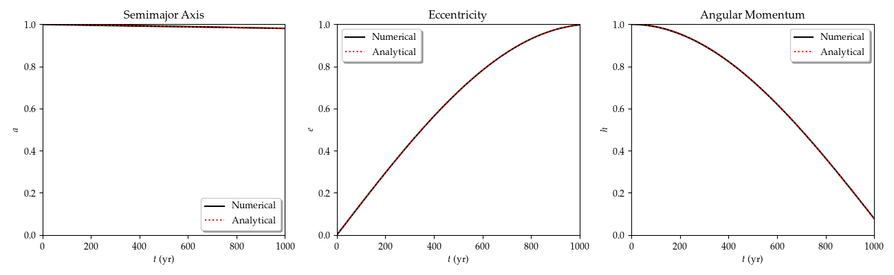
Figure 13.— The evolution of an isolated binary under influence of wind and orbital drag. The wind drives angular momentum loss while it has no effect on the energy (which is dissipated via orbital drag). The effect is rapid eccentricity growth at nearly constant semimajor axis. Contact happens when the eccentricity nears one. The numerical calculation is in excellent agreement with the analytical solution Eqs. (A128)–(A130).

A.4.2 A.4.2. Hierarchical binary ($n_{\rm out}\neq 0$)

For an orbit originally at $\varOmega=\omega=0$, the derivatives of $\left\langle\varOmega\right\rangle$, and $\left\langle\omega\right\rangle$ are

$$\frac{d\left\langle\varOmega\right\rangle}{dt} = \frac{n_{\rm out}na^{2}}{\sqrt{1-e^{2}}}D(e);$$ (A131)

$$\frac{d\left\langle\omega\right\rangle}{dt} = n_{\rm out}F(e)\cos I.$$ (A132)

$$D(e) = \left[\left(1+\frac{e^{2}}{2}\right)-B(e)\right]$$ (A133)

$$F(e) = \frac{1}{e}\left[-\left(1+\frac{e^{2}}{2}\right)+B(e)\right]+C(e)$$ (A134)

if $e$ and $I$ are slow-growing, then $\omega=F(e)\cos I\ n_{\rm out}t$. The mean anomaly of the outer orbit $M_{\rm out}=n_{\rm out}t$ is thus related to the argument of pericenter.

$$\omega=F(e)\cos I\ M_{\rm out}$$ (A135)

Thus, if eccentricity and inclination are slow growing in comparison to $M_{\rm out}$ we can approximate

$$d\omega\approx F(e)\cos I\ dM_{\rm out}$$ (A136)

if we define an average over the solar period,

$$\tilde{X}=\frac{1}{2\pi}\int_{0}^{2\pi}XdM_{\rm out}$$ (A137)

This average can be related to an average in argument of pericenter

$$\tilde{X}=\frac{1}{2\pi F(e)\cos I}\int_{0}^{2\pi}Xd\omega$$ (A138)

Thus, averaging over a precession period (related to the solar period), the equations for the other parameters reduce to

$$\frac{d\tilde{a}}{dt} = -\frac{2\tilde{a}}{\tau};$$ (A139)

$$\frac{d\tilde{e}}{dt} = 0;$$ (A140)

$$\frac{d\tilde{h}}{dt} = -\frac{\tilde{h}}{\tau};$$ (A141)

$$\frac{d\tilde{I}}{dt} = 0.$$ (A142)

the eccentricity and inclination variation cancel out, as well as the wind term in the angular momentum evolution. During a solar orbit period, the wind makes the eccentricity grow and angular momentum decay for half the orbit, and then decrease by the same amount in the other half. Energy and angular momentum decay at the timescale of orbital drag $\tau$ while keeping the eccentricity constant. This behavior is shown in 14. Averaged over orbital and solar period, only the orbital drag remains and the solution is simply

$$\tilde{a} = a_{0}\mathrm{e}^{-2t/\tau};$$ (A143)

$$\tilde{e} = e_{0};$$ (A144)

$$\tilde{h} = h_{0}\mathrm{e}^{-t/\tau};$$ (A145)

$$\tilde{I} = I_{0}.$$ (A146)

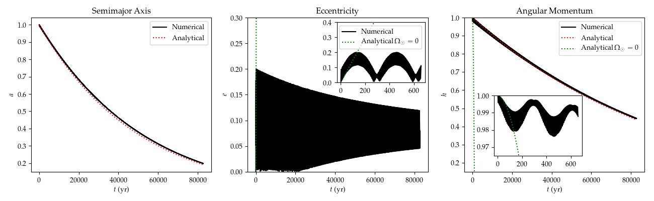
Figure 14.— Evolution considering the orbit around the Sun. As the direction of the wind changes with respected to the fixed eccentricity vector of the binary, for half of the solar orbit the eccentricity grows as predicted by the isolated binary solution, and for the other half it decreases by the same amount. Similarly, the angular momentum decreases by the wind, and then increases in the other half of the orbit. Averaged over the solar period, the solution is described by a simple orbital drag solution $a=a_{0}\mathrm{e}^{-2t/\tau}$, $e\equiv{\rm const}$ and $h=h_{0}\mathrm{e}^{-t/\tau}$.

Appendix B B. Drag Time

When the mean free path of the gas is much smaller than the object, the gas can be treated like a fluid and viscous interactions at the surface of the body lead to the emergence of drag. The mean free path is

$$\lambda_{\rm mfp}=\frac{\mu_{\rm mol}m_{H}}{\rho\sigma_{\rm coll}}$$ (B1)

where $\sigma_{\rm coll}=2\times 10^{-15}\,{\rm cm}^{2}$ is the collisional cross section of molecular hydrogen, $\mu_{\rm mol}=2.3$ is the mean molecular weight for a 5:2 hydrogen to helium mixture, $\rho$ is the gas volume density, and $m_{H}$ stands for the atomic mass unit.

Using the MMSN temperature and column density (Weidenschilling, 1977; Hayashi, 1981; Chiang & Goldreich, 1997)

$${\rm T} = 280\,{\rm K}\ \left(\frac{r}{1\,{\rm AU}}\right)^{-0.5}$$ (B2)

$$\Sigma = 1700\,{\rm g\,cm}^{-2}\left(\frac{r}{1\,{\rm AU}}\right)^{-1.5},$$ (B3)

one finds $\lambda_{\rm mfp}=0.5$ km at 45 AU in the MMSN, and the drag regime of continuous flow is valid. This regime splits into two regimes depending on the Reynolds number, linear and quadratic, with a smooth transition in between. Stokes drag happens for small Reynolds number ($\mathrm{Re}\lesssim 1$ ), where the drag is dominated by viscosity at the surface of the body. The transition to quadratic drag happens at high Reynolds numbers ($\mathrm{Re}\gtrsim 800$), where ram pressure dominates. The Reynolds number is

$$\mathrm{Re}=2R\rho|\Delta{\boldsymbol{v}}|/\mu_{\rm visc},$$ (B4)

where $\Delta{\boldsymbol{v}}$ is the relative velocity between the body and the gas and

$$\mu_{\rm visc}=\sqrt{\frac{8}{9\pi}}\rho c_{s}\lambda_{\rm mfp}$$ (B5)

is the dynamical viscosity, with $c_{s}$ being the sound speed. Substituting this expression into $\mathrm{Re}$, with $\Delta v=\eta v_{k}$ for the wind, leads to

$$\mathrm{Re} = \frac{3}{4}\left|\frac{\partial\ln P}{\partial\ln r}\right|\frac{\sigma_{\rm coll}}{m_{H}}\frac{R}{\mu_{\rm mol}}\frac{\Sigma}{r}$$

$$\approx 3\left|\frac{\partial\ln P}{\partial\ln r}\right|\left(\frac{R}{10\,{\rm km}}\right)\left(\frac{\mu_{\rm mol}}{2}\right)^{-1}\left(\frac{\varSigma}{5\,{\rm g\,cm^{-2}}}\right)\left(\frac{r}{45\,{\rm AU}}\right)^{-1-p}$$

where $p\equiv-\partial\ln\Sigma/\partial\ln r$ is the power law of the column density, positively defined. For the MMSN, $\mathrm{Re}\approx 10$ at 45 AU, and thus we are very close to Stokes law. The drag time is

$$\tau=\frac{4\lambda_{\rm mfp}\rho_{\bullet}}{3\rho C_{D}c_{s}}\frac{1}{\mathrm{Ma}\mathrm{Kn}}$$ (B7)

where $\mathrm{Kn}=\lambda_{\rm mfp}/2R$ is the Knudsen number and $\mathrm{Ma}=|\Delta{\boldsymbol{v}}|/c_{s}$ the flow Mach number. For Stokes flow at low Reynolds number $C_{D}=24/\mathrm{Re}$, leading to

$$\tau=\frac{16}{18}\frac{\rho_{\bullet}R^{2}}{c_{s}}\frac{\sigma_{\rm coll}}{\mu m_{H}}.$$ (B8)

The resulting drag times are $\tau_{1}=4.72\times 10^{7}$ yr and $\tau_{2}=3.13\times 10^{7}$ yr for the pre-merger lobes of MU69 in the low Reynolds number regime. For arbitrary Reynolds number the drag coefficient $C_{D}$ is given by Eq. (23), leading to the values of $\tau_{1}=2.87\times 10^{7}$ yr and $\tau_{2}=2.00\times 10^{7}$ yr quoted in Sect. 2.3.1.

Appendix C C. Single vs double averaged secular dynamics

Here we consider the applicability of secular dynamics, specifically Kozai-Lidov oscillations, for KBO binaries. The standard formulae for Kozai oscillations occur in the double-averaged (in time) approximation, taken to quadrupole order (in distance). For KBOs the binary separation $a$ is much less than the distance to the Sun $a_{\rm out}\simeq 44.5$ AU (numerical value for MU69 adopted). Thus the quadrupole approximation should be more than sufficiently accurate.

As for the double-averaged approximation we consider the criterion given in (Liu et al., 2019, see their Eq. 20, and references therein) which states that the eccentricity change timescale should be longer than the outer period (thus making is appropriate to take the secular average over the outer orbit):

$$t_{\rm kozai}\sqrt{1-e^{2}} \gtrsim T_{\rm out}$$ (C1)

where no subscript refers to the inner binary and the subscript ‘out’ refers to the outer (object 3) orbit.

$$t_{\rm kozai} =n^{-1}\frac{(m_{1}+m_{2})}{m_{3}}\left(\frac{a_{\rm out}}{a}\right)^{3}\left(1-e_{\rm out}^{2}\right)^{3/2}$$

$$=\frac{n}{n_{\rm out}^{2}}\left(1-e_{\rm out}^{2}\right)^{3/2}$$ (C2)

We ignore $e_{\rm out}\sim 0.04$. We want to express Eq. (C1) as a condition on

$$f_{\rm H} \equiv\frac{a}{R_{\rm H}}=\frac{a}{a_{\rm out}}\left(\frac{3m_{3}}{m_{1}+m_{2}}\right)^{1/3}=3^{1/3}\left(\frac{n_{\rm out}}{n}\right)^{2/3}$$ (C3)

with $R_{\rm H}$ the inner binary Hill radius.

The largest eccentricity of the inner orbit, $e$, is given by the collision condition at perihelion:

$$1-e =b_{\rm c}/a\ll 1\,.$$ (C4)

The collisional impact parameter $b_{\rm c}$ will depend in detail on the sizes and shapes of the two bodies. We thus define an order unity radius ratio $f_{D}\equiv b_{\rm c}/\bar{D}$ where $(m_{1}+m_{2})=(\pi/8)\rho_{\bullet}\bar{D}^{3}$ defines the effective diameter of the binary assuming equal densities. For a large sphere and a much smaller body, $f_{D}=1/2$, and for two equal size spheres, $f_{D}=1/2^{1/3}$. From Porter et al. (2019) for the dimensions of MU69 $f_{D}=1$ for a collision along the long axis. Using $1+e\simeq 2$, we calculate

$$1-e_{\rm max}^{2} \simeq\frac{2b_{\rm c}}{a}=\frac{2f_{D}\bar{D}}{f_{\rm H}R_{\rm H}}=\frac{4f_{D}}{f_{\rm H}}\left(\frac{3}{\pi}\right)^{1/3}\left(\frac{n_{\rm out}^{2}}{G\rho_{\bullet}}\right)^{1/3}\,.$$ (C5)

We can express (again ignoring $e_{\rm out}$):

$$\frac{T_{\rm out}}{t_{\rm kozai}} =\frac{2\pi f_{\rm H}^{3/2}}{\sqrt{3}}$$ (C6)

and thus from Eq. (C1) the double averaged approximation should be valid for

$$f_{\rm H} \lesssim\frac{3^{1/3}}{\pi^{7/12}}{f_{D}}^{1/4}\left(\frac{n_{\rm out}^{2}}{G\rho_{\bullet}}\right)^{1/12}$$

$$\simeq 0.09\left(\frac{0.5\text{ g cm}^{-3}}{\rho_{\bullet}}\right)^{1/12}\left(\frac{44.5\text{ AU}}{a_{\rm out}}\right)^{1/4}$$ (C7)

So double-average secular dynamics should be applicable to approximately $f_{H}\lesssim 0.1$.

By comparison the single-averaged approximation is valid for

$$t_{\rm kozai}\sqrt{1-e^{2}} \gtrsim T$$ (C8)

or in Hill units and again for $e_{\rm out}=0$

$$f_{\rm H} \lesssim\left(\frac{3}{\pi}\right)^{1/3}f_{D}^{1/7}\left(\frac{n_{\rm out}^{2}}{G\rho_{\bullet}}\right)^{1/21}$$

$$\simeq 0.3\left(\frac{0.5\text{ g cm}^{-3}}{\rho_{\bullet}}\right)^{1/21}\left(\frac{44.5\text{ AU}}{a_{\rm out}}\right)^{1/7}$$ (C9)

We show in 10 a comparison between the double-averaged model and the single-averaged model for four values of the Hill radius fraction: 0.04, 0.1, 0.2, and 0.4. The upper panels show the eccentricity, and the lower panels the inclination. One full Kozai-Lidov cycle is shown for each semimajor axis. The double-averaged model is as presented in Eq. (1) to Eq. (4), ignoring the tides and dissipation terms. The single-averaged equations are (Vashkov’Yak, 2005; She, 2017)

$$\frac{da}{dM_{\beta}} = 0$$ (C10)

$$\frac{de}{dM_{\beta}} = 10e\left(1-e^{2}\right)^{1/2}\left[\sin^{2}{I}\sin{2\omega}+\left(2-\sin^{2}{I}\right)\sin{2\omega}\cos{2\Psi}+2\cos{I}\cos{2\omega}\sin{2\Psi}\right]$$ (C11)

$$\frac{dI}{dM_{\beta}} = -2\sin{I}\left(1-e^{2}\right)^{-1/2}\left\{5e^{2}\cos{I}\sin{2\omega}\left(1-\cos{2\Psi}\right)-\left[2+e^{2}\left(3+5\cos{2\omega}\right)\right]\sin{2\Psi}\right\}$$ (C12)

$$\frac{d\omega}{dM_{\beta}} = 2\left(1-e^{2}\right)^{-1/2}\left\{4+e^{2}-5\sin^{2}{I}+5\left(\sin^{2}{I}-e^{2}\right)\cos{2\omega}+5\left(e^{2}-2\right)\cos{I}\sin{2\omega}\sin{2\Psi}\right.$$ (C13)

$$\left.+\left[5\left(2-e^{2}-\sin^{2}{I}\right)\cos{2\omega}-2-3e^{2}+5\sin^{2}{I}\right]\cos{2\Psi}\right\}$$

$$\frac{d\Psi}{dM_{\beta}} = -\nu-2\left(1-e^{2}\right)^{-1/2}\left\{\left[2+e^{2}\left(3-5\cos{2\omega}\right)\right]\cos{I}\left(1-\cos{2\Psi}\right)-5e^{2}\sin{2\omega}\sin{2\Psi}\right\}$$ (C14)

where $\nu\equiv 16/3\ (n/n_{\rm out})$, and the quantity $M_{\beta}\equiv\beta M$ is a scaled mean anomaly where $\beta\equiv 3/16\ (n_{\rm out}/n)^{2}$. The quantity $\Psi$ is related to the longitude of the ascending node via $\Psi\equiv\varOmega-\nu M_{\beta}$.

We reproduce that the double-averaged model is applicable up to 0.1 $R_{H}$. Beyond this radius the single-averaged model starts to show oscillations on top of the double-average prediction, of increasing amplitude as we increase the semimajor axis. These extra oscillations, reaching values of eccentricity beyond the predicted by the double-averaged model, will make contact more likely. Our solution based on the double-averaged model is thus a conservative estimate of contact. Notice also that the bound of the inclination oscillations also changes, allowing for values lower than the original inclination, which is not possible in the double-average model. As a result we cannot draw conclusions on final inclination based on the double-averaged model.

References

- She (2017) 2017, The Lidov-Kozai Effect - Applications in Exoplanet Research and Dynamical Astronomy, Vol. 441
- Benecchi et al. (2009) Benecchi, S. D., Noll, K. S., Grundy, W. M., Buie, M. W., Stephens, D. C., & Levison, H. F. 2009, Icarus, 200, 292
- Brown (2001) Brown, M. E. 2001, AJ, 121, 2804
- Burns (1976) Burns, J. A. 1976, American Journal of Physics, 44, 944
- Carruba et al. (2002) Carruba, V., Burns, J. A., Nicholson, P. D., & Gladman, B. J. 2002, Icarus, 158, 434
- Cheng (2009) Cheng, N.-S. 2009, Powder Technology, 189, 395
- Chiang & Goldreich (1997) Chiang, E. I., & Goldreich, P. 1997, ApJ, 490, 368
- Eggleton & Kiseleva-Eggleton (2001) Eggleton, P. P., & Kiseleva-Eggleton, L. 2001, ApJ, 562, 1012
- Fabrycky & Tremaine (2007) Fabrycky, D., & Tremaine, S. 2007, ApJ, 669, 1298
- Fraser et al. (2017) Fraser, W. C., Bannister, M. T., Pike, R. E., Marsset, M., Schwamb, M. E., Kavelaars, J. J., Lacerda, P., Nesvorný, D., Volk, K., Delsanti, A., Benecchi, S., Lehner, M. J., Noll, K., Gladman, B., Petit, J.-M., Gwyn, S., Chen, Y.-T., Wang, S.-Y., Alexand ersen, M., Burdullis, T., Sheppard, S., & Trujillo, C. 2017, Nature Astronomy, 1, 0088
- Goldreich & Ward (1973) Goldreich, P., & Ward, W. R. 1973, ApJ, 183, 1051
- Grundy et al. (2011) Grundy, W. M., Noll, K. S., Nimmo, F., Roe, H. G., Buie, M. W., Porter, S. B., Benecchi, S. D., Stephens, D. C., Levison, H. F., & Stansberry, J. A. 2011, Icarus, 213, 678
- Hayashi (1981) Hayashi, C. 1981, Progress of Theoretical Physics Supplement, 70, 35
- Johansen et al. (2007) Johansen, A., Oishi, J. S., Mac Low, M.-M., Klahr, H., Henning, T., & Youdin, A. 2007, Nature, 448, 1022
- Johansen & Youdin (2007) Johansen, A., & Youdin, A. 2007, ApJ, 662, 627
- Jutzi & Asphaug (2015) Jutzi, M., & Asphaug, E. 2015, Science, 348, 1355
- Kavelaars et al. (2008) Kavelaars, J., Jones, L., Gladman, B., Parker, J. W., & Petit, J. M. 2008, The Orbital and Spatial Distribution of the Kuiper Belt, ed. M. A. Barucci, H. Boehnhardt, D. P. Cruikshank, A. Morbidelli, & R. Dotson, 59
- Kiseleva et al. (1998) Kiseleva, L. G., Eggleton, P. P., & Mikkola, S. 1998, MNRAS, 300, 292
- Kozai (1962) Kozai, Y. 1962, AJ, 67, 591
- Krijt et al. (2018) Krijt, S., Schwarz, K. R., Bergin, E. A., & Ciesla, F. J. 2018, ApJ, 864, 78
- Lidov (1962) Lidov, M. L. 1962, Planet. Space Sci., 9, 719
- Lisse et al. (2019) Lisse, C., Young, L., & Cruikshank, D. 2019, Icarus
- Liu et al. (2019) Liu, B., Lai, D., & Wang, Y.-H. 2019, ApJL, 883, L7
- Margot et al. (2015) Margot, J. L., Pravec, P., Taylor, P., Carry, B., & Jacobson, S. 2015, Asteroid Systems: Binaries, Triples, and Pairs, 355–374
- Mazeh & Shaham (1979) Mazeh, T., & Shaham, J. 1979, A&A, 77, 145
- McKinnon et al. (2019) McKinnon, W. B., Stern, S. A., Weaver, H. A., Spencer, J. R., Buie, M. W., Beyer, R. A., Bierson, C. J., Binzel, R. P., Britt, D., Cruikshank, D. P., Hamilton, D. P., Howett, C. J. A., Keane, J. T., Lauer, T. R., Kavelaars, J. J., Parker, A. H., Parker, J. W., Porter, S. B., Robbins, S. J., Schenk, P. M., Showalter, M. R., Singer, K. N., Umurhan, O. M., White, O. L., Moore, J. M., Grundy, W. M., Gladstone, G. R., Olkin, C. B., Verbiscer, A. J., & New Horizons Science Team. 2019, in Lunar and Planetary Science Conference, Lunar and Planetary Science Conference, 2767
- Morbidelli & Nesvorny (2019) Morbidelli, A., & Nesvorny, D. 2019, arXiv e-prints, arXiv:1904.02980
- Murray & Dermott (1999) Murray, C. D., & Dermott, S. F. 1999, Solar system dynamics
- Naoz (2016) Naoz, S. 2016, ARA&A, 54, 441
- Naoz et al. (2010) Naoz, S., Perets, H. B., & Ragozzine, D. 2010, ApJ, 719, 1775
- Nesvorný (2011) Nesvorný, D. 2011, ApJL, 742, L22
- Nesvorný et al. (2003) Nesvorný, D., Alvarellos, J. L. A., Dones, L., & Levison, H. F. 2003, AJ, 126, 398
- Nesvorný et al. (2019) Nesvorný, D., Li, R., Youdin, A. N., Simon, J. B., & Grundy, W. M. 2019, Nature Astronomy, 349
- Nesvorný et al. (2010) Nesvorný, D., Youdin, A. N., & Richardson, D. C. 2010, AJ, 140, 785
- Noll et al. (2008a) Noll, K. S., Grundy, W. M., Chiang, E. I., Margot, J. L., & Kern, S. D. 2008a, Binaries in the Kuiper Belt, ed. M. A. Barucci, H. Boehnhardt, D. P. Cruikshank, A. Morbidelli, & R. Dotson, 345
- Noll et al. (2008b) Noll, K. S., Grundy, W. M., Stephens, D. C., Levison, H. F., & Kern, S. D. 2008b, Icarus, 194, 758
- Perets & Fabrycky (2009) Perets, H. B., & Fabrycky, D. C. 2009, ApJ, 697, 1048
- Perets & Murray-Clay (2011) Perets, H. B., & Murray-Clay, R. A. 2011, ApJ, 733, 56
- Perets & Naoz (2009) Perets, H. B., & Naoz, S. 2009, ApJL, 699, L17
- Petit et al. (2011) Petit, J. M., Kavelaars, J. J., Gladman, B. J., Jones, R. L., Parker, J. W., Van Laerhoven, C., Nicholson, P., Mars, G., Rousselot, P., Mousis, O., Marsden, B., Bieryla, A., Taylor, M., Ashby, M. L. N., Benavidez, P., Campo Bagatin, A., & Bernabeu, G. 2011, AJ, 142, 131
- Petit et al. (2008) Petit, J. M., Kavelaars, J. J., Gladman, B. J., Margot, J. L., Nicholson, P. D., Jones, R. L., Parker, J. W., Ashby, M. L. N., Campo Bagatin, A., Benavidez, P., Coffey, J., Rousselot, P., Mousis, O., & Taylor, P. A. 2008, Science, 322, 432
- Porter et al. (2019) Porter, S., Beyer, R., Keane, J., Umurhan, O., Bierson, C., Grundy, W., Buie, M., Showalter, M., Spencer, J., Stern, A., Weaver, H., Olkin, C., Parker, J., & Verbiscer, A. 2019, in EPSC-DPS Joint Meeting 2019, Vol. 2019, EPSC–DPS2019–311
- Porter & Grundy (2012) Porter, S. B., & Grundy, W. M. 2012, Icarus, 220, 947
- Ragozzine & Brown (2009) Ragozzine, D., & Brown, M. E. 2009, AJ, 137, 4766
- Ragozzine (2009) Ragozzine, D. A. 2009, PhD thesis, -
- Scheeres (1994) Scheeres, D. J. 1994, Icarus, 110, 225
- Stern et al. (2019) Stern, S. A., Weaver, H. A., Spencer, J. R., Olkin, C. B., Gladstone, G. R., Grundy, W. M., Moore, J. M., Cruikshank, D. P., Elliott, H. A., McKinnon, W. B., & et al. 2019, Science, 364, aaw9771
- Thirouin & Sheppard (2019) Thirouin, A., & Sheppard, S. S. 2019, AJ, 157, 228
- Thomas & Morbidelli (1996) Thomas, F., & Morbidelli, A. 1996, Celestial Mechanics and Dynamical Astronomy, 64, 209
- Umurhan et al. (2019) Umurhan, O., Keane, J., & Porter, S. 2019, in EPSC-DPS Joint Meeting 2019, EPSC
- Vashkov’Yak (2005) Vashkov’Yak, M. A. 2005, Astronomy Letters, 31, 487
- Veillet et al. (2002) Veillet, C., Parker, J. W., Griffin, I., Marsden, B., Doressoundiram, A., Buie, M., Tholen, D. J., Connelley, M., & Holman, M. J. 2002, Nature, 416, 711
- Wandel et al. (2019) Wandel, O., Kley, W., Schafer, C., Malamud, U., Grishin, E. W., & Perets, H. 2019, in EPSC-DPS Joint Meeting 2019, EPSC
- Weidenschilling (1977) Weidenschilling, S. J. 1977, ApSS, 51, 153
- Youdin & Johansen (2007) Youdin, A., & Johansen, A. 2007, ApJ, 662, 613
- Youdin & Goodman (2005) Youdin, A. N., & Goodman, J. 2005, ApJ, 620, 459
- Youdin & Shu (2002) Youdin, A. N., & Shu, F. H. 2002, ApJ, 580, 494