How Do We Move: Modeling Human Movement with System Dynamics

Abstract

Modeling how human moves in the space is useful for policy-making in transportation, public safety, and public health. The human movements can be viewed as a dynamic process that human transits between states (e.g., locations) over time. In the human world where intelligent agents like humans or vehicles with human drivers play an important role, the states of agents mostly describe human activities, and the state transition is influenced by both the human decisions and physical constraints from the real-world system (e.g., agents need to spend time to move over a certain distance). Therefore, the modeling of state transition should include the modeling of the agent’s decision process and the physical system dynamics. In this paper, we propose MoveSD to model state transition in human movement from a novel perspective, by learning the decision model and integrating the system dynamics. MoveSD learns the human movement with Generative Adversarial Imitation Learning and integrates the stochastic constraints from system dynamics in the learning process. To the best of our knowledge, we are the first to learn to model the state transition of moving agents with system dynamics. In extensive experiments on real-world datasets, we demonstrate that the proposed method can generate trajectories similar to real-world ones, and outperform the state-of-the-art methods in predicting the next location and generating long-term future trajectories.

Introduction

Modeling how human moves in space is useful for policy-making in various applications, ranging from transportation (Wu, Bayen, and Mehta 2018; Lian et al. 2014), public safety (Wang et al. 2017) to public health (Wang, Wang, and Wu 2018). For example, modeling the movements of vehicles with human drivers can help build a good simulator and serve as a foundation and a testbed for reinforcement learning (RL) on traffic signal control (Wei et al. 2018) and autonomous driving (Wu, Bayen, and Mehta 2018). In fact, lacking a good simulator is considered as one of the key challenges that hinder the application of RL in real-world systems (Dulac-Arnold, Mankowitz, and Hester 2019).

Figure 1: Three perspectives on modeling state transitions. (a) Traditional methods directly predict the next state $s^{t+1}$ for an agent based on its past states with a model $P$. (b) Direct learning of agent policy $\pi$ that maps from state $s$ to action $a$. (c) Learning agent policy $\pi$ with the system dynamics $\mathcal{G}$. The agents observe its state $s^{t}$ from the system state $S^{t}$, which is modeled by system dynamics model $\mathcal{G}$.

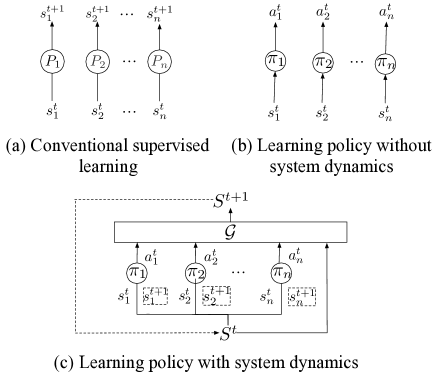
The modeling of human movements in space can be viewed as modeling the state transition of intelligent agents (e.g., human travelers, or vehicles with human drivers). The state of an agent can include its historical locations and its destination. Recently there are growing research studies that have developed computational methods to model the state transitions. One line of research directly predict the next states based on the current state and historical states (Song et al. 2016; Liu et al. 2016; Feng et al. 2017; Baumann et al. 2018; Feng et al. 2018; Gupta et al. 2018; Sadeghian, Kosaraju et al. 2019; Ma et al. 2019; Finn, Goodfellow, and Levine 2016; Oh et al. 2015). As is shown in Figure 1 (a), these methods focus on directly minimizing the error between estimated state $\hat{s}_{t+1}$ and true observed state $s_{t+1}$, with an end-to-end prediction model $P$ for the agent. In the real world where agents can take actions and interact with each other, the state of an agent is influenced not only by its previous states, but more importantly, by its action and the actions of other agents. It would require a large number of observed states that cover the whole state distribution to learn an accurate state transition model. When the agent encounters unobserved states, the learned model is likely to predict $s^{t+1}$ with a large error. An example is, when a vehicle drives on the road it has never observed before, these methods would fail to predict the movements. If we know the vehicle’s driving policy (e.g., the vehicle follows the shortest path to its destination), the vehicle’s movement can still be inferred.

Another line of research considers the underlying mechanism behind the state transition of agent movements from a decision-making perspective (Ziebart, Maas et al. 2018; Zou et al. 2018; Bhattacharyya et al. 2018; Song et al. 2018). As shown in Figure 1 (b), they aim to learn a decision policy $\pi$, which can generate the movements by taking a sequence of actions $a$ from policy model $\pi$. For example, imitation learning (IL) can be used to learn the routing policy of a vehicle, which aims to learn to take actions (e.g., keep moving on the current road, turn left, turn right, go straight, and take U-turn) based on the current state of the vehicle (e.g., the road ID, the number of vehicles and average speed on the road) (Ziebart, Maas et al. 2018). The learned policy is more applicable to the unobserved state because the dimension of action space is usually smaller than state space that increases exponentially with the number of state features. However, IL methods assume that the next state is purely decided by the action of the agent, while in the real world, the state transition of an agent is a combined effect of both agent decision and system dynamics. For example, if a driver presses the brake pedal, system dynamics determine this vehicle’s location after this action, which is mostly affected by factors such as the tires of vehicles, road surface, and weather. As another example, a person arrives at location $A$ and wants to check in, but $A$ has a limitation in the population it can serve. So the person would have to spend time waiting. Therefore, if we ignore the fact that the policy and final state of an agent must comply with the constraints from system dynamics, it will make the learned state transition model less realistic.

With the limitations of traditional prediction methods and imitation learning methods, in this paper, we formulate the problem of state transition modeling as modeling a decision-making process and incorporating system dynamics. Figure 1 (c) illustrates our formulation of the problem: in a system with $N$ agents, we consider the state of an agent as a joint outcome of its decision and system dynamics. At each timestep $t$, the agent observes state $s^{t}$ from the system state $S^{t}$, takes action $a^{t}$ following policy $\pi$ at every time step. Then the system model $\mathcal{G}$ considers current system state $S^{t}$ and the actions $\{a_{1}^{t},\cdots,a_{N}^{t}\}$ of all agents and outputs the next system state $S^{t+1}$, upon which the agents observe their next states $\{s_{1}^{t+1},\cdots,s_{N}^{t+1}\}$. This formulation looks into the mechanism behind state transitions and provides possibilities to include system dynamics in the modeling of state transitions.

In this paper, we propose MoveSD, which utilizes a similar framework as Generative Adversarial Imitation Learning (GAIL) (Ho and Ermon 2016) to model agents’ decision process, with a generator learning movement policy $\pi$ and a discriminator $\mathcal{D}$ learning to differentiate the generated movements from observed true movements. Moreover, MoveSD explicitly models system dynamics $\mathcal{G}$ and its influence on the state transition through learning $\pi$ and $\mathcal{D}$ with the constraints from $\mathcal{G}$ and through providing an additional intrinsic reward to $\pi$. Extensive experiments on real-world data demonstrate that our method can accurately predict the next state of an agent and accurately generate longer-term future states. In summary, our main contributions are:  
$\bullet$ We present the first attempt to learn to model the state transition of moving agents with system dynamics. Specifically, we formulate the state transition of human movements from the decision-making perspective and learn the movement policy under the framework of GAIL.  
$\bullet$ We show the necessity to consider the stochastic dynamics of the system when modeling state transitions and provide insights on different possible approaches to integrate the system dynamics.  
$\bullet$ We perform extensive experiments on real-world data, and the experimental results show that our method can generate similar human movement trajectories to the true trajectories, and has superior performances in applications like location prediction and trajectory generation compared with the state-of-the-art methods.

Preliminaries

In this section, we formulate our problem of modeling the state transition of human movements and then illustrate our definition using an example of a traveler moving in the grid world.

Figure 2: Illustration of the proposed framework. It has four main components: the system dynamics $\mathcal{G}_{\delta}$, the dynamic judger $J$, the agent policy $\pi_{\theta}$, and the discriminator $\mathcal{D}_{\psi}$. $\pi$ and $\mathcal{G}$ together influences the transition of states. The discriminator learns to differentiate between demonstrated trajectories and generated trajectories and provide reward $r_{D}$ for learning policy $\pi$ that behaves similarly to the true policy. The dynamics judger provides additional intrinsic reward $r_{J}$ from the system to the policy, indicating whether the policy behaves compliantly with system constraints $g$. Better viewed in color.

Definition 1 (State and action).

A state $s^{t}$ of an agent describes the surrounding environment of the agent at time $t$, and the action $a^{t}$ is the agent takes at time $t$ using its policy $\pi$, i.e., $a^{t}\sim\pi(a|s^{t})$.

Definition 2 (State trajectory and movement trajectory).

A state trajectory of an agent is a sequence of states generated by the agent, usually represented by a series of chronologically ordered pairs, i.e., $\mathcal{\xi}=(s^{t_{0}},\cdots,s^{t_{T}})$. A movement trajectory of an agent is a chronologically ordered sequence of state-action pairs, i.e., $\mathcal{\tau}=(\mathcal{\tau}^{t_{0}},\cdots,\mathcal{\tau}^{t_{T}})$ where $\mathcal{\tau}^{t_{i}}=(s^{t_{i}},a^{t_{i}})$ .

Problem 1.

Given a set of state trajectories $\mathcal{S}=\{\mathcal{\xi}_{1},\mathcal{\xi}_{2},\cdots,\mathcal{\xi}_{N}\}$ of a real-world system with $N$ agents, the overall objective is to learn the transition function $f(s^{t+1}|s^{t})$ from $s^{t}$ to $s^{t+1}$ so that the error between estimated state $\hat{s}^{t+1}$ and true state $s^{t+1}$ is minimized.

As in Figure 1 (a), traditional supervised learning solutions to this problem learn a direct mapping function $f_{\vartheta}$ from $s^{t}$ to $s^{t+1}$ through minimizing some loss function $\mathcal{L}$ over the set of state trajectories as training data: $\mathop{argmin}_{\vartheta}\mathbb{E}_{(s^{t},s^{t+1})\sim\mathcal{T}_{E}}[\mathcal{L}(s^{t+1},f_{\vartheta}(s^{t})]$.

In this paper, instead of learning a direct mapping from $s^{t}$ to $s^{t+1}$, we tackle the problem from a decision-making perspective. As shown in Figure 1 (c), in our problem, an agent observes state $s^{t}$ from the system state $S^{t}$, takes action $a$ following policy $\pi$ at every time step. System model $\mathcal{G}$ takes current system states $S^{t}$ and the actions $\{a_{1}^{t},\cdots,a_{N}^{t}\}$ as input, and decides the next system state $S^{t+1}$, upon which the agents observe their states $\{s_{1}^{t+1},\cdots,s_{N}^{t+1}\}$.

To better understand our definition, we use an example of learning to model traveler movements in a grid world, where the travelers move between grids, and there are several facilities scattered in the grids that the travelers might be interested.  
$\bullet$ State. In this example, the state $s$ of an agent includes the traveler’s information, e.g., coordinates of the current grid the traveler locates. State observations could also include the environment properties, e.g., the population in the current grid as well as events.  
$\bullet$ Action. The traveler’s action is its moving direction, which can mostly be inferred from its two consecutive locations. For example, if a traveler is at grid $A$ at time $t$ and its next location is $A$’s southwest neighboring grid, its action $a^{t}$ is “move southwest”.  
$\bullet$ Agent. Each traveler is an agent. A traveler takes action $a$ based on the current state $s^{t}$ according to his policy $\pi$, e.g., a traveler decides to move to the next location, keep wandering in the current location, or check-in at the facilities in current location based on his current state. The policy could vary for different agents, e.g., different travelers have different movement policies.  
$\bullet$ System dynamics. System dynamics $\mathcal{G}$ aggregates the current actions of all agents $\{s_{1}^{t},\cdots,s_{N}^{t}\}$ in the system, and influencing their next states $\{s_{1}^{t+1},\cdots,s_{N}^{t+1}\}$. For example, if a location has an event and has a queue in serving travelers, system dynamics determine the constraint $g_{i}$ like how long an upcoming traveler $i$ would wait to get served and influence the traveler’s next state. Note that $\mathcal{G}$ takes the system state $S$ as input, whereas the state $s$ of an agent is only part of the system state $S$ observed by the agent. The system dynamics model $\mathcal{G}$ is different from the agent policy $\pi$, where $\mathcal{G}$ reflects the physical transitions and constraints of the real world. In contrast, $\pi$ is the mapping from the agent’s observation to action.  
$\bullet$ Objective. This example’s objective is to minimize the difference between the observed traveler movement trajectories and the traveler trajectories generated by the learned transition model $f_{\theta,\delta}=\{\pi_{\theta},\mathcal{G}_{\delta}\}$, where $\pi$ and $\mathcal{G}$ are parameterized by $\theta$ and $\delta$.

Method

In this section, we first overview the general framework of MoveSD; then, we describe each component of the architectures; finally, we introduce the training process and discuss possible paradigms in learning the models.

Overview

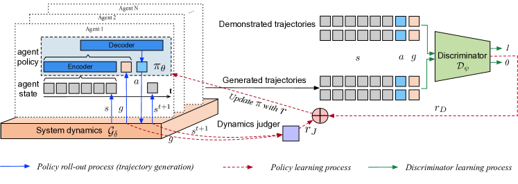
As is shown in Figure 2, MoveSD has four components, namely the system dynamics $\mathcal{G}_{\delta}$, the dynamic judger $J$, the agent policy $\pi_{\theta}$, and the discriminator $\mathcal{D}_{\psi}$ to model the state transition. We formulate the problem of learning the transition model $f_{\theta,\delta}=\{\pi_{\theta},\mathcal{G}_{\delta}\}$ to perform real-world-like movements by rewarding it for “deceiving” the discriminator $\mathcal{D}_{\psi}$ trained to discriminate between policy-generated and observed true trajectories.

The system dynamics $\mathcal{G}_{\delta}$ takes as input the system state $S$ and generates the physical constraints $g$ for each agent, which we parameterize as a multilayer perceptron (MLP). The policy $\pi_{\theta}$ takes as input the observed trajectories and the physical constraints $g^{t}$ from $\mathcal{G}_{\delta}$ and generate an action distribution $\pi_{\theta}(a|s)$ and sample an action $\hat{a}^{t}$ from the distribution, which we parameterize as a Recurrent Neural Network (RNN): $\hat{a}^{t}\sim\pi(a|s^{t-L},\cdots,s^{t};g^{t})$, where $L$ is the observed trajectory length.

The next state $s^{t+1}$ of the agent can be calculated based on $s^{t}$, $\hat{a}^{t}$ and with system states $S^{t}$. Then the movement trajectories $\mathcal{T}^{G}=\{\mathcal{\tau}_{1},\cdots,\mathcal{\tau}_{N}\}$ of $N$ agents in the system can be generated. The generated trajectories $\mathcal{T}^{G}$, are then fed to 1) the discriminator $\mathcal{D}_{\psi}$ to output a score of the probability of the trajectory being true and 2) the dynamics judger $\mathcal{J}$, a rule-based calculator, to measure the extent of state $s$ meeting system physical constraints $g$.

The policy $\pi_{\theta}$ and discriminator $\mathcal{D}_{\psi}$ are jointly optimized through the framework of GAIL (Ho and Ermon 2016) in the form of an adversarial minimax game as Generative Adversarial Network (GAN) (Goodfellow et al. 2014):

$$\mathop{max}_{\psi}\mathop{min}_{\theta}\mathcal{L}(\psi,\theta)=\mathbb{E}_{(s,a;g)\sim\mathcal{\tau}\in\mathcal{T}_{E}}\log\mathcal{D}_{\psi}(s,a;g)+$$ (1)

$$\mathbb{E}_{(s,a;g)\sim\mathcal{\tau}\in\mathcal{T}_{G}}\log(1-\mathcal{D}_{\psi}(s,a;g))-\beta H(\pi_{\theta})$$

where $\mathcal{T}_{E}$ and $\mathcal{T}_{G}$ are the observed true trajectories and the trajectories generated by $\pi_{\theta}$ and $\mathcal{G}_{\delta}$ in the system, $H(\pi_{\theta})$ is an entropy regularization term. Different from the vanilla GAIL whose discriminator is trained with $(s,a)$, in this paper, the discriminator is also conditioned on the system constraints as $\mathcal{D}_{\psi}(s,a;g)$.

Stochastic System Dynamics

System dynamics $\mathcal{G}$ can influence the movements of the agents in the form of system constraints $g$, including the temporal and the spatial constraints. The temporal constraint, i.e., the time for an agent to spend in a location, is particularly crucial in deciding the action of the agent. For example, due to the physical distance between two locations and the agent’s travel speed, it is unlikely for an agent to move arbitrarily from one location to another instantly. Another example is that the duration a traveler stays at a demanding location is influenced by the waiting time to get served. The spatial constraint, like obstacles that block the agent’s actions, is usually more stable than temporal constraints and can be learned with features like location ID. Therefore, in this work, we consider temporal constraint as the main influence of system dynamics underlying the agent decision-making process.

However, the stochasticity of system dynamics poses challenges to learn the system constraints since some factors in the system might be intrinsically unobserved and the system dynamics are naturally stochastic. For example, the duration of vehicles traveling on a specified road is dynamically changing with weather conditions or traffic signals, where we do not always observe the weather and traffic signal situation in the agent’s trajectory data.

To learn the stochastic constraints, instead of directly predicting a scalar value of the temporal constraint like traditional supervised learning methods do (Finn, Goodfellow, and Levine 2016; Oh et al. 2015; Song et al. 2010, 2016; Feng et al. 2018; Liu et al. 2016), we set out to learn the latent distribution of the temporal constraint.Since the temporal constraint $g$, i.e., the duration an agent stays in the location, is a real-valued scalar with lower and upper bounds (correspondingly 0 and maximum simulation steps in our cases), we can shift and rescale the values to be in the range $[0,1]$ and model $g$ as a sample from a Beta distribution $Beta(\Xi)$, where $\Xi=(\alpha,\beta)$ is the 2-dimensional shaping parameter for Beta distribution $(\alpha,\beta>0)$. Specifically, $\mathcal{G}$ is parameterized with an MLP:

$$h^{g}_{0}= \sigma(o_{g}W^{g}_{0}+b^{g}_{0}),h^{g}_{1}=\sigma(h^{g}_{0}W^{g}_{1}+b^{g}_{1}),\cdots$$ (2)

$$\Xi= \sigma(h^{g}_{G-1}W^{g}_{G}+b^{g}_{G}),g\sim Beta(\Xi)$$

where $G$ is the number of layers, $W^{g}_{i}\in\mathbb{R}^{n_{i-1}\times n_{i}}$, $b^{g}_{i}\in\mathbb{R}^{n_{i}}$ are the learnable weights for the $i$-th layer. $\sigma$ is ReLU function (same denotation for the following part of this paper), as suggested by (Radford, Metz, and Chintala 2015). For $i=0$, we have $W^{g}_{0}\in\mathbb{R}^{c\times n_{0}}$, $b^{g}_{0}\in\mathbb{R}^{n_{0}}$, where $c$ is the feature dimension for $o_{g}$ and $n_{0}$ is the output dimension for the first layer; for $i=G$, we have $W^{g}_{G}\in\mathbb{R}^{n_{G-1}\times 2}$, $b^{g}_{G}\in\mathbb{R}^{1\times 2}$.

Policy Network

The policy network consists of three major components: 1) observation embedding; 2) recurrent encoding; 3) action prediction.

Observation Embedding

We embed $k$-dimensional state features into an $m$-dimensional latent space via an embedding layer that copes with location ID $loc^{t}$, a layer of MLP for the rest of the state features $o^{t}$ and a concatenation layer on the outputs from previous two layers:

$$x^{t} =Concat(OneHot(loc^{t})W_{e},\sigma(o^{t}W_{o}+b_{o}))$$ (3)

where $W_{e}\in\mathbb{R}^{l\times m_{1}}$, $W_{o}\in\mathbb{R}^{k\times m_{2}}$ , $b_{o}\in\mathbb{R}^{m_{2}}$ are weight matrixes and bias vectors to learn. Here, there are total $l$ location IDs, and $m_{2}=m-m_{1}$. The concatenated state represents the current state of the agent.

Recurrent encoding

To reason about the status of the agent as well as the dynamic interactions between multiple agents, unlike conventional feed-forward neural policies (Ho and Ermon 2016; Li, Song, and Ermon 2017), we propose to learn the policy $\pi$ with an encoder-decoder model (Cho et al. 2014) to account for the sequential nature. To capture the individual status from its past observations, we input the observations of past $L_{in}$ timesteps to the encoder RNN, one observation per step, which progresses as: $h_{R}^{i}=RNN_{enc}(x^{i},h^{i-1}),\forall t-L_{in}\leq i\leq t$. The last hidden state, $h_{R}^{t}$ is the fixed-length descriptor of past trajectories for the agent.

Action prediction

The action prediction module takes the output of encoder RNN $h_{R}^{t}$, and the system dynamic constraints $g^{t}$ as input. The final action is sampled from the categorical distribution $p^{A}$ learned by an MLP:

$$h^{A}_{0} =Concat(h_{R}^{t},g^{t}),$$ (4)

$$h^{A}_{1} =\sigma(h^{A}_{0}W^{A}_{1}+b^{A}_{1}),\ h^{A}_{2}=\sigma(h^{A}_{1}W^{A}_{2}+b^{A}_{2}),\cdots$$

$$p^{A} =Softmax(h^{A}_{H-1}W^{A}_{H}+b^{A}_{H}),a^{t}\sim Cat(p^{A})$$

where $W^{A}_{i}\in\mathbb{R}^{d_{i-1}\times d_{i}}$, $b^{A}_{i}\in\mathbb{R}^{d_{i}}$ are the learnable weights for the $i$-th layer in action prediction module. For $i=H$, we have $W^{A}_{H}\in\mathbb{R}^{n_{H-1}\times|\mathcal{A}|}$, $b^{A}_{H}\in\mathbb{R}^{|\mathcal{A}|}$, where $|\mathcal{A}|$ is the total number of candidate actions.

Discriminator and Dynamics Judger

The discriminator network takes a similar network structure as a policy network, with the action prediction module in $\pi$ replaced by a binary classifier with an MLP. When training $\mathcal{D}_{\psi}$, Equation (1) can be set as a sigmoid cross entropy where positive samples are from observed true trajectories $\mathcal{T}_{E}$, and negative samples are from generated trajectories $\mathcal{T}_{G}$. Then optimizing $\psi$ can be easily done with gradient ascent on the following loss function:

$$\mathcal{L}_{D} =\mathbb{E}_{(s,a;g)\in\mathcal{T}_{E}}\log\mathcal{D}_{\psi}(s,a;g)$$ (5)

$$+\mathbb{E}_{(s,a;g)\in\mathcal{T}_{G}}\log(1-\mathcal{D}_{\psi}(s,a;g))$$

The transition between states in a real-world system is an integration of physical rules, control policies, and randomness, which means its true parameterization is assumed to be unknown. Therefore, given $\mathcal{T}_{G}$ generated by $\pi_{\theta}$ in the system, Equation (1) is non-differentiable w.r.t $\theta$ and the gradient cannot be directly back-propagated from $\mathcal{D}_{\psi}$ to $\pi_{\theta}$. Therefore, we learn $\pi_{\theta}$ through Trust Region Policy Optimization (TRPO) (Schulman et al. 2015) in reinforcement learning, with a surrogate reward function formulated from Equation (1) as:

$$r_{D}(s^{t},a^{t};g^{t})=-\log(1-\mathcal{D}_{\psi}(s^{t},a^{t};g^{t}))$$ (6)

Here, the surrogate reward $r_{D}(s^{t},a^{t},g^{t})$ is derived from the discriminator $\mathcal{D}_{\psi}$ and can be perceived to be useful in driving $\pi_{\theta}$ into regions of the state-action space at time $t$ similar to those in observations.

Dynamics judger $\mathcal{J}$

To avoid generating trajectories that do not meet the real-world constraints, it is necessary to provide guidance from system dynamics during the learning of policy $\pi_{\theta}$. To explicitly incorporate the system constraints, we draw inspiration from (Ding et al. 2019) and propose a novel intrinsic reward term into the learning of our policy as follows:

$$r_{J}(s^{t},a^{t},g^{t},s^{t+1})=\left\{\begin{aligned} &\ 0,\text{ $g^{t}>\Gamma(s^{t+1})$ or $a^{t}$ is not ``stay''}\\ &\ \frac{|g^{t}-\Gamma(s^{t+1})|}{g^{t}},\text{otherwise}\\ \end{aligned}\right.$$ (7)

where $\Gamma(s)$ is a pre-defined function that extracts the duration of the agent spent in the current location from state $s$, $g^{t}$ is the temporal constraint from system dynamics at time $t$. Intuitively, when $\Gamma(s^{t+1})\leq g^{t}$, $r_{J}$ should be positive if the agent takes $a^{t}$ of staying in the current location, indicating the agents should stay in the location to meet the constraint $g^{t}$. With such a design, the agent’s action will be rewarded when it meets the system constraints, and the generated movement is more likely to be a real-world movement.

The final surrogate reward for training $\pi_{\theta}$ is defined as follows:

$$r=(1-\eta)\cdot r_{J}(s^{t},a^{t},g^{t},s^{t+1})+\eta\cdot r_{D}(s^{t},a^{t},g^{t})$$ (8)

where $\eta$ is a hyper-parameter that balances the objective of satisfying the physical constraints and mimicking the true trajectories, both of which are pushing the policy learning towards modeling real-world transitions.

Training Process

The training procedure of MoveSD is an iterative process of learning policy $\pi_{\theta}$, discriminator $\mathcal{D}_{\psi}$ and system dynamics $\mathcal{G}_{\delta}$. We firstly initialize the parameters of $\mathcal{G}_{\delta}$, $\pi_{\theta}$ and $\mathcal{D}_{\psi}$ and pre-train $\mathcal{G}_{\delta}$. At each iteration of the algorithm, the policy parameters are used by every agent to generate trajectories $\mathcal{T}_{G}$. Rewards are then assigned to each state-action-goal pair in these generated trajectories. Then the generated trajectories are used to perform an update on the policy parameters $\theta_{i}$ via TRPO (Schulman et al. 2015) in reinforcement learning. Generated trajectories $\mathcal{T}_{G}$ and observed true trajectories $\mathcal{T}_{E}$ are subsequently used as the training data to optimize parameters $\psi$. Specifically, in learning $\mathcal{G}_{\delta}$, we use the observed trajectories of all agents and build training data for system dynamics $\mathcal{G}_{\delta}$ by extracting features $o_{g}$ for a location and calculating the duration that each agent spent in the location as labels $g$. In this paper, we use the location ID, time, the number of agents in the location as features, and predict constraints $g$ as the duration an agent stays in the location.

Experiment

Experimental Environments and Datasets

We evaluate our method in two real-world travel datasets: the travel behavior data in a theme park and the travel behavior of vehicles in a road network. The state and action definitions in each environment are shown in Table 1. The detailed statistics of the dataset can be found in the Appendix.  
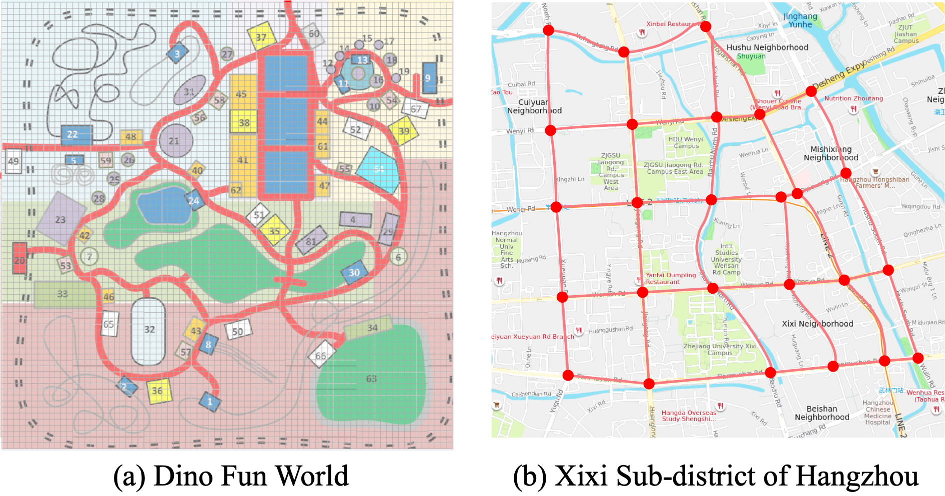
$\bullet$ ThemePark. This is an open-accessed dataset that contains the tracking information for all visitors to a theme park, DinoFun World, as is shown in Figure 3 (a). DinoFun World covers a geographic space of approximately 500x500 $m^{2}$ with ride attractions, and hosting thousands of visitors each day. All visitors must use a mobile application which records the location of visitors by a grid ID, where the whole park is divided into $5m\times 5m$ grid cells. Each data record contains a record time, a traveler ID, a grid ID, and an action. The action is recorded every second when travelers move from grid square to grid square or check-in at attractions.  
$\bullet$ RouteCity. This is a vehicle trajectory dataset captured from surveillance cameras installed around 25 intersections in Xixi Sub-district at Hangzhou, China, as is shown in Figure 3 (b). The trajectory of a recorded vehicle includes the timestamp, vehicle ID, road segment ID, and the action of the vehicle. The action can be staying on the current road segment, and transiting to the next road segment by turning left/right, taking U-turn, or going straight.

Table 1: State and action definition for travelers/vehicles in ThemePark and RouteCity. In ThemePark, travelers move between grids; the actions indicate which neighboring grid it travels or stay/check-in in the current grid. In RouteCity, vehicles move between road segments, and the actions indicate to stay in the current road or to go to different directions towards its neighboring roads.

Env	Type	Description
ThemePark	Time	Time spent in current grid, start time
	Location	Current grid ID, population in current grid, if current grid checkinable
	Action	Move to eight adjacent grids, stay or check-in in current grid
RouteCity	Time	Time spent in current road, start time
	Location	Current road ID, destinated road, current population in the grid, previous road
	Activity	Last action
	Action	Turn left, turn right, take u-turn, go straight, stay on current road

Figure 3: Experiment environments in this paper. Left: Map of Dino Fun World in ThemePark. Right: Xixi Sub-district of Hangzhou, China in RouteCity.

Figure 4: Performance of different methods, including state-of-the-art baselines and the variants of our proposed model. (a) The accuracy (Acc@N) of predicting the next location. The higher, the better. (b) The average displacement error (ADE) and final displacement error (FDE) of generating future trajectories. The lower, the better. MoveSD performs the best against state-of-the-art baselines and its variants. Best viewed in color.

Baselines

We compare with both classical and state-of-the-art methods in human mobility prediction and imitation learning algorithms. We use the same features in deep learning-based methods and our proposed method for a fair comparison.  
$\bullet$ Random Walk (Brockmann, Hufnagel, and Geisel 2006). This is a classic method that models the movement of agents as a stochastic process, where the agent takes action among all possible actions with equal probability.  
$\bullet$ Markov Model (Gambs, Killijian, and del Prado Cortez 2012). The Markov-based method regards all the visited locations as states and builds a transition matrix to capture the first or higher-order transition probabilities between them. Following existing methods (Feng et al. 2018; Gao et al. 2019), we use the first-order Markov model in our experiment.  
$\bullet$ RNN Model is widely used to predict the next location by modeling temporal and spatial history movements (Liu et al. 2016; Gao et al. 2019; Feng et al. 2018). In this paper, we use LSTM in (Liu et al. 2016) as the base network of our proposed model and as a baseline.  
$\bullet$ GAN Model (Sadeghian, Kosaraju et al. 2019) uses the framework of generative adversarial networks to generate the next location based on past states without explicitly modeling the agent’s actions (Gupta et al. 2018; Sadeghian, Kosaraju et al. 2019; Ma et al. 2019; Feng et al. 2020).  
$\bullet$ GAIL considers the actions of the agents explicitly by learning the decision policy with generative adversarial networks (Ho and Ermon 2016; Song et al. 2018; Zheng, Liu et al. 2020; Wei et al. 2020). Different from our proposed model, GAIL uses feed-forward networks without the system dynamics.

Tasks and Metrics

To measure the discrepancy between the learned state transition model and real-world transitions, we evaluate the performance of different methods in the following two tasks:

Next location prediction. Given the same input states for an agent, a good state transition model should perform well in predicting the next location. Following existing studies (Song et al. 2010, 2016; Feng et al. 2018), we use the standard evaluation performance metrics, Acc@k, which ranks the candidate next locations by the probabilities generated from the model, and check whether the ground-truth location appears in the top $k$ candidate locations.

Trajectory generation. Given the same initial states for an agent, a good state transition model should not only perform well in predicting the next location but also be precise in generating the future trajectories as observed ones. Therefore, we also evaluate the performance on generating trajectory to measure the discrepancy between the learned transition model and real transitions, with the following metrics widely used in existing literature (Zou et al. 2018; Lisotto, Coscia, and Ballan 2019; Liang et al. 2019):   
$\bullet$ Average Displacement Error (ADE): The average of the root mean squared error (RMSE) between the ground truth coordinates $Y_{i}^{t}$ and the predicted coordinates:$\hat{Y}_{i}^{t}$ at every timestamp $t$ for every trajectory $i$: $ADE=\frac{\sum_{i=1}^{N}\sum_{t=1}^{T_{pred}}\sqrt{(\hat{Y}^{t}_{i}-Y^{t}_{i})^{2}}}{N\cdot T_{pred}}$   
$\bullet$ Final Displacement Error (FDE): The average of the RMSE at the final predicted points $\hat{Y_{i}}$ and the final true points $Y_{i}$ of all trajectories: $FDE=\frac{\sum_{i=1}^{N}\sqrt{(\hat{Y}_{i}-Y_{i})^{2}}}{N}$

Experimental Settings

We specify some of the important parameters here and all the parameter settings can be found in our codes. In all the following experiments, if not specified, the observed time length $L_{in}$ is set to be 10. The output length of $L_{out}$ is 1 for the next location prediction task, and 1000 for trajectory generation task. We fix the length $L_{in}$ and $L_{out}$ for simplicity, but our methods can be easily extended to different lengths since the neural networks are recurrent in taking the trajectories as input and in predicting future trajectories. We sample the trajectories at every second for ThemePark, and at every 10 seconds for RouteCity. $\eta$ is set as 0.8.

Overall Performance

In this section, we investigate the performance of our proposed method MoveSD on learning the travel movements in two real-world datasets from two perspectives: predicting the next location and generating future trajectories. Figure 3 shows the performance of the proposed MoveSD, classic models as well as state-of-the-art learning methods in the real-world environments. We have the following observations:  
$\bullet$ MoveSD achieves consistent performance improvements over state-of-the-art prediction and generation methods (RNN Model and GAN Model respectively) across different environments. The performance improvements are attributed to the benefits from the modeling of the decision process with GAIL and the integration with system dynamics. We also noticed that GAIL achieves better performance than GAN Model in most cases. This is because GAIL explicitly model the movement policy of agents, which conveys the importance of modeling the decision-making process in human movement.  
$\bullet$ The performance gap between the proposed MoveSD and baseline methods becomes larger in trajectory generation than in the next location prediction. This is because the framework of GAIL, which iteratively updates policy $\pi_{\theta}$ and discriminator $\mathcal{D}_{\psi}$ enables us to model the decision process that determines the whole trajectory effectively. The discriminator in our model can differentiate whether the trajectory is generated or real, which can drive the bad-behaved actions in one iteration to well-behaved ones during the policy learning process of the next iteration.

Ablation study

In this section, we perform an ablation study to measure the importance of learning the decision-making policy and the system dynamics.  
$\bullet$ MoveSD wo/ GAIL. This model takes both the state and constraints from system dynamics as its input and output the next location directly, which does not learn the movement policy in the decision-making process of the agent. It can also be seen as RNN Model methods with the information of system dynamics.  
$\bullet$ MoveSD wo/ dynamic. This method uses GAIL but does not consider the system dynamics. That is, the input of the policy and discriminator do not contain $g$ from system dynamic model $\mathcal{G}$.  
$\bullet$ MoveSD. This is our final method, which uses the adversarial learning process as GAIL, and considers the system dynamic.

Figure 4 shows the performance of variants of our method.We have the following observations:  
$\bullet$ MoveSD outperforms both MoveSD wo/ dynamic and MoveSD wo/ GAIL, indicating the effectiveness of using GAIL and the system dynamics. Compared with MoveSD wo/ GAIL, MoveSD performs better because it learns the decision-making process as the underlying mechanism behind the movements. Compared with MoveSD wo/ dynamic, MoveSD takes the system constraint $g$ into consideration, learning movement policies to avoid those infeasible actions that do not comply with the system dynamics.  
$\bullet$ We also notice that MoveSD wo/ GAIL outperforms pure RNN Model in most cases. This is because MoveSD wo/ GAIL has extra information on the constraints from system dynamics within the model, which validates the effectiveness of considering system dynamics. In the rest of our experiments, we only compare MoveSD with other methods.

To get deeper insights on MoveSD, we also investigated the following aspects about our model and their empirical results are left in the appendix due to page limits: (1) different paradigms in training $\mathcal{G}$, (2) the necessity of stochastic modeling of $\mathcal{G}$ and (3) sensitivity study. We also provided a case study for better understanding.

Conclusion

In this paper, we present a novel perspective in modeling the state transition of human movement in space as a decision process and learns the decision making policy with system dynamics. Specifically, we argue it is important to integrate the constraints from the system dynamic to help the learned state transition more realistic. Extensive experiments on real-world data demonstrate that our method can not only accurately predict the next state of agents, but also accurately generate longer-term future movements.

While MoveSD substantially provides insights to model human movements from decision making perspective with system constraints, we believe that this problem merits further study. One limitation of our current method is that, we model the human movements over discrete action space, whereas the movement of human over free space is continuous. An exciting direction for future work would be to develop stronger learning models for continuous action space. Second, the raw data for observation only include the status of travelers or vehicles and the location information. More exterior data like weather conditions might help to boost model performance. Lastly, we can further model different modalities in policies for different kinds of agents like private cars and taxis.

Appendix

A. Dataset Description

In this paper, we use two real-world human movement datasets:

ThemePark: This is an open-accessed dataset that contains the tracking information for all of the paying park visitors to a simulated park, DinoFun World. DinoFun World covers a large geographic space (approx. 500x500 $m^{2}$) and is populated with ride attractions, restaurants, and food stops, and hosting thousands of visitors each day. All visitors to the park use a parking app to check into rides and some other attractions. The park is equipped with sensor beacons that record movements within the park. Sensors are sensitive within a $5m\times 5m$ grid cell. Each data record contains a record time, a traveler ID, a grid ID with coordinate locations, and an action. The action is recorded every second when travelers move from grid square to grid square or “check-in” at rides, meaning they either get in line or onto the ride.

RouteCity. This is a trajectory dataset of vehicles captured from surveillance cameras installed around 25 intersections in Xixi Sub-district at Hangzhou, China. Each data record consists of a record time, a vehicle ID, an intersection ID. By analyzing these records with camera locations, the trajectory of a vehicle can be recovered as a timestamp, a vehicle ID, a road segment ID, and an action of the vehicle. The actions can be inferred from the consecutive road segments at every 10 seconds. The vehicles have actions like keeping traveling on the current road segment or transiting to the next road segment by turning left, turning right, taking U-turn, or going straight.

B. Model Parameters and Configurations

The hyper-parameters for our network structure and training process is shown in Table 2.

Table 2: Parameter settings

Parameter	Value	Parameter	Value
Number of hidden layers $G$ in $\mathcal{G}$	2	Feature length $n$ of hidden layers in $\mathcal{G}$	50
Input feature dimension $c$	3	Output dimension	2
Number of recurrent units	10	Embedding size $m_{1}$	50
Number of hidden layers $H$ in Recurrent module	2	Feature length $d$ of hidden layers for MLPs	50
Activation function of hidden layers	ReLU	Activation function of output layer in $\pi$	Softmax
Activation function of output layer in$\mathcal{G}$	ReLU	Activation function of output layer in $\mathcal{D}$	Sigmoid
Vocabulary size in embedding $l$		10000 in ThemePark, 78 in RouteCity
State feature dimension $k$		6 in ThemePark, 12 in RouteCity
Number of actions $|\mathcal{A}|$		11 in ThemePark, 5 in RouteCity
Total training iterations for generator and discriminator update		100
Batch size	128	Learning rate	0.0003
Discount factor $\gamma$ for TRPO	0.8	Gradient clip threshold for TRPO	0.2
$\lambda$ of Advantage Estimator for TRPO	0.98	Maximum iterations for GAIL	100
$\mathcal{D}$ updating frequency per iteration	5	$\pi$ updating frequency per iteration	100

C. Model update for Beta Distribution in $\mathcal{G}$

When the targets in $\mathcal{G}$ are real-valued scalars with lower and upper bounds, we can shift and rescale the values to be in the range [0, 1] and model the target as a sample from a Beta distribution. It can be parameterized by a neural network that outputs two values $\alpha,\beta>0$. The relationships between the temporal constraint $g$ and the shaping parameters $\alpha,\beta$ are as follows:

$$p_{\alpha,\beta}(g)=g^{\alpha-1}(1-g)^{\beta-1}\frac{\Gamma(\alpha\beta)}{\Gamma(\alpha)\Gamma(\beta)}$$ (9)

with log-likelihood:

$$ln\ p_{\alpha,\beta}(g) =(\alpha-1)ln(g)+(\beta-1)ln(1-g)$$ (10)

$$+ln\ \Gamma(\alpha\beta)-ln\ \Gamma(\alpha)-ln\ \Gamma(\beta)$$

and gradients:

$$\frac{\partial}{\partial\alpha}ln(p_{\alpha,\beta}(g))=ln(g)+\Psi(\alpha\beta)-\Psi(\alpha)$$ (11)

$$\frac{\partial}{\partial\beta}ln(p_{\alpha,\beta}(g))=ln(1-g)+\Psi(\alpha\beta)-\Psi(\beta)$$

where $\Psi$ is the digamma function $\Psi(x)=\frac{\partial}{\partial x}ln(\Gamma(x))$.

1

Input: Observed true trajectories $\mathcal{T}_{E}$, initial system dynamics, policy and discriminator parameters $\delta_{0}$, $\theta_{0}$, $\psi_{0}$, training option

Output: Policy $\pi_{\theta}$, Discriminator $\mathcal{D}_{\psi}$, System dynamics $\mathcal{G}_{\delta}$

2

3if Option 1 then

4       $\bullet$ Pretrain system dynamics $\mathcal{G}_{\delta}$ using Eq. (11)

5 end if

6for i $\longleftarrow$ 0, 1, … do

7       $\bullet$ Rollout trajectories for all agents $\mathcal{T}_{G}=\{\mathcal{\tau}|\mathcal{\tau}=(\mathcal{\tau}^{t_{0}},\cdots,\mathcal{\tau}^{t_{T}})\}$, where $\mathcal{\tau}^{t}=(s^{t},a^{t},g^{t},s^{t+1})$, $g^{t}=\mathcal{G}_{\delta}(o^{t}_{g})$, and $a^{t}\sim\pi_{\theta_{i}}(s^{t},a^{t},g^{t})$;

8      

9      # Generator update step

10      

11      $\bullet$ Score $\mathcal{\tau}^{t}$ from $\mathcal{T}^{D}_{G}$ with discriminator, generating reward using Eq. (6);

12      

13      if Option 2 then

14             $\bullet$ Update system dynamics $\mathcal{G}_{\delta}$;

15             $\bullet$ Update $\theta$ given $\mathcal{T}^{D}_{G}$ by optimizing Eq. (1);

16            

17       end if

18      else if Option 3 then

19             $\bullet$ Update $\theta$ and $\delta$ given $\mathcal{T}^{D}_{G}$ by optimizing Eq. (1) and using Eq. (11);

20            

21       end if

22      else

23             $\bullet$ Update $\theta$ given $\mathcal{T}^{D}_{G}$ by optimizing Eq. (1);

24            

25       end if

26      # Discriminator update step;

27       $\bullet$ Update $\psi$ by optimizing Eq. (5);

28      

29 end for

Algorithm 1 Training procedure of MoveSD with options

D. Detailed algorithms for different options in training paradigms

Since the system constraint $g$ given by $\mathcal{G}_{\delta}$ is used in $\mathcal{\tau}$ when learning $\pi_{\theta}$ and $\mathcal{D}_{\psi}$, here we discuss the options in learning $\mathcal{G}_{\delta}$, and investigate their effectiveness empirically in Appendix D-2.  
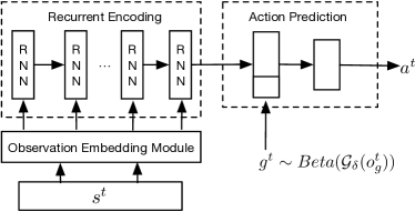
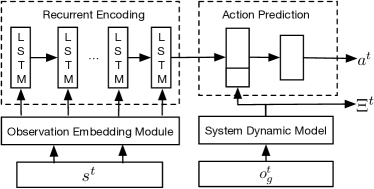
$\bullet$ Option 1 (Default): Pre-train $\mathcal{G}_{\delta}$ before the learning of $\pi_{\theta}$ and $\mathcal{D}_{\psi}$ (line 1 in Algorithm 1), fix $\delta$ during the learning of $\theta$ and $\psi$. The architecture for this network is shown in Figure 5  
$\bullet$ Option 2: At each round of updating $\pi_{\theta}$ and $\mathcal{D}_{\psi}$, we update $\mathcal{G}_{\delta}$ as well based on the generated trajectories.  
$\bullet$ Option 3: Integrate the $\mathcal{G}_{\delta}$ with $\pi_{\theta}$ in one model, as is shown in Figure 5(b). The output of $\mathcal{G}_{\delta}$ is fed into $\pi$ before action prediction module. The training of this option would require a model that is optimized through multi-task learning, with one task learns the action prediction and the other task learns to predict $g$.

Their training algorithm is shown in Algorithm 1.

(a) Option 1 & 2	(b) Option 3

Figure 5: Different architectures of policy network

E. Additional Experiments

1. Stochastic/Deterministic modeling of $\mathcal{G}$

As mentioned in Section Stochastic System Dynamics, we model the system constraint from $\mathcal{G}$ by modeling the distribution to mimic the stochastic nature of system dynamics. In this section, we investigate whether this stochastic modeling is necessarily by comparing it with deterministic modeling, which directly output a scalar value.

As is shown in Table 3, MoveSD with stochastic $\mathcal{G}$ achieves consistently better performance than deterministic $\mathcal{G}$. The reason is that there are unobserved factors and stochastic $\mathcal{G}$ learns the distribution of data with probability, which can be used to learn with this kind of missing data. In the rest of the experiments, we only use stochastic $\mathcal{G}$ in MoveSD and compare it with other baseline methods.

2. Different training paradigms of $\mathcal{G}$

As mentioned in Section Training Process, $\pi$ can be trained in different ways with regards to $\mathcal{G}$: 1) pre-trained $\mathcal{G}$, 2) $\mathcal{G}$ iteratively trained with $\pi$, or 3) $\mathcal{G}$ jointly learned with $\pi$ in one model.

The results in Table 3 show that MoveSD with pre-training $\mathcal{G}$ achieves similar performance with using one model integrating both $\mathcal{G}$ and $\pi$, but outperforms training $\mathcal{G}$ and $\pi$ iteratively. The reason could be that if the errors for predicting $g$ form $\mathcal{G}$ is large in the current iteration and if the errors cannot propagate back to the learning of $\pi$, $\pi$ taking $g$ from $\mathcal{G}$ would lead to further error. Therefore, a good start of $\mathcal{G}$ through pre-training or using one model to learn both $\mathcal{G}$ and $\pi$ can lead to relatively better performance. In the rest of the experiments, we only use pre-trained $\mathcal{G}$ in MoveSD and compare it with other baseline methods.

(a) Accuracy of location prediction in ThemePark and RouteCity		(b) Error of trajectory generation in ThemePark and RouteCity

Figure 6: Performance of MoveSD under with different base models, compared with RNN Model (LSTM). (a) Accuracy of next location prediction under both scenarios. The higher, the better. (b) Error of trajectory generation under both scenarios. The lower, the better. MoveSD consistently outperforms RNN Model. Best viewed in color.

(a) ThemePark	(b) RouteCity

Figure 7: Performance of MoveSD for trajectory generation with different values of $\eta$. The lower, the better.

Figure 8: A case study on a vehicle’s movement in the first 1000 seconds. All the methods take the same initial information that the vehicle starts its movement at location $A$ at the 320 second, and its destination is location $B$ (shown as the red star). The numbers next to the nodes are the time of vehicles arriving at corresponding intersections. The blue lines are the true observed trajectories of the vehicle, where it only reaches $C$ at the 1000 second. The red lines in different figures indicate the trajectories generated by different methods. Only MoveSD can generate a similar trajectory as observed. Best viewed in color.

Table 3: Investigation of stochastic/deterministic modeling of $\mathcal{G}$ and different training paradigms for $\pi$ and $\mathcal{G}$ in generating trajectories. The lower, the better. Stochastic modeling is better than deterministic modeling. Pre-training $\mathcal{G}$ and jointly learning $\mathcal{G}$ with $\pi$ achieves slightly better performance than iteratively updating $\mathcal{G}$ and $\pi$.

	Options	ThemePark		RouteCity
		ADE(m)	FDE(m)	ADE(km)	FDE(km)
Deter- ministic	#1: Pre-trained $\mathcal{G}$	15.653	22.231	0.236	0.498
	#2: Iterative training	17.829	25.932	0.270	0.531
	#3: One model	14.325	22.617	0.242	0.515
Stoch- astic	#1: Pre-trained $\mathcal{G}$	9.842	16.716	0.154	0.301
	#2: Iterative training	13.122	20.970	0.189	0.343
	#3: One model	10.399	17.806	0.160	0.292

3. Sensitivity Study: different base models in $\pi$

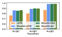
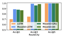
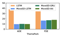
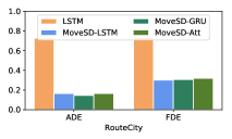
In this section, we investigate the impact of base RNN models in $\pi$ proposed in the existing literature - more specifically, GRU as in (Gao et al. 2019), attentional RNN as in (Feng et al. 2018), and LSTM (Liu et al. 2016), termed MoveSD-GRU, MoveSD-Att, and MoveSD-LSTM respectively. Figure 6 summarizes the experimental results. We have the following observations:  
$\bullet$ Our proposed method performs steadily under different base models across various tasks, indicating the idea of our method is valid across different base models. In the rest of our experiments, we use LSTM as our base model and compare it with other baseline methods.  
$\bullet$ Our proposed method with different base models performs consistently better than the baseline method RNN Model. This is because our method not only learns to model the behavior but also considers the influence of system dynamics.

4. Sensitivity Study: different values of balancing parameter $\eta$

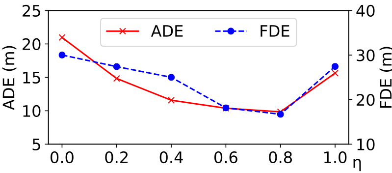
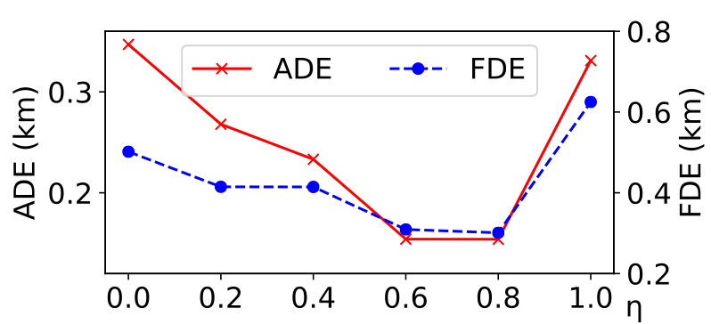
In this section, we study the influence of $\eta$ in Equation (8), which balances the reward from the discriminator $\mathcal{D}_{\psi}$ and the dynamics judger $\mathcal{J}$. As is shown in Figure 7, when we use a combined reward from both $\mathcal{J}$ and $\mathcal{D}_{\psi}$, MoveSD performs better than purely from $\mathcal{J}$ $(\eta=0)$ and purely from $\mathcal{D}_{\psi}$ $(\eta=1)$. In this paper, we set $\eta$ as 0.8 as it performs the best empirically.

F. Case Study

In this section, we showcase the trajectory of a vehicle generated by different methods under RouteCity, as is shown in Figure 8. Blue lines are the true observed trajectories of the vehicle, where we can see the observed vehicle starts traveling at the 320 seconds, passing through two road segments toward its destination (red star) and only reaches at $C$ at the 1000 second. It spends a certain time on each road, due to the physical length of roads and the travel speed on the road. The red lines indicate the trajectory generated by different methods. We can see that only MoveSD can generate a similar trajectory as observed, while all other baselines generate unrealistic trajectories. Specifically, since RNN Model yields inaccurate predictions when encountering a new state and the generated trajectory drifts away eventually because of the accumulated inaccuracy in previous predictions. On the other hand, MoveSD explicitly models the mechanism behind state transitions and learns to generate trajectories with physical constraints.

G. Detailed results for Figure 4

Table 4 shows the numerical results of Figure 4. MoveSD performs the best against state-of-the-art baselines and its variants.

Table 4: Performance of different methods in predicting the next location and generating future trajectories w.r.t accuracy (Acc@N), average displacement error (ADE), and final displacement error (FDE). For Acc@N, the higher, the better; for ADE and FDE, the lower, the better. MoveSD performs the best against state-of-the-art baselines and its variants.

	ThemePark					RouteCity
	Predicting next location			Generating 1000 steps		Predicting next location			Generating 1000 steps
	Acc@1	Acc@3	Acc@5	ADE(m)	FDE(m)	Acc@1	Acc@3	Acc@5	ADE(km)	FDE(km)
Random Walk	0.120	0.358	0.574	67.291	75.492	0.192	0.573	1.000 ∗	1.589	1.644
Markov Model	0.734	0.788	0.795	45.087	39.768	0.408	0.539	1.000	1.105	1.149
RNN Model	0.767	0.806	0.871	38.129	34.196	0.704	0.752	1.000	0.727	0.733
GAN Model	0.759	0.812	0.925	30.861	32.689	0.701	0.700	1.000	0.723	0.757
GAIL	0.766	0.810	0.938	20.928	28.222	0.664	0.771	1.000	0.501	0.752
MoveSD wo/ dynamic	0.771	0.853	0.979	15.634	27.454	0.726	0.959	1.000	0.331	0.625
MoveSD wo/ GAIL	0.756	0.847	0.906	21.602	28.762	0.759	0.783	1.000	0.724	0.724
MoveSD	0.864	0.892	0.986	9.842	16.716	0.892	0.994	1.000	0.154	0.301

^∗Acc@5 in RouteCity are all equals to 1 because the maximum number of next candidate locations is 5.

References

- Baumann et al. (2018) Baumann, P.; Koehler, C.; Dey, A. K.; and Santini, S. 2018. Selecting individual and population models for predicting human mobility. IEEE Transactions on Mobile Computing 17(10): 2408–2422.
- Bhattacharyya et al. (2018) Bhattacharyya, R. P.; Phillips, D. J.; Wulfe, B.; Morton, J.; Kuefler, A.; and Kochenderfer, M. J. 2018. Multi-agent imitation learning for driving simulation. In IROS’18.
- Brockmann, Hufnagel, and Geisel (2006) Brockmann, D.; Hufnagel, L.; and Geisel, T. 2006. The scaling laws of human travel. Nature 439(7075): 462–465.
- Cho et al. (2014) Cho, K.; Van Merriënboer, B.; Gulcehre, C.; Bahdanau, D.; et al. 2014. Learning phrase representations using RNN encoder-decoder for statistical machine translation. arXiv preprint arXiv:1406.1078 .
- Ding et al. (2019) Ding, Y.; Florensa, C.; Abbeel, P.; and Phielipp, M. 2019. Goal-conditioned imitation learning. In NIPS’19.
- Dulac-Arnold, Mankowitz, and Hester (2019) Dulac-Arnold, G.; Mankowitz, D.; and Hester, T. 2019. Challenges of real-world reinforcement learning. arXiv preprint arXiv:1904.12901 .
- Feng et al. (2018) Feng, J.; Li, Y.; Zhang, C.; Sun, F.; Meng, F.; Guo, A.; and Jin, D. 2018. Deepmove: Predicting human mobility with attentional recurrent networks. In The World Wide Web Conference.
- Feng et al. (2020) Feng, J.; Yang, Z.; Xu, F.; et al. 2020. Learning to Simulate Human Mobility. In KDD’20.
- Feng et al. (2017) Feng, S.; Cong, G.; An, B.; and Chee, Y. M. 2017. Poi2vec: Geographical latent representation for predicting future visitors. In AAAI’17.
- Finn, Goodfellow, and Levine (2016) Finn, C.; Goodfellow, I.; and Levine, S. 2016. Unsupervised learning for physical interaction through video prediction. In NIPS’16.
- Gambs, Killijian, and del Prado Cortez (2012) Gambs, S.; Killijian, M.-O.; and del Prado Cortez, M. N. 2012. Next place prediction using mobility markov chains. In Proceedings of the First Workshop on Measurement, Privacy, and Mobility, 1–6.
- Gao et al. (2019) Gao, Q.; Zhou, F.; Trajcevski, G.; Zhang, K.; Zhong, T.; and Zhang, F. 2019. Predicting human mobility via variational attention. In The World Wide Web Conference.
- Goodfellow et al. (2014) Goodfellow, I.; Pouget-Abadie, J.; Mirza, M.; Xu, B.; Warde-Farley, D.; Ozair, S.; Courville, A.; and Bengio, Y. 2014. Generative adversarial nets. In NIPS’14.
- Gupta et al. (2018) Gupta, A.; Johnson, J.; Fei-Fei, L.; Savarese, S.; and Alahi, A. 2018. Social GAN: Socially acceptable trajectories with generative adversarial networks. In CVPR’18.
- Ho and Ermon (2016) Ho, J.; and Ermon, S. 2016. Generative adversarial imitation learning. In NIPS’16.
- Li, Song, and Ermon (2017) Li, Y.; Song, J.; and Ermon, S. 2017. Inferring the latent structure of human decision-making from raw visual inputs. arXiv preprint arXiv:1703.08840 2.
- Lian et al. (2014) Lian, D.; Zhao, C.; Xie, X.; et al. 2014. GeoMF: joint geographical modeling and matrix factorization for point-of-interest recommendation. In KDD’14.
- Liang et al. (2019) Liang, J.; Jiang, L.; Niebles, J. C.; Hauptmann, A. G.; and Fei-Fei, L. 2019. Peeking into the future: Predicting future person activities and locations in videos. In CVPR’19.
- Lisotto, Coscia, and Ballan (2019) Lisotto, M.; Coscia, P.; and Ballan, L. 2019. Social and Scene-Aware Trajectory Prediction in Crowded Spaces. In CVPR’19.
- Liu et al. (2016) Liu, Q.; Wu, S.; Wang, L.; and Tan, T. 2016. Predicting the next location: A recurrent model with spatial and temporal contexts. In AAAI’16.
- Ma et al. (2019) Ma, Y.; Zhu, X.; Zhang, S.; Yang, R.; Wang, W.; and Manocha, D. 2019. Trafficpredict: Trajectory prediction for heterogeneous traffic-agents. In AAAI’19.
- Oh et al. (2015) Oh, J.; Guo, X.; Lee, H.; Lewis, R. L.; and Singh, S. 2015. Action-conditional video prediction using deep networks in atari games. In NeurIPS’15.
- Radford, Metz, and Chintala (2015) Radford, A.; Metz, L.; and Chintala, S. 2015. Unsupervised representation learning with deep convolutional generative adversarial networks. arXiv:1511.06434 .
- Sadeghian, Kosaraju et al. (2019) Sadeghian, A.; Kosaraju, V.; et al. 2019. Sophie: An attentive GAN for predicting paths compliant to social and physical constraints. In CVPR’19.
- Schulman et al. (2015) Schulman, J.; Levine, S.; Abbeel, P.; Jordan, M.; and Moritz, P. 2015. Trust Region Policy Optimization. In ICML’15.
- Song et al. (2010) Song, C.; Qu, Z.; Blumm, N.; and Barabási, A.-L. 2010. Limits of predictability in human mobility. Science 327(5968): 1018–1021.
- Song et al. (2018) Song, J.; Ren, H.; Sadigh, D.; and Ermon, S. 2018. Multi-agent generative adversarial imitation learning. In NIPS’18.
- Song et al. (2016) Song, X.; Zhang, Q.; Sekimoto, Y.; Shibasaki, R.; Yuan, N. J.; and Xie, X. 2016. Prediction and simulation of human mobility following natural disasters. ACM Transactions on Intelligent Systems and Technology (TIST) 8(2): 1–23.
- Wang et al. (2017) Wang, J.; Chen, C.; Wu, J.; and Xiong, Z. 2017. No longer sleeping with a bomb: a duet system for protecting urban safety from dangerous goods. In KDD’17.
- Wang, Wang, and Wu (2018) Wang, J.; Wang, X.; and Wu, J. 2018. Inferring metapopulation propagation network for intra-city epidemic control and prevention. In KDD’18.
- Wei et al. (2020) Wei, H.; Chen, C.; Liu, C.; Zheng, G.; and Li, Z. 2020. Learning to Simulate on Sparse Trajectory Data. ECML-PKDD’20 .
- Wei et al. (2018) Wei, H.; Zheng, G.; Yao, H.; and Li, Z. 2018. Intellilight: A reinforcement learning approach for intelligent traffic light control. In KDD’18.
- Wu, Bayen, and Mehta (2018) Wu, C.; Bayen, A. M.; and Mehta, A. 2018. Stabilizing traffic with autonomous vehicles. In ICRA’18.
- Zheng, Liu et al. (2020) Zheng, G.; Liu, H.; et al. 2020. Learning to Simulate Vehicle Trajectories from Demonstrations. In ICDE’20.
- Ziebart, Maas et al. (2018) Ziebart, B. D.; Maas, A. L.; et al. 2018. Maximum entropy inverse reinforcement learning. In AAAI’18.
- Zou et al. (2018) Zou, H.; Su, H.; Song, S.; and Zhu, J. 2018. Understanding human behaviors in crowds by imitating the decision-making process. In AAAI’18.