Bulk odd-frequency pairing in the superconducting Su-Schrieffer-Heeger model

Abstract

The Su-Schrieffer-Heeger model describes fermions that hop on a one-dimensional chain with staggered hopping amplitude, where the unit cell contains two sites, or two sublattices. In this work we consider the Su-Schrieffer-Heeger model with superconducting pairing and show that the sublattice index acts as an additional quantum number in the classification of Cooper pairs, giving rise to inter- and intra-sublattice odd-frequency pair correlations in the bulk. Interestingly, this system behaves as a two band superconductor where the bulk odd-frequency correlations depend solely on the intrinsic staggering properties of the model. In general, odd-frequency correlations coexist with even-frequency correlations in both the trivial and topological phases, with comparable and even larger odd-frequency amplitudes at the topological phase transition points at low frequencies, due to the closing of the energy gap at these points. Furthermore, we also discuss how bulk odd-frequency amplitudes are correlated with pseudo-gaps in the density of states and also with a charge density wave that appears due to the chemical potential imbalance between sublattices.

I Introduction

Superconducting properties are highly determined by the symmetry of the Cooper pair wave function, or pair amplitude. Due to the fermionic nature of electrons, Fermi-Dirac statistics imposes antisymmetry on the pair amplitude under the total exchange of all quantum numbers, which can include spin, orbital, band, spatial and time coordinates, etc. The antisymmetry condition allows for electrons to pair at equal times but, interestingly, also permits pairing at different times, giving rise to temporally non-local pair amplitudes, which can be odd under the exchange of time coordinates, or equivalently odd in frequency ($\omega$).Berezinskii (1974); Bergeret et al. (2005); Tanaka et al. (2012); Linder and Balatsky (2019); Cayao et al. (2019)

Odd-frequency (odd-$\omega$) pairing can emerge as a bulk or induced phenomena and it has been shown that the main ingredient in both cases relies on breaking the system symmetries.Bergeret et al. (2005); Tanaka et al. (2012); Linder and Balatsky (2019); Cayao et al. (2019) For instance, it has been shown that odd-$\omega$ correlations can be induced in normal-superconductor junctions,Tanaka et al. (2007a); Eschrig et al. (2007); Golubov et al. (2011); Tanaka et al. (2012, 2007b); Annunziata et al. (2012); Higashitani et al. (2009); Tamura and Tanaka (2019); Cayao and Black-Schaffer (2018); Ebisu et al. (2016a); Cayao et al. (2019) where their emergence occurs because the spatial parity of Cooper pairs is broken at the junction interface. Moreover, under the presence of a spin field in such junctions, e.g. from a magnetic field or spin-orbit coupling, spins get mixed, which then gives rise to even more exotic spin triplet odd-$\omega$ correlations.Bergeret et al. (2005); Tanaka et al. (2012); Linder and Balatsky (2019); Cayao et al. (2019) This has allowed for an understanding of a number of exotic phenomena: long-range proximity effectBergeret et al. (2005); Samokhvalov et al. (2016) and paramagnetic Meissner effectHigashitani (1997); Tanaka et al. (2005a); Yokoyama et al. (2011); Suzuki and Asano (2014, 2015) in superconductor-ferromagnet junctions, anomalous proximity-effect in spin-triplet superconductor junctions, Kashiwaya and Tanaka (2000); Tanaka and Golubov (2007); Tanaka and Kashiwaya (2004); Tanaka et al. (2005b); Asano et al. (2006, 2007) Majorana zero modesHu (1994); Tanaka et al. (2012); Asano and Tanaka (2013); Black-Schaffer and Balatsky (2013a); Ebisu et al. (2015); Ikegaya et al. (2015); Crépin et al. (2015); Huang et al. (2015); Kashuba et al. (2017); Ebisu et al. (2016b); Lee et al. (2017); Cayao and Black-Schaffer (2017); Tanaka and Tamura (2018); Keidel et al. (2018); Fleckenstein et al. (2018); Tsintzis et al. (2019); Cayao et al. (2019); Kuzmanovski et al. (2019) and surface impedance in topological superconductors.Asano et al. (2011) Nowadays, induced odd-$\omega$ pairing in junctions is well established even experimentally,Bernardo et al. (2015); Di Bernardo et al. (2015) which reflects the vast activity made towards the understanding of this induced effect.

Odd-$\omega$ pairing can also appear as a bulk effect in superconductors, without the need of interfaces. This occurs in systems with multiple degrees of freedom such as multiband superconductors,Black-Schaffer and Balatsky (2013b); Komendová et al. (2015); Asano and Sasaki (2015); Triola et al. (2020), double quantum dots,Sothmann et al. (2014); Burset et al. (2016) and double nanowires,Ebisu et al. (2016b); Triola and Black-Schaffer (2019) where the band, dot, or wire indices, respectively, allow for a more broadened family of Cooper pair symmetries where odd-$\omega$ correlations can then emerge without the need of interfaces as in junctions. In particular, in multiband superconductors it has been shown that odd-$\omega$ pairing can be correlated with observable signatures such as gaps in the density of states (DOS) at higher energiesKomendová et al. (2015) and the Kerr effect.Komendová and Black-Schaffer (2017); Triola and Black-Schaffer (2018) The higher energy gaps result from the hybridization of normal bands,Black-Schaffer and Balatsky (2013b) which can be seen as an intrinsic symmetry breaking phenomenon, unlike the extrinsic interfaces present in junctions.

Another interesting route to bulk odd-$\omega$ correlations is through inherent staggered properties. For instance, it has been shown that in buckled quantum spin Hall insulators bulk odd-$\omega$ correlations appear due to a staggered order parameter but no sign of higher energy gaps in the DOS was reported. Kuzmanovski and Black-Schaffer (2017) Even more interestingly, it has recently been shown in nanowires with Rashba spin-orbit coupling that intrinsic staggered hopping and spin-orbit coupling can induce a topological superconducting phase that completely repels the topological phase of the uniform nanowire.Kobiałka et al. (2019) Since these nanowires represent one of the most investigated platforms for one-dimensional topological superconductivity,Aguado (2017); Lutchyn et al. (2018); Culcer et al. (2020) the reported staggered-induced topological phase is within experimental reach and its fundamental understanding is, therefore, important. Generally, this can be achieved by a proper investigation of the emergent superconducting pair correlations, which has not been carried out so far; odd-$\omega$ correlations are expected to play an important role due to the topological nature of this exotic staggered phase, as has been shown for other topological systems.Tanaka et al. (2012); Asano and Tanaka (2013); Black-Schaffer and Balatsky (2013a); Ebisu et al. (2015); Ikegaya et al. (2015); Crépin et al. (2015); Huang et al. (2015); Kashuba et al. (2017); Ebisu et al. (2016b); Lee et al. (2017); Cayao and Black-Schaffer (2017); Tanaka and Tamura (2018); Keidel et al. (2018); Fleckenstein et al. (2018); Tsintzis et al. (2019); Cayao et al. (2019); Kuzmanovski et al. (2019) As a consequence, a general exploration of systems with intrinsic staggered properties is timely, can reveal the emergence of exotic bulk superconducting properties, and add fundamental understanding to these effects.

In this work we consider the possibly simplest staggered superconducting system: the Su-Schrieffer-Heeger (SSH) model with superconducting (SC) correlations, as shown in Fig. 1, and study the emergence of bulk odd-$\omega$ pair correlations. The SSH model, initially proposed in the context of the polymer polyacetylene,Su et al. (1979, 1980) describes fermions that hop on a one-dimensional chain with staggered hopping amplitude and also exhibits a topological phase. Here, the unit cell contains two sites, denoted as A and B and here referred to as the A and B sublattices. The spin is absent in the SSH model, which can then be interpreted as a spinless or spin-polarized system.Asbóth et al. (2016) We consider the simplest superconducting pairing in the SC SSH model, including intra and intercell nearest-neighbor pairing.Wakatsuki et al. (2014); Sticlet et al. (2014) This system has been shown to exhibit a one-dimensional topological superconducting phase with Majorana zero modes (MZMs).Wakatsuki et al. (2014); Sticlet et al. (2014) MZMs appear exponentially localized at the ends and their pair amplitudes have been shown to exhibit odd-$\omega$ symmetry.Tanaka et al. (2012); Asano and Tanaka (2013); Black-Schaffer and Balatsky (2013a); Ebisu et al. (2015); Ikegaya et al. (2015); Crépin et al. (2015); Huang et al. (2015); Kashuba et al. (2017); Ebisu et al. (2016b); Lee et al. (2017); Cayao and Black-Schaffer (2017); Tanaka and Tamura (2018); Keidel et al. (2018); Fleckenstein et al. (2018); Tsintzis et al. (2019); Cayao et al. (2019); Kuzmanovski et al. (2019) MZMs have attracted an enormous amount of attention due to their potential use for building topological protected qubits.Aguado (2017); Lutchyn et al. (2018); Culcer et al. (2020); Zhang et al. (2019) Interesting, the SC SSH model captures the main intrinsic staggered properties of systems that are under active investigation,Aguado (2017); Lutchyn et al. (2018); Culcer et al. (2020); Zhang et al. (2019) such as in buckled quantum spin Hall insulatorsKuzmanovski and Black-Schaffer (2017) and in nanowires with Rashba spin-orbit coupling.Kobiałka et al. (2019) Therefore, the study of pair correlations in the SC SSH model is expected to provide fundamental understanding of superconducting correlations in these systems.

We demonstrate that, under general conditions, there is a coexistence of bulk even- and odd-$\omega$ correlations in the trivial and topological phases of the SC SSH model, where both amplitudes develop intra- and inter-sublattice components. We have performed this analysis both in momentum (infinite system) and real space (finite system), where in the latter case the bulk pair amplitudes are probed far from the edges. We find that the bulk odd-$\omega$ correlations emerge due to intrinsic properties of the SC SSH model. In fact, while the bulk intra-sublattice odd-$\omega$ terms only depend on the staggered hopping and pair potential, the bulk inter-sublattice odd-$\omega$ component necessitates both a finite chemical potential sublattice imbalance and finite pair potential. Although the bulk odd-$\omega$ terms exhibit small values almost everywhere, interestingly, its low-$\omega$ components are enhanced at the topological phase transition due to closing of the energy gap, acquiring values comparable to those of the even-$\omega$ amplitudes. Our findings of bulk odd-$\omega$ pair amplitudes in the SC SSH model are consistent with Fermi-Dirac statistics, where the additional degree of freedom, offered by the sublattice indices A and B, extends the classification of superconducting correlations. This is similar to what has been reported in multiband superconductors,Black-Schaffer and Balatsky (2013b); Komendová et al. (2015); Asano and Sasaki (2015) double quantum dots,Sothmann et al. (2014); Burset et al. (2016) and double nanowires.Ebisu et al. (2016b); Triola and Black-Schaffer (2019) Moreover, when the system is of finite length, we find that, at the edges, the low frequency odd-$\omega$ components in the topological phase develop larger values than the even-$\omega$ terms due to MZMs,Tanaka et al. (2012); Asano and Tanaka (2013); Black-Schaffer and Balatsky (2013a); Ebisu et al. (2015); Ikegaya et al. (2015); Crépin et al. (2015); Huang et al. (2015); Kashuba et al. (2017); Ebisu et al. (2016b); Lee et al. (2017); Cayao and Black-Schaffer (2017); Tanaka and Tamura (2018); Keidel et al. (2018); Fleckenstein et al. (2018); Tsintzis et al. (2019); Cayao et al. (2019); Kuzmanovski et al. (2019) an effect we explicitly associate with the topological bulk invariant through the so-called spectral edge boundary correspondence.Tamura et al. (2019); Daido and Yanase (2019)

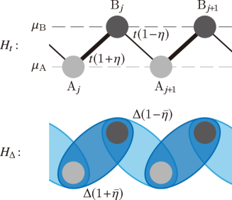
Figure 1: Schematic illustration of the SC SSH model. Top: SSH model with chemical potential imbalance between sublattices A and B. Bottom: representation of the considered pair potential, which includes pairing of states of the same cell (A-B inter-sublattice pairing) and pairing of states in neighboring cells (A-B inter-sublattice pairing).

We also explore possible measurable signatures of the obtained bulk odd-$\omega$ correlations in the SC SSH model. We find that the DOS develops higher energy pseudo-gaps, whose existence correlates with the emergence of odd-$\omega$ amplitudes, similar to what has been reported for certain multiband superconductors.Black-Schaffer and Balatsky (2013b) Furthermore, we discover that the inter-sublattice odd-$\omega$ amplitudes are finite when each sublattice has a different chemical potential, an effect that also gives rise to a finite charge density wave (CDW),Deutschmann et al. (2001); Gangadharaiah et al. (2012); Ezawa et al. (2013); Szumniak et al. (2019) whose non-zero value then automatically signals the emergence of inter-sublattice odd-$\omega$ correlations. Lastly, we find that the emergence of MZMs, e.g. as a zero energy peak in local density of states (LDOS), is a clear signal of large inter- and intra-sublattice odd-$\omega$ amplitudes. Odd-$\omega$ correlations can thus provide fundamental understanding of specific features in the DOS and CDW state in the SC SSH model.

The remainder of this article is organized as follows. In Sec. II we present the model and outline the employed method. In Sec. III we present our results demonstrating the emergence of bulk odd-$\omega$ pairing. We then, in the same section, study the relation to superconducting fitnessRamires et al. (2018); Ramires and Sigrist (2019) and show that it captures the conditions for odd-$\omega$ pairing. In Sec. IV, we discuss odd-$\omega$ pairing in the finite length SC SSH model. In Sec. V, we explore some of the possible signatures of bulk odd-$\omega$ correlations. Finally, we present our conclusions in Sec. VI.

II Model and method

We consider the SC SSH model with intra- and inter-sublattice superconducting pairing as schematically shown in Fig. 1 and modeled in real space by $H=H_{\rm t}+H_{\Delta}$, with

$$\begin{split}H_{\rm t}&=-\sum_{j}\Big{[}\mu_{\rm A}c^{\dagger}_{{\rm A},j}c_{{\rm A},j}+\mu_{\rm B}c^{\dagger}_{{\rm B},j}c_{{\rm B},j}\Big{]}\\ &-t\sum_{j}\Big{[}(1+\eta)c^{\dagger}_{{\rm B},j}c_{{\rm A},j}+(1-\eta)c^{\dagger}_{{\rm A},j+1}c_{{\rm B},j}+{\rm H.c.}\Big{]}\,,\\ H_{\Delta}&=\Delta\sum_{j}\Big{[}(1+\bar{\eta})c^{\dagger}_{{\rm B},j}c^{\dagger}_{{\rm A},j}+(1-\bar{\eta})c^{\dagger}_{{\rm A},j+1}c^{\dagger}_{{\rm B},j}+{\rm H.c.}\Big{]}\,,\end{split}$$ (1)

where $c_{\mathrm{A(B)},j}$ $(c_{\mathrm{A(B)},j}^{\dagger})$ is an annihilation (creation) operator on $j$-th cell and A(B) sublattice. Note that Eq. (1) is in real space and models the finite length SC SSH system. The first and second lines in Eq. (1) correspond to the usual SSH model in the normal state but where each sublattice A and B have a different chemical potential $\mu_{\mathrm{A,B}}$, thus giving rise to a CDW.Ezawa et al. (2013) The hopping between sites/sublattices is represented by $t>0$, with $\eta$ being the staggering parameter in the hopping term. The third term is the superconducting pairing,Wakatsuki et al. (2014); Sticlet et al. (2014) where pairing occurs between A and B sublattices both in the same cell $j$ and also between neighboring cells, with $\Delta$ being the pair potential and $\bar{\eta}$ models the staggering in the pair potential. This represents the simplest possible pairing in the SC SSH model and has been shown to be relevant in previous studies.Wakatsuki et al. (2014); Sticlet et al. (2014) Here the staggering in the hopping and pairing, caused by non-zero $\eta$ and $\bar{\eta}$, assumed real without loss of generality, is an intrinsic property of the SC SSH model. Moreover, the imbalance of chemical potentials between the A and B sublattices in Eq. (1) gives rise to a CDW gapEzawa et al. (2013) of $\mu_{\rm A}-\mu_{\rm B}$ in the normal energy versus momentum dispersion (see below) which will be relevant when looking at signatures of odd-$\omega$ pairing in experimental observables.

In order to visualize the emergence of bulk odd-$\omega$ pair correlations, we perform the analysis in momentum space, as is common for bulk properties. We first Fourier transform Eq. (1) into momentum space, which in the Nambu basis $\Psi_{k}=(c_{{\rm A},k},c_{{\rm B},k},c^{\dagger}_{{\rm A},-k},c^{\dagger}_{{\rm B},-k})$, then reads,

$$H(k)=\begin{pmatrix}H_{0}(k)&\Delta(k)\\ \Delta^{\dagger}(k)&-H_{0}^{*}(-k)\end{pmatrix}$$ (2)

where

$$H_{0}(k)=\begin{pmatrix}-\mu_{\rm A}&T_{k}\\ T^{*}_{k}&-\mu_{\rm B}\end{pmatrix}\,,\quad\Delta(k)=\begin{pmatrix}0&\Delta_{k}\\ -\Delta^{*}_{k}&0\end{pmatrix}$$ (3)

and

$$\begin{split}T_{k}&=-t[(1+\eta)+(1-\eta){\rm e}^{-ika}]\,,\\ \Delta_{k}&=-\Delta[(1+\bar{\eta})-(1-\bar{\eta}){\rm e}^{-ika}]\,,\\ \end{split}$$ (4)

correspond to the staggered momentum-dependent hopping and staggered-momentum dependent pairing, respectively. From Eqs. (4), we write $\Delta_{k}=-\Delta\{[(1+\bar{\eta})-(1-\bar{\eta}){\rm cos}(ka)]+i[(1-\bar{\eta}){\rm sin}(ka)]\}$, where the first (second) term in square brackets is even (odd) in momentum $k$, and can be seen as $s$- and $p$-wave components, respectively.

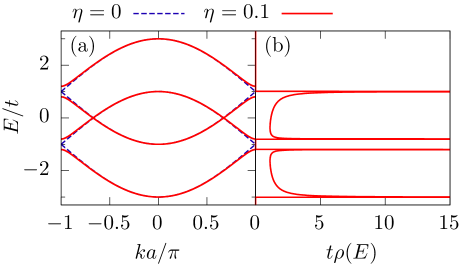
Figure 2: (a) Energy versus momentum dispersion $\pm E_{\pm}$ for $\Delta=0$, $\bar{\eta}=0$ and $\mu_{\mathrm{A}}=\mu_{\mathrm{B}}=t$ for $\eta=0$ (blue) and $\eta=0.1$ (red). (b) DOS projected on the particle space for $\eta=0.1$.

II.1 Energy versus momentum dispersion

Before going further we inspect the energy versus momentum dispersion of the SC SSH model in order to obtain an understanding of its intrinsic properties, which we later use when exploring detection schemes of odd-$\omega$ correlations. By diagonalizing Eq. (2) we obtain four energy bands given by $\pm E_{\pm}$, with

$$E_{\pm}(k)= \frac{1}{\sqrt{2}}\sqrt{\mu_{\mathrm{A}}^{2}+\mu_{\mathrm{B}}^{2}+2|T_{k}|^{2}+2|\Delta_{k}|^{2}\pm\sqrt{Y_{k}}}\,,$$ (5)

where

$$Y_{k} =4\left[{|T_{k}\Delta^{*}_{k}+T^{*}_{k}\Delta_{k}|}^{2}+|\Delta_{k}|^{2}{\left(\mu_{\mathrm{A}}-\mu_{\mathrm{B}}\right)}^{2}\right]$$

$$+4|T_{k}|^{2}{\left(\mu_{\mathrm{A}}+\mu_{\mathrm{B}}\right)}^{2}+{\left(\mu_{\mathrm{A}}^{2}-\mu_{\mathrm{B}}^{2}\right)}^{2}\,.$$ (6)

In the normal state, i.e. $\Delta=0$, the energy bands are depicted in Fig. 2(a). The electron (hole) energy bands $E_{\pm}$ ($-E_{\pm}$) cross at higher energies, $E_{+}=E_{-}$, at $k=\pm\pi/a$ when $\eta=0$, $T_{k}=0$, and $\mu_{\rm A}=\mu_{\rm B}$, as seen in blue curves in Fig. 2(a). Interestingly, when either $T_{k}\neq 0$ or $\mu_{\rm A}\neq\mu_{\rm B}$, the normal electron (hole) bands hybridize and open higher energy gaps of size $E_{+}-E_{-}$, at $k=\pm\pi/a$, see red curves in Fig. 2(a). In what follows we refer to these higher energy gaps as hybridization gaps. In particular, if $T_{k}=0$, the hybridization gap is given by $E_{+}-E_{-}=(\mu_{\rm B}-\mu_{\rm A})$, which corresponds to the CDW gapEzawa et al. (2013) due to the chemical potential imbalance between sublattices. On the other hand, when $\mu_{\rm A}=\mu_{\rm B}$, the hybridization gap is given by $E_{+}-E_{-}=2|T_{k}|$ for $\mu_{\rm A}>|T_{k}|$ or $E_{+}-E_{-}=2|\mu_{\rm A}|$ for $\mu_{\rm A}<|T_{k}|$. Remarkably, the hybridization gaps seen in the energy bands (red curves in (a)) manifest in the electronic DOS as higher energy gaps as well, as seen in Fig. 2(b).

A finite value of the pair potential, $\Delta\neq 0$, opens a gap at the Fermi points (zero-energy crossings between electron and hole bands) in the normal spectrum, as shown in Fig. 3(a-c) for different values of the chemical potentials. Interestingly, the higher energy hybridization gaps observed in the normal DOS are also partly captured in the DOS at finite $\Delta$, as seen in Fig. 4 for different values of the chemical potentials. However, since the higher energy gaps in the DOS at finite $\Delta$ are not fully developed, we refer to them as pseudo-gaps. Further details of the energy bands and DOS at finite $\Delta$ are discussed in Subsection II.2.

II.2 Winding number

The SC SSH model also exhibits interesting topological superconducting properties due to its intrinsic features. In what follows we analyze the topological phases of the SC SSH model given by Eq. (2) for a non-zero pair potential $\Delta$. In order to characterize the different topological phases in the SC SSH model we calculate the winding number associated with $H(k)$ in Eq. (2). $H(k)$ has chiral symmetry and anticommutes with a chiral operator $\Gamma=\sigma_{0}\tau_{1}$, with the winding number Sato et al. (2011) defined as

$$W=\frac{i}{4\pi}\int_{-\pi/a}^{\pi/a}\mathrm{d}k\>\mathrm{tr}\left[\Gamma H^{-1}(k)\partial_{k}H(k)\right]\,,$$ (7)

where $\sigma_{0}$ and $\tau_{1}$ are Pauli matrices in sublattice and particle-hole spaces, respectively.

In Fig. 3(d) we present the winding number $W$ as a function of $\eta$ and $\mu_{\mathrm{A}}$ for $\Delta/t=0.1$, $\mu_{\rm B}/t=1$, $\bar{\eta}=0.2$. As can be seen, depending on the system parameters, $W$ takes the values $0$ and $\pm 1$, which corresponds to the trivial and topological phases, respectively. For instance, the topological phase with $W=1$ occurs for $\mu_{c_{1}}<\mu_{\rm A}<\mu_{c_{2}}$ for a given $\eta$, where $\mu_{c_{1,2}}$ correspond to critical values that determine the phase boundary or topological phase transition (TPT). For a finite length SC SSH model in the topological phases with $W=\pm 1$, the system hosts MZMs at its end points,Wakatsuki et al. (2014); Sticlet et al. (2014) as expected from the bulk-boundary correspondence.

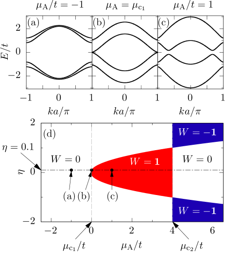
Figure 3: Energy versus momentum dispersion for (a) trivial ($\mu_{\mathrm{A}}/t=-1$), (b) topological phase transition ($\mu_{\mathrm{A}}=\mu_{\mathrm{c_{1}}}$), and (c) topological regimes ($\mu_{\mathrm{A}}/t=1$). (d) The winding number $W$ as a function of $\mu_{\mathrm{A}}$ and $\eta$, with red and blue regions corresponding to topological phases $W=\pm 1$, respectively. Parameters: $\Delta/t=0.1$, $\mu_{\mathrm{B}}/t=1$ and $\bar{\eta}=0.2$. In (a-c) $\eta=0.1$ is depicted as filled circles in (d).

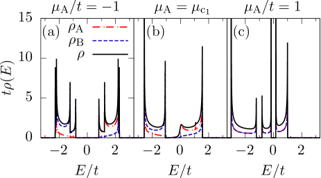
Figure 4: Particle DOS in the bulk of the SC SSH model as a function of $E$ for (a) trivial ($\mu_{\mathrm{A}}/t=-1$), (b) topological phase transition ($\mu_{\mathrm{A}}=\mu_{\mathrm{c_{1}}}$), and (c) topological ($\mu_{\mathrm{A}}/t=1$) regimes. Parameters: $\Delta/t=0.1$, $\mu_{\mathrm{B}}/t=1$, $\eta=0.1$ and $\bar{\eta}=0.2$.

Further insights to the different phases of the SC SSH model are obtained from the fact that topological phases can be distinguished by looking at the regimes where the band gap closes. To see this, in Fig. 3 (a-c) we show the energy dispersion at non-zero $\Delta$, given by Eq. (5), where we fix the parameters as in (d) and take $\eta=0.1$ but vary $\mu_{\rm A}$ such that it captures the different phases shown in (d) at the filled black circles. In the trivial phase (a), the energy gap at the Fermi energy ($E=0$) is larger than $\Delta$ since it opens even for the normal state with $\Delta=0$. At the TPT in (b), the energy gap closes and marks the topological transition point. The condition for the closing of the gap can be obtained from $E_{-}(k)=0$ leading to the following two conditions:

$$0= -\mu_{\mathrm{A}}\mu_{\mathrm{B}}+2\left[t^{2}(1+\eta^{2})-\Delta^{2}(1+\bar{\eta}^{2})\right]$$

$$+2\left[t^{2}(1-\eta^{2})+\Delta^{2}(1-\bar{\eta}^{2})\right]\cos(ka),$$ (8)

$$0= (1-\eta\bar{\eta})\sin(ka)\,.$$ (9)

which have to be simultaneously satisfied. In the topological phase (c) the energy gap is approximately given by $\Delta$ since the SC gap now opens at the Fermi points.

The pseudo-gaps in the particle DOS at finite $\Delta$, introduced in the previous subsection, in the different phases of the SC SSH model is visualized in Fig. 4. In the trivial phase, Fig. 4(a), the pseudo-gaps appear at $E/t\sim\pm 1$ due to the opening of the hybridization gap in the energy bands at $ka=\pm\pi$ in Fig. 3(a). At the topological phase transition (b), the lowest energy gap closes at the Fermi energy and there is a pseudo-gap at $E/t\sim-0.5$ due to the opening of a hybridization gap at $ka=\pm\pi$ reported in Fig. 3(b). In the topological phase (c), a small pseudo gap at $E/t\sim-1$ emerges as seen in Fig. 4(c), which is again the result of a band hybridization in the energy bands, presented in Fig. 3(c). Therefore, we conclude that band hybridization gives rise to pseudo-gaps at higher energies in the DOS of the SC SSH model, which is also similar to what occurs in certain two band superconductors.Black-Schaffer and Balatsky (2013b); Komendová et al. (2015); Asano and Sasaki (2015); Triola et al. (2020)

II.3 Green’s function method

In this work we aim at investigating the pair correlations in the SC SSH model. For this purpose we calculate the full system Green’s function,

$${\bf G}(i\omega)=\begin{pmatrix}G_{0}&F\\ \check{F}&\check{G}_{0}\end{pmatrix}={(i\omega-H)}^{-1}$$ (10)

where $H$ is given by Eq. (2) in momentum space or by Eq. (1) in real space. The matrix form of ${\bf G}$ represents the Nambu space due to the electron-hole symmetry of $H$, where $G_{0}$ and $F$ correspond to the regular and anomalous Green’s functions. Due to the basis of $H$, the structure of the Green’s function components is

$$G_{0}(i\omega)=\begin{pmatrix}G_{\rm AA}&G_{\rm AB}\\ G_{\rm BA}&G_{\rm BB}\end{pmatrix},\,F(i\omega)=\begin{pmatrix}F_{\rm AA}&F_{\rm AB}\\ F_{\rm BA}&F_{\rm BB}\end{pmatrix},$$ (11)

where $F_{\rm AA,BB}$ and $F_{\rm AB,BA}$ correspond to intra-sublattice and inter-sublattice pair correlations, originated from the sublattice indices A and B. Moreover, each element of the anomalous term $F_{ab}(i\omega)$, represents a pair amplitude with momentum $k$ or spatial coordinates in real space, frequency $\omega$, and sublattice dependence $a,b=$A, B. The sublattice index, therefore, extends the classification of Cooper pairs in this system, where the symmetries of $F_{\rm AA,BB,AB}$ determine the symmetries of the superconducting correlations and play a crucial role for the emergence of bulk odd-$\omega$ correlations in the SC SSH model, as discussed next. This view is further supported by previous studies in multiband superconductors,Black-Schaffer and Balatsky (2013b); Komendová et al. (2015); Asano and Sasaki (2015) double quantum dots,Burset et al. (2016) and double nanowiresEbisu et al. (2016b) where the band, dot, and wire indices, respectively, played the role of the sublattice index discussed here in the SC SSH model. We stress that the sublattice degree of freedom represents an intrinsic property of the SC SSH model considered in Eq. (1) and, therefore, does not depend on external considerations such as e.g., interfaces in junctions.

From the Green’s functions in Eq. (10) we can also calculate experimental observables that are important for the characterization of superconducting correlations. For instance, the normal Green’s function $G_{0}$ allows the calculation of the DOS $\rho(E)=\rho_{\mathrm{A}}(E)+\rho_{\mathrm{B}}(E)$, where

$$\begin{split}\rho_{\mathrm{A(B)}}(E)&=-\frac{1}{\pi}\mathrm{Im}\{G_{\mathrm{AA(BB)}}(i\omega=E+i\delta)\},\end{split}$$ (12)

represents the DOS at sublattice A(B), with $E$ being the real energy. We assume $\delta/\Delta=10^{-5}$ throughout this work and verify that it is sufficiently small to not alter our calculations.

III Bulk pair correlations

In this part we investigate the bulk pair correlations in the SC SSH model. By using Eq. (10) we obtain the pair amplitudes,

$$\begin{split}F_{\rm AA}(i\omega,k)&=\frac{\mu_{\rm B}(\Delta^{*}_{k}T_{k}-\Delta_{k}T^{*}_{k})-i\omega(\Delta^{*}_{k}T_{k}+\Delta_{k}T_{k}^{*})}{P(i\omega,k)}\\ F_{\rm BB}(i\omega,k)&=\frac{\mu_{\rm A}(\Delta^{*}_{k}T_{k}-\Delta_{k}T^{*}_{k})+i\omega(\Delta^{*}_{k}T_{k}+\Delta_{k}T_{k}^{*})}{P(i\omega,k)}\\ F_{\rm AB}(i\omega,k)&=\frac{1}{P(i\omega,k)}\Big{[}i\omega\Delta_{k}(\mu_{\rm B}-\mu_{\rm A})\\ &+\Delta^{*}_{k}(T_{k}^{2}-\Delta_{k}^{2})-\Delta_{k}(\omega^{2}+\mu_{\rm A}\mu_{\rm B})\Big{]}\\ F_{\rm BA}(i\omega,k)&=\frac{1}{P(i\omega,k)}\Big{[}i\omega\Delta_{k}^{*}(\mu_{\rm B}-\mu_{\rm A})\\ &-\Delta_{k}[{(T_{k}^{*})}^{2}-{(\Delta_{k}^{*})}^{2}]+\Delta_{k}^{*}(\omega^{2}+\mu_{\rm A}\mu_{\rm B})\Big{]}\,,\end{split}$$ (13)

where $P(i\omega,k)$ is a frequency and momentum dependent real polynomial in even powers of $\omega$ and $k$ whose explicit expression is not important for our discussion here but is for completeness given in Appendix A.

The main observation from Eqs. (13) is that there is a linear frequency dependent term in both the intra- $F_{\rm AA,BB}$ (second term) and inter-sublattice $F_{\rm AB,BA}$ (first term) pair amplitudes. These linear frequency components represent the odd-$\omega$ pair correlations. The odd-$\omega$ amplitudes describe a pair of electrons at different times, which vanish at equal times, thus reflecting that odd-$\omega$ pairing is an intrinsically dynamical phenomenonBergeret et al. (2005); Tanaka et al. (2012); Linder and Balatsky (2019); Cayao et al. (2019) that differs from the standard even-$\omega$ pairing. Further understanding of the pair correlations in the SC SSH model is given by analyzing the symmetries of the pair amplitudes in Eqs. (13) in terms of its frequency, momentum, and sublattice indices.

In the case of intra-sublattice amplitudes, given by the first two relations in Eqs. (13), we notice that $F_{\rm AA,BB}$ have two clear components, with the first term being even in $\omega$ and the second term being odd in $\omega$. The even-$\omega$ term, $(\Delta^{*}_{k}T_{k}-\Delta_{k}T^{*}_{k})=4it\Delta(1-\eta\bar{\eta})\sin(ka)$, is clearly odd in momentum $k$ where we have used the expressions for $\Delta_{k}$ and $T_{k}$ given by Eqs. (4). On the other hand, the odd-$\omega$ term, $\Delta^{*}_{k}T_{k}+\Delta_{k}T_{k}^{*}=4t\Delta[\eta+\bar{\eta}+(\bar{\eta}-\eta)\cos(ka)]$, is even in momentum $k$. Note that the intra-sublattice odd-$\omega$ amplitudes $F_{\rm AA,BB}$ are finite when either $\bar{\eta}$ or $\eta$ is non-zero ($t$ and $\Delta$ are always assumed to be non-zero), and thus a consequence of the intrinsic sublattice symmetry breaking in the SC SSH modelWakatsuki et al. (2014); Sticlet et al. (2014) but also predicted to appear in other systems such as in buckled quantum spin Hall insulators,Kuzmanovski and Black-Schaffer (2017) or in nanowires with Rashba spin-orbit coupling.Kobiałka et al. (2019) For $\eta=\bar{\eta}=0$ the intra-sublattice odd-$\omega$ amplitudes vanish. At $\eta\bar{\eta}=1$, however, the even-$\omega$ component is zero, leaving only finite intra-sublattice odd-$\omega$ correlations. Furthermore, the intra-sublattice pairing is automatically even (E) under the exchange of sublattice indices. This, together with the discussion above, implies that the intra-sublattice pair amplitudes given in Eqs. (13) can be classified as EEO and OEE symmetry classes in the frequency-sublattice-momentum nomenclature.

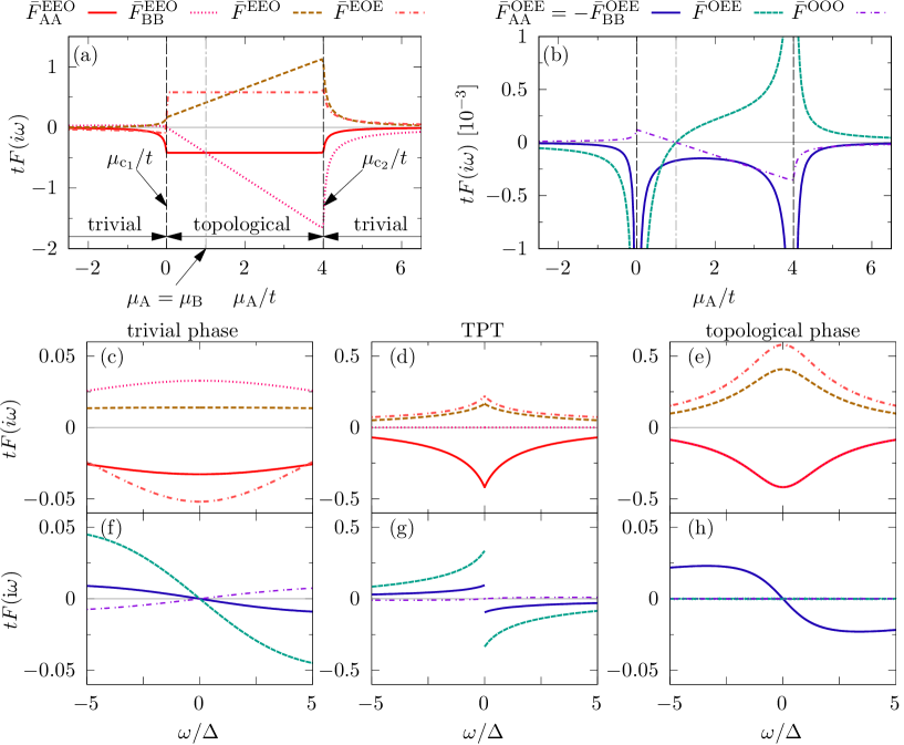
Figure 5: Bulk pair amplitudes as a function of $\mu_{\mathrm{A}}$ at $\omega/\Delta=10^{-2}$ (a,b) and $\omega$ (c-h) for $\Delta/t=0.1$, $\mu_{\mathrm{B}}/t=1$, $\eta=0.1$, and $\bar{\eta}=0.2$. Vertical dashed lines in (a,b) indicate the TPTs $\mu_{\rm c_{1,2}}$, where $\mu_{\mathrm{c_{1}}}<\mu_{\mathrm{A}}<\mu_{\mathrm{c_{2}}}$ is the topological phase. Dot-dashed vertical lines in (b) mark the points where inter-sublattice OEE and OOO vanish. Panels (c-e) and (f-h) represent the frequency dependent even- and odd-$\omega$ pair amplitudes, respectively, with $\mu_{\rm A}$ as in Fig. 3, namely, $\mu_{\mathrm{A}}/t=-1$, $\mu_{\mathrm{A}}=\mu_{\rm c_{1}}$, and $\mu_{\mathrm{A}}=t$ for the trivial, topological phase transition, and topological regimes, respectively.

For the inter-sublattice pair symmetries we proceed as in the previous paragraph, but before continuing we write the even and odd combinations under the exchange of A,B: $F_{\pm}(i\omega,k)=[F_{\rm AB}(i\omega,k)\pm F_{\rm BA}(i\omega,k)]/2$. Then, by a close inspection, we obtain that each, $F_{+}$ and $F_{-}$, has even- and odd-$\omega$ components whose symmetries are classified as OOO and OEE in the frequency-sublattice-momentum nomenclature. Their explicit expressions are: $F_{+}^{\rm OEE}(i\omega,k)=-2i\omega(\mu_{\mathrm{B}}-\mu_{\mathrm{A}})\Delta[1+\bar{\eta}+(\bar{\eta}-1)\cos(ka)]/P(i\omega,k)$ and $F_{-}^{\rm OOO}(i\omega,k)=2\omega(\mu_{\mathrm{B}}-\mu_{\mathrm{A}})\Delta(\bar{\eta}-1)\sin(ka)/P(i\omega,k)$, with an evident even and odd momentum dependence, respectively, in order to fulfill Fermi-Dirac statistics. To obtain the expressions for OOO and OEE amplitudes we have used the expression for $\Delta_{k}$ given in Eq. (4). Importantly, the non-zero value of inter-sublattice odd-$\omega$ terms, $F_{+}^{\rm OEE}$ and $F_{-}^{\rm OOO}$, is conditioned to the finite chemical potential imbalance between sublattices A and B, whose size corresponds to the CDW gap.Ezawa et al. (2013) In addition, also non-zero values of $\bar{\eta}$, $\Delta$ are needed.

Following a similar inspection as discussed above, we find that the inter-sublattice pair amplitudes $F_{\pm}$ also have even-$\omega$ components, corresponding to $F_{+}^{\rm EEO}$ and $F_{-}^{\rm EOE}$, and noticeable from the second and third terms in the last two expressions of Eqs. (13). These even-$\omega$ amplitudes represents a more standard type of superconducting pairing,Bergeret et al. (2005); Tanaka et al. (2012); Linder and Balatsky (2019); Cayao et al. (2019) which can account for pairing of electrons at equal times, unlike the odd-$\omega$ correlations.

In order to visualize the discussion made in the previous few paragraphs, we define the “$s$-wave”, which is even in $k$, and the “$p$-wave”, which is odd in $k$, components of the anomalous Green’s function, as

$$\begin{split}\bar{F}_{ab}^{s}(i\omega)&=\frac{a}{2\pi}\int_{-\pi/a}^{\pi/a}\mathrm{d}kF_{ab}(i\omega,k),\\ \bar{F}_{ab}^{p}(i\omega)&=\frac{a}{2\pi}\int_{-\pi/a}^{\pi/a}\mathrm{d}kF_{ab}(i\omega,k)\sin(ka).\end{split}$$ (14)

where $a$ and $b$ denote sublattices A or B and $F_{ab}$ correspond to the pair amplitudes given by Eqs. (13). Then, in order to account for the symmetries discussed above, we also define

$$\begin{split}\bar{F}_{\mathrm{AA(BB)}}^{\mathrm{OEE}}(i\omega)=&\mathrm{Im}\bar{F}_{\mathrm{AA(BB)}}^{s}(i\omega),\\ \bar{F}^{\mathrm{OEE}}(i\omega)=&\mathrm{Im}\bar{F}_{\mathrm{AB+BA}}^{s}(i\omega),\\ \bar{F}^{\mathrm{EOE}}(i\omega)=&\mathrm{Re}\bar{F}_{\mathrm{AB-BA}}^{s}(i\omega),\\ \bar{F}_{\mathrm{AA(BB)}}^{\mathrm{EEO}}(i\omega)=&\mathrm{Im}\bar{F}_{\mathrm{AA(BB)}}^{p}(i\omega),\\ \bar{F}^{\mathrm{EEO}}(i\omega)=&\mathrm{Im}\bar{F}_{\mathrm{AB+BA}}^{p}(i\omega),\\ \bar{F}^{\mathrm{OOO}}(i\omega)=&\mathrm{Re}\bar{F}_{\mathrm{AB-BA}}^{p}(i\omega),\end{split}$$ (15)

with $\bar{F}_{\mathrm{AB}\pm\mathrm{BA}}^{s(p)}(i\omega)=[\bar{F}_{\mathrm{AB}}^{s(p)}(i\omega)\pm\bar{F}_{\mathrm{BA}}^{s(p)}(i\omega)]/2$. In writing Eqs. (15) we have utilized that $\bar{F}_{\mathrm{AA,BB,AB+BA}}^{s(p)}$ and $\bar{F}_{\mathrm{AB-BA}}^{s(p)}$ solely exhibit imaginary and real values, respectively, as shown in Appendix B. Note also that, by using Eqs. (13), we can show that $\bar{F}_{\mathrm{AA}}^{\mathrm{OEE}}(i\omega)=-\bar{F}_{\mathrm{BB}}^{\mathrm{OEE}}(i\omega)$, and, therefore, it is only necessary to investigate and plot one of them.

In Figs. 5 we plot the pair amplitudes given by Eqs. (15) as a function of the chemical potential $\mu_{\mathrm{A}}$ at $\omega/\Delta=10^{-2}$ (a,b) and frequency $\omega$ (c-h), where in the former we also detect the different topological phases. The even-$\omega$ components develop generally larger values in the topological phase than in the trivial phase, as seen in (a). These even-$\omega$ correlations usually exhibit also larger amplitudes than the odd-$\omega$ terms in both the trivial and topological phases, as seen by comparing (a) and (b). However, at the TPTs ($\mu_{\mathrm{c_{1}}}$ and $\mu_{\mathrm{c_{2}}}$ marked with dashed vertical lines) both the intra- and inter-sublattice amplitudes $\bar{F}_{\mathrm{AA(BB)}}^{\mathrm{OEE}}$ and $\bar{F}^{\mathrm{OEE}}$ have divergent profiles with comparable or even larger values than their even-$\omega$ counterparts. The inter-sublattice OOO component also exhibits its maximum value at TPTs but with an overall smaller amplitude than the even-$\omega$ terms. The divergent values at the TPTs occur because the denominator of the pair amplitudes, $P(i\omega,k)$ in Eq. (13), has a singularity at the energy gap closing. Furthermore, at $\mu_{\mathrm{A}}=\mu_{\mathrm{B}}$ (vertical dot-dashed grey line in Fig. 5(a,b)), the inter-sublattice amplitudes $\bar{F}^{\mathrm{OEE}}$ and $\bar{F}^{\mathrm{OOO}}$ vanish, leaving only non-zero intra-sublattice odd-$\omega$ correlations with OEE symmetry. This can be also directly seen in Eqs. (13).

Next we investigate the frequency dependence of the pair amplitudes in Figs. 5(c–h). As expected, $\bar{F}_{\mathrm{AA(BB)}}^{\mathrm{EEO}}$, $\bar{F}^{\mathrm{EEO}}$, and $\bar{F}^{\mathrm{EOE}}$ exhibit an even frequency dependence with their maximum absolute value occurring at $\omega=0$ in the trivial, TPT, and topological phases, as seen in (c-e) . Likewise, the odd-$\omega$ components, $\bar{F}_{\mathrm{AA(BB)}}^{\mathrm{OEE}}$, $\bar{F}^{\mathrm{OEE}}$, and $\bar{F}^{\mathrm{OOO}}$, display the expected odd frequency dependence. However, unlike all the even-$\omega$ terms, the intra-sublattice OEE and inter-sublattice OEE amplitudes develop a discontinuous profile with a maximum magnitude around $\omega=0$ only at the TPT, which can be understood as a result of the energy gap closing at the TPT; the inter-sublattice OOO component at the TPT is instead very small and with smooth profile across $\omega=0$. In the trivial (f) and topological phases (h) all odd-$\omega$ components have a smooth and approximate linear frequency dependence at low frequencies.

We thus find that intra- and inter-sublattice odd-$\omega$ amplitudes, given by Eqs. (13), do not vanish when $T_{k}\neq 0$ and $\mu_{\rm A}\neq\mu_{\rm B}$, respectively, provided $\Delta_{k}\neq 0$. Interestingly, the presence of these bulk odd-$\omega$ correlations can be correlated with experimental observables as well. In fact, in Subsection II.2 we show that either $T_{k}\neq 0$ or $\mu_{\rm A}\neq\mu_{\rm B}$ induce a hybridization of the normal electron (hole) bands in the SC SSH model which then give rise to pseudo gaps in the DOS, as seen in Fig. 4. Therefore, this allows us to conclude that the pseudo gaps in the DOS indicates the presence of either intra- or inter-sublattice odd-$\omega$ correlations, as the conditions for these two effects to emerge coincide. We point out that these features are similar to what occurs in certain two band superconductors.Black-Schaffer and Balatsky (2013b); Komendová et al. (2015); Asano and Sasaki (2015); Triola et al. (2020)

To summarize this part, we stress that the SC SSH model hosts bulk dynamic odd-$\omega$ correlations, due to its intrinsic properties, namely, staggered hopping, staggered pair potential, and chemical potential imbalance. While even-$\omega$ correlations develop larger values than the odd-$\omega$ amplitudes in the trivial and topological phases, at the TPTs the odd-$\omega$ amplitudes exhibit a discontinuous profile with maximum magnitude whose values are comparable or even larger than even-$\omega$ amplitudes. Our findings, therefore, suggest that both even- and odd-$\omega$ correlations must be considered when studying superconductivity in the SC SSH model.

III.1 Superconducting fitness

All the conditions that we have identified so far for the emergence of finite odd-$\omega$ correlations can be elegantly obtained by calculating the superconducting fitness,Ramires et al. (2018); Ramires and Sigrist (2019) $C=H_{0}(k)\Delta(k)-\Delta(k)H^{*}_{0}(-k)$. It was demonstrated in Ref. Triola et al., 2020 that it is possible to determine the presence of odd-$\omega$ pairing in multiband superconductors when $C\neq 0$. By plugging Eqs. (3) into $C$, we obtain the following conditions

$$\begin{split}(\mu_{\rm A}-\mu_{\rm B})\Delta_{k}&\neq 0,\\ T_{k}\Delta^{*}_{k}+\Delta_{k}T^{*}_{k}&\neq 0\,,\end{split}$$ (16)

where only one of these expressions needs to be satisfied in order for odd-$\omega$ pairing to appear.

The finite value of the odd-$\omega$ amplitudes, obtained from Eqs. (13), is fully consistent with the expressions derived from the superconducting fitness in Eqs. (16). In fact, the first condition in Eqs. (16), clearly reflects the need of a chemical potential imbalance, which is indeed the necessary condition for finite inter-sublattice odd-$\omega$ correlations, $F_{\rm AB,BA}$, as can be seen in Eqs. (13). Similarly, the second condition captures the non-zero intra-sublattice odd-$\omega$ correlations, $F_{\rm AA,BB}$ in Eqs. (13).

IV Pair correlations in the finite size SC SSH model

After showing that bulk odd-$\omega$ correlations emerge in the SC SSH model, we next explore the odd-$\omega$ amplitudes when the system has a finite size and is modeled in real space by Eq. (1). This is particularly motivated because it has been shown that, in the topological phase, the SC SSH model hosts MZMs,Wakatsuki et al. (2014); Sticlet et al. (2014) and MZMs have been predicted to enhance odd-$\omega$ amplitudes at the edges of topological superconductors, Tanaka et al. (2012); Asano and Tanaka (2013); Black-Schaffer and Balatsky (2013a); Ebisu et al. (2015); Ikegaya et al. (2015); Crépin et al. (2015); Huang et al. (2015); Kashuba et al. (2017); Ebisu et al. (2016b); Lee et al. (2017); Cayao and Black-Schaffer (2017); Tanaka and Tamura (2018); Keidel et al. (2018); Fleckenstein et al. (2018); Tsintzis et al. (2019); Cayao et al. (2019); Kuzmanovski et al. (2019) although they have not yet been investigated in the context of the SC SSH model.

We use a tight-binding representation for the SC SSH Hamiltonian, given by Eq. (1), in Nambu space with $N$ lattice unit cells and lattice spacing $a$ in the basis $(c_{\mathrm{A},1},c_{\mathrm{A},1}^{\dagger},c_{\mathrm{B},1},c_{\mathrm{B},1}^{\dagger},\dots,c_{\mathrm{B},N},c_{\mathrm{B},N}^{\dagger})$. The position coordinate is then denoted as $x=ja$ with unit cell index $j$, being $1\leq j\leq N$, and system size $L=100a$. We then obtain the pair amplitudes from the anomalous component of the Green’s function $g_{j_{1},j_{2}}(i\omega)={(i\omega-H)}_{j_{1},j_{2}}^{-1}$, where $j_{1,2}$ corresponds to two lattice sites in the tight-binding representation. The Green’s function $g$ has $4N\times 4N$ elements due to the sublattice and particle-hole symmetries. Similarly, as for the discussion of the bulk pair amplitudes in Sec. III, in what follows we decompose the anomalous term of $g$ into the symmetry classes defined in Eqs. (15), which can be written as

$$f_{\mathrm{AA(BB)}}^{\mathrm{OEE}}(i\omega,j)= \mathrm{Im}f_{\mathrm{AA(BB)}}^{\mathrm{intra}}(i\omega,j),$$ (17)

$$f^{\mathrm{OEE}}(i\omega,j)= \mathrm{Im}f_{\mathrm{AB+BA}}^{\mathrm{intra}}(i\omega,j),$$ (18)

$$f^{\mathrm{EOE}}(i\omega,j)= \mathrm{Re}f_{\mathrm{AB-BA}}^{\mathrm{intra}}(i\omega,j),$$ (19)

$$f_{\mathrm{AA(BB)}}^{\mathrm{EEO}}(i\omega,j)= \mathrm{Im}f_{\mathrm{AA(BB)}}^{\mathrm{n.n.}}(i\omega,j),$$ (20)

$$f^{\mathrm{EEO}}(i\omega,j)= \mathrm{Im}f_{\mathrm{AB+BA}}^{\mathrm{n.n.}}(i\omega,j),$$ (21)

$$f^{\mathrm{OOO}}(i\omega,j)= \mathrm{Re}f_{\mathrm{AB-BA}}^{\mathrm{n.n.}}(i\omega,j),$$ (22)

where

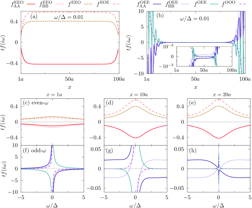
Figure 6: Pair amplitudes in the topological phase of the finite length SC SSH model with $L=100a$ as a function of (a,b) spatial coordinate $x=ja$ and (c-h) frequency. In (a,b) $\omega/\Delta=10^{-2}$. The inset in (b) magnifies the view of the odd-$\omega$ amplitudes in the bulk. In panels (c,f), (d,g), and (e,h) the frequency dependence of the pair amplitudes is plotted for $x=1a$, $x=10a$, and $x=20a$, respectively. Parameters: $\Delta/t=0.1$, $\mu_{\rm A,B}=t$, $\eta=0.1$, and $\bar{\eta}=0.2$, see Fig. 3(c).

$$\begin{split}f_{\mathrm{AA}}^{\mathrm{intra}}(i\omega,j)&=g_{4j-3,4j-2}(i\omega),\\ f_{\mathrm{BB}}^{\mathrm{intra}}(i\omega,j)&=g_{4j-1,4j}(i\omega),\\ f_{\mathrm{AB\pm BA}}^{\mathrm{intra}}(i\omega,j)&=\frac{1}{\sqrt{2}}\left[g_{4j-3,4j}(i\omega)\pm g_{4j-1,4j-2}(i\omega)\right],\\ f_{\mathrm{AA}}^{\mathrm{n.n.}}(i\omega,j)&=\frac{1}{2\mathrm{i}}\left[g_{4j-3,4j+2}(i\omega)-g_{4j+1,4j-2}(i\omega)\right],\\ f_{\mathrm{BB}}^{\mathrm{n.n.}}(i\omega,j)&=\frac{1}{2\mathrm{i}}\left[g_{4j-1,8j}(i\omega)-g_{4j+3,4j}(i\omega)\right],\\ f_{\mathrm{AB\pm BA}}^{\mathrm{n.n.}}(i\omega,j)&=\frac{1}{2\sqrt{2}\mathrm{i}}\left\{\left[g_{4j-3,8j}(i\omega)-g_{4j+1,4j}(i\omega)\right]\right.\\ &\left.\pm\left[g_{4j-1,4j+2}(i\omega)-g_{4j+3,4j-2}(i\omega)\right]\right\},\end{split}$$ (23)

correspond to intra- and nearest-neighbor (n.n) unitcell components. We have checked that Eqs. (17), (18), (20), and (21) have only imaginary parts, while Eqs. (19) and (22) only real, which is taken into account when discussing them next. These pair amplitudes allow us to make a direct comparison with the results found in the bulk system in the previous section and displayed in Fig. 5. In fact, we have verified that in the bulk, at $x=L/2$ with sufficiently large $L$, i.e. far from both edges, the amplitudes obtained from Eqs. (17)-(22) coincide with the amplitudes obtained with Eqs. (15), respectively.

To proceed we concentrate on the topological phase where MZMs emerge at both edges. In Fig. 6 we present the pair amplitudes as a function of space and frequency. Here, the superconducting coherence length is approximately $4a$, which then indicates that the system size is much larger than the coherence length. At low frequencies, all the even-$\omega$ amplitudes show roughly constant values in the bulk away from the edges for $x\gtrsim 10a$, Takagi et al. (2020) while at the edges they exhibit reduced but finite values, as seen in (a). On the other hand, the low-frequency odd-$\omega$ components develop a huge increase near the edges, from where they decay, but do not vanish, towards the bulk of the system in an exponentially oscillatory fashion (b). We attribute this enhancement to the emergence of MZMs in the topological phase, in a similar way as in other topological systems.Tanaka et al. (2012); Asano and Tanaka (2013); Black-Schaffer and Balatsky (2013a); Ebisu et al. (2015); Ikegaya et al. (2015); Crépin et al. (2015); Huang et al. (2015); Kashuba et al. (2017); Ebisu et al. (2016b); Lee et al. (2017); Cayao and Black-Schaffer (2017); Tanaka and Tamura (2018); Keidel et al. (2018); Fleckenstein et al. (2018); Tsintzis et al. (2019); Cayao et al. (2019); Kuzmanovski et al. (2019) Moreover, in order to identify the emergence of odd-$\omega$ amplitudes in the bulk as well as compare with the results presented in the previous section, we present in the inset of Fig. 6(b), a magnified view. This probes the pair amplitudes for small $\omega/\Delta=10^{-2}$ in the center of the system, at $x\sim 50a$. Notice that the values of the odd-$\omega$ components are almost the same as those shown in Fig. 5(b) with $\mu_{\mathrm{A}}/t=1$. Likewise, we have verified that the even-$\omega$ terms at $x=50a$ coincide with those obtained using Eqs. (15). Moreover, we stress that $f_{\mathrm{AA}}^{\mathrm{OEE}}=-f_{\mathrm{BB}}^{\mathrm{OEE}}$ is only satisfied far from both edges, in agreement with what we discuss after Eqs. (15).

Next we turn our discussion to the frequency dependence of the pair amplitudes, presented in Figs. 6(c-h) for different locations in space. First, all the pair amplitudes have the expected even- or odd-$\omega$ dependence but the odd-$\omega$ correlations exhibit a dramatic change of behavior depending on if they are calculated in the center of the system at $x=L/2$ or at the edge at $x=1a$. At the edge, all the odd-$\omega$ terms develop a drastic increase at low frequencies with a divergent profile, supporting the idea that their huge values originate due to the presence of a MZM.Tanaka et al. (2012); Asano and Tanaka (2013); Black-Schaffer and Balatsky (2013a); Ebisu et al. (2015); Ikegaya et al. (2015); Crépin et al. (2015); Huang et al. (2015); Kashuba et al. (2017); Ebisu et al. (2016b); Lee et al. (2017); Cayao and Black-Schaffer (2017); Tanaka and Tamura (2018); Keidel et al. (2018); Fleckenstein et al. (2018); Tsintzis et al. (2019); Cayao et al. (2019); Kuzmanovski et al. (2019) At $x=10a$ the odd-$\omega$ amplitudes acquire smaller values but still large variations in their frequency dependence. This is more clearly seen at $x=20a$ where the huge values of odd-$\omega$ amplitudes around $\omega\approx 0$, seen at the edge, is more narrow but still large. We have checked that deep in the bulk, $x=50a$ for this case, the odd-$\omega$ correlations in the finite size SC SSH model recover the behavior presented in Fig. 5(h). On the contrary, the even-$\omega$ terms at $x=1a$ exhibits a smooth behavior as a function of frequency with non-zero values and a maximum value around low frequencies, as seen in (c). Moving towards the bulk, at $x=10a,20a$, the frequency dependence of the even-$\omega$ amplitudes is preserved, but they acquire larger values, as presented in (d,e).

IV.1 Spectral bulk-boundary correspondence

Further understanding of the relation between odd-$\omega$ correlations and the topological phase can be obtained from a spectral bulk-boundary correspondence (SBBC).Tamura et al. (2019); Daido and Yanase (2019) The SBBC tells us that some components of the anomalous Green’s function are related to an extended version of the winding number defined in the bulk for chiral symmetric systems. For the SC SSH model, which is chiral symmetric, with open boundary conditions, the amount of intra-sublattice odd-$\omega$ components at the edge is given by

$$F_{L=Na}(i\omega)=2i\sum_{j=1}^{N/2}\left[f_{\mathrm{AA}}^{\mathrm{OEE}}(i\omega,j)+f_{\mathrm{BB}}^{\mathrm{OEE}}(i\omega,j)\right]\,.$$ (24)

We point out that it is due to the special form of the chiral operator for the SC SSH model, discussed in Appendix C, that only the intra-sublattice components OEE appear in the previous expression. Then, following Refs. Tamura et al., 2019; Daido and Yanase, 2019, we numerically find that, at small $\omega$, the previous expression can be written as

$$\lim_{N\rightarrow\infty}F_{L=Na}(i\omega)=W/(i\omega)+i\chi\omega+\mathcal{O}(\omega^{3})\,,$$ (25)

where $W$ is the winding number, given by Eq. (7), and $\chi$ is a real number. Details about the derivation can also be found in Appendix C.

By a simple inspection of Eq. (25), we notice that $F_{L=Na}(i\omega)$ diverges at low frequencies in the topological phase ($W=\pm 1$), while it is a linear function of $\omega$ in the trivial phase ($W=0$). This frequency dependence is in agreement with the divergent behavior in the topological phase of the low-frequency intra-sublattice pair correlations at the edge in Fig. 6(f). Interestingly, Eq. (25) indicates that it is possible to calculate some of the odd-$\omega$ correlations at the edge of the SC SSH model, which is an edge property, simply by calculating the winding number $W$ by Eq. (7), which is a bulk property of the system. Moreover, even though both topological phases ($W=\pm 1$) host MZMs at the system ends, their associated odd-frequency pair amplitudes exhibit opposite sign, as seen in Eq. (25).

V Further experimental consequences

As we mentioned in Sec.  II, the imbalance between the chemical potentials in sublattices A and B allow for a CDW.Ezawa et al. (2013) In order to characterize the CDW, which is due to a chemical potential imbalance, we define the CDW Green’s function as the imbalance between regular Green’s functions at sublattices A and B, namely, $G_{\rm CDW}=G_{\mathrm{AA}}-G_{\mathrm{BB}}$, where $G_{\mathrm{AA,BB}}$ are obtained from Eqs. (10) and (11). Then, we obtain

$$\begin{split}G_{\rm CDW}(i\omega,k)&=\left(\mu_{\mathrm{A}}-\mu_{\mathrm{B}}\right)[{-(i\omega)}^{2}+\left(\mu_{\mathrm{A}}+\mu_{\mathrm{B}}\right)i\omega\\ &+\left(|T_{k}|^{2}-|\Delta_{k}|^{2}-\mu_{\mathrm{A}}\mu_{\mathrm{B}}\right)]/P(i\omega,k),\end{split}$$ (26)

where $P(i\omega,k)$ is the same real polynomial as in Eqs. (13) with even powers of $\omega$ and $k$. Interestingly, Eq. (26) is non-zero if $\mu_{\mathrm{A}}\neq\mu_{\mathrm{B}}$, the condition that also allows for finite inter-sublattice odd-$\omega$ amplitudes, as seen in Eqs. (13) and  (16). Thus, a finite CDW is a good indicator of non-zero inter-sublattice odd-$\omega$ amplitudes. For a further interpretation and understanding, we define

$$\begin{split}G_{\rm CDW}^{\mathrm{E}}(i\omega)&=\mathrm{Re}G_{\rm CDW}(i\omega),\\ G_{\rm CDW}^{\mathrm{O}}(i\omega)&=\mathrm{Im}G_{\rm CDW}(i\omega),\\ G_{\rm CDW}(i\omega)&=\frac{a}{2\pi}\int_{-\pi/a}^{\pi/a}\mathrm{d}k\>G_{\mathrm{CDW}}(i\omega,k)\,,\end{split}$$ (27)

where $G_{\rm CDW}^{\mathrm{E(O)}}$ are even and odd functions of $\omega$, respectively. The behavior of these two quantities is shown in Fig. 7(a-c). In panel (a) $G_{\mathrm{CDW}}^{\mathrm{E(O)}}$ is presented at low frequencies ($\omega/\Delta=10^{-2}$) as a function of $\mu_{\mathrm{A}}$. The main feature here is that both $G_{\mathrm{CDW}}^{\mathrm{E,O}}$ take large values at the TPTs at $\mu_{\mathrm{A}}=\mu_{\mathrm{c_{1}}}$ and $\mu_{\mathrm{A}}=\mu_{\mathrm{c_{2}}}$. As we move away from the TPTs, $G_{\mathrm{CDW}}^{\mathrm{O}}$ acquires very small values since it is an odd function of $\omega$ and we are here also at small $\omega$. On the other hand, $G_{\mathrm{CDW}}^{\mathrm{E}}$ in the trivial phase develops smaller, but finite, values than in the topological phase. The frequency dependence of $G_{\mathrm{CDW}}^{\mathrm{E,O}}$ is shown in panels (b,c) for $\mu_{\mathrm{A}}/t=-1$, $0$ and $1$, values that correspond to the trivial phase, TPT, and topological phase, respectively, also used in Fig. 3(a-c). These two panels allow us to conclude that $G_{\mathrm{CDW}}^{\mathrm{E,O}}$ indeed represent even and odd-$\omega$ CDWs, respectively, where the latter was also predicted to appear in other systems.Pivovarov and Nayak (2001); Kedem and Balatsky (2015)

Although the condition $\mu_{\mathrm{A}}\neq\mu_{\mathrm{B}}$ simultaneously allows for finite CDW and inter-sublattice odd-$\omega$ correlations, $F_{+}^{\mathrm{OEE}}$, it is important to disentangle which of the CDWs captures the behavior of $F_{+}^{\mathrm{OEE}}$. The dependence on $\mu_{\rm A}$ can be observed in the inset of Fig. 7(a) and it has to be compared with Fig. 5(b), where we see that both quantities exhibit large values at the TPTs and sign change at $\mu_{\mathrm{A}}=\mu_{\mathrm{B}}$. Moreover, the frequency dependence of the odd-$\omega$ CDW and $F_{+}^{\mathrm{OEE}}$ at the TPT is also similar, with a maximum and sharp sign change at $\omega=0$, as seen by comparing Figs. 7(c) and Fig. 5(g). We, therefore, conclude that $F_{+}^{\mathrm{OEE}}$ and the odd-$\omega$ CDW exhibit a similar qualitative behavior. We can, therefore, conclude that the emergence of a CDW signals the presence of inter-sublattice odd-$\omega$ correlations, as both occur due to a chemical potential imbalance between sublattices in the SC SSH model. This chemical potential imbalance is due to modulations of the chemical potentials,Gangadharaiah et al. (2012) obtained e.g. via electrically tunable gates.Deutschmann et al. (2001); Szumniak et al. (2019) We argue that the CDW can be measured as an imbalance of DOSs between sublattices, thus allowing a way to obtain the inter-sublattice odd-$\omega$ correlations.

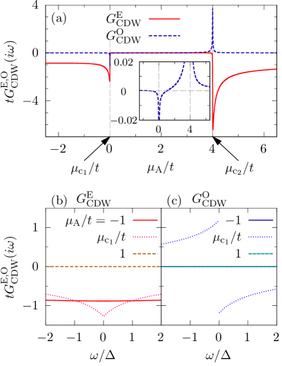
Figure 7: (a) $G_{\mathrm{CDW}}^{\mathrm{E}}(i\omega)$ and $G_{\mathrm{CDW}}^{\mathrm{O}}(i\omega)$ as a function of $\mu_{\mathrm{A}}$ at $\omega/\Delta=10^{-2}$ for $\Delta/t=0.1$, $\mu_{\mathrm{B}}/t=1$, $\eta=0.1$, and $\bar{\eta}=0.2$. Inset of (a) shows a magnified view of $G_{\mathrm{CDW}}^{\mathrm{O}}(i\omega)$. (b,c) Frequency dependence of $G_{\mathrm{CDW}}^{\mathrm{E,O}}(I\omega)$ for $\mu_{\mathrm{A}}/t=-1$, $\mu_{\mathrm{c}_{1}}/t$, and $1$ with $\Delta/t=0.1$, $\mu_{\mathrm{B}}/t=1$, $\eta=0.1$, and $\bar{\eta}=0.2$.

VI Conclusions

We investigated the superconducting pair symmetries in the superconducting Su-Schrieffer-Heeger model and demonstrated that this system hosts bulk odd-frequency pair correlations in the trivial and topological phases, due to its intrinsic staggered properties. In particular, we found that the sublattice degree of freedom is responsible for extending the classification of pair correlations, thus allowing a coexistence of inter- and intra-sublattice even- and odd-frequency amplitudes. The odd-frequency correlations depend on the staggered hopping and chemical potential imbalance between sublattices, provided there is a non-zero pair potential, conditions that are also consistent with the non-zero value of the superconducting fitness.

In the topological phase in finite length systems we showed that the low-frequency odd-frequency amplitudes are enhanced at the edges of the system due to the presence of Majorana zero modes. Furthermore, we demonstrated that the spectral bulk boundary correspondence reveals the relation between intra-sublattice odd-frequency correlations and winding number, thus extending previous studiesTamura et al. (2019); Daido and Yanase (2019) to systems with intrinsic staggering, such as the SC SSH model. Our results highlight odd-frequency pairing as a bulk phenomenon that goes beyond the induced effect in junctions and does not require any external actor, such as interfaces in junctions, but instead, this bulk effect solely relies on the intrinsic staggered nature of the system.

Lastly, we analyzed some of the possible experimental signals that can be correlated with odd-frequency amplitudes. First, we showed that a finite staggered hopping or chemical potential imbalance gives rise to pseudo gaps in the DOS, which then signal the presence of intra- or inter-sublattice odd-frequency amplitudes, respectively. Second, we found that the finite chemical potential imbalance between sublattices gives rise to a charge density wave whose odd-frequency component develops a qualitatively equivalent behavior as the inter-sublattice odd-frequency amplitude. These modulations in the chemical potential can be induced via e.g. electrically tunable gates,Gangadharaiah et al. (2012); Deutschmann et al. (2001); Szumniak et al. (2019) where the charge density wave can be measured as the imbalance of DOSs between sublattices. Finally, for a finite system length, the zero energy peak in the LDOS, which reflects the emergence of a Majorana zero mode at the edges of the system, directly indicates the presence of large inter- and intra-sublattice odd-frequency correlations.

VII Acknowledgements

We thank P. Burset and O. A. Awoga for helpful discussions. S. T., S. N., and Y. T. acknowledge the support from Grant-in-Aid for Scientific Research on Innovative Areas, Topological Material Science (Grants No. JP15H05851, No. JP15H05853, and No. JP15K21717) and Grant-in-Aid for Scientific Research B (KAKENHI Grant No. JP18H01176) from the Ministry of Education, Culture, Sports, Science, and Technology, Japan (MEXT) and JST CREST Grant No. JPMJCR16F2. Y. T. is also supported by Scientific Research A (KAKENHI Grant No. JP20H00131) and JSPS Core-to-Core program “Oxide Superspin international network”. A. B. S. and J. C. acknowledge support from the Swedish Research Council (Vetenskapsrådet Grant No. 2018-03488), the Knut and Alice Wallenberg Foundation through the Wallenberg Academy Fellows program, and the European Research Council (ERC) under the European Unions Horizon 2020 Research and Innovation Programme (ERC-2017-StG-757553).

Appendix A Denominator of the bulk Green’s function

The denominator of the bulk Green’s function in Eq. (13) is given by

$$P(i\omega,k)= {(i\omega)}^{4}-\left[2\left({|T_{k}|}^{2}+{|\Delta_{k}|}^{2}\right)+\mu_{\mathrm{A}}^{2}+\mu_{\mathrm{B}}^{2}\right]{(i\omega)}^{2}$$

$$+{|T_{k}^{2}-\Delta_{k}^{2}|}^{2}-2\left({|T_{k}|}^{2}-{|\Delta_{k}|}^{2}\right)\mu_{\mathrm{A}}\mu_{\mathrm{B}}$$

$$+{\left(\mu_{\mathrm{A}}\mu_{\mathrm{B}}\right)}^{2}\,.$$ (28)

By simple inspection, we verify that $P(i\omega,k)$ is a real number for real $\omega$ and an even function of $\omega$. Moreover, it is also even in $k$ since $T_{k}^{2}$, $\Delta_{k}^{2}$ and ${|T_{k}^{2}-\Delta_{k}|}^{2}$ are all even in $k$. This can be seen by writing the following expressions,

$${|T_{k}|}^{2}= t^{2}\left[{(1+\eta)}^{2}+{(1-\eta)}^{2}+2(1-\eta^{2})\cos(ka)\right],$$ (29)

$${|\Delta_{k}|}^{2}= \Delta^{2}\left[{(1+\bar{\eta})}^{2}+{(1-\bar{\eta})}^{2}-2(1-\bar{\eta}^{2})\cos(ka)\right],$$ (30)

$${|T_{k}^{2}-\Delta_{k}|}^{2}= {|T_{k}|}^{4}+{|\Delta_{k}|}^{4}-2\mathrm{Re}{(T_{k}\Delta_{k}^{*})}^{2}\,,$$ (31)

where we have used the definitions of $T_{k}$ and $\Delta_{k}$ given by Eqs. (4) in the main text. Then, we conclude that $P(i\omega,k)$ satisfies $P(-i\omega,-k)=P(i\omega,k)$, conditions that are used when discussing the properties of the Green’s function given by Eq. (13) in the main text.

Appendix B Real and imaginary parts of the bulk pair amplitudes

In this appendix we explain why we take the real and imaginary parts of the bulk pair amplitudes given in Eqs. (15). In Eqs. (13), the real and imaginary parts of $\Delta_{k}^{*}T_{k}$, $\Delta_{k}$ and $\Delta_{k}^{*}(T_{k}^{2}-\Delta_{k}^{2})$ are given by

$$\begin{split}\mathrm{Re}\Delta_{k}^{*}T_{k}&=2t\Delta\left[(\eta+\bar{\eta})+(-\eta+\bar{\eta})\cos(ka)\right],\\ \mathrm{Im}\Delta_{k}^{*}T_{k}&=-2i\Delta t\left[1-\eta\bar{\eta}\sin(ka)\right],\\ \mathrm{Re}\Delta_{k}&=-\Delta\left[(1+\bar{\eta})-(1-\bar{\eta})\cos(ka)\right],\\ \mathrm{Im}\Delta_{k}&=-i\Delta(1-\bar{\eta})\sin(ka),\\ \mathrm{Re}\Delta_{k}^{*}(T_{k}^{2}-\Delta_{k}^{2})&=\Delta\left[t^{2}(1+\eta)^{2}-\Delta^{2}(1+\bar{\eta})^{2}\right][-(1+\bar{\eta})+(1-\bar{\eta})\cos(ka)]\\ &+2\Delta\left[t^{2}(1-\eta^{2})+\Delta^{2}(1-\bar{\eta}^{2})\right][-(1+\bar{\eta})\cos(ka)+(1-\bar{\eta})]\\ &+2\Delta\left[t^{2}(1-\eta)^{2}-\Delta^{2}(1-\bar{\eta})^{2}\right][-(1+\bar{\eta})\cos(2ka)+(1-\bar{\eta})\cos(ka)],\\ \mathrm{Im}\Delta_{k}^{*}(T_{k}^{2}-\Delta_{k}^{2})&=i\Delta(1-\bar{\eta})\left[t^{2}(1+\eta)^{2}-\Delta^{2}(1+\bar{\eta})^{2}\right]\sin(ka)+2i\Delta(1+\bar{\eta})\left[t^{2}(1-\eta^{2})+\Delta^{2}(1-\bar{\eta}^{2})\right]\sin(ka)\\ &-i\Delta\left[t^{2}(1-\eta)^{2}-\Delta^{2}(1-\bar{\eta})^{2}\right][-(1+\bar{\eta})\sin(2ka)+(1-\bar{\eta})\sin(ka)].\end{split}$$ (32)

First, by using previous equations, $F_{\mathrm{AA(BB)}}^{s}(i\omega)$ from Eqs. (14) is given by

$$F_{\mathrm{AA}}^{s}(i\omega)= -F_{\mathrm{BB}}^{s}(i\omega)$$

$$= -i\frac{a}{2\pi}\int_{-\pi/a}^{\pi/a}\mathrm{d}k\frac{\omega(\Delta_{k}^{*}T_{k}+\Delta_{k}T_{k}^{*})}{P(i\omega,k)}\,,$$ (33)

where we can see that $F_{\mathrm{AA(BB)}}^{s}(i\omega)$ is an odd function of $\omega$, since $P(i\omega,k)$ is real, and an even function of $\omega$ and $\mathrm{Re}F_{\mathrm{AA(BB)}}^{s}(i\omega)=0$. Hence, we set $F_{\mathrm{AA(BB)}}^{\mathrm{OEE}}(i\omega)=\mathrm{Im}F_{\mathrm{AA(BB)}}^{s}(i\omega)$, which is the first equation written in Eqs. (15).

Second, similarly as before, $F^{s}_{\mathrm{AB+BA}}(i\omega)$ is given by

$$F_{\mathrm{AB+BA}}^{s}(i\omega)= \frac{i\omega a}{2\pi}\int_{-\pi/a}^{\pi/a}\mathrm{d}k\frac{(\Delta_{k}+\Delta_{k}^{*})(\mu_{\mathrm{B}}-\mu_{\mathrm{A}})}{P(i\omega,k)}.$$ (34)

By using Eqs. (32), we obtain that this quantity is purely imaginary and an odd function of $\omega$. Then, we set $F^{\mathrm{OEE}}(i\omega)=\mathrm{Im}F_{\mathrm{AB+BA}}^{s}(i\omega)$, which is the second equation in Eqs. (15).

Third, $F^{s}_{\mathrm{AB-BA}}(i\omega)$ is given by

$$F_{\mathrm{AB-BA}}^{s}(i\omega)$$

$$= \frac{a}{\pi}\int_{-\pi/a}^{\pi/a}\mathrm{d}k\frac{\mathrm{Re}[\Delta_{k}^{*}(T_{k}^{2}-\Delta_{k}^{2})-\Delta_{k}(\omega^{2}+\mu_{\mathrm{A}}\mu_{\mathrm{B}})]}{P(i\omega,k)},$$ (35)

which is purely real and an even function of $\omega$. Then, we set $F^{\mathrm{EOE}}(i\omega)=\mathrm{Re}F_{\mathrm{AB+BA}}^{s}(i\omega)$, giving rise to the third line in Eqs. (15).

Fourth, $F_{\mathrm{AA(BB)}}^{p}(i\omega)$ is

$$\begin{split}&F_{\mathrm{AA(BB)}}^{p}(i\omega)=\\ &=\frac{a}{2\pi}\int_{-\pi/a}^{\pi/a}\mathrm{d}k\frac{\mu_{\mathrm{B(A)}}(\Delta_{k}^{*}T_{k}-\Delta_{k}T_{k}^{*})\sin(ka)}{P(i\omega,k)}.\end{split}$$ (36)

Then, $F_{\mathrm{AA(BB)}}^{p}(i\omega)$ is purely imaginary with an even dependence in $\omega$. Therefore, we set $F_{\mathrm{AA(BB)}}^{\mathrm{EEO}}(i\omega)=\mathrm{Im}F_{\mathrm{AA(BB)}}^{p}(i\omega)$, which is the fourth expression in Eqs. (15).

Fifth, $F_{\mathrm{AB+BA}}^{p}(i\omega)$ is given by

$$\begin{split}&F_{\mathrm{AB+BA}}^{p}(i\omega)=\frac{ia}{\pi}\times\\ &\times\int_{-\pi/a}^{\pi/a}\mathrm{d}k\frac{\mathrm{Im}[\Delta_{k}^{*}(T_{k}^{2}-\Delta_{k}^{2})-\Delta_{k}(\omega^{2}+\mu_{\mathrm{A}}\mu_{\mathrm{B}})]\sin(ka)}{P(i\omega,k)},\end{split}$$ (37)

which is purely imaginary and an even function of $\omega$. Then, we set $F^{\mathrm{EEO}}(i\omega)=\mathrm{Im}F_{\mathrm{AB+BA}}^{p}(i\omega)$, leading to the fifth line in Eqs. (15).

Sixth, for $F_{\mathrm{AB-BA}}^{p}(i\omega)$ we get

$$\begin{split}&F_{\mathrm{AB-BA}}^{p}(i\omega)=\\ &=-\frac{\omega a}{\pi}\int_{-\pi/a}^{\pi/a}\mathrm{d}k\frac{\mathrm{Im}(\Delta_{k})(\mu_{\mathrm{B}}-\mu_{\mathrm{A}})\sin(ka)}{P(i\omega,k)},\end{split}$$ (38)

which is purely real and has an odd dependence on $\omega$. Then, we denote $F^{\mathrm{OOO}}(i\omega)=\mathrm{Re}F_{\mathrm{AB-BA}}^{p}(i\omega)$, which corresponds to the last expression in Eqs. (15).

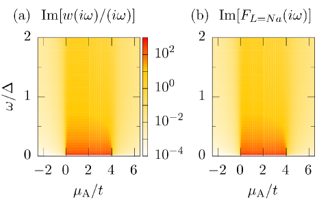
Figure 8: (a) $\mathrm{Im}[w(i\omega)/(i\omega)]$, (b) $\mathrm{Im}[F_{L=Na}(I\omega)]$ with $N=1000$ are plotted as functions of $\mu_{\mathrm{A}}$ and $\omega$ for $\Delta/t=0.1$, $\mu_{\mathrm{B}}/t=1$, $\eta=0.1$ and $\bar{\eta}=0.2$. $\mathrm{Re}[w(i\omega)/(i\omega)]$ and $\mathrm{Re}[F_{L=Na}(i\omega)]$ are zero if $\omega$ is real number. Here the color bar is common for (a) and (b).

Appendix C Spectral bulk-boundary correspondence

The relation between odd-$\omega$ pair amplitudes and the topological number for a chiral symmetric system is given by the spectral bulk-boundary correspondence. Tamura et al. (2019); Daido and Yanase (2019) For chiral symmetric systems, following the spectral bulk-boundary correspondence, we can writeTamura et al. (2019); Daido and Yanase (2019)

$$w(i\omega)/(i\omega)=\lim_{N\rightarrow\infty}F_{L=Na}(i\omega),$$ (39)

with

$$w(i\omega)= \frac{i}{4\pi}\int_{-\pi/a}^{\pi/a}\mathrm{d}k\>\mathrm{tr}\left[\Gamma G(i\omega,k)\partial_{k}G^{-1}(i\omega,k)\right],$$ (40)

$$F_{L=Na}(i\omega)= \sum_{l=1}^{2N}{\left[\gamma g(i\omega)\right]}_{l,l}$$

$$= \sum_{j=1}^{N/2}[g_{4j-3,4j-2}(i\omega)+g_{4j-2,4j-3}(i\omega)$$

$$+g_{4j-2,4j}(i\omega)+g_{4j,4j-2}(i\omega)]$$

$$= \sum_{j=1}^{N/2}\left\{f_{\mathrm{AA}}^{\mathrm{intra}}(i\omega,j)+[f_{\mathrm{AA}}^{\mathrm{intra}}(i\omega,j)]^{\rm T}\right.$$

$$\left.\hskip 22.76219pt+f_{\mathrm{BB}}^{\mathrm{intra}}(i\omega,j)+[f_{\mathrm{BB}}^{\mathrm{intra}}(i\omega,j)]^{\rm T}\right\}$$

$$= 2i\sum_{j=1}^{N/2}\left[f_{\mathrm{AA}}^{\mathrm{OEE}}(i\omega,j)+f_{\mathrm{BB}}^{\mathrm{OEE}}(i\omega,j)\right],$$ (41)

where $\Gamma=\sigma_{0}\tau_{1}$ is the chiral operator for the SC SSH model, $\gamma=\mathrm{diag}(\Gamma,\Gamma,\ldots)$, $w(i\omega)$ is defined in a system with periodic boundary conditions, $F_{L=Na}$ is defined in a system with open boundary conditions, and $f_{\mathrm{AA(BB)}}^{\mathrm{intra}}$ and $f_{\mathrm{AA(BB)}}^{\mathrm{OEE}}$ are given by Eqs. (23) and (17), respectively. In the last line of Eq. (41), we use the fact that all matrix elements of the Hamiltonian in the real space basis is purely real and then the Green’s function satisfies $g^{\rm T}=g$. Note that the components of the Green’s function that are related to $F_{L=Na}(i\omega)$ depend on the chiral operator $\gamma$. Interestingly, the bulk value of $f_{\mathrm{AA}}^{\mathrm{OEE}}(i\omega,j)+f_{\mathrm{BB}}^{\mathrm{OEE}}(i\omega,j)$ is zero due to Eq. (13) with $j=N/2$ is sufficiently far from both edges. This can be seen from the following:

$$\lim_{N\rightarrow\infty}\left[f_{\mathrm{AA}}^{\mathrm{OEE}}(i\omega,j=N/2)+f_{\mathrm{BB}}^{\mathrm{OEE}}(i\omega,j=N/2)\right]$$

$$= \frac{a}{2\pi}\int_{-\pi/a}^{\pi/a}\mathrm{d}k\>\left[F_{\mathrm{AA}}(i\omega,k)+F_{\mathrm{BB}}(i\omega,k)\right]$$

$$= \frac{a}{2\pi}\int_{-\pi/a}^{\pi/a}\mathrm{d}k\>\frac{1}{P(i\omega,k)}\left(\mu_{\mathrm{B}}+\mu_{\mathrm{A}}\right)\left(\Delta_{k}^{*}T_{k}-\Delta_{k}T_{k}^{*}\right)$$

$$= 0,$$ (42)

since $\Delta_{k}^{*}T_{k}-\Delta_{k}T_{k}^{*}=4it\Delta(1-\eta\bar{\eta})\sin(ka)$ is an odd function of $k$. Thus, even though the individual terms $f^{\rm OEE}_{\rm AA}$ and $f^{\rm OEE}_{\rm BB}$ are non-zero in the bulk ($N/2$), the summation of them becomes zero as shown above.

By comparing Eqs. (7) and (40), in the limit $\omega\rightarrow 0$, $w(i\omega)$ reduces to the winding number $W$, namely, $\lim_{\omega\rightarrow 0}w(i\omega)=W$, where $W$ is given by Eq. (7). In Eq. (41), the summation runs from $j=1$ to $j=N/2$ in order to extract the odd-$\omega$ amplitudes bounded close to the surface $j=1$. The reason why the summation is stopped at $N/2$ is that the signs of $f^{\rm OEE}_{\rm AA}+f^{\rm OEE}_{\rm BB}$ are opposite at the left and the right edges. A summation from $j=1$ to $N$ then vanishes. From the definition given by Eq. (41), the total amount of intra-sublattice odd-$\omega$ pairing $f_{\mathrm{AA(BB)}}^{\mathrm{OEE}}$ accumulated close to the surface is connected to the generalized winding number $w(i\omega)$ through Eq. (39).

In order to provide further evidence of the relation between boundary odd-$\omega$ amplitudes and topological number, in Fig. 8(a,b) we present numerical results of $w(i\omega)/(i\omega)$ and $F_{L=1000a}$. We have verified (not shown) that the normalized difference between $w(i\omega)/(i\omega)$ and $F_{L=1000a}$ is smaller than $10^{-9}$. These figures demonstrate that $w(i\omega)/(i\omega)$ and $F_{L=1000a}$ are the same within numerical error. In particular, we can observe that $w(i\omega)/i\omega$ and $F_{L=1000a}(i\omega)$ have large values in the topological phase for small $\omega$. This can be understood as follows. $F_{L=Na}$ is an odd function of $\omega$ and it can be expanded as

$$\lim_{N\rightarrow\infty}F_{N}(i\omega)=W/(i\omega)+i\chi\omega+\mathcal{O}({\omega}^{3})$$ (43)

for small value of $\omega$, where $W$ is the winding number. From Eq. (39), $\chi$ is obtained from the second derivative of $w(i\omega)$ and we can confirm that $\chi$ is a real number. From this expansion, the total amount of the odd-$\omega$ correlations $F_{L=Na}$ diverges in the topological phase ($W\neq 0$) and it is a linear function of $\omega$ in the trivial phase ($W=0$) for small $\omega$. This is summarized in Eq. (25) of the main text.

References

- Berezinskii (1974) V. L. Berezinskii, JETP Lett. 20, 287 (1974).
- Bergeret et al. (2005) F. S. Bergeret, A. F. Volkov, and K. B. Efetov, Rev. Mod. Phys. 77, 1321 (2005).
- Tanaka et al. (2012) Y. Tanaka, M. Sato, and N. Nagaosa, J. Phys. Soc. Jpn. 81, 011013 (2012).
- Linder and Balatsky (2019) J. Linder and A. V. Balatsky, Rev. Mod. Phys. 91, 045005 (2019).
- Cayao et al. (2019) J. Cayao, C. Triola, and A. M. Black-Schaffer, arXiv:1908.05466 (2019).
- Tanaka et al. (2007a) Y. Tanaka, Y. Tanuma, and A. A. Golubov, Phys. Rev. B 76, 054522 (2007a).
- Eschrig et al. (2007) M. Eschrig, T. Löfwander, T. Champel, J. C. Cuevas, J. Kopu, and G. Schön, J. Low Temp. Phys. 147, 457 (2007).
- Golubov et al. (2011) A. A. Golubov, Y. Tanaka, Y. Asano, and Y. Tanuma, Fundamentals of Superconducting Nanoelectronics (Springer Berlin Heidelberg, Berlin, Heidelberg, 2011) pp. 117–131.
- Tanaka et al. (2007b) Y. Tanaka, A. A. Golubov, S. Kashiwaya, and M. Ueda, Phys. Rev. Lett. 99, 037005 (2007b).
- Annunziata et al. (2012) G. Annunziata, D. Manske, and J. Linder, Phys. Rev. B 86, 174514 (2012).
- Higashitani et al. (2009) S. Higashitani, Y. Nagato, and K. Nagai, J. Low Temp. Phys. 155, 83 (2009).
- Tamura and Tanaka (2019) S. Tamura and Y. Tanaka, Phys. Rev. B 99, 184501 (2019).
- Cayao and Black-Schaffer (2018) J. Cayao and A. M. Black-Schaffer, Phys. Rev. B 98, 075425 (2018).
- Ebisu et al. (2016a) H. Ebisu, B. Lu, K. Taguchi, A. A. Golubov, and Y. Tanaka, Phys. Rev. B 93, 024509 (2016a).
- Samokhvalov et al. (2016) A. V. Samokhvalov, A. S. Melnikov, and A. I. Buzdin, Physics-Uspekhi 59, 571 (2016).
- Higashitani (1997) S. Higashitani, Journal of the Physical Society of Japan 66, 2556 (1997), https://doi.org/10.1143/JPSJ.66.2556 .
- Tanaka et al. (2005a) Y. Tanaka, Y. Asano, A. A. Golubov, and S. Kashiwaya, Phys. Rev. B 72, 140503 (2005a).
- Yokoyama et al. (2011) T. Yokoyama, Y. Tanaka, and N. Nagaosa, Phys. Rev. Lett. 106, 246601 (2011).
- Suzuki and Asano (2014) S.-I. Suzuki and Y. Asano, Phys. Rev. B 89, 184508 (2014).
- Suzuki and Asano (2015) S.-I. Suzuki and Y. Asano, Phys. Rev. B 91, 214510 (2015).
- Kashiwaya and Tanaka (2000) S. Kashiwaya and Y. Tanaka, Reports on Progress in Physics 63, 1641 (2000).
- Tanaka and Golubov (2007) Y. Tanaka and A. A. Golubov, Phys. Rev. Lett. 98, 037003 (2007).
- Tanaka and Kashiwaya (2004) Y. Tanaka and S. Kashiwaya, Phys. Rev. B 70, 012507 (2004).
- Tanaka et al. (2005b) Y. Tanaka, S. Kashiwaya, and T. Yokoyama, Phys. Rev. B 71, 094513 (2005b).
- Asano et al. (2006) Y. Asano, Y. Tanaka, and S. Kashiwaya, Phys. Rev. Lett. 96, 097007 (2006).
- Asano et al. (2007) Y. Asano, Y. Tanaka, A. A. Golubov, and S. Kashiwaya, Phys. Rev. Lett. 99, 067005 (2007).
- Hu (1994) C.-R. Hu, Phys. Rev. Lett. 72, 1526 (1994).
- Asano and Tanaka (2013) Y. Asano and Y. Tanaka, Phys. Rev. B 87, 104513 (2013).
- Black-Schaffer and Balatsky (2013a) A. M. Black-Schaffer and A. V. Balatsky, Phys. Rev. B 87, 220506 (2013a).
- Ebisu et al. (2015) H. Ebisu, K. Yada, H. Kasai, and Y. Tanaka, Phys. Rev. B 91, 054518 (2015).
- Ikegaya et al. (2015) S. Ikegaya, Y. Asano, and Y. Tanaka, Phys. Rev. B 91, 174511 (2015).
- Crépin et al. (2015) F. Crépin, P. Burset, and B. Trauzettel, Phys. Rev. B 92, 100507 (2015).
- Huang et al. (2015) Z. Huang, P. Wölfle, and A. V. Balatsky, Phys. Rev. B 92, 121404 (2015).
- Kashuba et al. (2017) O. Kashuba, B. Sothmann, P. Burset, and B. Trauzettel, Phys. Rev. B 95, 174516 (2017).
- Ebisu et al. (2016b) H. Ebisu, B. Lu, J. Klinovaja, and Y. Tanaka, Prog. Theor. Exp. Phys. 2016 (2016b), 083I01.
- Lee et al. (2017) S.-P. Lee, R. M. Lutchyn, and J. Maciejko, Phys. Rev. B 95, 184506 (2017).
- Cayao and Black-Schaffer (2017) J. Cayao and A. M. Black-Schaffer, Phys. Rev. B 96, 155426 (2017).
- Tanaka and Tamura (2018) Y. Tanaka and S. Tamura, J. Low Temp. Phys. 191, 61 (2018).
- Keidel et al. (2018) F. Keidel, P. Burset, and B. Trauzettel, Phys. Rev. B 97, 075408 (2018).
- Fleckenstein et al. (2018) C. Fleckenstein, N. T. Ziani, and B. Trauzettel, Phys. Rev. B 97, 134523 (2018).
- Tsintzis et al. (2019) A. Tsintzis, A. M. Black-Schaffer, and J. Cayao, Phys. Rev. B 100, 115433 (2019).
- Kuzmanovski et al. (2019) D. Kuzmanovski, A. M. Black-Schaffer, and J. Cayao, arXiv:1911.04549 (2019).
- Asano et al. (2011) Y. Asano, A. A. Golubov, Y. V. Fominov, and Y. Tanaka, Phys. Rev. Lett. 107, 087001 (2011).
- Bernardo et al. (2015) A. D. Bernardo, S. Diesch, Y. Gu, J. Linder, G. Divitini, C. Ducati, E. Scheer, M. Blamire, and J. Robinson, Nat. Commun. 6, 8053 (2015).
- Di Bernardo et al. (2015) A. Di Bernardo, Z. Salman, X. L. Wang, M. Amado, M. Egilmez, M. G. Flokstra, A. Suter, S. L. Lee, J. H. Zhao, T. Prokscha, E. Morenzoni, M. G. Blamire, J. Linder, and J. W. A. Robinson, Phys. Rev. X 5, 041021 (2015).
- Black-Schaffer and Balatsky (2013b) A. M. Black-Schaffer and A. V. Balatsky, Phys. Rev. B 88, 104514 (2013b).
- Komendová et al. (2015) L. Komendová, A. V. Balatsky, and A. M. Black-Schaffer, Phys. Rev. B 92, 094517 (2015).
- Asano and Sasaki (2015) Y. Asano and A. Sasaki, Phys. Rev. B 92, 224508 (2015).
- Triola et al. (2020) C. Triola, J. Cayao, and A. M. Black-Schaffer, Annalen der Physik 532, 1900298 (2020).
- Sothmann et al. (2014) B. Sothmann, S. Weiss, M. Governale, and J. König, Phys. Rev. B 90, 220501 (2014).
- Burset et al. (2016) P. Burset, B. Lu, H. Ebisu, Y. Asano, and Y. Tanaka, Phys. Rev. B 93, 201402 (2016).
- Triola and Black-Schaffer (2019) C. Triola and A. M. Black-Schaffer, Phys. Rev. B 100, 024512 (2019).
- Komendová and Black-Schaffer (2017) L. Komendová and A. M. Black-Schaffer, Phys. Rev. Lett. 119, 087001 (2017).
- Triola and Black-Schaffer (2018) C. Triola and A. M. Black-Schaffer, Phys. Rev. B 97, 064505 (2018).
- Kuzmanovski and Black-Schaffer (2017) D. Kuzmanovski and A. M. Black-Schaffer, Phys. Rev. B 96, 174509 (2017).
- Kobiałka et al. (2019) A. Kobiałka, N. Sedlmayr, M. M. Maśka, and T. Domański, arXiv:1909.11550 (2019).
- Aguado (2017) R. Aguado, Riv. del Nuovo Cim. 40, 523 (2017).
- Lutchyn et al. (2018) R. M. Lutchyn, E. P. A. M. Bakkers, L. P. Kouwenhoven, P. Krogstrup, C. M. Marcus, and Y. Oreg, Nat. Rev. Mater. 3, 52 (2018).
- Culcer et al. (2020) D. Culcer, A. C. Keser, Y. Li, and G. Tkachov, 2D Materials 7, 022007 (2020).
- Su et al. (1979) W. P. Su, J. R. Schrieffer, and A. J. Heeger, Phys. Rev. Lett. 42, 1698 (1979).
- Su et al. (1980) W. P. Su, J. R. Schrieffer, and A. J. Heeger, Phys. Rev. B 22, 2099 (1980).
- Asbóth et al. (2016) J. K. Asbóth, L. Oroszlány, and A. Pályi, Lecture notes in physics 919, 87 (2016).
- Wakatsuki et al. (2014) R. Wakatsuki, M. Ezawa, Y. Tanaka, and N. Nagaosa, Phys. Rev. B 90, 014505 (2014).
- Sticlet et al. (2014) D. Sticlet, L. Seabra, F. Pollmann, and J. Cayssol, Phys. Rev. B 89, 115430 (2014).
- Zhang et al. (2019) H. Zhang, D. E. Liu, M. Wimmer, and L. P. Kouwenhoven, Nat. commun. 10, 1 (2019).
- Tamura et al. (2019) S. Tamura, S. Hoshino, and Y. Tanaka, Phys. Rev. B 99, 184512 (2019).
- Daido and Yanase (2019) A. Daido and Y. Yanase, Phys. Rev. B 100, 174512 (2019).
- Deutschmann et al. (2001) R. A. Deutschmann, W. Wegscheider, M. Rother, M. Bichler, G. Abstreiter, C. Albrecht, and J. H. Smet, Phys. Rev. Lett. 86, 1857 (2001).
- Gangadharaiah et al. (2012) S. Gangadharaiah, L. Trifunovic, and D. Loss, Phys. Rev. Lett. 108, 136803 (2012).
- Ezawa et al. (2013) M. Ezawa, Y. Tanaka, and N. Nagaosa, Sci. Rep. 3, 2790 (2013).
- Szumniak et al. (2019) P. Szumniak, D. Loss, and J. Klinovaja, arXiv:1910.05090 (2019).
- Ramires et al. (2018) A. Ramires, D. F. Agterberg, and M. Sigrist, Phys. Rev. B 98, 024501 (2018).
- Ramires and Sigrist (2019) A. Ramires and M. Sigrist, Phys. Rev. B 100, 104501 (2019).
- Sato et al. (2011) M. Sato, Y. Tanaka, K. Yada, and T. Yokoyama, Phys. Rev. B 83, 224511 (2011).
- Takagi et al. (2020) D. Takagi, S. Tamura, and Y. Tanaka, Phys. Rev. B 101, 024509 (2020).
- Pivovarov and Nayak (2001) E. Pivovarov and C. Nayak, Phys. Rev. B 64, 035107 (2001).
- Kedem and Balatsky (2015) Y. Kedem and A. V. Balatsky, arXiv:1501.07049 (2015).