Spectral Signatures of Quasar Ages at ${\emph{z}\approx 3}$

Abstract

Insight into quasar ages may be obtained from the proximity effect, but so far only in a limited number of bright quasars. Based on $\sim 2600$ SDSS quasar spectra at $2.5\leq z\leq 3.5$, a search for spectral voids between Ly$\alpha$ forest lines finds proximity zones over a wide range of radial distances. The majority of zone sizes are less than 5 Mpc, with their numbers decreasing exponentially towards larger distances. After normalization by luminosities, the zone sizes are distributed with an e-folding scale of 0.64 as compared with the anticipated values. A group of quasars are selected for their large proximity zones of $\gtrsim 10$ Mpc. Their composite spectrum displays strong narrow cores and large equivalent widths in Ly$\alpha$ and other major UV emission lines. If the proximity zones along lines of sight are indicative of quasar ages, these features may be the signatures of old quasars. Another group of quasars are selected as they show no proximity zone and exhibit intrinsic absorption lines at $z_{ab}>z_{em}$. They are likely young quasars and exhibit weaker narrow emission-line components. The significant difference of spectral features between the two groups may reflect an evolution pattern over quasars’ lifetimes.

1 INTRODUCTION

What is a quasar’s lifetime? How do quasars evolve over their lifetimes? To answer these questions regarding supermassive black holes, it is essential to find clues to the age of quasars. However, such time tags are scarce as quasar spectra, unlike those of stars and galaxies, consist of power-law segments that extend to high frequencies (Elvis et al., 1994; Shang et al., 2011). While the UV bumps are believed to be related to the accretion disks, the estimates of their temperatures are difficult (Blackburne et al., 2011). Various methods have been tried to probe quasar ages, but the results are uncertain and sometimes inconsistent, with a possible range between $1-100$ Myr (Martini, 2004; Kirkman & Tytler, 2008; DiPompeo et al., 2014).

Perhaps the best trace for a quasar’s age is in its vicinity. The enormous UV radiation of quasars produces cosmic bubbles of high ionization that expand and eventually overlap. The accumulated ionizing radiation field, commonly referred to as the metagalactic UV background (UVB) radiation, completed the reionization of the intergalactic medium (IGM; Meiksin, 2009; McQuinn, 2016) at $z\approx 3$. The trace of high-ionization zones around quasars can be found in their spectra as the line-of-sight proximity effect (Carswell et al., 1982; Murdoch et al., 1986; Bajtlik et al., 1988). In the hydrogen Ly$\alpha$ forest lines at $z\approx 3$, the effect is observed as a decrease in the number of forest absorption lines. In the helium Ly$\alpha$ spectra at $z\approx 3$, the opacity is large enough that a continuous proximity profile may be present (Zheng & Davidsen, 1995). The helium proximity profiles in a few dozens of quasars (Zheng et al., 2015; Khrykin et al., 2016, 2019; Zheng et al., 2019) have been used to estimate quasar ages.

Early studies of the proximity effect were carried out with high-resolution optical spectra where a large number of absorption lines could be identified (Carswell et al., 1987; Giallongo et al., 1996; Lu et al., 1996; Cooke et al., 1997). Later studies (Bechtold, 1994; Scott et al., 2000; Liske & Williger, 2001; Guimarães et al., 2007) often used spectra of medium resolution of $\sim 4000$ to find a deficiency of absorption lines near the quasar redshifts and derive the UVB intensity. Dall’Aglio et al. (2008a) used high signal-to-noise (S/N), low-resolution ($R\approx 800$) spectra to carry out such a study. The largest sample size among these studies is 45 (Guimarães et al., 2007).

The proximity effect can also be studied along the transverse direction if a bright foreground quasar is present near the line of sight towards another distant quasar (Dobrzycki & Bechtold, 1991). Most H I studies in the optical band have not yielded significant detections (Liske & Williger, 2001; Kirkman & Tytler, 2008; Lau et al., 2016), but He II studies have made several estimates of quasar ages of up to $\sim 34$ Myr (Jakobsen et al., 2003; Syphers & Shull, 2014; Schmidt et al., 2017, 2018).

The Sloan Digital Sky Survey (SDSS; York et al., 2000), its follow-up SDSS-II Supernova Survey (Friedman et al., 2008), SDSS-III/BOSS (Eisenstein et al., 2011), and SDSS-IV/eBOSS (Blanton et al., 2017) have revolutionized the way we study quasars. Over the last two decades, the number of known quasars has increased dramatically from several thousand to approximately half a million (Schneider et al., 2010; Pâris et al., 2014, 2017, 2018). This paper describes an analysis of medium-resolution SDSS spectra in search of the proximity effect. It is known that some quasars display small proximity zones: for He II zones at $z\approx 3$ (Shull et al., 2010; Zheng et al., 2015; Khrykin et al., 2016) and H I zones at $z\approx 6$ (Eilers et al., 2018). Does such a trend exist for H I zones at $z\approx 3$? The significant sample size enables one to derive the distribution of proximity-zone sizes and to identify groups of both old and young quasars.

2 DATA ANALYSES

Quasar spectra at $2.5\leq z\leq 3.5$ and with a limiting magnitude of 19 in the $i^{\prime}$ band were retrieved from the Data Releases 7, 10, and 12 (DR, Abazajian et al., 2009; Ahn et al., 2014; Alam et al., 2015, respectively). Figure 1 displays the distribution of these 3298 quasars. SDSS spectra cover a wavelength range $\sim 3600-10500$ Å, at a resolution of $\sim 2000$. The data at the red and blue ends are of low S/N ratio, therefore, the nominal spectra range is $\sim 3800-9200$ Å. At redshifts of 2.5 and higher, the Ly$\alpha$ emission moves into the region of $\lambda>4255$ Å, securing a spectral window $\Delta\lambda\gtrsim 450$ Å with reasonable S/N ratios for the study of forest absorption. The upper limit of $z=3.5$ is set to secure the C III] $\lambda 1909$ (C III] hereafter) emission line well below 9000 Å to avoid significant night-sky lines. The average redshift of this sample is $z=2.84\pm 0.26$ with a median of 2.78. The spectra were processed in units of vacuum wavelength. When multiple spectra exist for a given quasar, they were merged with the weights of S/N ratios. All the wavelengths and equivalent widths (EW) are in the rest frame, and all distances as proper distances hereafter. At $z\approx 3$, the distance scale is approximately 0.8 Mpc per Å.

2.1 Simulations of Ly$\alpha$ Forest Lines

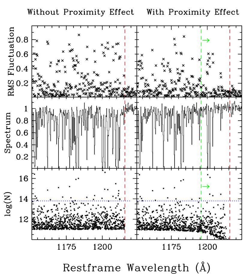
Figure 2: Simulations of Ly$\alpha$ forest lines at $z=3$. The left panels show the original properties without the proximity effect, and the right panels with a proximity zone of $R_{\omega=1}=20$ Å, as marked with a green dashed line and arrows. The red dashed lines mark the Ly$\alpha$ wavelength. The lower panels are the column density $N$ of simulated absorbers, in units of $\rm cm^{-2}$, the middle panels the forest spectra, and the upper panels the RMS-fluctuation spectra. The spectral voids near Ly$\alpha$ in the right panels are associated with absorbers of column density $\log N\lesssim 13.8$ $\rm cm^{-2}$ below the blue dotted line.

To check the feasibility of finding the proximity effect with SDSS spectra, Ly$\alpha$ forest-line spectra were simulated at $z\approx 3$. Following an empirical power-law distribution of column densities $dn/dN\propto N^{-1.5}$ (Tytler, 1987), absorbers were generated between column densities of $\log N=11-17$ $\rm cm^{-2}$ and $\lambda=1050-1216$ Å. The wavelengths of these absorbers are random but follow a distribution of $dn/dz\propto(1+z)^{2.5}$ (Janknecht et al., 2006). For every absorber, a Voigt profile of Doppler parameter $b=30$ ${\rm km\,s}^{-1}$ was produced on a flat continuum over a grid of 0.01 Å scale. Over the range of $1050-1170$ Å, there are $\sim 2700$ lines, among which $\sim 67$ are at $\log N>13.5$ $\rm cm^{-2}$. The spectra were then binned to match the SDSS resolution with added noise at an S/N ratio of 20. The left panels of Figure 2 display an example of simulated data: the column densities of absorbers, the normalized forest-line spectrum and the RMS-fluctuation spectrum (absolute values of the flux difference between adjacent pixels). The effective optical depth produced by all Ly$\alpha$ absorption may be expressed as $\tau=0.0021\ (1+z)^{3.7}$ (Meiksin, 2006), and the simulations found that weak absorbers of column density $\log N\lesssim 13.4$ $\rm cm^{-2}$ contribute approximately a half of this opacity.

The proximity effect is commonly characterized by the ratio of the local quasar flux to that of the UVB, $\omega=F_{Q}/(4\pi J_{\nu})$, where $J_{\nu}$ is the angle-averaged specific intensity (Bajtlik et al., 1988). For the UVB intensity $\log J_{\nu}\simeq-21.5$ ${\rm erg\,cm}^{-2}\,{\rm s}^{-1}\,{\rm Hz}^{-1}{\rm Sr}^{-1}$  (Dall’Aglio et al., 2008b; Bolton et al., 2005), the proximity zones of $\omega\approx 1$ are moderate, on the order of 5 Mpc. In the right panels of Figure 2, the properties of a large proximity zone with $R_{\omega=1}=20$ Å ($\approx 16$ Mpc) are plotted.

Most Ly$\alpha$ absorption lines that can be identified in SDSS spectra are saturated. Their strengths are therefore insensitive to the proximity effect, and few vanish in the quasar vicinity. A significant effect is on the weak components at $\log N\lesssim 13.8$ $\rm cm^{-2}$ (EW $\lesssim 0.1$ Å). They are located on the linear part of the curve of growth, and their strengths are proportional to changing column densities. While these weak absorption features cannot be individually identified at medium resolutions, their combined proximity effects are spectral voids between strong absorption lines, as shown in the right panels of Figure 2. Given the limited resolution and S/N ratios of SDSS spectra, the spectral voids in the forest-line region are used in this study as a signature of the proximity effect.

2.2 RMS Fluctuation Spectra

In a process of flux normalization, absorption lines in the SDSS spectra were first identified using local flux troughs. By making the flux differences between adjacent pixels in a spectrum, an array of first-order derivative was made, and then was a second-order derivative by repeating the same method to the latter. After a local trough was identified from the second-order derivative, a “climbing” process started towards both the longer and shorter wavelengths until nearby “plateaus” were found, which marked the endpoints of this absorption feature. The EW and statistical significance were calculated, and the corresponding wavelength window of this absorption feature was flagged out. The weakest features that could be identified were of EW $\approx 0.15$ Å. The fitting task Specfit (Kriss, 1994) was carried out over several wavelength ranges. The algorithm allows a variety of input components with free parameters, including a power-law continuum, Gaussian and Lorentzian emission lines, Gaussian absorption lines, and user-supplied components. During the analysis of a quasar spectrum, it first fit the wavelength region of $1216-1950$ Å, excluding the spectral windows of identified absorption features. The components included a power-law continuum, Gaussian emission lines for Ly$\alpha$, N V $\lambda 1240$, C IV $\lambda 1549$, and C III]. Secondly, it fit the wavelength region of $1150-1270$ Å for improved normalization near and below the Ly$\alpha$ wavelength. In the forest-line region, only a small fraction of pixels are free of absorption features. These high-flux points were included in the fitting windows. At medium spectral resolutions, even these high points are below the flux extrapolation of a power law from longer wavelengths because of unresolved forest absorption lines. To mitigate this effect, a set of five “userabs” files with index keys were made in two columns: wavelength and optical depth. They represent a smooth attenuation component with $\tau=k\ 0.001\ (1+z)^{3.7}\ P$, where the coefficient 0.001 represents the effective optical depth of unresolved weak Ly$\alpha$ forest lines (approximately a half of the total), the normalization factor $k$ between 0.0 and 1.0, and $P=(1+(R_{\omega=1}/R)^{2})^{-1}$ the proximity term. Fixed characteristic distances $R_{\omega=1}$ of 2.5, 5, 10, 15, and 20 Å were assigned to these files, respectively, and radial distances from the quasar, $R$, were calculated as a function of wavelengths. This user-supplied component applied attenuation to all the pixels in the forest-line region. Its free parameters were the index key of input files ($1-5$) and the normalization scale of optical depth, $k$. The fitting process yielded the best values of these two parameters, but their associated errors were large in many cases. The narrow components of emission lines were tied to that of Ly$\alpha$ at FWHM (Full Width at Half Maximum) $\leq 2500$ ${\rm km\,s}^{-1}$, and their broad counterparts tied to that of Ly$\alpha$ at FWHM$>2500$ ${\rm km\,s}^{-1}$. After these fitting steps, a normalized spectrum was produced for each quasar, with absorption-line windows flagged out.

A prominent difference between the forest-line region and the rest of a quasar spectrum is their RMS characteristics. An RMS-fluctuation spectrum is made of the absolute values of flux difference between adjacent pixels in a normalized spectrum, after slight smoothing. As shown in Figure 2, the fluctuation properties are visibly different across the Ly$\alpha$ wavelength. They provide a sensitive probe of spectral voids, and are largely unaffected by the flux normalization.

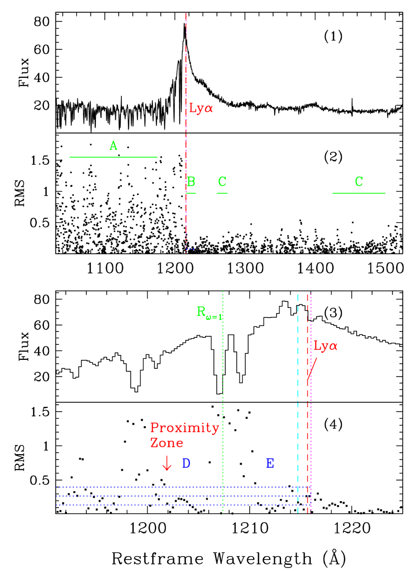
Figure 3: Spectrum of quasar SDSS1438+0831, $z=2.839$, and its RMS fluctuations. The flux unit is $10^{-17}$ ${\rm erg\,s}^{-1}\,{\rm cm}^{-2}\,{\rm\AA}^{-1}$, and the RMS spectra are smoothed by 3 pixels. In panel 2, the average value in region A is 0.40, and $0.074\pm 0.057$ in region B, yielding $\zeta\approx 5.4$. Region C is marked but not used. In panels 3 and 4, the Ly$\alpha$ wavelength is marked in red, that for the PCA redshift in magenta dots, that for the C III] redshift in cyan, and the characteristic distance of $R_{\omega=1}$ in green. Three blue horizontal dotted lines represent the levels of $t=0.2$, 0.6, and 1.0, respectively, from low to high. There are two voids, D and E, and the proximity-zone size is marked with a downward arrow at the left boundary of D.

A statistical analysis was carried out on RMS-fluctuation spectra in three regions: (A) the forest-line region between $1050-1175$ Å, which is largely free of the proximity effect, (B) Ly$\alpha$ emission-line region between $1216-1230$ Å, and (C) two “clean” regions of $1260-1275$ and $1425-1500$ Å. In the region A, all pixels were included, and in the region B and C, the wavelength windows with identified absorption features were excluded. The contrast parameter is defined as $\zeta=(\bar{A}-\bar{B})/\sigma(B)$, where $\bar{A}$ and $\bar{B}$ are mean fluxes in the A and B regions, respectively, and $\sigma(B)$ the standard deviation of fluxes in the B region. This ratio reflects the significance of the forest signature: a null $\zeta$ value would imply no difference in fluctuation characters between regions A and B. Figure 3 illustrates the fitting windows and the effect of parameters in a typical quasar. In rare cases ($\sim 4.6\%$ of the whole sample), spectral region B was affected by many absorption features, and a better contrast ratio between regions A and C was used. Since the potential proximity zone and regions B are at higher fluxes than the continuum level, the average and standard deviation derived from region C were scaled by the square foot of the ratio of fitted fluxes between regions C and B. Tests made for the other quasars confirmed that such estimates between regions B and C were consistent with 20%.

In general, the $\zeta$ value increases with heavier smoothing, but individual spectral features become less visible. It appears that a smoothing box of 3 pixels is proper in finding spectral voids. A small fraction of quasars shows low S/N ($<3$) or contrast ratios ($\zeta<1.3$). They were excluded in this study because of high uncertainties in determining their proximity zones.

2.3 Systemic Redshifts

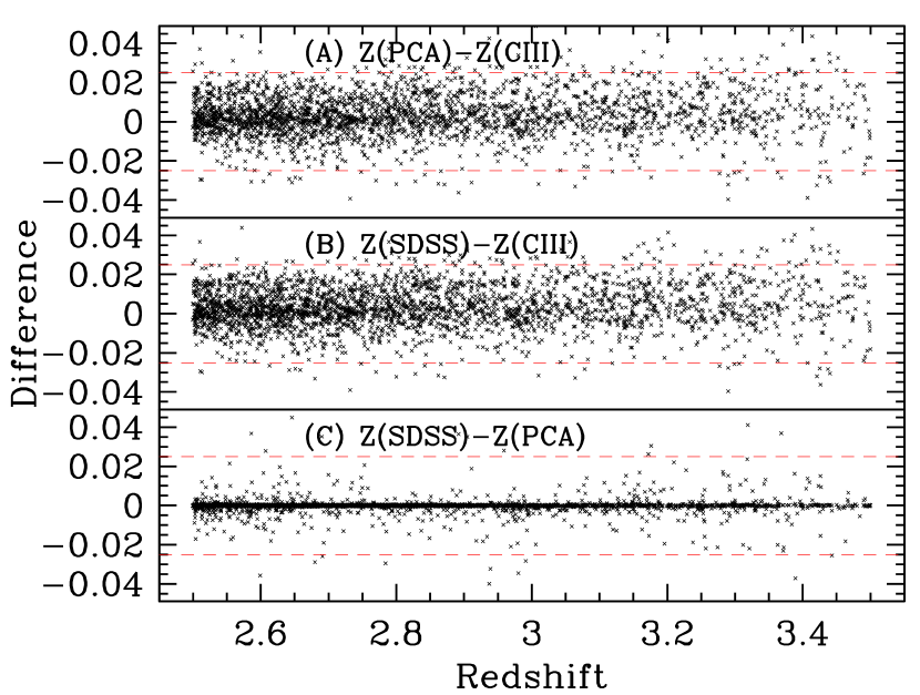
Figure 4: Redshift differences between the three sets of SDSS measurements. Panel A: between the PCA redshifts and the C III] redshifts; panel B: between SDSS pipeline redshifts, and C III] redshifts, with $z(SDSS)-z(C_{III})=0.0023\pm 0.0094$; and panel C: between the SDSS pipeline redshifts, and PCA redshifts. Objects beyond the range $-0.025<dz<0.025$, as marked with red dashed lines, are not used in the study.

Accurate quasar redshifts set the zero points of proximity zones and hence are essential in understanding the level of uncertainties. However, this issue remains controversial as emission lines display slightly different redshifts. The SDSS pipeline provides its best redshift estimates from multiple emission lines in quasar spectra, which are referred to as the SDSS redshifts. Hewett & Wild (2010) derived the redshifts of SDSS quasars independently and found a systematic difference as a function of redshift. They suggested that, at $z\approx 3$, C III] may serve as a good reference line. The SDSS spectra after DR 7 provide additional information, including the PCA (Principal Component Analysis) redshifts and C III] redshifts. As shown in Figure 4, the difference between PCA and pipeline redshifts are small: $z(SDSS)-z(PCA)=-0.0010\pm 0.0053$. The differences for C III] redshifts show larger dispersion: $z(PCA)-z(C_{III})=0.0039\pm 0.0092$, and $z(SDSS)-z(C_{III})=0.0023\pm 0.0094$. Nearly 90% of the candidates have tabulated C III] redshifts from the SDSS pipeline. For other quasars that were processed in DR 7, The Specfit fitting task was carried out in the wavelength region of $1800-1950$ Å, excluding the spectral windows of significant night sky and absorption lines. The underlying continuum was assumed as a power law, and four Gaussian components were used: Al III $\lambda 1857$, Si III] $\lambda 1892$, and a pair of narrow and broad C III] lines. The C III] redshifts were derived from the centroids of the fitted narrow C III] components. When the flux of a narrow C III] component was less than 20% of the broad counterpart, another round of fitting was made with a single Gaussian component to determine the C III] centroid.

The objects with differences $dz>0.025$ or $dz<-0.025$ between any pair of the three redshift values were rejected as they are beyond the $2\sigma$ range and may cause considerable uncertainties. The average difference is $z_{SDSS}-z_{CIII}=0.0037\pm 0.0116$ for the samples. If the C III] redshifts are used, there would be a systematic shift of Ly$\alpha$ peak by $-1\pm 3$ Å.

2.4 Measurement of Proximity Zone

As discussed above, some quasar spectra were excluded because of their low quality or unusually large uncertainty in their redshifts. In addition, the spectra that display broad absorption lines, which account for approximately 12% of the sample, were also excluded. Broad absorption lines make large voids in the RMS-fluctuation spectra that resemble proximity zones. Absorption lines in the data are considered “broad” if their EW are larger than $5$ Å between $1175-1250$ Å, or larger than $10$ Å between $1050-1175$ Å. All the spectra were visually inspected, and a few spectra with significant artifacts such as flux spikes were excluded. Overall, the final sample consists of 2594 quasars.

Searches for proximity zones were carried out from 1216 Å (the origin) towards shorter wavelengths, based on the presence of spectral voids of 3.5 Å or larger in RMS-fluctuation spectra. The task started from the points below a threshold of $\bar{B}+t_{0}\zeta\sigma(B)$, where $t_{0}=0.2$. it then moved towards nearby high points until it hit a threshold $\bar{B}+t_{1}\zeta\sigma(B)$, where $t_{1}=0.6$. The separation between the two endpoints was taken as the void size. If a void was 3.5 Å or larger, it was tentatively selected. In the cases of multiple voids in a quasar’s vicinity, the shortest wavelength of the furthest void was taken to mark the size of its proximity zone. The choice of zone-size limit and threshold parameters $t_{0}$ and $t_{1}$ affects the estimates of proximity-zone sizes, and these parameters were optimized over test runs so that the variations of zone sizes are the least sensitive to them. For example, for $t_{1}$ increased from 0.6 to 0.7, the average zone size of the whole sample becomes smaller by 7%. If it is increased to 0.8, the corresponding change in zone size is 17%. In panel 4 of Figure 3, two spectral voids are found within the radial distance of $2R_{\omega=1}$: D ($\sim 1202-1206$ Å) and E ($\sim 1210.5-1214$ Å). Three levels of $t$ values, 0.2, 0.6, and 1.0, are marked from low to high. Since the boundaries of most voids are steep, the $t$ values do not affect the void sizes significantly.

The distribution of proximity-zone sizes is plotted in Figure 5. The bin with the largest number of proximity-zone sizes is at $0-5$ Mpc, and the numbers decline towards larger distances exponentially with a correlation coefficient $r=-0.99$ between $R$ and $\log(N)$ and an e-folding distance of 3.6 Mpc. Since proximity zones are dependent on quasar luminosities, it is useful to normalize the zone sizes by quasar luminosities. Characteristic sizes, $R_{\omega=1}$, were calculated from the $i^{\prime}$-band magnitude and nominal optical-UV and extreme-UV (EUV) spectral shapes. They serve only as a coarse scale because the quasar’s ionizing continuum is extrapolated using an average EUV power law (Zheng et al., 1997; Telfer et al., 2002), and the UVB is fluctuating (Meiksin & McQuinn, 2019). The normalized proximity-zone sizes, namely the ratios of measured to characteristic values, also distribute exponentially ($r=-0.99$) with an e-folding scale of 0.64.

3 RESULTS

3.1 Quasars with Large Proximity Zone

A group of quasars is selected for their large proximity zones, based on the following criteria: (1) a spectral void that starts (at its longest wavelength) between 1.0 and 2.0 $R_{\omega=1}$ and with a size of $\geq 3.5$ Å, (2) a minimum zone size of 10 Mpc, as measured at the ending (the shortest) wavelength, and (3) no absorption lines at $z_{ab}>z_{em}$. Ninety-two quasars ($\sim 4$ % of the sample) match these criteria. They are potentially old quasars because of their large ionized zones, but see §4.1 for more justifications.

A composite spectrum with a pixel scale of 1.0 Å was generated for this group. All spectra were first normalized around 1350 Å. For every merging spectrum, the pixels that fall into the absorption windows were flagged and excluded. Within 20 Å from the Ly$\alpha$ wavelength, these flagged data points were filled with fitted values (see §2.2). Every data point in the composite spectrum took the median of the fluxes of merging spectra at this wavelength. As shown in the lower panel of Figure 6, the spectrum of this group shows strong narrow components in major emission lines, most notably Ly$\alpha$. Several other combining algorithms were also tried, such as an equal weight for every source and an average value at each wavelength bin. While the resultant spectra differ in details, a strong narrow Ly$\alpha$ core is always present.

3.2 Quasars with Infalling System and No Proximity Zone

Since approximately half of the quasars in the sample display small or no proximity zones, it is necessary to find a subgroup among them that is most representative of young quasars. It is noted that some quasars in this sample display narrow absorption features on the red wing of Ly$\alpha$ emission lines, and nearly all them ($>95$%) exhibit no proximity zones. Another group is therefore selected based on the lack of proximity zones (no spectral voids of $\geq 3.5$ Å and no voids of $\geq 2$ Å within 3.5 Å from Ly$\alpha$) and the presence of infalling systems at $z_{ab}>z_{em}$: (1) The absorption redshift is larger than any of the tabulated Ly$\alpha$ redshifts $-$ the SDSS pipeline redshift, C III] redshift and PCA redshift. The longest Ly$\alpha$ wavelength among these three is considered as the lower end of the selection window, which extends to 1226 Å. (2) Only significant absorption features with EW $>0.5$ Å are selected. (3) Potential doublets of metal absorption, including N V $\lambda 1240$, C IV $\lambda 1549$, and Mg II $\lambda 2799$, are rejected. These features are flagged when their wavelength separations are within 0.5 Å from the expected theoretical values, their intensity ratios within 35% of the theoretical value ($0.5-1.0$).

These 77 objects, which account for approximately 3% of the sample, are characterized by weak narrow cores of emission lines. While it is possible that strong absorption features near the Ly$\alpha$ wavelength may hinder the narrow Ly$\alpha$ core, the effect is mitigated using the fitted values in these flagged data points of each spectrum.

The upper panel of Figure 6 shows the composite spectrum for this group of potentially young quasars. The most significant feature for these young quasars is the weak narrow core in Ly$\alpha$. In the middle panel, the composite spectrum for all the quasars in this sample is plotted.

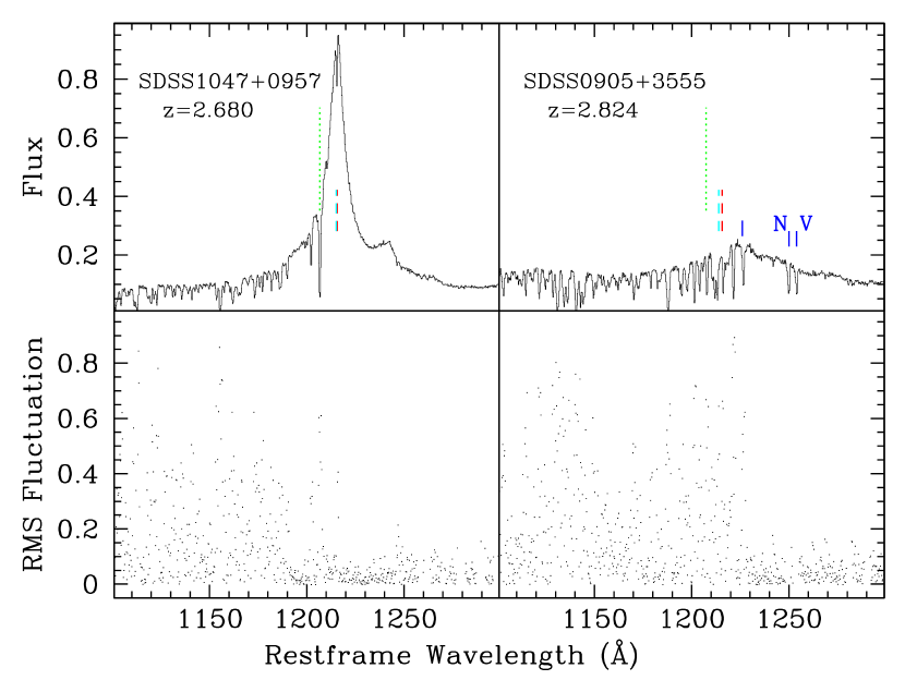
Figure 7: Spectra of two distinct quasars and their RMS-fluctuations. Top left panel: a spectrum with a large proximity zone down to $\sim 1192$ Å. Top right panels: another spectrum with no proximity zone. A pair of N V $\lambda\lambda 1238/1242$ and associated Ly$\alpha$ absorption lines are marked in blue as an infalling system at $z_{ab}=2.858$. Red and cyan bars mark the Ly$\alpha$ wavelengths derived from the SDSS redshifts, which are identical to the PCA values in most cases, and the C III] redshifts, respectively. The long green dotted lines mark the respective characteristic zones $R_{\omega=1}$. The two spectra are scaled so that their fluxes are equal around 1300 Å. The two RMS-fluctuation spectra are roughly normalized.

To demonstrate the sharp difference in emission-line profiles, Figure 7 displays the spectra of two individual quasars from these groups, along with their RMS fluctuations. The quasar spectrum in the top left panel displays a strong narrow Ly$\alpha$ component. In the lower left panel, several spectral voids suggest a proximity zone as large as 24 Å ($\sim 20$ Mpc). In the top right panel, another quasar spectrum displays a broad Ly$\alpha$ profile and no proximity zone.

3.3 Comparison of Spectral Properties

The Specfit task was carried out for the three composite spectra of young quasars, old quasars, and the full sample. The fitting components included a broken power law, Gaussian profiles for emission lines and a set of smooth absorption profile with different optical depths shortward of the Ly$\alpha$ wavelength. For strong emission lines, dual components were used: A narrow Gaussian of FWHM$\sim 2300$ ${\rm km\,s}^{-1}$, and a broad one of $\sim 11000$ ${\rm km\,s}^{-1}$. The widths for O VI $\lambda 1035$, N V $\lambda 1240$, C IV $\lambda 1549$, and C III] components were tied to those of Ly$\alpha$. For weak lines of O I $\lambda 1304$, C II $\lambda 1335$, and Si IV $\lambda 1402$, single Gaussian components were used. As shown in Table 1, the main difference between the young and old quasars are the EW of narrow-line components, with the EW of narrow Ly$\alpha$ varying by a factor of ten. The EW of broad components are similar in all three groups, with relative differences of $\lesssim 30\%$. Table 2 lists the FWHM of the fitted emission lines.

The UV continua of young quasars appear slightly redder than the old ones. The breaking wavelength for the dual power-law components is near Ly$\alpha$, and the average power-law indices ($f_{\lambda}\propto\lambda^{-\beta}$) at wavelengths longward of Ly$\alpha$ are $\beta=1.24\pm 0.37$ for young quasars, $1.46\pm 0.32$ for old quasars and $1.38\pm 0.41$ for the whole sample. The fitting results of the composite spectra yield $\beta=1.22\pm 0.01$ for the young quasars, $1.56\pm 0.02$ for the old ones, and $1.47\pm 0.01$ for the whole sample.

The three groups have similar luminosities: the average absolute magnitudes are $-27.79\pm 0.39$ for the young quasars, $-27.82\pm 0.41$ for the old quasars, and $-27.81\pm 0.44$ for the whole sample. The average redshift for the young quasars is $2.86\pm 0.29$, slightly higher than that of the old quasars ($2.80\pm 0.26$). The observed difference in emission lines likely reflects an evolution trend over a quasar’s lifetime instead of a luminosity or redshift effect.

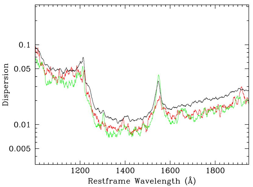
Figure 8: Dispersion spectra as a fraction of the respective composite spectra. Black curve: all quasars; red curve: young quasars, and green curve old quasars.

To estimate the sample dispersion, 100 composite spectra were generated by randomly selecting subgroups of 50 quasars from a parent sample. A dispersion spectrum was generated by taking the standard deviations at each wavelength bin. As shown in Figure 8, the intrinsic dispersions are similar for different groups, with larger dispersion at emission-line regions and the Ly$\alpha$ forest region.

4 DISCUSSION

4.1 Effect of Light Travel Time

The observed expansion of H I proximity zones along lines of sight is believed to be superluminal because an ionizing front propagates at nearly the speed of light in the quasar vicinity (White et al., 2003). Several IGM models assumed an infinite speed for the line-of-sight development of a proximity zone (Bolton & Haehnelt, 2007; Lu & Yu, 2011; Khrykin et al., 2016), thus ruling out the possibility of using the H I proximity effect to scale quasar ages. This hypothesis can be tested with He II proximity profiles, as their development should display significant lags with respect to their H I counterparts. Zheng et al. (2019) studied the He II and H I proximity zones in 15 quasars and found a significant correlation between them. Since the sizes of He II proximity zones are believed to be related to quasar ages (Khrykin et al., 2016, 2019), the H I zone sizes should also bear the signature of quasar ages. The correlation between the sizes of He II and H I proximity zones suggests that the expansion of quasar ionizing fronts may be noticeably slower than the speed of light. One possibility is that quasar activities are episodic on a time scale of the IGM’s equilibration ($\approx 10^{4}$ yr). While more work is needed to explain this observed trend, the relation may serve as an empirical gauge to probe young and old quasars from the sizes of their H I proximity zones.

4.2 Effect of External Sources

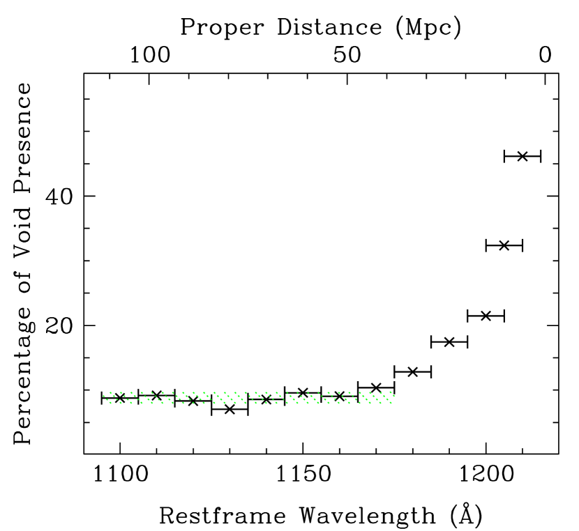
Figure 9: Number of spectral voids of size 3.5 Å or larger in the rest frame. The search is carried out in the RMS-fluctuation spectra of 2594 quasars. The green shaded region marks the $1\sigma$ confidence range for the results between 1095 and 1175 Å. The top labels mark the distances to a quasar at $z=2.8$. The proximity effect is present beyond $10\sigma$ at wavelengths longer than 1190 Å, or radial distances up to $\sim 20$ Mpc.

Quasar sightlines pass through a vast volume of the IGM, whose properties are subject to significant variations. The forest-line spectra of some quasars display significant voids (Dobrzycki & Bechtold, 1991; Syphers & Shull, 2014), which are believed to be the IGM clustering properties or the transverse proximity effect due to the foreground quasars near sightlines. To test the level of contamination by external sources, the distribution of spectral voids is studied at different wavelengths. As shown in Table 3 and Figure 9, the majority of quasars display spectral voids of 3.5 Å and larger. The probability of finding such voids at wavelengths below 1170 Å is $8.8\pm 0.9\%$ per interval of 10 Å. This percentage increases significantly to $\sim 46\%$ in the wavelength range of $1205-1215$ Å, providing evidence that the majority of voids in the quasar vicinity are associated with the intrinsic proximity effect. The contamination rate is estimated at approximately 20%, but the actual rate is lower as the voids with their RMS-fluctuation troughs lower than those at longer wavelengths, a common feature for external spectral voids, were rejected.

4.3 Effect of Overdensity

It is common to assume that the dark matter in the quasar vicinity is denser than the IGM’s average, as quasars are believed to be associated with the most massive galaxies (Kauffmann & Haehnelt, 2000; Springel et al., 2005). The net effect for a higher density is a higher number of absorbers and smaller proximity zones. Guimarães et al. (2007) found that the mean overdensity is of the order of two and five within, respectively, 10 and 3 Mpc from a quasar. At such levels of overdensity, the characteristic sizes would be reduced modestly, but most proximity zones would not be dramatically reduced or masked. It would be ever harder to explain the proximity zones larger than 10 Mpc in terms of underdensity, as the IGM density would have to be lower by a factor of $\sim 4-10$ in a large volume along these lines of sight.

4.4 Effect of Viewing Angles

The differences in line profiles between the young and old quasars bear resemblance to that between the Type-I and II active galactic nuclei (AGNs). The narrow Ly$\alpha$ cores in the group of old quasars are of FWHM $\approx 1500-3500$ ${\rm km\,s}^{-1}$. As a comparison, nearly all the Type-II SDSS quasars display line widths FWHM(H$\beta$)$<1500$ ${\rm km\,s}^{-1}$ (Zakamska et al., 2003), and a new study has set an upper limit of 1000 ${\rm km\,s}^{-1}$ (Yuan et al., 2016). These Ly$\alpha$ emission profiles also display significant broad wings; therefore, the sample consists of Type-I quasars only. But would it be possible that the observed differences are attributed to viewing angles?

Quasar radiation is believed to be highly anisotropic, therefore, the surrounding proximity zone is not spherical. According to the unification theory of AGN (Urry & Padovani, 1995), Type-I AGN display broad emission lines as they are viewed at head-on directions towards obscuring tori. Viewing angles affect the observed broad-line widths and EW (Rudge & Raine, 1997). The quasar radiation is expected to be strong at such viewing angles, therefore, larger proximity zones and broader emission lines are anticipated. This seems inconsistent with the results shown in Figure 6.

Fine et al. (2011) studied the radio spectral indices of SDSS quasars and found broader Mg II $\lambda 2799$ emission profiles for quasars with steep spectral indices, suggesting disk-like velocities for the broad-line region (BLR). The results in Table 1 are consistent with a model of two components in the BLR: intermediate- and very-broad-line regions (Brotherton, 1996; Hu et al., 2008; Zhu et al., 2009). If their relative strengths or the sizes of inner tori (Simpson, 2005; Elitzur, 2008) vary during a quasar’s lifetime, it might explain the differences in broad emission-line profiles as discussed above.

4.5 Effect of Analysis Parameters

The changes in spectral features shown in §3 reflect a gradual trend over proximity-zone sizes, and the results in the moderate zone sizes are dependent on the selection parameters. The current results are based on thresholds $t_{0}=0.2$, $t_{1}=0.6$, and a minimum void size of 3.5 Å. These parameters were selected from many test runs. As shown in Table 3, the number of spectral voids decreases with higher size limits, reducing the contamination from external voids along lines of sight. For a nominal void-size limit of 3.5 Å, the contamination level is $\sim 20\%$. This ratio decreases to $\sim 13\%$ for a higher limit of 4.5 Å, and increases to $\sim 33\%$ for a lower limit of 2.5 Å. However, too high a void-size limit would result in missing proximity zones. Several quasars in the sample have been studied with their Keck high-resolution spectra (Zheng et al., 2019), and a comparison with the proximity measurements found a reasonable match with the current selection parameters.

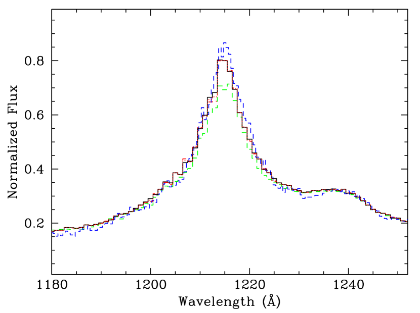
Figure 10: Ly$\alpha$ profiles of old quasars produced with different selection parameters. The black curve: the composite spectrum of current selection, as shown in the lower panel of Figure 6, which is made of median values at each wavelength bin; the green curve: with a minimum void size of 2.5 Å; the red dashed curve: with a minimum void size of 4.5 Å; and the red dotted curve: $t_{1}=1.0$. No difference is found between $t_{0}=0.2$ and 0. The blue curve is made with mean values at each pixel, using the current selection.

Figure 10 illustrates the effect on Ly$\alpha$ profiles when selection parameters vary. For a void-size limit of 2.5 Å, as shown in the green curve, the flux of Ly$\alpha$ peak is lower by approximately 10% for the composite spectrum of old quasars. When the limit is set to 4.5 Å, the red dashed curve is almost indistinguishable from that of 3.5 Å. This is because the majority of selected old quasars display void sizes greater than 5 Å. Indeed, the choice of void-size limits or the threshold levels would affect the histogram distribution in Figure 5. Higher $t_{1}$ values would lead to larger voids. As the red dotted curve in Figure 10 shows, the differences are small. If $t_{0}$ is set to zero, more voids may be identified, but it makes no difference for the subgroup of old quasars.

A test is also made to take the average flux values at each wavelength bin in the composite spectrum. As shown in the blue curve in Figure 10, the difference between the median and mean values is less than 10%. The characteristics of composite spectra of old and young quasars are therefore not just the results of a specific data analysis with certain parameters.

5 CONCLUSION

Based on the spectral voids between Ly$\alpha$ forest lines in a large sample of 2594 SDSS spectra of quasars, the proximity zones are measured to distances considerably larger than previous studies. The majority of quasars display small zones of $\lesssim 5$ Mpc in proper distance. A group of old quasars are identified with large proximity zones. They display strong narrow cores of emission lines. Another group of young quasars show infalling components ($z_{ab}>z_{em}$) and no proximity zones. The narrow Ly$\alpha$ components in these young quasars are weak. The ratio of narrow and broad components in Ly$\alpha$ increases from 0.05 for young quasars to 0.5 for old quasars.

The differences in line intensities and profiles have been a focus of quasars studies, as they are among the main PCA drivers (Boroson & Green, 1992). Suzuki (2006) carried out a PCA using 50 quasar spectra at lower redshifts and suggested four classes of different emission-line properties. Interestingly, the Class I objects in his work bear resemblance to old quasars and the Class III are similar to young quasars. The underlying reasons for such differences remain to be explored, and they could be related to quasar ages. In the early stage of a quasar’s evolution, the supermassive halo around it is rich in infalling systems. It is also possible that broad absorption lines are common at this stage. Old quasars, on the other hand, may be in an evolutionary stage that lacks infalling matter.

Ample evidence suggests that different line widths and EW are the results of viewing angles. The results presented in this paper suggest that they may also be related to quasar ages. Further studies of the broadband properties of these groups may reveal more evolution effects and shed light on the underlying reasons of known quasar properties. Since the strength of narrow cores of emission lines evolves with the sizes of proximity zones, it may serve as an age indicator at lower redshifts, when the information of forest lines is not readily available. Several known properties of emission lines, such as the Baldwin effect, may be understood in terms of quasar ages: young quasars show broad emission profiles, and narrow core become stronger in later stages as the Eddington ratio declines, and the BLR configuration changes.

Figure 1: SDSS quasars at $2.5\leq z\leq 3.5$. Only 2594 of these 3298 spectra are actually used in the analysis, as others are rejected for low quality, large redshift uncertainties, or broad absorption features.

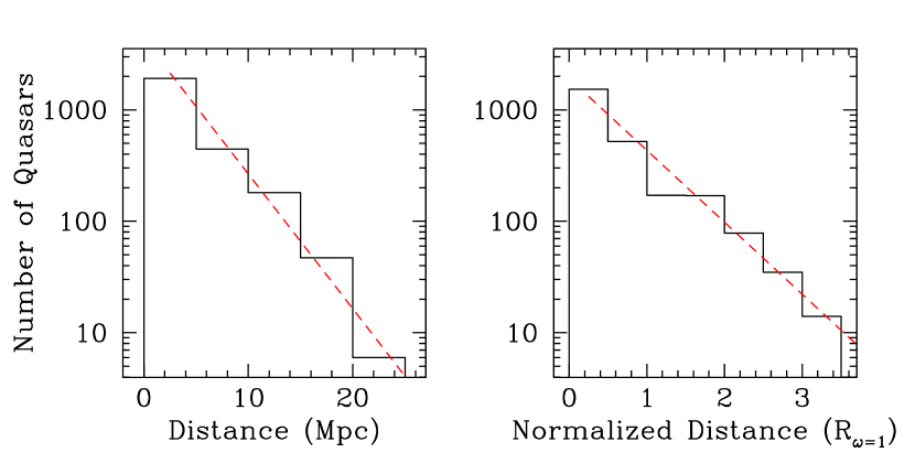
Figure 5: Distribution of proximity zones. In the right panel, proximity zones are normalized to the characteristic sizes $R_{\omega=1}$. A zone size is defined by the distance between the Ly$\alpha$ wavelength and the furthest data point in a spectral void. The samples of young and old quasars are subgroups selected with additional criteria (see §3). Both distributions can be fitted exponentially with high confidence (red lines).

Figure 6: Three composite quasar spectra with different proximity properties and implied ages. The top panel is for the young quasars with no proximity zones and with significant absorption lines longward of the Ly$\alpha$ wavelength, the middle panel for all the quasars in the sample, and the bottom panel the old quasars with large proximity zones ($>10$ Mpc). The spectra are scaled to display similar flux levels around 1350 Å.

Table 1: Equivalent Widths of Fitted Emission Lines in Composite Spectra

Line	Young		All		Old
	Broad	Narrow	Broad	Narrow	Broad	Narrow
O VI $\lambda 1035$	$12.6\pm 3.6$	$1.5\pm 0.8$	$13.4\pm 0.3$	$2.0\pm 0.1$	$17.9\pm 0.7$	$3.4\pm 0.2$
Ly$\alpha$	$50.0\pm 1.7$	$0.4\pm 1.0$	$53.9\pm 0.3$	$9.3\pm 0.2$	$51.8\pm 1.3$	$27.1\pm 0.9$
N V $\lambda 1240$	$17.0\pm 2.0$	$1.5\pm 0.4$	$10.9\pm 0.2$	$2.4\pm 0.1$	$17.2\pm 2.3$	$3.4\pm 0.2$
C IV $\lambda 1549$	$21.6\pm 1.0$	$3.5\pm 0.9$	$23.8\pm 0.3$	$5.4\pm 0.1$	$26.0\pm 0.7$	$11.3\pm 0.4$
C III] $\lambda 1909$	$18.5\pm 1.2$	$1.7\pm 0.8$	$19.8\pm 0.4$	$3.0\pm 0.3$	$18.1\pm 1.7$	$4.7\pm 0.6$
O I $\lambda 1304$	$2.1\pm 0.2$		$1.7\pm 0.1$		$2.4\pm 0.2$
C II $\lambda 1335$	$1.6\pm 0.3$		$0.7\pm 0.1$		$0.5\pm 0.1$
Si IV $\lambda 1402$	$8.9\pm 0.3$		$7.3\pm 0.2$		$6.5\pm 0.3$

Table 2: Full Widths at Half Maximum of Fitted Emission Lines in Composite Spectra

Line	Young		All		Old
	Broad	Narrow	Broad	Narrow	Broad	Narrow
Major Lines	$10915\pm 480$	$2331\pm 477$	$11155\pm 75$	$2498\pm 37$	$10002\pm 238$	$2429\pm 48$
O I $\lambda 1304$	$4080\pm 387$		$3466\pm 224$		$3362\pm 274$
C II $\lambda 1335$	$4046\pm 1093$		$2726\pm 405$		$1797\pm 521$
Si IV $\lambda 1402$	$6783\pm 239$		$5761\pm 151$		$4722\pm 223$

Table 3: Number of Spectral Voids

Void Size (Å)	Number of Voids
$\geq 3$	2217
$\geq 3.5$	1420
$\geq 4$	936
$\geq 5$	375
$\geq 6$	157
$\geq 7$	82
$\geq 8$	44
$\geq 10$	18

References

- Abazajian et al. (2009) Abazajian, K. N., Adelman-McCarthy, J. K., Agüeros, M. A., et al. 2009, ApJS, 182, 543
- Ahn et al. (2014) Ahn, C. P., Alexandroff, R., Allende Prieto, C., et al. 2014, ApJS, 211, 17
- Alam et al. (2015) Alam, S., Albareti, F. D., Allende Prieto, C., et al. 2015 ApJS, 219, 12
- Bajtlik et al. (1988) Bajtlik, S., Duncan, R. C., & Ostriker, J. P. 1988, ApJ, 327, 570
- Bechtold (1994) Bechtold, J. 1994, ApJS, 91, 1
- Blackburne et al. (2011) Blackburne, J. A., Pooley, D., Rappaport S., & Schechter, P. L. 2011, ApJ, 729, 34
- Blanton et al. (2017) Blanton, M. R., Bershady, M. A., Abolfathi, B., et al. 2017, AJ, 154, 28
- Bolton et al. (2005) Bolton, J. S., & Haehnelt, M. G., Viel, M., & Springel, V. 2005, MNRAS, 357, 1178
- Bolton & Haehnelt (2007) Bolton, J. S., & Haehnelt, M. G. 2007, MNRAS, 374, 493
- Boroson & Green (1992) Boroson, T. A., & Green, R. F. 1992, ApJS, 80, 109
- Brotherton (1996) Brotherton, M. S. 1996, ApJS, 102, 1
- Carswell et al. (1987) Carswell, R. F., Webb, J. K., Baldwin, J. A., & Atwood, B. 1987, ApJ, 319, 709
- Carswell et al. (1982) Carswell, R. F., Whelan, J. A. J., Smith, M. G., Boksenberg A., & Tytler D. 1982, MNRAS, 198, 91
- Cooke et al. (1997) Cooke, A. J., Espey, B., & Carswell, R. F. 1997, MNRAS, 284, 552
- Dall’Aglio et al. (2008a) Dall’Aglio, A., Wisotzki, L., & Worseck, G. 2008, A&A, 480, 359
- Dall’Aglio et al. (2008b) 2008, A&A, 491, 465
- DiPompeo et al. (2014) DiPompeo, M. A., Myers, A. D., Hickox, R. C., Geach, J. E., & Hainline, K. N. 2014, MNRAS, 442, 3443
- Dobrzycki & Bechtold (1991) Dobrzycki, A., & Bechtold, J. 1991, ApJL, 377, L69
- Eilers et al. (2018) Eilers, A.-C., Hennawi, J. F., & Davies, F. B. 2018, ApJ, 867, 30
- Eisenstein et al. (2011) Eisenstein, D. J., Weinberg, D. H., Agol, E., et al. 2011, AJ, 142, 72
- Elitzur (2008) Elitzur, M. 2008, New Astron. Rev., 52, 274
- Elvis et al. (1994) Elvis, M., Wilkes, B. J., McDowell, J. C., et al. 1994, ApJS, 95, 1
- Fine et al. (2011) Fine, S., Jarvis, M. J., & Mauch, T. 2011, MNRAS, 412, 213
- Friedman et al. (2008) Frieman, J. A., Bassett, B., Becker, A., et al. 2008, AJ, 135, 338
- Giallongo et al. (1996) Giallongo, E., Christiani, S., DÓdorico, S., Fontana, A., & Savaglio, S. 1996, ApJ, 466, 46
- Guimarães et al. (2007) Guimarães, R., Petitjean, P., Rollinde, E., et al. 2007, MNRAS, 377, 657
- Hewett & Wild (2010) Hewett, P. C., & Wild, V. 2010, MNRAS, 405, 2302
- Hu et al. (2008) Hu, C., Wang, J.-M., Ho, L., et al. 2008, ApJ, 683, L115
- Jakobsen et al. (2003) Jakobsen, P., Jansen, R. A., Wagner, S., & Reimers, D. 2003, A&A, 397, 891
- Janknecht et al. (2006) Janknecht, E., Reimers, D., Lopez, S., & Tytler, D. 2006, A&A, 458, 427
- Kauffmann & Haehnelt (2000) Kauffman, G., & Haehnelt, M. 2000, MNRAS, 311, 576
- Khrykin et al. (2016) Khrykin, I. S., Hennawi, J. F., McQuinn, M., & Worseck, G. 2016, ApJ, 824, 133
- Khrykin et al. (2019) Khrykin, I. S., Hennawi, J. F., & Worseck, G. 2019, MNRAS, 484, 3897
- Kirkman & Tytler (2008) Kirkman, D., & Tytler, D. 2008, MNRAS, 391, 1457
- Kriss (1994) Kriss, G. A. 1994, in Astronomical Data Analysis Software, and Systems III, eds. D. R. Crabtree, R. J. Hanisch, & J. Barnes, (A. S. P. Conf. Series 61, ASP, San Francisco), 437
- Lau et al. (2016) Lau, M. W., Prochaska, J. X., & Hennawi, J. F. 2016, ApJS, 226, 25
- Liske & Williger (2001) Liske, J., & Williger, G. M. 2001, MNRAS, 328, 653
- Lu et al. (1996) Lu, L., Sargent, W. L. W., Womble, D. S., & Takada-Hidai, M. 1996, ApJ, 472, 509
- Lu & Yu (2011) Lu, Y., & Yu, Q. 2011, ApJ, 736, 49
- Martini (2004) Martini, P., 2004, in Coevolution of Black Holes and Galaxies, ed. L. C. Ho, (Cambridge University Press, Cambridge, U. K.), 169
- McQuinn (2016) McQuinn, M. 2016, ARAA, 54, 313
- Meiksin (2006) Meiksin, A. 2006, MNRAS, 365, 807
- Meiksin (2009) 2009, RevMP, 841, 1405
- Meiksin & McQuinn (2019) Meiksin, A., & McQuinn, M. 2019, MNRAS, 482, 4777
- Murdoch et al. (1986) Murdoch, H. S., Hunstead, R. W., Pettini, M., & Blades, J. C. 1986, ApJ, 309, 19
- Pâris et al. (2014) Pâris, I., Petitjean, P., Aubourg, É, et al. 2014, A&A, 563, 54
- Pâris et al. (2018) 2018, A&A, 613, A51
- Pâris et al. (2017) Pâris, I., Petitjean, P., Ross, N., et al. 2017, A&A, 597, A79
- Rudge & Raine (1997) Rudge, C. M., & Raine, D. J. 1997, MNRAS, 297, L1
- Schmidt et al. (2018) Schmidt, T. M., Hennawi, J. F., Worseck, G., et al. 2018, ApJ, 861, 122
- Schmidt et al. (2017) Schmidt, T. M., Worseck, G., Hennawi, J. F., et al. 2017, ApJ, 847, 81
- Schneider et al. (2010) Schneider, D. P., Richards, G. T., Hall, P. B., et al. 2010, AJ, 139, 2360
- Scott et al. (2000) Scott, J., Bechtold, J., Dobrzycki, A., & Kulkarni, V. P. 2000, ApJS, 130, 67
- Shang et al. (2011) Shang, Z., Brotherton, M. S., Wills, B. J. et al. 2011, ApJS, 196, 2
- Shull et al. (2010) Shull, J. M., France, K., Danforth, C. W., & Smith, B. 2010, ApJ, 722, 1312
- Simpson (2005) Simpson, C. 2005, MNRAS, 360, 565
- Springel et al. (2005) Springel, V., White, S. D. M., Jenkins, A., et al. 2005, Nature, 435, 629
- Suzuki (2006) Suzuzi, N. 2006, ApJS, 163, 110
- Syphers & Shull (2014) Syphers, D., & Shull, J. M. 2014, ApJ, 784, 42
- Telfer et al. (2002) Telfer, R., Zheng, W., Kriss, G. A., & Davidsen, A. F. 2002, ApJ, 565, 733
- Tytler (1987) Tytler, D. 1987, ApJ, 321, 49
- Urry & Padovani (1995) Urry, C. M., & Padovani, P. 1995, PASP, 107, 803
- White et al. (2003) White, R. L., Becker, R., Fan, X., & Strauss, M. A. 2003, AJ, 126, 1
- York et al. (2000) York, D. G., Adelman, J., Anderson, J. E. Jr., et al. 2000, AJ, 120, 1579
- Yuan et al. (2016) Yuan, S., Strauss, M. A., & Zakamska, N. L. 2016, MNRAS, 462, 1603
- Zakamska et al. (2003) Zakamska, N. L., Strauss, M. A., Krolik, J. H., et al. 2003, AJ, 126, 2125
- Zheng & Davidsen (1995) Zheng, W., & Davidsen, A. F. 1995, ApJL, 440, L53
- Zheng et al. (1997) Zheng, W., Kriss, G. A., Telfer, R. C., Grimes, J. P., & Davidsen, A. D. 1997, ApJ, 475, 469
- Zheng et al. (2019) Zheng, W., Meiksin, A., & Syphers, D. 2019, ApJ, 883, 123
- Zheng et al. (2015) Zheng, W., Syphers, D., Meiksin, A., et al. 2015, ApJ, 806, 142
- Zhu et al. (2009) Zhu, L., Zhang, S. N., & Tang, S., 2009, ApJ, 700, 1173