The Maximum-Level Vertex in an Arrangement of Lines

Abstract

Let $L$ be a set of $n$ lines in the plane, not necessarily in general position. We present an efficient algorithm for finding all the vertices of the arrangement ${\cal A}(L)$ of maximum level, where the level of a vertex $v$ is the number of lines of $L$ that pass strictly below $v$. The problem, posed in Exercise 8.13 in de Berg et al. [dBCKO08], appears to be much harder than it seems, as this vertex might not be on the upper envelope of the lines.

We first assume that all the lines of $L$ are distinct, and distinguish between two cases, depending on whether or not the upper envelope of $L$ contains a bounded edge. In the former case, we show that the number of lines of $L$ that pass above any maximum level vertex $v_{0}$ is only $O(\log n)$. In the latter case, we establish a similar property that holds after we remove some of the lines that are incident to the single vertex of the upper envelope. We present algorithms that run, in both cases, in optimal $O(n\log n)$ time.

We then consider the case where the lines of $L$ are not necessarily distinct. This setup is more challenging, and the best we have is an algorithm that computes all the maximum-level vertices in time $O(n^{4/3}\log^{3}n)$.

Finally, we consider a related combinatorial question for degenerate arrangements, where many lines may intersect in a single point, but all the lines are distinct: We bound the complexity of the weighted $k$-level in such an arrangement, where the weight of a vertex is the number of lines that pass through the vertex. We show that the bound in this case is $O(n^{4/3})$, which matches the corresponding bound for non-degenerate arrangements, and we use this bound in the analysis of one of our algorithms.

1 Introduction

Let $L$ be a set of $n$ lines in the plane, not necessarily in general position (that is, there may be points incident to more than two lines of $L$, and pairs of lines of $L$ might be parallel or even coincide). The largest part of the paper is devoted to the case where the lines of $L$ are pairwise distinct; the more difficult case where lines of $L$ might coincide will be handled later on. We wish to find a vertex, or rather all the vertices, of the arrangement ${\cal A}(L)$ at maximum level, where the level $\lambda(v)$ of a vertex $v$ is the number of lines of $L$ that pass strictly below $v$.

The question that we address here appears as an exercise in the computational geometry textbook by de Berg et al. [dBCKO08, Exercise 8.13]. It can be solved in quadratic time by constructing the full arrangement, and then by tracing the vertices along each line from left to right, keeping track of the level of each vertex as we go. The challenge is of course to solve it faster.

If we assume general position (so no three lines pass through a common point), then every vertex on the upper envelope of $L$ is at level $n-2$, which is the maximum possible level (and only the vertices of the envelope have this level). Finding one such vertex in linear time is straightforward, and finding all of them takes $O(n\log n)$ time. Henceforth we focus on the interesting, and harder, case where the lines are not in general position. For this setting we are not aware of any previous subquadratic-time algorithm to compute a maximum-level vertex. As the requirement of Exercise 8.13 in [dBCKO08] was to solve the problem in $O(n\log n)$ time, it seems that the difficulty of the problem was overlooked there.

The main obstacle is that, in degenerate situations, the desired vertex does not have to lie on the upper envelope of $L$, as shown in the example depicted in Figure 1.2.

Figure 1.1: A set $L$ of lines for which the vertex of ${\cal A}(L)$ of maximum level, which is $v_{0}$, does not lie on the upper envelope.	Figure 1.2: A more “substantial” construction, in which the horizontal line $\ell$ contains all but one of the vertices of ${\cal A}(L)$, all at upper level $\Theta(n)$. The maximum-level vertex is $v_{0}$ (as well as its symmetric counterpart on the other side of $\ell$).

In fact, the situation can be much worse—the vertex at maximum level can be far away from the upper envelope. An illustration of such a case is given in Figure 1.2.

We do not solve exercise 8.13 completely. We give an $O(n\log n)$ algorithm only for the case of distinct lines. For the case where the lines in $L$ are not necessarily distinct we only give an $O(n^{4/3}\log^{3}n)$ algorithm. In either case, we may assume that $L$ does not contain any vertical line: any such line is not counted in the level of any point, and the only role of such lines is to create new vertices of the arrangement. For any vertical line $\ell$, the only relevant vertex is the highest intersection point of $\ell$ with other lines of $L$. It is straightforward to find, in $O(n\log n)$ overall time, these highest intersection points and their levels, for all vertical lines. Therefore, in what follows, we can indeed assume that $L$ has no vertical lines.

Consider in what follows the case where all the lines of $L$ are distinct; as already noted, the case of coinciding lines is subtler and is discussed in detail in Section 4.

Similar to the case of vertices, a point $p$ in the plane is said to be at level $k$, if there are exactly $k$ lines in $L$ passing strictly below $p$. The level of a (relatively open) edge $e$ (resp., face $f$) of ${\cal A}(L)$ is the level of any point of $e$ (resp., $f$). The $k$-level of ${\cal A}(L)$ is the closure of the union of the edges of ${\cal A}(L)$ that are at level $k$. The at-most-$k$-level of ${\cal A}(L)$, or $(\leq k)$-level, is the closure of the union of the edges of ${\cal A}(L)$ at levels $j$, $0\leq j\leq k$. We denote the $k$-level as $\Lambda^{\downarrow}_{k}$, and the at-most-$k$-level as $\Lambda^{\downarrow}_{\leq k}$.

In complete analogy, we define the upper level of a vertex $v$ in ${\cal A}(L)$ (or of any point $v\in\mathbb{R}^{2}$) to be the number of lines of $L$ that pass strictly above $v$. The $k$-upper level and the $({\leq}k)$-upper level of ${\cal A}(L)$ are defined analogously to the standard level, and are denoted as $\Lambda^{\uparrow}_{k}$ and $\Lambda^{\uparrow}_{\leq k}$, respectively.

We consider two complementary cases:

Case (i): The upper envelope of $L$ contains a bounded edge, and thus has at least two vertices; see Figure 1.2.

Case (ii): The upper envelope of $L$ does not contain a bounded edge, and thus consists of a single vertex and two rays; see Figure 1.2.

The main combinatorial results that provide the basis for our algorithms are summarized in the following two theorems.

Theorem 1.1.

Let $L$ be a set of $n$ distinct lines in the plane that satisfies the assumption of Case (i). Then the upper level of any maximum-level vertex of ${\cal A}(L)$ is at most $2\log n$.

For Case (ii) we can achieve a similar property with some additional preparation. Specifically, let $v$ be the single vertex of the upper envelope of $L$, let $L_{v}$ denote the set of the lines of $L$ that are incident to $v$, and set $K:=L\setminus L_{v}$. Assume that $K$ is nonempty; if $K=\emptyset$ then $v$ is the only vertex of ${\cal A}(L)$, which is clearly of maximum level (which is $0$). For each line $\ell\in L_{v}$, let $\ell^{-}$ (resp., $\ell^{+}$) denote the portion (ray) of $\ell$ to the left (resp., right) of $v$. Set $L_{v}^{-}=\{\ell^{-}\mid\ell\in L_{v}\}$ and $L_{v}^{+}=\{\ell^{+}\mid\ell\in L_{v}\}$. Sort the rays of $L_{v}^{-}$ downwards, i.e., in increasing order of their slopes, and sort the rays of $L_{v}^{+}$ also downwards, now in decreasing order of their slopes. Let $D^{-}$ (resp., $D^{+}$) denote the size of the largest prefix of the rays of $L_{v}^{-}$ (resp., $L_{v}^{+}$) that do not intersect any line of $K$ (and thus any other line of $L$), and put $D:=\min\{D^{-},D^{+}\}$. See Figure 1.3.

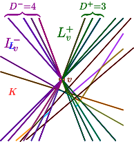
Figure 1.3: The case of a single vertex on the upper envelope. The same arrangement is depicted three times, with different notations.

Since $K\neq\emptyset$, it easily follows that no line $\ell$ of $L_{v}$ can contribute rays to both prefixes of $L_{v}^{-}$ and $L_{v}^{+}$ defined above (unless all lines of $K$ are parallel to $\ell$, an easily handled situation that we ignore here).

Put $h:=\max\{0,D-2\log n\}$ and $D_{0}:=D-h=\min\{D,2\log n\}$. Remove from $L$ the lines that contribute the $h$ topmost rays to $L_{v}^{-}$ and the lines that contribute the $h$ topmost rays to $L_{v}^{+}$; by what has just been said, no line is removed twice, and we are thus left with a subset $L_{0}$ of $L$ of size $n-2h$.

Theorem 1.2.

Let $L$ be a set of $n$ distinct lines in the plane that satisfies the assumption of Case (ii). Let $v$, $L_{v}$, $K$, $D$, $h$, $D_{0}$ and $L_{0}$ be as defined above. Then all the maximum-level vertices of ${\cal A}(L)$ are vertices of ${\cal A}(L_{0})$, and the upper level in ${\cal A}(L_{0})$ of any maximum-level vertex of ${\cal A}(L)$ is at most $4\log n$.

We will exploit these theorems in designing efficient algorithms, that run in optimal $O(n\log n)$ time, for computing all the maximum-level vertices, in both cases. We note that this running time is indeed optimal: Even the task of computing the upper envelope of $L$ is at least as hard as the task of sorting the lines by slope.

A central ingredient of our algorithms is computing the at-most-$k$-upper level of an arrangement, where $k=O(\log n)$. The complexity (number of edges and vertices) of the $({\leq}k)$-level in an arrangement of $n$ lines is $\Theta(nk)$ [AG86, CS89]. Typically, this is shown for arrangements of lines in general position, by an easy application of the Clarkson-Shor random sampling theory [CS89], but it also holds in degenerate situations, as can easily be verified. The $({\leq}k)$-level can be computed, for arrangements in general position, in optimal time $O(n\log n+nk)$ by an algorithm of Everett et al. [ERK96]. We sketch (our interpretation of) the algorithm in Appendix A. As $k=O(\log n)$ in both cases, the algorithm runs in (optimal) $O(n\log n)$ time. It is not clear, though, whether this (fairly involved) algorithm also works for degenerate arrangements.

To finesse this issue, we run the algorithm of [ERK96] on perturbed copies of the lines of $L$, using a simplified variant of symbolic perturbation, and then extract from its output the actual at-most-$k$-level in the original degenerate arrangement. In a fully symmetric manner, this construction also applies to the at-most-$k$-upper levels of ${\cal A}(L)$.

We remark that levels can be defined for arrangements of objects other than lines and in higher dimensions. Levels in arrangements of hyperplanes are closely related (by duality) to so-called $k$-sets in configurations of points. Both structures have been extensively studied; see the recent survey on arrangements [HS18] for a review of bounds and algorithms. In what follows, though, we only concern ourselves with planar arrangements of lines.

The paper is organized as follows. In Section 2 we give the proofs of Theorem 1.1 and Theorem 1.2, and then present, in Section 3, our efficient (optimal) algorithms for both cases. The case where $L$ can contain coinciding lines is discussed in Section 4, where we present an algorithm that has a weaker $O(n^{4/3}\log^{3}n)$ upper bound on its complexity. We conclude in Section 5 with a bound on the maximum complexity of the weighted $k$-level in arrangements of lines, still catering to the case where many lines may intersect in a single point, but the lines are all distinct. Here the weight of a vertex is the number of lines that pass through it, and the complexity of the weighted level is the sum of the weights of its vertices. On top of being a result of independent interest, we exploit it in the analysis of our algorithm for the case of coinciding lines. In the Appendix we give a brief review of the optimal-time algorithm by Everett et al. [ERK96] for computing the $({\leq}k)$-level for arrangements of lines in general position, describing it from a different (and, to us, simpler) perspective than the original paper.

2 The upper level of maximum-level vertices

The proofs of both Theorem 1.1 and Theorem 1.2 rely on the following structural property, which we regard as interesting in its own right.

Consider the $k$-upper level $\Lambda^{\uparrow}_{k}$, which, as we recall, is the $x$-monotone polygonal curve which is the closure of the union of the edges of the arrangement with exactly $k$ lines above each of them. Since the lines of $L$ are distinct, these levels do not share any edge, but they can share vertices. The degree of a vertex is the number of lines in $L$ incident to the vertex. A vertex of degree $d$ appears in $d$ consecutive levels. Note that the level does not necessarily turn at every vertex $v$ that it reaches: it could pass through $v$ staying on the same line (this happens when the degree of $v$ is odd and the level reaches $v$ along the median incident line). See Figure 2.1 for an illustration.

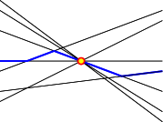
Figure 2.1: The highlighted level does not turn at the marked vertex.

Let $k_{0}$ be the smallest index such that there exists some vertex $v$ that lies strictly above $\Lambda^{\uparrow}_{k_{0}}$ (so $v$ is a vertex of $\Lambda^{\uparrow}_{k_{0}-1}$, but not necessarily of all the preceding upper levels). The vertices lying strictly above $\Lambda^{\uparrow}_{k_{0}}$ are called detached. See Figure 2.2.

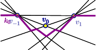
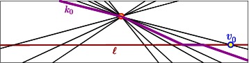
Figure 2.2: Figure 1.2 and a variant of Figure 1.2 with the $k_{0}$-upper level highlighted.

Lemma 2.1.

A vertex has maximum level if and only if it lies above $\Lambda^{\uparrow}_{k_{0}}$. The maximum level is $n-k_{0}$.

Proof. Let $v$ be any detached vertex. We claim that the level $\lambda(v)$ of $v$ is exactly $n-k_{0}$. This is because there are exactly $k_{0}$ lines that pass through or above $v$, which follows since (i) this is the number of lines that cross the vertical line through $v$ above $\Lambda^{\uparrow}_{k_{0}}$, and (ii) none of these lines passes between $v$ and $\Lambda^{\uparrow}_{k_{0}}$, by definition.

Except for potential other vertices that lie, like $v$, strictly above $\Lambda^{\uparrow}_{k_{0}}$, and whose level is thus also $n-{k_{0}}$, any other vertex $w$ lies on or below $\Lambda^{\uparrow}_{k_{0}}$. Suppose that $w$ lies on $\Lambda^{\uparrow}_{k_{0}}$. Move from $w$ slightly to its left, say, along an adjacent edge of $\Lambda^{\uparrow}_{k_{0}}$. The new point $w^{\prime}$ has exactly ${k_{0}}$ lines above it and exactly one line through it, so its level satisfies $\lambda(w^{\prime})=n-{k_{0}}-1$. This implies that $\lambda(w)$ is at most $n-{k_{0}}-1$, as we clearly must have $\lambda(w)\leq\lambda(w^{\prime})$; see Figure 2.3. The case where $w$ lies on an upper level of a larger index is handled similarly, and in fact its level can only get smaller. This completes the proof. $\Box$

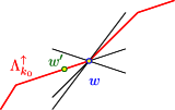
Figure 2.3: The level of any vertex $w$ of $\Lambda^{\uparrow}_{k_{0}}$ is at most $n-k_{0}-1$.

To exploit this result, we need the following property.

Lemma 2.2.

Assume that, for some $k\geq 0$, $\Lambda^{\uparrow}_{k}$ has at least two vertices, and that all the vertices of $\Lambda^{\uparrow}_{k}$ also belong to $\Lambda^{\uparrow}_{k+1}$. Then, denoting by $V_{j}$ the number of vertices of $\Lambda^{\uparrow}_{j}$, for any $j$, we have $V_{k+1}\geq 2V_{k}-1$.

Proof. The claim follows trivially by observing that if $a$ and $b$ are two consecutive vertices of $\Lambda^{\uparrow}_{k}$, and thus also of $\Lambda^{\uparrow}_{k+1}$, then $\Lambda^{\uparrow}_{k+1}$ must contain at least one additional vertex between $a$ and $b$. See Figure 2.4. Indeed, $\Lambda^{\uparrow}_{k+1}$ leaves $a$ (to the right) on a different edge than $ab$. Similarly, $\Lambda^{\uparrow}_{k+1}$ enters $b$ (from the left) on a different edge than $ab$. These two edges must be distinct, which implies that there must be at least one vertex in between them on $\Lambda^{\uparrow}_{k+1}$. $\Box$

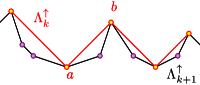
Figure 2.4: Proof of Lemma 2.2. Any pair of consecutive upper levels $\Lambda^{\uparrow}_{k},\Lambda^{\uparrow}_{k+1}$, such that all the vertices of $\Lambda^{\uparrow}_{k}$ are also vertices of $\Lambda^{\uparrow}_{k+1}$, have the property that $V_{k+1}\geq 2V_{k}-1$.

Note that the lemma also holds trivially when $V_{k}=1$, except that then it only implies the trivial inequality $V_{k+1}\geq 1$.

2.1 Upper Bounds

We now complete the proofs of both Theorem 1.1 and Theorem 1.2.

Proof of Theorem 1.1 (Case (i)).

By assumption, in this case $\Lambda^{\uparrow}_{0}$ has at least two vertices. Hence, $V_{0}\geq 2$, and Lemma 2.2 implies that $V_{1}\geq 3$, and in general $V_{k}\geq 2^{k}+1$, as is easily verified, for every $k\leq k_{0}-1$, where $k_{0}$ is the index introduced prior to Lemma 2.1. Hence, since the number of (distinct) vertices of ${\cal A}(L)$ is at most $\binom{n}{2}$, it follows that after at most $2\log n-1$ upper levels, the assumption of Lemma 2.2 can no longer hold, and, at the next upper level, which we have denoted as $k_{0}$, we get at least one vertex of $\Lambda^{\uparrow}_{k_{0}-1}$ that lies strictly above $\Lambda^{\uparrow}_{k_{0}}$, and, by Lemma 2.1, any such vertex has maximum level (and only these vertices have this property). This completes the proof of Theorem 1.1. $\Box$

Proof of Theorem 1.2 (Case (ii)).

This case is slightly more involved. Let $v$, $L_{v}$, $K$, $D$, $h$, $D_{0}$ and $L_{0}$ be as defined prior to the theorem statement. In this case, each of the first $D$ upper levels $\Lambda^{\uparrow}_{0}$, $\Lambda^{\uparrow}_{1}$, …, $\Lambda^{\uparrow}_{D-1}$ will have just a single vertex, namely $v$, but $\Lambda^{\uparrow}_{D}$ has at least one new vertex that is an intersection of some line of $K$ with either the $(D+1)$-st highest left ray or the $(D+1)$-st highest right ray emanating from $v$ (rays are numbered starting at 1).

From this level on, Lemma 2.2 can be applied, and it implies that there exists a level among the subsequent levels $\Lambda^{\uparrow}_{D}$, $\Lambda^{\uparrow}_{D+1}$, …, $\Lambda^{\uparrow}_{D+2\log n}$ of ${\cal A}(L)$, for which there exists a vertex that lies strictly above the level, and, at the first time this happens, any such detached vertex has maximum level in ${\cal A}(L)$, by Lemma 2.1 (and only these vertices have this property). If $D\leq 2\log n$ then no line is removed, and both claims of the theorem (that all the maximum-level vertices of ${\cal A}(L)$ are vertices of ${\cal A}(L_{0})$, and that the upper level in ${\cal A}(L_{0})$ of the maximum-level vertices is at most $4\log n$) hold; the first is trivial and the second follows from $D+2\log n\leq 4\log n$. Assume then that $D>2\log n$. In this case $D_{0}=2\log n$. Since no line $\ell\in L_{v}$ contributes to both prefixes of $L_{v}^{-}$ and $L_{v}^{+}$ of length $D$, at least $2D$ upper levels of ${\cal A}(L)$ pass through $v$. In particular, $v$ lies on all levels $\Lambda^{\uparrow}_{0}$ to $\Lambda^{\uparrow}_{D+2\log n}$. We claim that none of the $2h$ lines removed from $L$ can meet any of the upper levels $\Lambda^{\uparrow}_{h}=\Lambda^{\uparrow}_{D-2\log n}$ to $\Lambda^{\uparrow}_{D+2\log n}$ of ${\cal A}(L)$, except for passing through it at $v$. Indeed, any line $\ell$ that contributes a ray to the top $h$ rays of $L_{v}^{+}$ passes to the right of $v$ above at least $D_{0}=2\log n$ other lines of $L_{v}$, none of which has been removed, so $\ell$ passes below all these lines to the left of $v$ and thus cannot meet the topmost $D+2\log n$ levels of ${\cal A}(L)$ to the left of $v$, and it clearly cannot do so to the right of $v$. Figure 2.5 illustrates this argument. The argument for lines that contribute a ray to the top $h$ rays of $L_{v}^{-}$ is fully symmetric. We conclude that upper levels $\Lambda^{\uparrow}_{h}=\Lambda^{\uparrow}_{D-2\log n}$ to $\Lambda^{\uparrow}_{D+2\log n}$ of ${\cal A}(L)$ are identical to levels $\Lambda^{\uparrow}_{0}$ to $\Lambda^{\uparrow}_{4\log n}$ of ${\cal A}(L_{0})$, and hence the upper level of any point in these levels (except for $v$) with respect to $L$ is $h$ plus its upper level with respect to $L_{0}$. Thus their upper level with respect to $L_{0}$ is at most $D+2\log n-h=4\log n$. All this completes the proof of the theorem. $\Box$

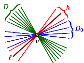
Figure 2.5: The prefixes of length $D$ of $L_{v}^{-}$ and $L_{v}^{+}$ are indicated in green and red/blue respectively. No line of $L_{v}$ contributes to both prefixes. To the left of $v$ any of the $h$ red lines has at least $D+D_{0}=D+2\log n$ lines above it.

2.2 Lower Bound

In this subsection we give a construction that satisfies the property of Case (i), for which the upper level of all the maximum-level vertices is $\Omega(\log n)$. We put $m=2^{t}$, for some integer $t$, and construct the set $P$ of the $2m+1$ points $p_{-m},\ldots,p_{-1},p_{0},p_{1},\ldots,p_{m}$ on the parabola $\gamma:\;y=x^{2}$, where

$$p_{0} =(0,0),$$

$$p_{i} =(3^{i-1},3^{2(i-1)}),\qquad\text{for $i=1,\ldots,m$}$$

$$p_{-i} =(-3^{i-1},3^{2(i-1)}),\qquad\text{for $i=1,\ldots,m$}.$$

For each $j=0,\ldots,t$, we construct a set $L_{j}$ of $s_{j}=2^{j+1}$ ‘dyadic’ lines. Concretely, for each $j$ we set $L_{j}=L_{j}^{-}\cup L_{j}^{+}$, where the $r$th line in $L_{j}^{+}$ connects the points $p_{(r-1)2^{t-j}}$ and $p_{r2^{t-j}}$, for $r=1,\ldots,2^{j}$, and the lines of $L_{j}^{-}$ are reflected copies of the lines of $L_{j}^{+}$ about the $y$-axis (so the $r$th line in $L_{j}^{-}$ connects the points $p_{-(r-1)2^{t-j}}$ and $p_{-r2^{t-j}}$, for $r=1,\ldots,2^{j}$). We put $L:=\bigcup_{j=0}^{t=1}L_{j}$, and note that $|L|=\sum_{j=0}^{t}2^{j+1}=2^{t+2}-2$. See Figure 2.6 for an illustration.

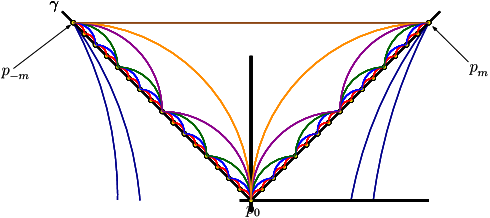
Figure 2.6: A schematic illustration of the construction, where the parabola is flattened to a V shape and the scale is logarithmic.

Lemma 2.3.

(a) All the intersection points of the lines of $L$ are either points of $P$ or lie below the parabola $\gamma$.
(b) All these intersection points lie in the $x$-range between $p_{-m}$ and $p_{m}$.

Proof. Associate with each line $\ell\in L$ the arc $\gamma_{\ell}$ of $\gamma$ between the two points of $P$ that $\ell$ connects. By construction, each pair of these arcs are either openly disjoint or nested within one another. This immediately implies (a). For (b), consider a pair of lines $\ell,\ell^{\prime}\in L$. The claim trivially holds when $\gamma_{\ell}$ and $\gamma_{\ell^{\prime}}$ are openly disjoint, as the intersection point lies in the $x$-range between the two arcs. Assume then that the arcs are nested, say $\ell$ connects $p_{u}$ and $p_{v}$, $\ell^{\prime}$ connects $p_{w}$ and $p_{z}$, and $u\leq w<z\leq v$. If $u=w$ or $z=v$, the lines intersect at a point of $P$ and the claim follows, so assume that $u<w<z<v$. The construction allows us to assume, without loss of generality, that $0\leq u<w<z<v$. Assume first that $u>0$. To simplify the notation, write $a=3^{u-1}$, $b=3^{v-1}$, $c=3^{w-1}$, and $d=3^{z-1}$. Let the intersection point be $(x,y)$. Then we have

$$\frac{y-a^{2}}{b^{2}-a^{2}} =\frac{x-a}{b-a}, (a,a^{2}),(b,b^{2}) (x,y)$$ for the line passing through and

$$\frac{y-c^{2}}{d^{2}-c^{2}} =\frac{x-c}{d-c}, \text{for the line passing through $(c,c^{2}),(d,d^{2})$ and $(x,y)$}\;,$$

and it thus follows that

$$x=\frac{ab-cd}{a+b-c-d}.$$

We claim that $-b<x<b$, from which (b) follows. Observing that $b>3c$ and $b>3d$, the denominator is positive, so we need to show that

$$-b(a+b-c-d)<ab-cd<b(a+b-c-d).$$

Divide everything by $a^{2}$, and put $C=c/a$, $D=d/a$, and $B=b/a$. We thus need to show that

$$-B(1+B-C-D)<B-CD<B(1+B-C-D).$$

The right inequality becomes $(B-C)(B-D)>0$, which clearly holds as $B>C,D$. The left inequality becomes $B^{2}+2B>CD+BC+BD$, which also holds since $C,D\leq B/3$.

The case $u=0$ is handled in exactly the same manner, except that we replace $a$ by $0$. It is easily checked that the required inequalities continue to hold. This completes the proof. $\Box$

To complete the construction, we generate two additional arbitrary lines that pass through $p_{m}$ and are contained in the acute-angled cone spanned by the tangent to $\gamma$ at $p_{m}$ and the vertical line through $p_{m}$, and apply the same construction at $p_{-m}$. Altogether we obtain a set $L^{\prime}$ of $n=2^{t+2}+2$ lines. It is easily checked that any intersection point formed by any of the new lines also lies in the $x$-range between $p_{-m}$ and $p_{m}$. This, combined with Lemma 2.3, imply that the upper level of any vertex of ${\cal A}(L^{\prime})$ that lies below $\gamma$ is at least $t+1$, implying that the actual level of any such vertex is at most $n-t-3$. It thus remains to calculate the levels of the points of $P$.

For $p_{m}$, we have $t+3$ lines passing through this point, and no line of $L^{\prime}$ passes above it, so its level is $n-t-3$. The same holds for $p_{-m}$. For any other $p_{u}$, with $u\neq 0$, let $j$ be the largest integer such that $2^{j}$ divides $u$; for $u=0$ set $j=t$. Then, by construction, there is exactly one line of $L_{i}$, for each $i<t-j$, that passes above $p_{u}$, and two lines of $L_{i}$ are incident to $p_{u}$, for each $i\geq t-j$. Hence the number of lines that pass through or above $p_{u}$ is (exactly)

$$2(j+1)+(t-j)=t+j+2,$$

implying that the level of $p_{u}$ is $n-t-j-2$. The maximum value is attained for $j=0$, which is $n-t-2$. This is therefore the maximum level of a vertex of ${\cal A}(L)$, and all the vertices with $j=0$ (those with odd indices) have $t-1=\Theta(\log n)$ lines of $L$ passing above them; that is, their upper level is $\Theta(\log n)$.

3 Algorithms

We now present an efficient, $O(n\log n)$-time algorithm for each of the two cases.

Case (i).

Here we need to construct the $k:=2\log n$ upper levels of ${\cal A}(L)$ and report any detached vertex (or, for that matter, all detached vertices) of maximum level. We use the algorithm of Everett et al. [ERK96], but we want to run it on a set of lines in general position. For this, we perturb each line $\ell_{1},\ldots,\ell_{n}$ of $L$, using a special kind of symbolic perturbation that uses only parallel shifts. That is, each line $\ell_{i}$, with equation $y=a_{i}x+b_{i}$, is replaced by a line $\ell^{\prime}_{i}$, given by $y=a_{i}x+b_{i}+{\varepsilon}_{i}$, where the ${\varepsilon}_{i}$’s are symbolic infinitesimal values, satisfying ${\varepsilon}_{1}\gg{\varepsilon}_{2}\gg\cdots\gg{\varepsilon}_{n}$. Let $L^{\prime}$ denote the set of perturbed (actually, shifted) lines. We apply the algorithm of [ERK96] to $L^{\prime}$, to compute the $k$ upper levels of ${\cal A}(L^{\prime})$, in time $O(nk+n\log n)=O(n\log n)$.

We resolve any comparison that the algorithm performs using the varying orders of magnitude of the ${\varepsilon}_{i}$’s. As a concrete illustration, consider a comparison between (the $x$-coordinates of) two intersection points of some line $\ell_{i}$ with two other lines $\ell_{j}$, $\ell_{m}$. (We may assume that $\ell_{i}$ is parallel to neither $\ell_{j}$ nor to $\ell_{m}$.) The $x$-coordinates of the two intersection points are

$$x_{i,j}=-\frac{b_{j}-b_{i}}{a_{j}-a_{i}}-\frac{{\varepsilon}_{j}-{\varepsilon}_{i}}{a_{j}-a_{i}},\qquad\text{and}\qquad x_{i,m}=-\frac{b_{m}-b_{i}}{a_{m}-a_{i}}-\frac{{\varepsilon}_{m}-{\varepsilon}_{i}}{a_{m}-a_{i}}.$$

When comparing these values, if the non-infinitesimal terms in these expressions are unequal, the outcome of the comparison is straightforward. If they are equal, the difference between these $x$-coordinates is a linear combination of ${\varepsilon}_{i}$, ${\varepsilon}_{j}$, and ${\varepsilon}_{m}$. Using the different orders of magnitude of these parameters, we can easily obtain the sign of the comparison.

Similar actions can be taken for any of the other basic operations that the algorithm performs. Clearly, the cost of each basic operation, including the cost of resolving comparisons via the symbolic perturbation technique, is still constant.

It is straightforward to extract from the output of the algorithm the top $k$ levels as a collection of edge-disjoint $x$-monotone polygonal curves.

Transforming each perturbed level into the corresponding level in the original arrangement.

Fix some index $j\leq k$. We delete all the infinitesimal edges in $\Lambda^{\uparrow}_{j}$ of $\mathcal{A}(L^{\prime})$ to obtain a left-to-right sequence $s_{1},s_{2},\ldots,s_{q}$, where $s_{1}$ and $s_{q}$ are rays and the remaining $s_{i}$’s are bounded segments. The $x$-projections of these elements are pairwise openly disjoint, and they might have (infinitesimal) gaps between them (due to the deletion of in-between infinitesimal edges). We define the function $F$ so that it associates with each segment $s_{i}$, which is supported by some (unique) perturbed line $\hat{\ell}_{m}$, the unperturbed $\ell_{m}$, namely $F(s_{i})=\ell_{m}$. With each pair of consecutive segments $s_{i},s_{i+1}$, we associate the intersection point of their associated lines $F(s_{i})\cap F(s_{i+1})$, unless $F(s_{i})=F(s_{i+1})$. In the latter case, the level progresses from $s_{i}$ to $s_{i+1}$ along the same line $F(s_{i})=F(s_{i+1})$ of $L$, and we therefore merge the segments $s_{i}$ and $s_{i+1}$ into a single segment, ignore the activity in the perturbed level near the infinitesimally-separated endpoints of $s_{1}$ and $s_{2}$, and proceed to handle the next pair $s_{i+1},s_{i+2}$. See Figure 3.1.

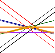
Figure 3.1: The situation in the unperturbed and the perturbed arrangements (in the left and center subfigures, respectively) near a vertex of some upper level $\Lambda^{\uparrow}_{j}$ where the level does not bend. The thick segments in the right subfigure are infinitesimal, and they all collapse into the original single vertex (marked in the left subfigure).

These intersection points are now the breakpoints of the level $\Lambda^{\uparrow}_{j}$ of ${\cal A}(L)$, which is a polygonal line with segments connecting neighboring breakpoints, and each segment is contained in a suitable line of $L$. Finally, we complete $\Lambda^{\uparrow}_{j}$ by adding the ray portion of $F(s_{1})$ from $F(s_{1})\cap F(s_{2})$ to the left, and the ray portion of $F(s_{q})$ from $F(s_{q-1})\cap F(s_{q})$ to the right.

As is easily verified, this procedure yields the top $k+1$ levels of ${\cal A}(L)$ (namely, the top levels $0,1,\ldots,k$). This follows by observing that the level, as well as the upper level, of each edge of non-infinitesimal length of ${\cal A}(L^{\prime})$ is equal to the level, or upper level, of the corresponding edge of ${\cal A}(L)$. Moreover, the level and the upper level of any edge of non-infinitesimal length (whether in ${\cal A}(L^{\prime})$ or in ${\cal A}(L)$) add up to $n-1$, so either of these two quantities determines the other one.

We note though that this is not true for vertices, where the level and the upper level of a vertex can add up to any value between $n-2$ and $0$. To compute the level of a vertex $v$, we need to know both the upper level of $v$ and its degree. While we know the upper level of each vertex $v$ encountered in the construction, we may not know its degree, as we might not have encountered all its incident lines. More precisely, the algorithm of [ERK96] does encounter only the lines that are incident to $v$ and contribute edges that are adjacent to $v$ and belong to the at-most-$k$ upper level; see a review of (our version of) the algorithm in the appendix. This is not an issue when $v$ is an internal vertex, that is, when $v$ lies strictly above the $k$-upper level, as all its incident lines participate in the $k$ top levels, but it may be problematic for vertices that lie on the $k$th level itself; see an example in Figure 3.2. Since we know, by Lemma 2.1, that all the maximum-level vertices are internal (i.e., detached) vertices, for $k=2\log n$, the procedure will compute their correct levels, and will let us find all the vertices of maximum level.

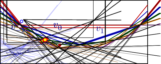
Figure 3.2: When computing the top $k$ levels, we might not know (the degree, and thus) the level of a vertex that is on the bottommost $k$-upper level, such as the arrow-marked vertex. We do know, though, the level of any vertex, like the circle-marked vertex, that lies strictly above the $k$-upper level.

To recap, we have shown that in Case (i) we can find all the maximum-level vertices in $O(n\log n)$ time.

Case (ii).

Here we first retrieve, in $O(n)$ time, the single vertex $v$ of the upper envelope and the set $L_{v}$ of all its incident lines. We obtain the corresponding sets $L_{v}^{-}$, $L_{v}^{+}$ of their left and right rays, respectively, and sort each of them in descending order, as prescribed earlier. We take the complementary set $K=L\setminus L_{v}$, compute its upper envelope $E_{K}$, and test each ray of $L_{v}^{-}\cup L_{v}^{+}$ for intersection with $E_{K}$. All this takes $O(n\log n)$ time, and yields the parameter $D$.

We compute the parameters $h$, $D_{0}$, as defined in Section 1, and remove from $L$ the $h$ lines that contribute the $h$ topmost rays to $L_{v}^{-}$ and the $h$ lines that contribute the $h$ topmost rays to $L_{v}^{+}$. We then compute the at-most-$4\log n$-upper level in the arrangement ${\cal A}(L_{0})$ of the set $L_{0}$ of the surviving lines, and report all vertices of maximum level (in ${\cal A}(L_{0})$), as we did in Case (i). We claim that these are also the maximum-level vertices in ${\cal A}(L)$. Indeed, this follows from the construction, observing that (a) for any such vertex $u$, other than $v$, the number of lines of $L$ that pass above $u$ is exactly $h$ plus the number of lines of $L_{0}$ that pass above $u$, (b) these upper levels do not contain any vertex of ${\cal A}(L)$ that is not a vertex of ${\cal A}(L_{0})$, and (c) for any other point $u$ that lies below these upper levels, the number of lines of $L$ that pass above $u$ is at least $h$ plus the number of lines of $L_{0}$ that pass above $u$.

That is, we have shown that in Case (ii) too we can find all the maximum-level vertices in $O(n\log n)$ time. In summary, we have finally managed to solve Exercise 8.13 in [dBCKO08] for the case where all the input lines are distinct. That is, we have:

Theorem 3.1.

All the maximum-level vertices in an arrangement of $n$ distinct lines in the plane can be computed in $O(n\log n)$ time.

4 The case of coinciding lines

We now turn to the more degenerate setup where the lines of $L$ can repeat themselves. Let $\Gamma=\{\gamma_{1},\ldots,\gamma_{m}\}$ be the set obtained from $L$ by removing duplicates. The lines of $\Gamma$ are pairwise distinct, and we denote by $f$ the function that maps each line in $L$ to its representative (overlapping) line in $\Gamma$. For each $\gamma\in\Gamma$ we denote by $\mu(\gamma)$ its multiplicity, namely the number of lines $\ell\in L$ satisfying $f(\ell)=\gamma$. We naturally have $\sum_{\gamma\in\Gamma}\mu(\gamma)=n$.

The level $\lambda_{\Gamma}(p)$ of a point $p$ in ${\cal A}(\Gamma)$ is defined, as before, to be the number of lines of $\Gamma$ that pass strictly below $p$. The situation is somewhat different for ${\cal A}(L)$. For any point $p$ in the plane define

$$S(p):=\sum_{\gamma\in\Gamma\,:\,\gamma\text{ passes below }p}\mu(\gamma).$$

If $p$ is a vertex of ${\cal A}(L)$ then its level in ${\cal A}(L)$ is $\lambda_{L}(p)=S(p)$. If $p$ lies in the relative interior of an edge of ${\cal A}(L)$ then it lies on some line $\gamma$ of ${\cal A}(\Gamma)$, and we say that $p$ lies at level $k$ in ${\cal A}(L)$ if

$$S(p)\leq k<S(p)+\mu(\gamma).$$ (4.1)

In words, an edge $e$ of ${\cal A}(L)$ (that is, of ${\cal A}(\Gamma)$) may participate in several consecutive levels, depending on its multiplicity. This extends to edges a similar phenomenon (already noted) that holds only for vertices in arrangements of distinct lines.

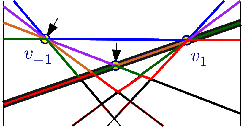
Input lines	Upper level 0	Upper levels 0 & 1	Upper levels 0–2 .
Upper levels 0–3	Upper levels 0–4	Upper levels 0–5	Upper levels 0–6 .

Figure 4.1: The thick line has multiplicity $2$, all other lines have multiplicity $1$. Upper level 4 is the first upper level that has detached vertices above it, marked by arrows in the sixth subfigure.

The $k$-level $\Lambda^{\downarrow}_{k}$ in ${\cal A}(L)$ is the closure of the union of all edges $e$ of ${\cal A}(\Gamma)$ that lie at level $k$ (in ${\cal A}(L)$, according to the definition in Eq. (4.1)). Fully symmetric definitions apply to the upper level. See Figure 4.1 for an illustration. Note that, as in the case of distinct lines (and even more so in this setup), the level does not necessarily turn at every vertex $v$ that it reaches: it could pass through $v$ staying on the same line of $\Gamma$; see for example upper levels 2, 3 and 4 in Figure 4.1 for an illustration. Note also that in this setup different levels may share edges of ${\cal A}(\Gamma)$.

As in the case of distinct lines, we wish to find the smallest upper level $k_{0}$ in ${\cal A}(L)$ for which there is a vertex in ${\cal A}(L)$ that lies strictly above $\Lambda^{\uparrow}_{k_{0}}$. All these (detached) vertices will be our desired maximum-level vertices, a property that is established rigorously in the following lemma.

Lemma 4.1.

Let $k_{0}$ be the first index for which ${\cal A}(L)$ contains a vertex that lies strictly above the $k_{0}$-upper level $\Lambda^{\uparrow}_{k_{0}}$ of ${\cal A}(L)$. Then all these ‘detached’ vertices (and only those) are the maximum-level vertices of ${\cal A}(L)$.

Proof. Let $v$ be one of these detached vertices. We have $\lambda_{L}(v)=\mu(e)+S(e)$, where $e$ is the edge of $\Lambda^{\uparrow}_{k_{0}}$ within ${\cal A}(\Gamma)$ lying vertically below $v$, and $\mu(e)$ (resp., $S(e)$) is the value $\mu(p)$ (resp., $S(p)$) for any point $p\in e$. If $v$ lies vertically above a vertex of $\Lambda^{\uparrow}_{k_{0}}$, apply this definition to an edge $e$ of $\Lambda^{\uparrow}_{k_{0}}$ incident to this vertex. By definition, and since $k_{0}$ is the smallest upper level with this property, we have $\lambda_{L}(v)=n-k_{0}$. On the other hand, let $w$ be any vertex lying on or below $\Lambda^{\uparrow}_{k_{0}}$. Assume for simplicity that $w$ is a vertex of $\Lambda^{\uparrow}_{k_{0}}$. Move, as before, from $w$ to a point $w^{\prime}$ slightly to the left of $w$ along the line of $L$ that lies on $\Lambda^{\uparrow}_{k_{0}}$ just to the left of $w$. Any line (of $L$) that passes strictly below $w$ also passes below $w^{\prime}$, so, again by definition, $\lambda_{L}(w)\leq\lambda_{L}(w^{\prime})<\mu(e)+S(e)=n-k_{0}$, where $e$ is the edge of ${\cal A}(L)$ (or rather of ${\cal A}(\Gamma)$) that contains $w^{\prime}$. The same argument applies to vertices $w$ below $\Lambda^{\uparrow}_{k_{0}}$; the level $\lambda_{L}(w)$ can only get smaller. $\Box$

Due to the non-standard definition of levels in ${\cal A}(L)$, it seems difficult (and at the moment we do not know how) to apply the method of the previous sections to the current setting. Instead we proceed as follows. We first perturb the lines in $L$ to obtain a set of lines $\hat{L}$, which induces a degeneracy-free arrangement ${\cal A}(\hat{L})$. We then work in tandem with both this perturbed arrangement, and the arrangement ${\cal A}(\Gamma)$. We use the arrangement ${\cal A}(\hat{L})$ to carry out a binary search on its upper levels. Each time we extract a specific $k$-upper level from ${\cal A}(\hat{L})$, we transform it into a polygonal curve $\pi_{k}$, which is contained in the union of the lines of $\Gamma$, and which is precisely the $k$-upper level of ${\cal A}(L)$, as defined above. We look for the smallest $k$ for which there is at least one vertex in ${\cal A}(\Gamma)$ strictly above $\pi_{k}$. In the remainder of this section we describe the perturbation of the lines of $L$ into those of $\hat{L}$, how we carry out the binary search over the upper levels of ${\cal A}(\hat{L})$, and how we detect whether, for a given $k$, there is a vertex of ${\cal A}(\Gamma)$ above $\pi_{k}$.

The perturbation.

We apply symbolic perturbation to the lines in $L$, using the parallel shifting mechanism described in Section 3, to obtain the set $\hat{L}=\{\hat{\ell}_{1},\ldots,\hat{\ell}_{n}\}$. Notice that this turns each line $\gamma\in\Gamma$ into $\mu(\gamma)$ parallel lines, infinitesimally close to one another. We define another function $F$, which maps each perturbed line $\hat{\ell}_{i}$ to the line $\gamma_{j}\in\Gamma$ that overlaps with the original line $\ell_{i}$ whose perturbed counterpart is $\hat{\ell}_{i}$, namely $F(\hat{\ell}_{i})=f(\ell_{i})$.

Notice that, under the standard conventions about symbolic perturbation, the arrangement ${\cal A}(\hat{L})$ is in general position (except for lines overlapping the same $\gamma\in\Gamma$ being parallel to one another). We compute the $k$-upper level $\Lambda^{\uparrow}_{k}$ of ${\cal A}(\hat{L})$, using a standard procedure for this task (see [EW86] and the appendix), and then transform it into the aforementioned unbounded $x$-monotone polygonal curve $\pi_{k}$, comprising non-infinitesimal portions (segments and rays) of the lines in $\Gamma$, joined together at the infinitesimal gaps between them (when such gaps exist); see Figure 4.2. This is done exactly as in the procedure in Section 3 for extracting the unperturbed level in degenerate arrangements that have no coinciding lines.

(a) (b) (c) (d) (e)

Figure 4.2: The construction of $\pi_{k}$ near a vertex, for $k=3$. (a) The input lines with their multiplicities. (b) The perturbed lines, and the level in the perturbed arrangement. (c) The path $\pi_{k}$ in ${\cal A}(\Gamma)$ – six infinitesimal edges have been deleted. (d) Another example of a level,now for $k=4$ and (e) its resulting path $\pi_{k}$ in the arrangement ${\cal A}(\Gamma)$.

The binary search for computing $k_{0}$.

To compute $k_{0}$ and the set $V_{0}$ of the detached vertices, we perform a binary search over the upper levels in ${\cal A}(\hat{L})$ in the following manner. Initially the range of potential levels is $[1,n]$ and we set $k$ to be $\lfloor n/2\rfloor$. We compute the $k$-upper level $\Lambda^{\uparrow}_{k}$ of ${\cal A}(\hat{L})$ (see below for details), and transform $\Lambda^{\uparrow}_{k}$ into $\pi_{k}$ as described above. We then compute the portions of the lines in $\Gamma$ that lie above $\pi_{k}$ (see details below). Again, this is a collection of line segments and rays, which we denote by $\Delta_{k}$. We now need to determine whether any pair of elements of $\Delta_{k}$ intersect strictly above $\pi_{k}$ (i.e., they intersect at their relative interiors), which we can do using the decision procedure to be described below. If there is no such intersection, then the current $k$ is too small, and the new range is the bottom half of the current range, otherwise we set the new range to be the top half. We set $k$ to be the middle index of the new range and recurse. It may be the case that we do not find a desired level with a vertex above it, in which case the maximum level of any vertex of ${\cal A}(\Gamma)$ is zero; this can only happen if all the lines meet in a single point, which is the single vertex of the arrangement.

To complete the description of the algorithm, we detail two procedures, which will be applied at each step of the binary search, for: (i) finding the set $\Delta_{k}$ of segments and rays that lie above $\pi_{k}$, and (ii) deciding whether the curves in $\Delta_{k}$ intersect above $\pi_{k}$. Also, we describe how to find the set of vertices $V_{0}$, once the level $k_{0}$ had been determined.

Computing the set $\Delta_{k}$.

In order to determine whether there is a vertex of the arrangement ${\cal A}(L)$ above $\pi_{k}$, we first need to collect the portions of lines in $\Gamma$ that lie above $\pi_{k}$, To do so, we find the leftmost vertex of the arrangement $\mathcal{A}(\Gamma)$ in $O(n\log n)$ time and project it vertically onto $\pi_{k}$. We then add a breakpoint $b_{L}$ along $\pi_{k}$ slightly to the left of this projection point and substitute the portion of the ray of $\pi_{k}$ emanating from $b_{L}$ to the left by the upward vertical ray from $b_{L}$. We apply a symmetric modification at the rightmost vertex of $\mathcal{A}(\Gamma)$, and replace the right ray of $\pi_{k}$ with the segment connecting the rightmost vertex of $\pi_{k}$ with the new point $b_{R}$ along $\pi_{k}$ and an upward vertical ray from $b_{R}$.

Denote this modified version of $\pi_{k}$ by $\pi^{\prime}_{k}$. We now compute the set $\Delta_{k}$ of line segments comprising all the portions of lines of $\Gamma$ that lie above $\pi^{\prime}_{k}$, each represented by its left and right endpoints. (Notice that, since we use the modified version $\pi^{\prime}_{k}$, the set $\Delta_{k}$ contains segments only, and no rays.) We intersect the lines in $\Gamma$ with the upward vertical ray from $b_{L}$, to obtain some of the left endpoints of segments in $\Delta_{k}$ (which are in fact internal points on the corresponding original rays). We store these endpoints in an array $W$, which has an entry (not always occupied) for every line in $\Gamma$. Initially we set $W[\ell]$:=null for every line $\ell\in\Gamma$. Additional endpoints are detected by moving along $\pi^{\prime}_{k}$ from left to right and carefully examining, for each vertex $v$ of the original $\pi_{k}$, the set $\Gamma(v)$ of all the lines of $\Gamma$ that are incident to $v$.

To determine $\Gamma(v)$, we consider the (one or two) lines that contain the edges of $\pi_{k}$ incident to $v$, together with all the infinitesimal edges that have been produced as part of $\Lambda^{\uparrow}_{k}$ within $\mathcal{A}(\hat{L})$, and have been collapsed to $v$. Consider such an infinitesimal edge $e$. Let $\hat{\ell}_{e}$ be the perturbed line containing $e$, and let $v$ be the vertex of $\pi_{k}$ to which $e$ will be contracted during the process of constructing $\pi_{k}$ (which may in particular unite two collinear segments into a common segment). The line $f(\hat{\ell}_{e})$ is split by $v$ into a leftward and a rightward ray. Consider the leftward ray, and compare its slope with that of the line supporting the edge $g$ immediately to the left of $v_{k}(e)$ along $\pi_{k}$. If the ray has a smaller slope than $g$, then $v_{k}(e)$ is the right endpoint of a segment whose left endpoint is stored in $W$. We add this segment to $\Delta_{k}$ and remove the corresponding entry from $W$. For the rightward ray we compare its slope with the slope of the line containing the edge $h$ along $\pi_{k}$ immediately to the right of $v_{k}(e)$. If it has a larger slope than the line containing $h$, then we insert $v_{k}(e)$ into $W$ at the entry for $f(\hat{\ell}_{e})$, as this is the left endpoint of a segment that will eventually be added to $\Delta_{k}$. (Notice that $f(\hat{\ell}_{e})$ may contribute to $\Delta_{k}$ two segments incident to $v$.) Finally we intersect the upward vertical ray from $b_{R}$ with each of the lines in $\Gamma$ and using $W$ we form the corresponding segments (representing right rays) and add them to $\Delta_{k}$.

Since we are using the infinitesimal edges of $\mathcal{A}(\hat{L})$, we may encounter a segment of $\mathcal{A}(\Gamma)$ that should be added to $\Delta_{k}$ several times (as many times as its multiplicity)). We wish to report each such segment only once. To do so, for any line $\ell$ of $\Gamma$ we only insert a left endpoint to $W[\ell]$ if this entry is null, namely it does not currently contain a left endpoint (if it already contains a left endpoint, this means that the left endpoint of this specific segment has already been detected due to another copy of $\ell$ in $\hat{L}$). Similarly, when we detect a right endpoint of a segment, we only report the segment if $W[\ell]$ contains a left endpoint—in that case we add the segment having these endpoints (the left endpoint in $W[\ell]$ and the corresponding right endpoint that we have just detected) to $\Delta_{k}$ and set $W[\ell]$ to null.

This process of constructing the set $\Delta_{k}$ takes time proportional to the complexity of the weighted $k$th level of $\mathcal{A}(\hat{L})$, where each vertex of the level is counted as many times as there are lines passing through it. We show in Lemma 5.1 in the next section that this quantity is bounded by $O(nk^{1/3})$. This also bounds the size $|\Delta_{k}|$ of $\Delta_{k}$.

Deciding whether there is a vertex of the arrangement ${\cal A}(\Gamma)$ strictly above $\pi_{k}$.

We run a sweep-line algorithm over the segments in $\Delta_{k}$, to detect the first intersection that does not lie on $\pi_{k}$. Notice that all the vertices of $\pi_{k}$ are inserted into the event queue before the sweep starts. Such vertices occur at common endpoints of the segments, and are not intersections that we seek (which only occur within the relative interior of the segments). The same holds for the intersection of lines in $\Gamma$ with either $b_{L}$ or $b_{R}$—we insert them to the queue before the sweep starts and neither set contains a relevant vertex of the type we are looking for.

Finding the set $V_{0}$ of detached vertices.

After terminating the binary search at some index $k_{0}$, we need to find the set $V_{0}$ of all detached vertices above $\pi_{k_{0}}$. We consider the set $\Delta_{k_{0}}$ of segments, and observe that all the vertices in $V_{0}$ are vertices of the lower envelope of $\Delta_{k_{0}}$. Indeed, no segment of $\Delta_{k_{0}}$ can lie below any vertex $v$ of $V_{0}$, for then $v$ would be detached from an upper level with a smaller index. We thus need to compute the lower envelope, which we can do using a standard divide-and-conquer technique (see, e.g., [SA95]). Since $|\Delta_{k_{0}}|=O(nk_{0}^{1/3})$, this construction takes $O(nk_{0}^{1/3}\alpha(n)\log n)$ time. We output those vertices of the envelope that lie in the relative interiors of their incident segments (ignoring segment endpoints).

The overall complexity.

Computing the $k$-upper-level in ${\cal A}(\hat{L})$ takes $O(nk^{1/3}\log^{2}k)$ time [EW86] (see also the appendix). This time dominates the time of the other procedures carried out in a single step of the binary search. Hence, multiplying this by the number $O(\log n)$ of binary search steps, we thus conclude:

Theorem 4.2.

The maximum-level vertices in an arrangement of $n$ lines, where some lines may coincide, can be computed in $O(n^{4/3}\log^{3}n)$ time.

Remark. We can modify the binary search so that it first runs an exponential search from the top of the arrangement, and only reverts to standard binary search at the first time when the current level exceeds $k_{0}$. This improves the running time to $O(nk_{0}^{1/3}{\rm polylog}\;n)$, when $k_{0}\ll n$. Obtaining such a sharp bound on $k_{0}$, or giving a construction in which $k_{0}=\Theta(n)$, remains one of the open problems raised by the present work.

5 The complexity of the weighted $k$-level in degenerate arrangements

Finally, we consider a related combinatorial question for degenerate arrangements. The resulting combinatorial bound, stated in Lemma 5.1, has been used in the analysis of the previous section.

As before, let $L$ be a set of $n$ lines, not necessarily in general position: we allow many lines to intersect in a single point, but assume that all the lines are distinct. Recall that the vertices of the $k$th level $\Lambda^{\downarrow}_{k}$ are not necessarily at level $k$. As a matter of fact, as already noted, if the degree of a vertex $v$ of ${\cal A}(L)$ is $d$ and $k$ lines pass below $v$, then $v$ belongs to the $d$ consecutive levels $k,k+1,\ldots,k+d-1$ of ${\cal A}(L)$. Let $|\Lambda^{\downarrow}_{k}|$ denote the complexity of $\Lambda^{\downarrow}_{k}$, that is, the number of its vertices, and let $\omega(\Lambda^{\downarrow}_{k})$ denote the weighted complexity of $\Lambda^{\downarrow}_{k}$, defined as the sum of the degrees of the vertices of $\Lambda^{\downarrow}_{k}$. It is known [Dey98] that $|{\Lambda^{\downarrow}_{k}}|=O(nk^{1/3})$ in the non-degenerate case (for this case we have $\omega(\Lambda^{\downarrow}_{k})=2|\Lambda^{\downarrow}_{k}|$). We strengthen this result for the degenerate case in the following lemma.

Lemma 5.1.

Let $L$ be a set of $n$ distinct lines in the plane, not necessarily in general position. Then $\omega(\Lambda^{\downarrow}_{k})=O(nk^{1/3})$.

Proof. We convert the original arrangement of lines into an arrangement of pseudo-lines in general position, by making local changes in the vicinity of every vertex of degree greater than two. Furthermore, we ensure that, in the new arrangement, when the $k$th level passes through the vicinity of any original vertex $v$ (so $v$ is a vertex of the original level), it visits all the pseudo-lines whose original lines pass through $v$, each along some segment thereof, before leaving this neighborhood.

Consider such an original vertex $v$, of some degree $d=d(v)\geq 3$ (vertices of degree two require no action); see Figure 5.1(a). The $k$th level enters this vertex from the left, say on a line $\ell_{L}$, and leaves to the right, say on a line $\ell_{R}$. Assume that $\Lambda^{\downarrow}_{k}$ forms a right turn at $v$ (the left turn case is handled in a similar fashion to what is described below, and it may also be the case that there is no turn, and the level enters and leaves $v$ along the same line). A line that reaches $v$ from the left below the level, and leaves $v$ to the right above the level, is called ascending, a line that reaches $v$ from the left above the level but leaves $v$ to the right below the level is called descending, and a line that does neither is called neutral; such lines stay on the same side of the level both to the left and to the right of $v$. In particular, $\ell_{L}$ and $\ell_{R}$ are neutral. Under the right-turn assumption, all the neutral lines pass above or on the level, both to the left and to the right of $v$; see Figure 5.1(a).

We deform the batch of ascending lines into the kink-like structure $K_{a}$, and the batch of descending lines into the kink-like structure $K_{d}$, as depicted in Figure 5.1(b). We make the two middle portions of the kinks cross one another to the left of $v$, and below the (still untouched) batch of neutral lines. The lines of each class remain pairwise disjoint in a suitable small neighborhood $\Omega$ of the crossing, but we make every pair of them cross in some other portion of the respective kink, to the right of $\Omega$ and away from the lines of the other two classes.

In addition, we deform the neutral lines within another small neighborhood $\Omega^{\prime}$ of $v$ that is disjoint from any ascending or descending line (and from $\Omega$), so that each of them contributes an arc (of nonzero length) to their lower envelope within $\Omega^{\prime}$.

The construction ensures that the $k$th level in the modified scenario proceeds along $\ell_{L}$ until it reaches $K_{d}$, then turns right along the first (leftmost) descending line, reaches $\Omega$, traces a zigzag pattern, alternating between ascending lines and descending lines, leaves $\Omega$ along the rightmost ascending line (this follows since the number of ascending lines is equal to the number of descending lines), reaches $\ell_{L}$ again, and then proceeds along $\ell_{L}$ until it enters $\Omega^{\prime}$; see the left magnifying glass in Figure 5.1(b). The deformation within $\Omega^{\prime}$ ensures that the level traces the lower envelope of the neutral lines, and leaves $\Omega^{\prime}$ along $\ell_{R}$; see the right magnifying glass in Figure 5.1(b).

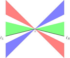
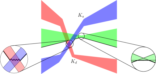
(a)              (b)

Figure 5.1: (a) The lines passing through the original vertex $v$, with the $k$th level marked in black. The ascending lines are marked in blue, the descending lines in red, and the neutral lines in green. (b) The vicinity of the vertex $v$ after the local transformation of the lines into pseudo-lines, where the neighborhoods $\Omega$ (to the left) and $\Omega^{\prime}$ (to the right) are magnified.

The above transformation can be performed by deforming the lines incident to $v$ only within an arbitrarily small square around $v$, disjoint from all other vertices and their surrounding squares, so that the new curves coincide with the original lines on the boundary of and outside this square. By construction, inside this square every pair of modified curves intersect at exactly one point, and none of these pairs intersect outside the square (even after the local perturbations taking place at square neighborhoods of other vertices). Hence the curves that come from the original lines that are incident to $v$ constitute a family of pseudo-lines. We repeat this deformation for every vertex $v$ of the $k$th level of degree greater than $2$. For vertices $v$ that are not on the level, whose degree is greater than $2$, a simpler deformation suffices, only ensuring that each pair of lines that are incident to $v$ intersect now, after their perturbations, at a distinct point, within a sufficiently small neighborhood of $v$. All this results in a collection of $n$ pseudo-lines in general position, so that, for every vertex $v$ of $\Lambda^{\downarrow}_{k}$, each line incident to $v$ now contributes at least one edge to the $k$th level of the modified arrangement, within the square corresponding to (and surrounding) $v$.

We have thus constructed an arrangement of pseudo-lines so that the complexity of its $k$th level is at least proportional to $\omega(\Lambda^{\downarrow}_{k})$. By the result of Tamaki and Tokuyama [TT03], the complexity of the $k$th level in an arrangement of $n$ pseudo-lines is $O(nk^{1/3})$. This completes the proof. $\Box$

Acknowledgments.

The authors thank Michal Kleinbort and Shahar Shamai for pointing out the difficulty of the problem of finding the maximum-level vertex.

Work by Dan Halperin has been supported in part by the Israel Science Foundation (grants no. 825/15 and 1736/19), by the Blavatnik Computer Science Research Fund, and by grants from Yandex and from Facebook.

Work by Sariel Har-Peled was supported by an NSF AF award CCF-1907400.

Work by Micha Sharir has been supported in part by Grant 260/18 from the Israel Science Foundation, by Grant G-1367-407.6/2016 from the German-Israeli Foundation for Scientific Research and Development, and by the Blavatnik Computer Science Research Fund.

Appendix A A review of a variant of the algorithm of Everett et al.

In this appendix we present a variant of the algorithm by Everett et al. [ERK96] for constructing the top $k$ levels of an arrangement of lines.

Theorem A.1.

(Based on Everett et al. [ERK96]) Given a set $L$ of $n$ lines in general position in the plane, and a parameter $k$, one can compute the top $k$ levels of ${\cal A}(L)$ in $O(n\log n+nk)$ time.

Proof. We proceed in four steps. First, we discuss the case where all the lines of $L$ show up on the upper envelope and derive a point location data structure that we need in the other steps. In the second step, we compute $k$ sets of lines $L^{\prime}_{1},\ldots,L^{\prime}_{k}$ such that only lines in $L^{\prime}:=L^{\prime}_{1}\cup\cdots\cup L^{\prime}_{k}$ appear in the $k$ top levels of ${\cal A}(L)$. Next we compute the $k$th upper level of ${\cal A}(L^{\prime})$, making use of the decomposition computed in step 2 and the data structure derived in step 1. Finally, we compute the part of the arrangement of ${\cal A}(L^{\prime})$ lying on or above the $k$th upper level.

Let $L$ be a set of $n$ lines in the plane in general position, meaning that no point is incident to more than two lines of $L$ ($L$ may contain parallel lines). Consider the special case where all the lines of $L$ show up on the upper envelope $E$ of $L$. Then ${\cal A}(L)$ has a special structure: except for the top face, which is bounded by all $n$ lines, and the bottom face and the two unbounded faces adjacent to the top face, which are wedges bounded by only two lines, every other face is either a triangle or a quadrangle. The triangles are all the other unbounded faces and all the other faces adjacent to the top face, and the quadrangles are all the other faces. See Figure A.1(left).

Point location in this arrangement is simple. We compute $E$, in $O(n\log n)$ time (this amounts, in the special case under consideration, to just sorting the lines of $L$ by their slopes). Then, given a query point $q$ below $E$, we can compute the face of ${\cal A}(L)$ containing $q$ in $O(\log n)$ time. The simplest way of doing this is to compute the (at most) two tangents from $q$ to $E$, and use only the (at most four) lines incident to the points of tangency to compute the desired face. See Figure A.1(right).

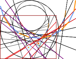
Figure A.1: The special structure of the arrangement of lines that are in “convex” position, meaning that they all show up on their upper envelope. Left: The arrangement. Right: Locating a point below the envelope.

Consider now the general case, where we are given an arbitrary set $L$ of $n$ lines in general position, and a parameter $k$, and we want to construct the $k$ top levels of ${\cal A}(L)$. We apply the following iterative ‘peeling’ process to $L$, to obtain a sequence $L_{1},L_{2},\ldots,L_{k}$ of subsets of $L$. We set $L_{1}=L$ and, for each $i\geq 1$, we obtain $L_{i+1}$ from $L_{i}$ by constructing the upper envelope $E_{i}$ of ${\cal A}(L_{i})$, defining $L^{\prime}_{i}$ to consist of all the lines that show up on the envelope, and setting $L_{i+1}:=L_{i}\setminus L^{\prime}_{i}$. A naive implementation of this process takes $O(k\cdot n\log n)=O(nk\log n)$ time, but we can improve it to $O(nk+n\log n)$ by noting that, once the lines of $L$ are sorted by slope, we can compute the upper envelope (of any prescribed subset of $L$) in linear time, e.g., by a dual version of Graham’s scan algorithm for computing convex hulls (see, e.g., [dBCKO08]). Set $L^{\prime}:=L^{\prime}_{1}\cup\cdots\cup L^{\prime}_{k}$. By construction, only the lines of $L^{\prime}$ appear in (i.e., support the edges of) the $k$ top levels of ${\cal A}(L)$.

In the next step, we construct the $k$th upper level of ${\cal A}(L^{\prime})$ by tracing it from left to right. Finding the leftmost edge (ray) of the level is easy to do in linear time. Suppose that we are currently at some point $q$ on some edge $e$ of the level, and let $i$ be the index for which the line $\ell$ containing $e$ belongs to $L^{\prime}_{i}$. The right endpoint $q^{\prime}$ of $e$ is the nearest intersection of the rightward-directed ray emanating from $q$ along $e$ with another line of $L^{\prime}$. We find $q^{\prime}$ using the dynamic half-space intersection data structure of Overmars and van Leeuwen [OvL81]. This data structure maintains the intersection of half-spaces under insertions and deletions and supports ray-shooting queries from any point inside the intersection. The intersection must be non-empty at all times and the ray-shooting query returns the half-space first hit by the ray. We use the data structure as follows: For each $j\neq i$, the face of ${\cal A}(L^{\prime}_{j})$ that contains $q$ contributes the at most four half-spaces defining the face. For $L^{\prime}_{i}$, $e$ bounds two faces of ${\cal A}(L^{\prime}_{i})$, the union of which is defined by at most four half-spaces in $L^{\prime}_{i}$. We maintain the collection of the at most $4k$ such half-spaces. Each ray-shooting query takes $O(\log^{2}k)$ time and half-spaces can be added and removed in the same time bound.

After we obtain $q^{\prime}$, the new edge $e^{\prime}$ that the level follows lies on the new line $\ell^{\prime}$ containing $q^{\prime}$ (note that $\ell^{\prime}$ is unique since our lines are assumed to be in general position); let $j$ be the index for which $\ell^{\prime}\in L^{\prime}_{j}$. Consider the case $i\neq j$; the case $i=j$ is easier to handle. For every index $m\neq i,j$, both $q$ and $q^{\prime}$ lie in the same face of ${\cal A}(L^{\prime}_{m})$, so the at most four lines of $L^{\prime}_{m}$ that are stored in the structure do not change. For $L^{\prime}_{i}$, $e^{\prime}$ enters one of the two faces of ${\cal A}(L^{\prime}_{i})$ adjacent to $e$. We insert $\ell$ into the structure and delete the opposite line bounding the other face. For $L^{\prime}_{j}$, we are now tracing (along $e^{\prime}$) the common boundary of two faces. We delete $\ell^{\prime}$ from the structure and insert the line bounding the opposite edge of the new face.

That is, each new vertex on the $k$th level takes $O(\log^{2}k)$ time to obtain. Since the complexity of the $k$th (upper) level in an arrangement of $n$ lines (in general position) is $O(nk^{1/3})$ [Dey98], the total cost of constructing the level is $O(nk^{1/3}\log^{2}k)$.

In conclusion, one can compute the $k$th upper level $\Lambda^{\uparrow}_{k}$ of ${\cal A}(L)$ in $O(n\log n+nk+nk^{1/3}\log^{2}k)=O(n\log n+nk)$ time.

We come to the final step. We construct the lower convex hull $C_{k}$ of $\Lambda^{\uparrow}_{k}$, which can be done in linear time, that is, in $O(nk^{1/3})$ time, since the vertices of $\Lambda^{\uparrow}_{k}$ are already sorted from left to right. Note that each point $q$ on or above $C_{k}$ lies at upper level at most $2k$, because every line that passes above $q$ must pass above at least one of the two endpoints of the edge of $C_{k}$ that contains $q$ or passes below $q$. For each line $\ell\in L$ we compute its (one or two) intersection points with $C_{k}$, in $O(\log n)$ time, and thereby obtain its portion above $C_{k}$. The overall time for this step is $O(n\log n+nk^{1/3})$.

Let $S$ denote the resulting collection of at most $n$ segments and rays. Since all the elements of $S$ are contained in the at-most-$2k$ upper level of ${\cal A}(L)$, the complexity of ${\cal A}(S)$ is $O(nk)$ (see [AG86]). We construct ${\cal A}(S)$ using the deterministic algorithm of Chazelle and Edelsbrunner [CE92], which runs in $O(n\log n+nk)$ time. Alternatively, we can use the randomized incremental algorithm described in [dBCKO08], which runs in expected time $O(n\log n+nk)$. Finally, we sweep ${\cal A}(S)$ once more to remove any vertex or edge of the arrangement that lies below $\Lambda^{\uparrow}_{k}$. This step can also be performed in $O(n\log n+nk)$ time, by traversing the planar map obtained from the previous construction, updating the level in $O(1)$ time when we cross from one feature to an adjacent one. $\Box$

References

- [AG86] N. Alon and E. Győri. The number of small semispaces of a finite set of points in the plane. J. Combin. Theory Ser. A, 41:154–157, 1986.
- [CE92] B. Chazelle and H. Edelsbrunner. An optimal algorithm for intersecting line segments in the plane. J. Assoc. Comput. Mach., 39:1–54, 1992.
- [CS89] K. L. Clarkson and P. W. Shor. Applications of random sampling in computational geometry, II. Discrete Comput. Geom., 4(5):387–421, 1989.
- [dBCKO08] M. de Berg, O. Cheong, M. van Kreveld, and M. H. Overmars. Computational Geometry: Algorithms and Applications. Springer-Verlag, Santa Clara, CA, USA, 3rd edition, 2008.
- [Dey98] T. K. Dey. Improved bounds for planar -sets and related problems. Discrete Comput. Geom., 19(3):373–382, 1998.
- [ERK96] H. Everett, J.-M. Robert, and M. van Kreveld. An optimal algorithm for the -levels, with applications to separation and transversal problems. Int. J. Comput. Geom. Appl., 6(3):247–261, 1996.
- [EW86] H. Edelsbrunner and E. Welzl. Constructing belts in two-dimensional arrangements with applications. SIAM J. Comput., 15(1):271–284, 1986.
- [HS18] D. Halperin and M. Sharir. Arrangements. In J. E. Goodman, J. O’Rourke, and Cs. D. Tóth, editors, Handbook of Discrete and Computational Geometry, chapter 28, pages 723–762. Chapman & Hall/CRC, Boca Raton, FL, 3rd edition, 2018.
- [OvL81] M. H. Overmars and J. van Leeuwen. Maintenance of configurations in the plane. J. Comput. Syst. Sci., 23:166–204, 1981.
- [SA95] M. Sharir and P. K. Agarwal. Davenport-Schinzel Sequences and Their Geometric Applications. Cambridge University Press, New York, 1995.
- [TT03] H. Tamaki and T. Tokuyama. A characterization of planar graphs by pseudo-line arrangements. Algorithmica, 35(3):269–285, 2003.