Deep Reinforcement Learning for Fresh Data Collection in UAV-assisted IoT Networks
Abstract
Due to the flexibility and low operational cost, dispatching unmanned aerial vehicles (UAVs) to collect information from distributed sensors is expected to be a promising solution in Internet of Things (IoT), especially for time-critical applications. How to maintain the information freshness is a challenging issue. In this paper, we investigate the fresh data collection problem in UAV-assisted IoT networks. Particularly, the UAV flies towards the sensors to collect status update packets within a given duration while maintaining a non-negative residual energy. We formulate a Markov Decision Process (MDP) to find the optimal flight trajectory of the UAV and transmission scheduling of the sensors that minimizes the weighted sum of the age of information (AoI). A UAV-assisted data collection algorithm based on deep reinforcement learning (DRL) is further proposed to overcome the curse of dimensionality. Extensive simulation results demonstrate that the proposed DRL-based algorithm can significantly reduce the weighted sum of the AoI compared to other baseline algorithms.
I Introduction
Owing to the fully controllable mobility and low operational cost, unmanned aerial vehicles (UAVs) emerge as promising technologies to provide wireless services [1]. One of the most important applications is to collect information from distributed sensors with the help of UAV in the Internet of Things (IoT). Since the UAV can fly close to each sensor and exploit the line-of-sight (LoS) dominant air-to-ground channel, the transmission energy of the sensors can be greatly reduced and the throughput of sensors can be significantly improved. Such advantages make UAV-assisted IoT networks attract extensive attention in recent years and arouse many research interests, ranging from the designs of UAV’s flight trajectory to resource allocation, and sensors’ wakeup schedule [2, 3, 4, 5, 6]. However, most of the existing works aimed at either maximizing system throughput or minimizing delay. Recently, the age of information (AoI) has been introduced to measure data freshness in IoT networks [7, 8, 9]. Particularly, AoI tracks the time elapsed since the latest received packet at the destination was generated at the source. In contrast to throughput and delay, the AoI metric is defined from the receiver’s perspective. Therefore, previous results in the literature can not be directly used to minimize the AoI in UAV-assisted IoT networks.
There have been some recent efforts on guaranteeing data freshness in UAV-aided data collection for IoT networks. In [10], the UAV was used as a mobile relay for a source-destination pair and the trajectory is designed to minimize the average Peak AoI. In an IoT network with multiple sensors, two age-optimal trajectory planning algorithms were proposed in [11], where the UAV flies to and hovers above each sensor to collect data. This work was then extended in [12], where the UAV collects data from a set of sensors when hovering at each collection point (CP). The sensor-CP association and the UAV’s flight trajectory were jointly designed to minimize the maximum AoI of the sensors. In a similar setup, an AoI deadline was imposed on each sensor and the UAV’s flight trajectory was designed to minimize the number of expired packets in [13]. In these works, however, the UAV collects the data of each sensor only once and then flies back to the depot. To continuously collect data packets during a period of time, the authors of [14] optimized both the UAV’s flight trajectory and the transmission scheduling of sensors to achieve the minimum weighted sum of AoI. Nonetheless, the energy consumption of the UAV has not been considered in the design of UAV’s age-optimal trajectory.
In this paper, by taking the energy constraint of UAV into consideration, we study the age-optimal data collection problem in UAV-assisted IoT networks based on deep reinforcement learning (DRL). In particular, a UAV is dispatched from a depot, flies towards the sensors to collect status update packets, and arrives at the destination within a given duration. The UAV has to maintain a non-negative residual energy while minimizing the weighted sum of the AoI of sensors during the flight. To find the optimal flight trajectory of the UAV and transmission scheduling of the sensors, we formulate this problem into a finite-horizon Markov decision process (MDP). Due to the high-dimensional state space, it is computationally prohibitive to solve the MDP problem using dynamic programming algorithms. To address this issue, we propose a DRL-based UAV-assisted data collection algorithm, where the UAV decides which direction to fly and which sensor to connect at each step. Extensive simulation results demonstrate that the proposed algorithm can significantly reduce the weighted sum of AoI compared to other baseline policies.
The rest of this paper is organized as follows: The system model and problem formulation are described in Section II. Section III provides the MDP formulation of the problem and presents the proposed DRL-based algorithm. The simulation results and discussions are given in Section IV. Finally, we conclude this paper in Section V.
II System Model and Problem Formulation
II-A Network Description
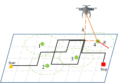
As shown in Fig. 1, we consider a UAV-assisted IoT network, where sensor nodes (SNs) are randomly distributed in a certain geographical region. The set of all the SNs is denoted by and the location of each SN is represented by for . The region of interest is equally partitioned into a number of small-size grids such that the UAV’s location is approximately constant within each grid. Moreover, the center of the -th grid is represented by . We denote by the set containing the locations of centers for all the grids. Moreover, the spacing distance between the centers of any two adjacent grids is denoted by .
We assume a discrete-time system where time is divided into equal-length time slots. The length of each slot is seconds. Given a time duration of slots, the rotary-wing UAV takes off from an initial location and flies over SNs to collect data packets. At the end of the -th slot, the UAV lands on a final destination . We assume that the UAV flies along the center of the grids at a fixed altitude . In each time slot, the UAV could hover over a certain grid or fly across one grid at a constant speed . Let denote the projection of the UAV’s location on the ground at time slot . Then, the projection of the UAV’s flight trajectory is defined as a sequence of center of grids , where and .
Let denote the initial amount of energy the UAV carries. The energy consumption of the UAV consists of the communication energy and the propulsion energy. Since the communication energy consumption is relatively small, we consider only the propulsion energy consumption in this paper. The propulsion energy of the rotary-wing UAV is mainly composed of the blade profile energy, the induced power, and the parasite energy [3]. The propulsion power consumption can be expressed as follows,
| (1) |
where and represent the blade profile power and derived power of the UAV in the hovering state, respectively, is the velocity of the UAV at slot , represents the tip speed of the rotor blade of the UAV, represents the mean rotor induced velocity in the hovering state, is the fuselage drag ratio, represents the density of air, indicates the rotor solidity, and represents the area of the rotor disk. In particular, the power consumption when hovering (i.e., ) is .
We assume that the UAV could establish the LoS links with the SNs due to its high attitude. Then, the channel power gain from the SN to the UAV at time slot can be given by
| (2) |
where is the channel gain at a reference distance of meter, denotes the Euclidean distance between the SN and the UAV at time slot . Let denote the transmission power of each SN. When the UAV is within the coverage of one SN, i.e., , the SN generates a status update of size and sends it to the UAV successfully in a time slot. Specifically, the coverage radius can be calculated as
| (3) |
where is the channel bandwidth, and is the noise power at the UAV.
We employ AoI to measure the freshness of information. In particular, the AoI is defined as the time elapsed since the generation of the latest status update received by the UAV. Let denote the time at which the latest status update of SN successfully received by the UAV was generated. The AoI of SN at the beginning of slot is then given by
| (4) |
Let be the vector of the SNs’ scheduling variables, where denotes which SN is scheduled to update its status at time slot . In particular, indicates that SN transmits to the UAV at slot and means that no transmission occurs at slot . According to (4), if SN is scheduled to transmit at slot and the UAV is located in the coverage of SN , then its AoI decreases to one; otherwise, the AoI increases by one. Then, the dynamics of the AoI can be given by
| (5) |
II-B Problem Formulation
Our objective is to find the optimal trajectory of the UAV and the optimal scheduling of the SNs that minimize the weighted average AoI of all the SNs. The optimization problem can be expressed as follows:
| (6) | ||||
| (7) | ||||
| (8) | ||||
| (9) |
where denotes the importance of SN . (7) ensures that the UAV will not run out of the energy before time slot . (8) and (9) guarantee that the UAV starts from the initial location and arrives at the final location at time slot . It is easily observed that the above optimization problem is a nonlinear integer programming one, which is computationally complex to solve for large-scale networks. In the following section, we propose a learning based algorithm for the UAV to learn its trajectory and the SNs’ transmission schedule at each location along the trajectory.
III DRL-based Approach
In this section, we first cast the UAV-assisted data collection problem into a Markov decision process (MDP) and then propose a DRL-based algorithm to minimize the weighted average AoI of all the SNs.
III-A MDP Formulation
We reformulate the problem P1 via an MDP, which is usually represented by a tuple . Here, presents the state, denotes the action, is the reward function, and is the state transition probability. MDP is commonly used to model a sequential decision-making process. In particular, at time slot , the agent observes some state and performs an action . After taking this action, the state of the environment transits to with probability , and the agent receives a reward . We consider the UAV as the agent for performing the data collection algorithm and define the state, action, and reward function in the following.
III-A1 State
The state at time slot is defined as , which is composed of four parts:
-
•
is the projection of the UAV on the ground at time slot .
-
•
is the AoI of all the SNs at the UAV at time slot . For the AoI of each SN, we have , where is the maximum value of AoI and can be chosen to be arbitrary large.
-
•
is the difference between the remaining time of the UAV and the minimum time required to reach the final destination.
-
•
is the difference between the remaining energy of the UAV and the energy required for the UAV to arrive at the final destination in the remaining time. , where is the set of the energy level of the UAV.
Altogether, the state space of the system can be expressed as .
III-A2 Action
The action of the UAV at time slot is characterized by its movement and the scheduling of SN , i.e., . In each time slot, the UAV either hovers at its current location or move to one of its adjacent cells. Specifically, . Then, the action space is given by .
III-A3 Reward
In our context of the UAV-assisted data collection, the reward should encourage the UAV to minimize the weighted average AoI of all the SNs under the constraints given by (7)-(9). When the UAV reaches the final destination at time slot with a non-negative residual energy, we will give the UAV an additional reward. However, a punishment will be imposed when the constraints are violated. Let . Then, the reward is defined as follows,
| (10) |
where , , and are positive constants and set large enough.
III-A4 State Transition
The AoI of each SN is updated as in (5). The dynamics of the UAV’s location can be expressed as
| (11) |
The time difference is updated based on the UAV’s location. In particular, if the UAV flies towards the final destination at slot , remains the same as . If the UAV hovers at slot , is decreased by one. While is decreased by two, if the UAV flies away from the final destination. Altogether, we can update as follows,
| (12) |
Since the power consumptions for hovering and flying are different, the update of energy difference is different for these two cases. According to the definition of the energy difference , the update of can be given by
| (13) |
Our goal is to find an age-optimal policy , which determines the sequential actions over a finite horizon of length . Given a policy , the total expected reward of the system starting from an initial state is defined as
| (14) |
Then, the optimal policy can be obtained by maximizing the total expected reward, i.e., . When the number of SNs become large, it is computationally infeasible to find the optimal strategy by standard dynamic programming method. Therefore, DRL is employed in the following subsection to solve this problem.
III-B DRL Approach
We employ DQN, which is one of the most well adopted DRL method, to derive the optimal policy. In this approach, we define a state-action value function , which represents the expected reward for selecting action in state and then following policy . The optimal Q-value function can be estimated by the update
| (15) |
where is the learning rate. The optimal policy is the one that takes the action which maximizes the Q-value function at each step.
By incorporating deep neural network (DNN) into the framework of Q-learning, DQN can overcome the curse of dimensionality. In particular, we use a DNN with weights to approximate the Q-value function with . The DNN can be trained by minimizing a sequence of loss function that changes at each slot . Specifically,
| (16) |
where the weights are updated at slot and the weight from the previous slot are held fixed. However, the use of one DNN may induce instability. In order to overcome this issue, two neural networks are employed [15], i.e., the current network with weights and the target network parameterized by . The current network is used as a function approximator and its weights are updated at every slot. While the target network computes the target Q-value function and its weights are fixed for a while and updated at every steps (Lines 11~18). In particular, the weights of the DNN are updated by minimizing the loss function, which is defined as
| (17) |
where is evaluated by the current network and is evaluated by the target network. Based on this, the update formula for weights is given as follows:
| (18) |
where and denotes the gradient with respect to .
Based on the DQN with two neural networks, the UAV-assisted data collection algorithm is proposed to find the optimal solution to problem P1, and the details are showed in Algorithm 1. At the beginning of the training process, the estimation of the Q-value function is far from accurate. Hence, the UAV should explore the environment more often at first. When the policy continues improving and the knowledge of the environment is more accurate, the UAV should exploit the learned knowledge more often. As such, we utilize a simple -greedy policy (Lines 6~7). In particular, the action is randomly selected to explore the environment with probability and the action that maximizes is chosen to exploit the policy with probability . Moreover, is set to be decreasing with the number of slots so that the UAV can choose the optimal action when the estimation of Q-value function converges.
Experience replay is used in the learning process. The agent stores the experience in the replay memory, and then samples a mini-batch of the experiences from the replay memory uniformly at random to train the neural network (Lines 9~10). By using experience replay, not only the correlation among the continuous samples is reduced, but also the utilization rate of the experience data can be improved. We also note that the UAV-assisted data collection problem we considered is episodic, since the UAV is required to be arrive in the final destination at time slot . In particular, there are three terminal cases: 1) when the UAV reaches the final destination at time slot , 2) when , and 3) when (Line 19).
IV Simulation Results
In this section, we perform extensive simulations to evaluate the performance of the DRL-based UAV-assisted data collection algorithm in an IoT network. We consider a square area of that is virtually divided into equally-sized grids of length m. Let the center of the left lower grid of the square region be the origin with coordinate and the index of every grid is the coordinate of the grid center divided by 25. For instance, the left lower grid is indexed by . We assume that UAV’s initial and final locations are at grids and , respectively. We also assume that the SNs have equal importance weights. Unless otherwise specified, the simulation parameters are presented in Table I.
The two neural networks in the proposed algorithm is implemented using Tensorflow. In particular, each DNN includes two fully-connected hidden layers with 200 and 256 neurons. The input layer size of the DNN is the same as the state space size and the output layer size of the DNN is equal to the total number of actions. The hypeparameters of DQN are summarized in Table II.
| Parameter | Value |
|---|---|
| Channel bandwidth | 1 MHz |
| Update size | 5 Mbits |
| Noise power | -100 dbm |
| Channel gain at m | -60 dB |
| Flight altitude | m |
| Time duration | 70 slots |
| UAV speed | 25 m/s |
| Initial energy | 2.2e4 J |
| Air density in | 1.225 kg/m3 |
| Tip speed | 120 m/s |
| Blade profile power | 99.66 W |
| Derived power | 120.16 W |
| Body resistance ratio | 0.48 |
| Robustness of the rotor | 0.0001 |
| The area of the rotor disk | 0.5 s2 |
| Mean rotor induced velocity in hover | 0.002 m/s |
| Parameter | Value |
|---|---|
| Episodes | 20000 |
| Reply memory size | 40000 |
| Mini-batch size | 200 |
| Initial | 0.9 |
| -greedy decrement | 0.0001 |
| Minimum | 0 |
| Learning rate | 0.002 |
| Learning rate decay rate | 0.95 |
| Learning rate decay step | 10000 |
| Update step | 300 |
| Optimizer | Adam |
| Activation function | ReLU |
In the following figures, we compare the performance of the proposed algorithm with two baseline algorithms, namely AoI-based algorithm and distance-based algorithm. In the AoI-based algorithm, the UAV flies to the SN with the largest AoI in the current time slot. While in the distance-based algorithm, the flight trajectory of the UAV is divided into multiple rounds. In each round, the UAV traverses all the SNs one by one and the UAV flies to the nearest and unvisited SN in the current traversal round. Moreover, the UAV can collect status update from the SNs on its way in both baseline algorithms. When the UAV’s residual energy or the remaining time is less than a threshold, it directly flies to the final destination.
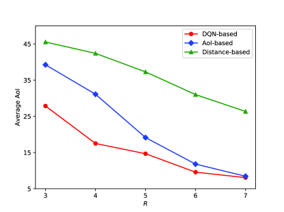
Fig. 2 illustrates the average AoI with respect to the coverage radius in a scenario with three randomly deployed SNs, where the value of is normalized by the length of a grid. From Fig. 2, we can see that a higher results in lower average AoI since it takes less time for the UAV to fly to collect data packets. Moreover, we can see that our proposed DQN-based algorithm outperforms the two baseline algorithms since it jointly considers the AoI, the location of the UAV, and the time and energy constraints. It is also shown that the AoI-based algorithm achieves almost the same performance as DQN-based algorithm when is large. This is because there is an overlap of the coverage of all the SNs for a larger and the UAV can fly above the overlapping area to collect data packets.
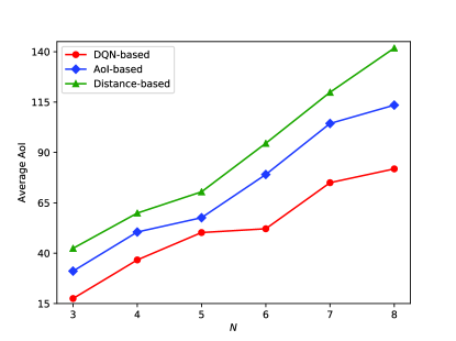
Fig.3 shows the average AoI with respect to the number of sensors for . We can easily observe that by adopting our DQN-based algorithm, the average AoI is smaller than that of the baseline algorithms. Moreover, the reduction of the average AoI is more significant for a larger . Fig. 3 also shows that the average AoI increases with the number of SNs. This is because, for a larger , the UAV has to fly farther to collect update packets. In addition, the SNs have to wait for a longer time to update their status, since the UAV can collect data packets from only one SN each time.
V Conclusions
In this paper, we have investigated the AoI-optimal data collection problem in UAV-assisted IoT networks, where a UAV collects status update packets and arrives at the final destination under both time and energy constraints. In order to minimize the wighted sum of the AoI, we have formulated the problem as a finite-horizon MDP. We have then designed a DRL-based data collection algorithm to find the optimal flight trajectory of the UAV and the transmission scheduling of the SNs. Moreover, we have conducted extensive simulations and shown that the DRL-based algorithm is superior to two baseline approaches, i.e., the AoI-based and the distance-based algorithms. Simulation results also demonstrated that the weighted sum of the AoI is monotonically decreasing with the SN’s coverage radius and monotonically increasing with the number of SNs.
References
- [1] M. Mozaffari, W. Saad, M. Bennis, Y.-H. Nam, and M. Debbah, “A Tutorial on UAVs for Wireless Networks: Applications, Challenges, and Open Problems,” http://arxiv.org/abs/1803.00680, Mar. 2018.
- [2] Y. Zeng and R. Zhang, “Energy-Efficient UAV Communication with Trajectory Optimization,” ArXiv160801828 Cs Math, Aug. 2016.
- [3] Y. Zeng, J. Xu, and R. Zhang, “Energy Minimization for Wireless Communication with Rotary-Wing UAV,” ArXiv180402238 Cs Math, Apr. 2018.
- [4] C. H. Liu, Z. Chen, J. Tang, J. Xu, and C. Piao, “Energy-Efficient UAV Control for Effective and Fair Communication Coverage: A Deep Reinforcement Learning Approach,” IEEE J. Sel. Areas Commun., vol. 36, no. 9, pp. 2059–2070, Sep. 2018.
- [5] J. Gong, T.-H. Chang, C. Shen, and X. Chen, “Flight Time Minimization of UAV for Data Collection over Wireless Sensor Networks,” ArXiv180102799 Cs Math, Jan. 2018.
- [6] U. Challita, W. Saad, and C. Bettstetter, “Deep Reinforcement Learning for Interference-Aware Path Planning of Cellular-Connected UAVs,” in 2018 IEEE International Conference on Communications (ICC), May 2018, pp. 1–7.
- [7] S. Kaul, R. Yates, and M. Gruteser, “Real-time status: How often should one update?” in Proc. IEEE INFOCOM, Orlando, FL, USA, Mar. 2012, pp. 2731–2735.
- [8] Y. Sun, E. Uysal-Biyikoglu, R. D. Yates, C. E. Koksal, and N. B. Shroff, “Update or Wait: How to Keep Your Data Fresh,” IEEE Trans. Inf. Theory, vol. 63, no. 11, pp. 7492–7508, Nov. 2017.
- [9] Z. Jiang, B. Krishnamachari, X. Zheng, S. Zhou, and Z. Niu, “Timely Status Update in Massive IoT Systems: Decentralized Scheduling for Wireless Uplinks,” ArXiv180103975 Cs Math, Jan. 2018.
- [10] M. A. Abd-Elmagid and H. S. Dhillon, “Average Peak Age-of-Information Minimization in UAV-assisted IoT Networks,” IEEE Trans. Veh. Technol., vol. 68, no. 2, pp. 2003–2008, 2019.
- [11] J. Liu, X. Wang, B. Bai, and H. Dai, “Age-optimal trajectory planning for UAV-assisted data collection,” in Proc. IEEE INFOCOM WKSHPS, Honolulu, HI, USA, Apr. 2018, pp. 553–558.
- [12] P. Tong, J. Liu, X. Wang, B. Bai, and H. Dai, “UAV-Enabled Age-Optimal Data Collection in Wireless Sensor Networks,” in Proc. IEEE ICC Workshops, Shanghai, CN, May 2019, pp. 1–6.
- [13] W. Li, L. Wang, and A. Fei, “Minimizing Packet Expiration Loss With Path Planning in UAV-Assisted Data Sensing,” IEEE Wirel. Commun. Lett., vol. 8, no. 6, pp. 1520–1523, Dec. 2019.
- [14] M. A. Abd-Elmagid, A. Ferdowsi, H. S. Dhillon, and W. Saad, “Deep Reinforcement Learning for Minimizing Age-of-Information in UAV-assisted Networks,” in Proc. IEEE Globecom, Puako, HI, USA, May 2019.
- [15] V. Mnih, K. Kavukcuoglu, D. Silver, A. A. Rusu, J. Veness, M. G. Bellemare, A. Graves, M. Riedmiller, A. K. Fidjeland, G. Ostrovski, S. Petersen, C. Beattie, A. Sadik, I. Antonoglou, H. King, D. Kumaran, D. Wierstra, S. Legg, and D. Hassabis, “Human-level control through deep reinforcement learning,” Nature, vol. 518, no. 7540, pp. 529–533, Feb. 2015.