Average Age of Changed Information in the Internet of Things

Abstract

The freshness of status updates is imperative in mission-critical Internet of things (IoT) applications. Recently, Age of Information (AoI) has been proposed to measure the freshness of updates at the receiver. However, AoI only characterizes the freshness over time, but ignores the freshness in the content. In this paper, we introduce a new performance metric, Age of Changed Information (AoCI), which captures both the passage of time and the change of information content. Also, we examine the AoCI in a time-slotted status update system, where a sensor samples the physical process and transmits the update packets with a cost. We formulate a Markov Decision Process (MDP) to find the optimal updating policy that minimizes the weighted sum of the AoCI and the update cost. Particularly, in a special case that the physical process is modeled by a two-state discrete time Markov chain with equal transition probability, we show that the optimal policy is of threshold type with respect to the AoCI and derive the closed-form of the threshold. Finally, simulations are conducted to exhibit the performance of the threshold policy and its superiority over the zero-wait baseline policy.

I Introduction

With the sharp proliferation of the Internet of Thing (IoT) devices and the rising need of mission-critical services, timely delivery of information has become increasingly important in real-time status update systems [1, 2]. The performance of such systems depends on the freshness of the status updates received by the destination [3, 4, 5]. Recently, the age of information (AoI) has been introduced to measure data freshness from the receiver’s perspective [6]. In particular, it is defined as the time elapsed since the generation of the most recent status update packet received by the destination. Essentially, AoI jointly characterizes the packet delay and the packet inter-generation time, which distinguishes AoI from conventional delay metrics. However, it ignores the content carried by the updates and the current knowledge of the receiver.

A natural question that arises then is whether it is sufficient to measure the freshness of updates via AoI only. There have been some recent efforts to answer this question. In [7], the mutual information between the state of the source and the received updates at the destination was defined as the freshness metric, which was proved to be a non-negative and non-increasing function of AoI if the sampling times are independent of the state of the source. For more general sampling patterns, the AoI is inadequate to reflect the freshness in information content and hence different metrics have been proposed in [8]-[10]. In [8], the authors proposed a metric, named sampling age, which is the time difference between the last ideal sampling time and the first actual sampling time. The sampling age is monotonically increasing with respect to estimation error for a Markov source, but the ideal sampling time is nontrivial to obtain. Age of synchronization (AoS) was proposed in [9] to measure the time that the process being tracked has changed. Particularly, AoS is defined as the time difference between the current time and the first update time after the previous synchronization time. Actually, it is implicitly assumed that the first update after each synchronization contains new information. The authors in [10] proposed age of incorrect information (AoII) as a new metric by combining time and estimation error penalty functions. As such, the AoII will increase with time when the receiver stays in an erroneous state. Note that an estimation error occurs when the current estimate at the receiver is different from the actual state of the process. Nonetheless, such an actual state cannot be perceived by the receiver unless the related update is delivered and hence, exactly depicting the AoII at the receiver between two successful transmissions is far from being trivial.

In this paper, we first introduce a new performance metric, referred to as age of changed information (AoCI), that characterizes the information freshness via both the passage of time and the change of information content. Then, we study the AoCI in a status update system consisting of a sensor and a destination. In particular, the sensor monitors the real-time status of a physical process, which is modeled by a two-state discrete time Markov chain, and transmits status update packets to the destination through a wireless channel, which incurs an update cost. We aim to find the optimal updating policy that minimizes the total average cost, which is the weighted sum of the AoCI and the update cost. By formulating this problem into a Markov decision process (MDP), we prove that the optimal updating policy is a threshold-type policy and further derive the threshold in closed-form with a special Markov chain model of the physical process. Simulation results show that the threshold policy can achieve lower total average cost than the zero-wait policy.

The rest of the paper is organized as follows: Section II presents the system model and introduces the proposed metric. In Section III, we provide the MDP formulation of the problem, analyze the switching structure of the optimal policy, and derive the threshold in closed-form. Simulation results are presented in Section IV, followed by the conclusion in Section V.

II System Overview

II-A System Model

We consider a time-slotted status update system which consists of a sensor and a destination (e.g., a monitor or an actuator). In each time slot, the sensor could remain idle to save energy. Or it could generate a status update about the underlying time-varying process (a.k.a. generate-at-will) and send it to the destination over an unreliable channel to refresh the destination. Let $a_{t}\in\{0,1\}$ be the action of the sensor in the $t$-th slot, where $a_{t}=1$ indicates that the sensor samples and transmits a new update, and $a_{t}=0$, otherwise. In general, there will be a cost associated with each update. We let $C_{u}$ denote the cost of an update. Moreover, the transmission time of each update is assumed to be equal to the duration of one time slot. Without loss of generality, the slot duration is normalized to unity.

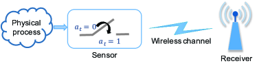
Figure 1: A model of a status update system.

Assume that the underlying time-varying physical process is modeled by a two-state discrete time Markov chain $\{X_{t};t\in\mathbb{N}\}$ with $X_{t}\in\{0,1\}$, where the duration of each state is equal to the slot length and the transition occurs just prior to the sampling decision at the beginning of each slot. The one-step state transition probability matrix is given by

$$\left[\begin{array}[]{cc}1-p_{c}&p_{c}\\ p_{c}&1-p_{c}\end{array}\right],$$ (1)

where $p_{c}\in(0,1)$ is the probability of changing states.

We assume that channel fading remains constant in each slot but independently changes over different slots. We also assume that the sensor transmits an update at a fixed rate and the channel state information is available only at the destination. As such, the transmission in each time slot may fail due to outage and the packet loss could be characterized by a memoryless Bernoulli process. Specifically, let $h_{t}\in\{0,1\}$ denote whether the transmission succeeds or fails, where $h_{t}=1$ indicates that the transmission is successful, and $h_{t}=0$, otherwise. We define the success probability as $\Pr\{h_{t}=1\}=p_{s}$ and the failure probability as $\Pr\{h_{t}=0\}=p_{f}=1-p_{s}$. Upon receiving the update packet, the destination feeds back a single-bit acknowledgement, which is assumed to be instant and error-free. If the transmission is failed and the sensor decides to transmit in the next slot, it would generate and transmit a new status update rather than retransmit the failed update. This is because, with the same success probability, retransmitting the failed out-of-date status update leads to a larger age.

II-B Freshness Metric

We assume that a status update is generated and transmitted at the beginning of a slot and it will be received by the end of the slot if the transmission succeeds. AoI, which is usually used to quantify the information freshness, is defined as the time elapsed since the generation of the latest status update received by the destination. Suppose that the update $i$ is generated and delivered at the time instants $g_{i}$ and $d_{i}$, respectively. Let $U(t)$ denote the time at which the latest status update successfully received by the destination was generated, i.e., $U(t)=\max\{g_{i}\mid d_{i}\leq t\}$. The AoI at the beginning of slot t is then given by

$$\delta_{t}=t-U(t).$$ (2)

Different from AoI, our proposed metric, AoCI, not only captures the time lag of the received update at the destination, but also incorporates the variation of the information content of the update. In particular, the AoCI decreases only when the content of the newly received update is different from the previous one, and increases otherwise. Let $n(t)=\max\{i|d_{i}\leq t\}$ be the index of the latest update received by the destination at the beginning of slot $t$ and $m(t)=\max\{j|Y_{j}\neq Y_{n(t)},d_{j}\leq d_{n(t)}\}$ be the index of the most recently update that has different content from the latest received update. $Y_{j}$ denotes the information content of update $j$, which is equal to the state of the physical process in the slot when update $j$ was generated. Then, we can define the AoCI at the beginning of slot $t$ as

$$\Delta_{t}=t-U^{\prime}(t),$$ (3)

where $U^{\prime}(t)=\min\{g_{k}|d_{m(t)}<d_{k}\leq d_{n(t)}\}$ represents the generation time of the next successfully received update packet after $m(t)$. It is worth noting that all the successfully received update packets after $m(t)$ has the same content with the latest received one.

Let $D_{t}\in\{0,1\}$ denote whether the content of a newly received update is different from that of the previously received one. If $D_{t}=1$, then the newly received update has different content. Otherwise, it has the same content. We define $p_{r}=\Pr(D_{t}=1)=\Pr(Y_{n(t)}=Y_{n(t)-1})$. Note that $Y_{n(t)}=X_{U(t)}$, we have $p_{r}=\Pr(X_{U(t)}=X_{U(t)-\delta})$, which is the return probability that a state of the physical process does not change after $\delta$ steps. According to (3), if a new status update generated by the sensor is successfully received by the destination (i.e., $a_{t}=1,h_{t}=1$) and it contains different content from the previously received update (i.e., $D_{t}=1$), then the AoCI decreases to one; otherwise, the AoCI increases by one. Then, the dynamics of the AoCI can be given by

$$\Delta_{t+1}=\begin{cases}1&a_{t}=1,h_{t}=1,D_{t}=1;\\ \Delta_{t}+1,&\text{otherwise}.\end{cases}$$ (4)

For ease of exposition, we use Fig. 2 to illustrate the evolution of AoCI over time.

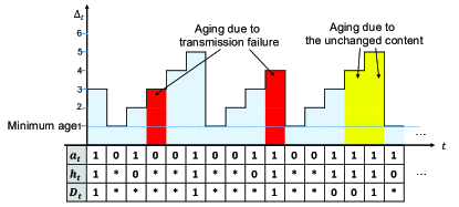
Figure 2: An illustration of the AoCI in a time-slotted status update system, where $*$ is used to represent the irrelevant values.

II-C Problem Formulation

The objective of this paper is to find an update policy $\pi=(a_{0},a_{1},\ldots)$ that minimizes the total average cost, which is the weighted sum of the AoCI and the update cost. By defining $\Pi$ as a set of stationary policies, our problem can be formulated as follows:

$$\min_{\pi\in\Pi}\limsup_{T\rightarrow\infty}\frac{1}{T}\stackrel{{\scriptstyle[}}{{t}}=0]{T}{\sum}\mathbb{E}[\Delta_{t}+\omega a_{t}C_{u}|s_{0}],$$ (5)

where $\omega$ is a weighting factor and is used to reflect the levels of importance and $s_{0}$ is the initial state.

III Updating Policy Design

III-A MDP Characterization

The optimization problem in (5) can be cast into an infinite horizon average cost Markov decision process $(\mathcal{S},\mathcal{A},\Pr(\cdot|\cdot,\cdot),C(\cdot,\cdot))$, where each item is explained as follows:

• States: The state of the MDP in time slot $t$ is defined to be the tuple of AoCI and AoI, i.e., $s_{t}\triangleq\left(\Delta_{t},\delta_{t}\right)$, which can take any value in $\mathbb{Z}^{+}\times\mathbb{Z}^{+}$. Therefore, the state space $\mathcal{S}$ is countable and infinite.

• Actions: The action in time slot $t$ is $a_{t}$ and the action set $\mathcal{A}=\{0,1\}$ is finite and countable.

• Transition Probability: Let $\Pr(s_{t+1}|s_{t},a_{t})$ denote the transition probability that state transits from $s_{t}$ to $s_{t+1}$ in the next slot by taking action $a_{t}$ in slot $t$. Since the failure of the packet transmission and the content change of the received updates are independent, according to the AoCI evolution dynamics (4), the transition probability can be written as

  $$\begin{cases}\Pr(s_{t+1}=(\Delta+1,\delta+1)|s_{t}=(\Delta,\delta),a_{t}=0)=1,\\ \Pr(s_{t+1}=(\Delta+1,\delta+1)|s_{t}=(\Delta,\delta),a_{t}=1)=p_{f},\\ \Pr(s_{t+1}=(\Delta+1,1)|s_{t}=(\Delta,\delta),a_{t}=1)=p_{s}p_{r}(\delta),\\ \Pr(s_{t+1}=(1,1)|s_{t}=(\Delta,\delta),a_{t}=1)=p_{s}(1-p_{r}(\delta)),\end{cases}$$ (6)

  and $\Pr(s_{t+1}|s_{t},a_{t})=0$ otherwise.

• Cost: Let $C(s_{t},a_{t})$ denote the instantaneous cost at state $s_{t}$ given action $a_{t}$, which is given by $C(s_{t},a_{t})=\Delta_{t}+\omega a_{t}C_{u}$.

The optimal policy $\pi^{*}$ to minimize the total average cost can be obtained by solving the following Bellman equation [11]:

$$\theta+V(s)=\min_{a\in\{0,1\}}\left\{C(s,a)+\sum_{s^{\prime}\in\mathcal{S}}\Pr(s^{\prime}|s,a)V(s^{\prime})\right\},\forall s\in\mathcal{S},$$ (7)

where $\theta$ is the optimal value to (5) and $V(s)$ is the value function which is a mapping from $s$ to real values. Moreover, for any $s\in\mathcal{S}$, the optimal policy can be given by

$$\pi^{*}(s)=\arg\min_{a\in\{0,1\}}\left\{C(s,a)+\sum_{s^{\prime}\in\mathcal{S}}\Pr(s^{\prime}|s,a)V(s^{\prime})\right\}.$$ (8)

It can be seen from (8) that the optimal policy $\pi^{*}$ depends on the value function $V(\cdot)$, for which there is no closed-form solution in general [11]. In the literature, various numerical algorithms, such as value iteration and policy iteration, have therefore been proposed. However, these methods are usually computationally demanding due to the curse of dimensionality and few insights for the optimal policy can be leveraged. Therefore, we study the structural properties of the optimal updating policy in the sequel.

III-B Structural Analysis and Optimal Policy

We consider a special case that $p_{c}=1/2$. In this case, the return probability $p_{r}(\delta)=1/2$ for all $\delta$. In other word, $p_{r}$ is irrespective of $\delta$. Hence, we can simplify the states of the MDP. In particular, the state in slot $t$ reduces to the AoCI, i.e., $s_{t}=\Delta_{t}$, and the state transition probability in (6) can be simplified as

$$\begin{cases}\Pr(s_{t+1}=\Delta+1|s_{t}=\Delta,a_{t}=0)=1,\\ \Pr(s_{t+1}=\Delta+1|s_{t}=\Delta,a_{t}=1)=p_{f}+p_{s}p_{r},\\ \Pr(s_{t+1}=1|s_{t}=\Delta,a_{t}=1)=p_{s}(1-p_{r}),\end{cases}$$ (9)

and $\Pr(s_{t+1}|s_{t},a_{t})=0$ otherwise. Based on the simplified state space and transition probability, we present the monotonicity property of $V(s)$ in the following lemma.

Lemma 1.

The value function V(s) is a non-decreasing function for $s\in\mathcal{S}$.

Proof:

See Appendix -A. ∎

Then, we provide results on the structure of the optimal updating policy in the following theorem.

Theorem 2.

For $s\in\mathcal{S}$, the optimal policy has a switching structure, that is if $\pi^{*}(s_{1})=1$, then $\pi^{*}(s_{2})=1$ for all $s_{2}\geq s_{1}$.

Proof:

See Appendix -B. ∎

According to Theorem 2, the optimal policy can be represented as a threshold policy, which is given by

$$\pi^{*}(s)=\begin{cases}1,&\text{if }s\geq\Omega^{*},\\ 0,&\text{otherwise},\end{cases}$$ (10)

where $\Omega^{*}$ is the threshold at which the switching occurs. Thanks to the simplifications in the special case, we are able to derive the closed-form of $\Omega^{*}$.

Theorem 3.

The optimal threshold $\Omega^{*}$ of the threshold policy is given by

$$\Omega^{*}=\frac{\sqrt{p_{z}+2\omega C_{u}(1-p_{z})}-p_{z}}{1-p_{z}},$$ (11)

where $p_{z}=p_{f}+p_{s}p_{r}$.

Proof:

See Appendix -C. ∎

If $\Omega^{*}$ is an integer, the optimal policy is shown in (10). Otherwise, the optimal policy is given by

$$\pi^{*}(s)=\begin{cases}1,&\text{if }s\geq\left\lceil\Omega^{*}\right\rceil,\\ {\bf 1}_{(x\leq\mu)},&\text{if }s=\left\lfloor\Omega^{*}\right\rfloor,\\ 0,&\text{if }s<\left\lfloor\Omega^{*}\right\rfloor,\end{cases}$$ (12)

where $\bm{1}_{(\cdot)}$ is an indicator function, $x\in[0,1]$ is a uniform random variable, and $\mu=\frac{\left\lceil\Omega^{*}\right\rceil-\Omega^{*}}{\left\lceil\Omega^{*}\right\rceil-\left\lfloor\Omega^{*}\right\rfloor}$. Specifically, $\pi^{*}(\left\lfloor\Omega^{*}\right\rfloor)=1$ with probability $\mu$ and $\pi^{*}(\left\lfloor\Omega^{*}\right\rfloor)=0$ with probability $1-\mu$.

IV Simulation Results

In this section, we present the simulation results of the optimal updating policy to investigate the effects of system parameters and compare the optimal updating policy with zero-wait policy.

Fig. 3 shows the optimal threshold of the optimal updating policy with respect to $p_{s}$ for different $C_{u}$. It can be seen that the larger the cost, the larger the threshold is. This is evident from Theorem 3. We can observe that the smaller the $p_{s}$, the larger the threshold is. This is because, when $p_{s}$ is small, the sensor has to sample and transmit multiple times until the destination successfully receives an update packet. Therefore, it is efficient to update the status only when the AoCI is large.

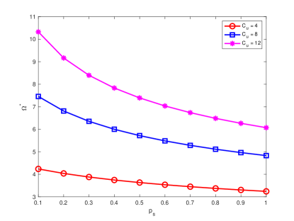
Figure 3: The optimal threshold for different values of $p_{s}$ ($p_{c}=0.5$ and $\omega=1$).

Fig. 4 illustrates the total average cost of the optimal policy with respect to $p_{s}$ for different $C_{u}$. The effect of $p_{s}$ on the performance can be seen immediately: the larger the $p_{s}$, the smaller the total average cost is. As $p_{s}$ increases, the transmission of an update is much easier to be successful, and hence the average AoCI and the average update cost are both reduced. Moreover, larger $C_{u}$ results in an increase in the total average cost as expected, and the gap between the total average cost for different $C_{u}$ values is almost constant with respect to $p_{s}$.

Figure 4: Effect of $p_{s}$ on the total average cost for different values of $C_{u}$ ($p_{c}=0.5$ and $\omega=1$).

In Fig. 5, we compare the total average cost of the optimal policy and the zero-wait baseline policy. In the zero-wait policy, the sensor samples and transmits the status update in each time slot. We can see that the optimal policy is superior to the zero-wait policy and the reduction of the total average cost increases with increasing $p_{s}$. This is due to the fact, as shown in Fig. 6, that the zero-wait policy achieves a smaller AoCI but suffers from a constant update cost, while the optimal policy can strike a balance between the AoCI and the update cost. In particular, compared with the zero-wait policy, the optimal policy has a larger AoCI because the sensor remains idle until the AoCI is larger than a threshold. However, its update cost decreases as $p_{s}$ grows and hence the optimal policy is more cost-efficient.

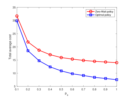
Figure 5: Comparison between the optimal policy and zero-wait policy in terms of the total average cost ($p_{c}=0.5$, $C_{u}=12$ and $\omega=1$).

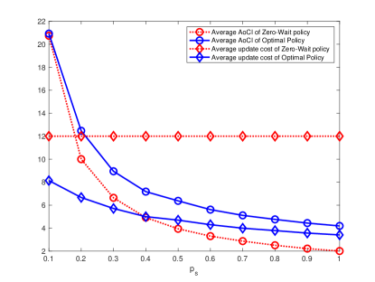
Figure 6: Comparison between the optimal policy and zero-wait policy in terms of the average AoCI and the average update cost ($p_{c}=0.5$, $C_{u}=12$ and $\omega=1$).

V Conclusion

In this paper, we have proposed a new freshness metric that addresses the ignorance of information content in the conventional AoI. Named as the age of changed information, this new metric not only measures the freshness by the passage of time but also captures the information content of the updates at the destination. We have studied the updating policy in the status update system by taking both the AoCI and the update cost into consideration and formulated the updating problem as an infinite horizon average cost MDP. We have shown that the optimal updating policy in a special case is of threshold type, which reveals an intrinsic tradeoff between the average AoCI and the update cost. Simulation results have shown the effects of the unreliable channel on the total average cost. Through the comparison between the threshold policy and the zero-wait policy, the threshold policy is shown to yield significant performance gain in terms of the total average cost compared to a zero-wait policy. Future work will address some extensions such as modeling the physical process with a more general Markov chain model and incorporating time-correlated channel statistics.

-A Proof of Lemma 1

Based on the value iteration algorithm (VIA) [11], we use mathematical induction to prove Lemma 1. For each state $s$, let $V_{k}(s)$ be the value function at iteration $k$. In VIA, the value function can be updated as follows:

$$V_{k+1}(s)=\min_{a}\left\{C(s,a)+\sum_{s^{\prime}\in\mathcal{S}}\Pr(s^{\prime}|s,a)V_{k}(s^{\prime})\right\},\forall s\in\mathcal{S}.$$ (13)

Under any initialization of the initial value $V_{0}(s)$, the sequence $\{V_{k}(s)\}$ converges to the value function in the Bellman equation (7) [11], i.e.,

$$\lim_{k\rightarrow\infty}V_{k}(s)=V(s),\forall s\in\mathcal{S}.$$ (14)

Therefore, the monotonicity of $V(s)$ in $\mathcal{S}$ can be guaranteed by proving that for any $s_{1},s_{2}\in\mathcal{S}$, such that $s_{1}\leq s_{2}$,

$$V_{k}(s_{1})\leq V_{k}(s_{2}),\quad k=0,1,\ldots$$ (15)

Then, we prove (15) via mathematical induction. Without loss of generality, we initialize $V_{0}(s)=0$ for all $s\in\mathcal{S}$. Thus, (15) holds for $k=0$. Next, we assume that (15) holds up till $k>0$ and we examine whether it holds for $k+1$. Let $Q_{k}(s,a)$ denote the state-action value function at iteration $k$, which is defined as

$$Q_{k}(s,a)=C(s,a)+\sum_{s^{\prime}\in\mathcal{S}}\Pr(s^{\prime}|s,a)V_{k}(s^{\prime}),$$ (16)

for all $s\in\mathcal{S}$ and $a\in\mathcal{A}$. Then, the value function at iteration $k+1$ can be represented as

$$V_{k+1}(s)=\min\limits_{a\in\{0,1\}}Q_{k}(s,a).$$ (17)

When $a=0$, we have $Q_{k}(s_{1},0)=s_{1}+\mathop{V_{k}(s_{1}+1)}$ and $Q_{k}(s_{2},0)=s_{2}+\mathop{V_{k}(s_{2}+1)}$. Since $s_{1}\leq s_{2}$ and $V_{k}(s_{1})\leq V_{k}(s_{2})$, we can easily see that $Q_{k}(s_{1},0)\leq Q_{k}(s_{2},0)$.

When $a=1$, we have

$$Q_{k}(s_{1},1)= s_{1}+\omega C_{u}$$

$$+(p_{f}+p_{s}p_{r})\mathop{V_{k}(s_{1}+1)}+p_{s}(1-p_{r})V_{k}(1)$$

and

$$Q_{k}(s_{2},1)= s_{2}+\omega C_{u}$$

$$+(p_{f}+p_{s}p_{r})\mathop{V_{k}(s_{2}+1)}+p_{s}(1-p_{r})V_{k}(1).$$

Bearing in mind that $V_{k}(s_{1})\leq V_{k}(s_{2})$, we can also verify that $Q_{k}(s_{1},1)\leq Q_{k}(s_{2},1)$.

Altogether, we can assert that $V_{k+1}(s_{1})\leq V_{k+1}(s_{2})$ for any $k$. By taking limits on both sides of (15) and by (14), we complete the proof of Lemma 1.

-B Proof of Theorem 2

Let $Q(s,a)$ denote the state-action value function, i.e.,

$$Q(s,a)=s+\omega aC_{u}+\mathop{\sum_{s^{\prime}\in\mathcal{S}}\Pr(s^{\prime}|s,a)V(s^{\prime})}.$$ (18)

The optimal policy can be expressed as

$$\pi^{*}(s)=\arg\min\limits_{a\in\{0,1\}}Q(s,a).$$ (19)

Suppose $\pi^{*}(s_{1})=1$, we have $Q(s_{1},0)-Q(s_{1},1)\geq 0$. Therefore, the optimal updating policy has a switching structure if $Q(s,a)$ has a sub-modular structure, that is,

$$Q(s_{1},0)-Q(s_{1},1)\leq Q(s_{2},0)-Q(s_{2},1),$$ (20)

for any $s_{1},s_{2}\in\mathcal{S}$ and $s_{1}\leq s_{2}$.

According to the definition of $Q(s,a)$, we have

$$Q(s_{1},0)-Q(s_{1},1)$$

$$= p_{s}(1-p_{r})(V(s_{1}+1)-V(1))-\omega C_{u}$$

and

$$Q(s_{2},0)-Q(s_{2},1)$$

$$= p_{s}(1-p_{r})(V(s_{2}+1)-V(1))-\omega C_{u}.$$

Since $V\left(s_{1}+1\right)\leq V(s_{2}+1)$, it is easy to see that (20) holds. Along with $Q(s_{1},0)-Q(s_{1},1)\geq 0$, we complete the proof of Theorem 2.

-C Proof of Theorem3

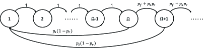
Figure 7: The states transitions under a threshold policy.

For any threshold policy with the threshold of $\Omega$, the MDP can be modeled through a Discrete Time Markov Chain (DTMC) with the same states, which is illustrated in Fig. 7. Let $\varphi_{s}$ denote the steady state probability of state $s$. According to Fig. 7, we have

$$\varphi_{s}=\begin{cases}\varphi_{1},&\text{if }s\leq\Omega,\\ \varphi_{1}p_{z}^{s-\Omega},&\text{otherwise},\end{cases}$$ (21)

where $p_{z}=p_{f}+p_{s}p_{r}$. Along with $\stackrel{{\scriptstyle[}}{{i}}=1]{\infty}{\sum}\varphi_{i}=1$, we can derive $\varphi_{s}$ in closed-form as follows:

$$\varphi_{s}=\begin{cases}\frac{1-p_{z}}{\Omega(1-p_{z})+p_{z}},&\text{if }s\leq\Omega,\\ \frac{(1-p_{z})p_{z}^{s-\Omega}}{\Omega(1-p_{z})+p_{z}},&\text{otherwise}.\end{cases}$$ (22)

Then, the expected cost under the threshold policy can be computed as:

$$J_{\Omega} =\stackrel{{\scriptstyle[}}{{s}}=1]{\infty}{\sum}\varphi_{s}(s+\omega C_{u}{\bf 1}_{(s\geq\Omega)})$$

$$=\sum_{s=1}^{\Omega-1}\varphi_{s}s+\sum_{s=\Omega}^{\infty}\varphi_{s}(s+\omega C_{u})$$

$$=\frac{1-p_{z}}{\Omega(1-p_{z})+p_{z}}\left(\frac{\Omega^{2}-\Omega}{2}+\frac{\Omega+\omega C_{u}}{1-p_{z}}+\frac{p_{z}}{(1-p_{z})^{2}}\right).$$ (23)

Since $J_{\Omega}$ is a convex function of $\Omega$ by (23), the optimal threshold can be obtained by setting the derivative $\partial J_{\Omega}/\partial\Omega$ to zero. Specifically,

$$\Omega^{*}=\frac{\sqrt{p_{z}+2\omega C_{u}(1-p_{z})}-p_{z}}{1-p_{z}},$$ (24)

which concludes our proof.

References

- [1] M. R. Palattella, M. Dohler, A. Grieco, G. Rizzo, J. Torsner, T. Engel, and L. Ladid, “Internet of Things in the 5G Era: Enablers, Architecture, and Business Models,” IEEE J. Sel. Areas Commun., vol. 34, no. 3, pp. 510–527, Mar. 2016.
- [2] P. Schulz, M. Matthe, H. Klessig, M. Simsek, G. Fettweis, J. Ansari, S. A. Ashraf, B. Almeroth, J. Voigt, I. Riedel, A. Puschmann, A. Mitschele-Thiel, M. Muller, T. Elste, and M. Windisch, “Latency Critical IoT Applications in 5G: Perspective on the Design of Radio Interface and Network Architecture,” IEEE Commun. Mag., vol. 55, no. 2, pp. 70–78, Feb. 2017.
- [3] J. Liu, X. Wang, B. Bai, and H. Dai, “Age-optimal trajectory planning for UAV-assisted data collection,” in Proc. IEEE INFOCOM WKSHPS, Honolulu, HI, USA, Apr. 2018, pp. 553–558.
- [4] P. Tong, J. Liu, X. Wang, B. Bai, and H. Dai, “UAV-Enabled Age-Optimal Data Collection in Wireless Sensor Networks,” in Proc. IEEE ICC Workshops, Shanghai, CN, May 2019, pp. 1–6.
- [5] C. Xu, H. H. Yang, X. Wang, and T. Q. S. Quek, “Optimizing Information Freshness in Computing enabled IoT Networks,” IEEE Internet Things J., pp. 1–1, 2019.
- [6] S. Kaul, R. Yates, and M. Gruteser, “Real-time status: How often should one update?” in Proc. IEEE INFOCOM, Orlando, FL, USA, Mar. 2012, pp. 2731–2735.
- [7] Y. Sun and B. Cyr, “Sampling for Data Freshness Optimization: Non-linear Age Functions,” http://arxiv.org/abs/1812.07241, Dec. 2018.
- [8] C. Kam, S. Kompella, G. D. Nguyen, J. E. Wieselthier, and A. Ephremides, “Towards an effective age of information: Remote estimation of a Markov source,” in IEEE INFOCOM WKSHPS, Honolulu, HI, USA, Apr. 2018, pp. 367–372.
- [9] J. Zhong, R. D. Yates, and E. Soljanin, “Two Freshness Metrics for Local Cache Refresh,” in Proc. IEEE ISIT, Vail, CO, Jun. 2018, pp. 1924–1928.
- [10] A. Maatouk, S. Kriouile, M. Assaad, and A. Ephremides, “The Age of Incorrect Information: A New Performance Metric for Status Updates,” http://arxiv.org/abs/1907.06604, Jul. 2019.
- [11] Dimitri P. Bertsekas, Dynamic Programming and Optimal Control-II, 3rd ed. Athena Scientific, 2007, vol. II.