A Globally Convergent Newton Method for Polynomials

Abstract

Newton’s method for polynomial root finding is one of mathematics’ most well-known algorithms. The method also has its shortcomings: it is undefined at critical points, it could exhibit chaotic behavior and is only guaranteed to converge locally. Based on the Geometric Modulus Principle for a complex polynomial $p(z)$, together with a Modulus Reduction Theorem proved here, we develop the Robust Newton’s method (RNM), defined everywhere with a step-size that guarantees an a priori reduction in polynomial modulus in each iteration. Furthermore, we prove RNM iterates converge globally, either to a root or a critical point. Specifically, given $\varepsilon$ and any seed $z_{0}$, in $t=O(1/\varepsilon^{2})$ iterations of RNM, independent of degree of $p(z)$, either $|p(z_{t})|\leq\varepsilon$ or $|p(z_{t})p^{\prime}(z_{t})|\leq\varepsilon$. By adjusting the iterates at near-critical points, we describe a modified RNM that necessarily convergence to a root. In combination with Smale’s point estimation, RNM results in a globally convergent Newton’s method having a locally quadratic rate. We present sample polynomiographs that demonstrate how in contrast with Newton’s method RNM smooths out the fractal boundaries of basins of attraction of roots. RNM also finds potentials in computing all roots of arbitrary degree polynomials. A particular consequence of RNM is a simple algorithm for solving cubic equations.

Keywords: Complex Polynomial, Newton Method, Taylor Theorem.

1 Introduction

One of mathematics’ most well-known algorithms, the Newton’s method for polynomial root finding stands out as prolific and multi-faceted. Fruitful enough to remain of continual research interest, it is nevertheless simple enough to be a perennial topic of high school calculus courses; combined with computer graphics tools it can yield dazzling fractal images, infinitely complex by near-definition.

The development of iterative techniques such as Newton’s method complement those of algebraic techniques for solving a polynomial equation, one of the most fundamental and influential problems of science and mathematics. Through historic and profound discoveries we have come to learn that beyond quartic polynomials there is no general closed formula in radicals for the roots. The book of Irving [7] is dedicated to the rich history in the study and development of formulas for quadratic, cubic, quadratic and quintic polynomials. This complementary relationship between algebraic and iterative techniques becomes evident even for approximating such mundane numbers as the square-root of two, demonstrating the fact that for computing purposes, we must resort to iterative algorithms. These in turn have resulted in new applications and directions of research.

Although Newton’s method is traditionally used to find roots of polynomials with real-valued coefficients, it is also valid for complex polynomials, i.e., polynomials of the form

$$p(z)=a_{n}z^{n}+\cdots+a_{1}z+a_{0},$$ (1)

with coefficients $a_{j}\in\mathbb{C}$, $z=x+iy$, $i=\sqrt{-1}$, and $x,y\in\mathbb{R}$. The Newton iterations are defined recursively by the formula

$$z_{j+1}=z_{j}-\frac{p(z_{j})}{p^{\prime}(z_{j})},\quad j=0,1,...,$$ (2)

where $z_{0}\in\mathbb{C}$ is the starting point, or seed, and $p^{\prime}(z)$ is the derivative of $p(z)$. As in the case of real polynomials, the derivative function $p^{\prime}(z)$ is the limit of difference quotient $(p(z+\delta z)-p(z))/\delta z$ as $\delta z$ approaches zero and can easily be shown to be the following polynomial, the complex analog of the real case

$$p^{\prime}(z)=na_{n}z^{n-1}+(n-1)a_{n-1}z^{n-2}+\dots+2a_{2}z+a_{1}.$$ (3)

We can thus view $z_{j+1}$, called the Newton iterate, as an adjustment of the current iterate, $z_{j}$, in the direction of $-p(z_{j})/p^{\prime}(z_{j})$, called Newton direction. The sequence $\{z_{j}\}_{j=0}^{\infty}$ is called the orbit of $z_{0}$, denoted by $O^{+}(z_{0})$. The basin of attraction of a root $\theta$ of $p(z)$ is the set of all seeds $z_{0}$ whose orbit converges to $\theta$, denoted by $\mathcal{A}(\theta)$. It can be shown that $\mathcal{A}(\theta)$ is an open set, i.e. if $c\in\mathcal{A}(\theta)$, an open disc centered at $c$ is also contained in $\mathcal{A}(\theta)$. For example, for $p(z)=z^{2}-1$, the basin of attraction $\theta=1$, as proved by Cayley [4], is the half-plane consisting of the set of all $z=x+iy$ with $x>0$. However, in the case of $p(z)=z^{3}-1$, the basin of attraction of $\theta=1$ consists of the union of countably infinite disjoint open connected sets, only one of which contains $\theta$, called the immediate basin of attraction of $\theta$, see Figure 1. A set is connected if for any pair of points in the set there is a path connecting the points, the path contained in the set. Beyond quadratic polynomials, the boundary of the basin of attraction of a root is fractal with the peculiar property that it is also the boundary of any other root. Newton iterations can be viewed as fixed point iterations with respect to the rational function $N_{p}(z)=z-p(z)/p^{\prime}(z)$. Notably, the iterate $z_{j+1}$ is undefined if $z_{j}$ is a critical point of $p(z)$, i.e., if $p^{\prime}(z_{j})=0$. When the iterate $z_{j+1}$ is well-defined, it can be interpreted as the root of the linear approximation to $p(z)$ at $z_{j}$.

It is natural to ask if the orbit of a point with respect to Newton iterations converge to a root. More specifically, given $\varepsilon>0$ and a seed $z_{0}$, can we decide if the corresponding orbit results in a point $z_{j}$ such that $|p(z_{j})|<\varepsilon$? Blum et al. [3] consider such question and prove that even for a cubic polynomial it is undecidable. Their notion of decidability in turn requires a notion of machines defined over the real numbers. In a different study Hubbard et al. [6] show all roots of a polynomial can be computed solely via Newton’s method when iterated at certain finite set of points. In summary, in this article we develop a modified Newton’s method, where starting at any seed the corresponding orbit is guaranteed to converge to a root.

To discuss convergence of our method we must consider modulus of a complex number $z=x+iy$, defined as $|z|=\sqrt{x^{2}+y^{2}}$. Equivalently, $|z|=\sqrt{z\overline{z}}$, where $\overline{z}=x-iy$ is the conjugate of $z$. In general, Newton iterates do not necessarily monotonically decrease the modulus of the polynomial after each iteration, i.e., at an arbitrary step $j$, we may obtain $p(z_{j+1})$ such that $|p(z_{j+1})|>|p(z_{j})|$. For example, if $p(z)=z^{2}-1$, then $|p(z_{j+1})|>>|p(z_{j})|$ for small $|z_{j}|$. However, for a general polynomial, near a simple root $\theta$ (i.e. $p^{\prime}(\theta)\not=0$), the rate of convergence is known to be quadratic, i.e., $|z_{j+1}-\theta|\approx|z_{j}-\theta|^{2}$. Thus once a point is in the region of quadratic convergence of a root, in very few subsequent iterations we obtain highly accurate approximation to the root. Another drawback in Newton’s method is that its orbits may not even converge; some cycle. For instance, in the case of $p(z)=z^{3}-2z+2$, the Newton iterate at $z_{0}=0$ is $z_{1}=1$ and the iterate at $z_{1}$ is $z_{0}$, resulting in a cycle between $0$ and $1$. In fact under Newton iterations a neighborhood of $0$ gets mapped to a neighborhoods of $1$ and conversely. Figure 1 shows the corresponding polynomiograph. A seed selected in the white area will not converge to any of the roots. Finally, an orbit may converge yet be complex to the point of practical unwieldiness, even when $p(z)$ is a cubic polynomial.

Historically, Cayley [4] is among the pioneers who considered Newton iterations for a complex polynomial $p(z)$ and proved that the basin of attraction of each root of $p(z)=z^{2}-1$ equals that root’s Voronoi region, the set of all points closer to that root than to the other. Points on the $y$-axis do not converge. One may anticipate that analogous Voronoi region property would hold with respect to the three roots of $z^{3}-1$. However, this is not so as the well-known fractal image of it shows (see e.g. [17] and other sources such as [10]). Figure 1 is a depiction of this. The study of the global dynamics of Newton’s method is a fascinating and deep subject closely related to the study of rational iteration functions, see e.g. [1] and [10]. Smale’s one-point theory, [19], is an outstanding result that ensures quadratic rate of convergence to a root, provided a certain computable condition is satisfied at a seed ( see (45)). However, it is only a local result.

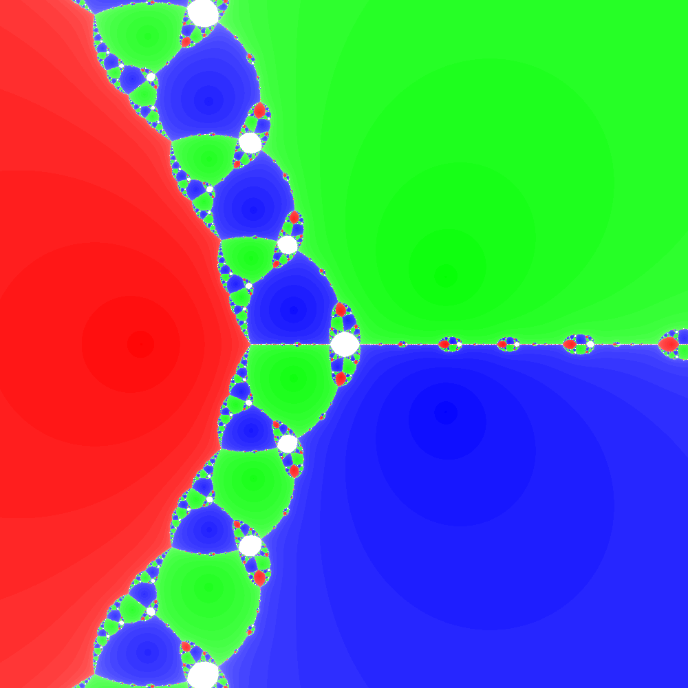
Figure 1: Polynomiograph of Newton’s method for $z^{3}-1$ (left) and $z^{3}-2z+2$.

In this article we develop a robust version of Newton’s method based on the minimization of the modulus of a complex polynomial $p(z)$ and a fresh look at the problem. The algorithm is easy to implement so that the interested reader familiar with complex numbers and Horner’s method can implement it and test its performance, or generate computer graphics based on the iterations of points in a square region and color coding analogous to methods for generation of fractal images.

To consider modulus minimization, it is more convenient to consider square of the modulus, namely the function

$$F(z)=|p(z)|^{2}=p(z)\overline{p(z)}.$$ (4)

Clearly, $\theta$ is a root of $p(z)$ if and only if $F(\theta)=0$. Indeed several proofs of the Fundamental Theorem of Algebra (FTA) rely on the minimization of $F(z)$. To prove the FTA it suffices to show that the minimum of $F(z)$ over $\mathbb{C}$ is attained at a point $z_{*}$ and $F(z_{*})=0$. The proof that the minimum is attained is shown by first observing that $|p(z)|$ approaches infinity as $|z|$ approaches infinity. Thus the set $S=\{z:|p(z)|\leq|p(0)|\}$ is bounded. Then, by continuity of $|p(z)|$ it follows that $S$ is also closed, hence compact. Thus, the minimum of $F(z)$ over $S$ is attained and coincides with its minimum over $\mathbb{C}$. Now to prove $F(z_{*})=0$, one assumes otherwise and derives a contradiction. To derive a contradiction, it suffices to exhibit a direction of descent for $F(z)$ at $z_{*}$, i.e. a point $u\in\mathbb{C}$ and a positive real number $\alpha_{*}$ such that

$$F(z_{*}+\alpha u)<F(z_{*}),\quad\forall\alpha\in(0,\alpha_{*}).$$ (5)

For proofs of the FTA based on a descent direction, see [5, 11, 13, 14, 15]. In fact, [11] describes the Geometric Modulus Principle (GMP), giving a complete characterization of all descent and ascent directions for $F(z)$ at an arbitrary point $z_{0}$:

If $z_{0}$ is not a root of $p(z)$ the ascent and descent directions at $z_{0}$ evenly split into alternating sectors of angle $\pi/2k$, where $k$ is the smallest index for which $p^{(k)}(z_{0})\not=0$. Specifically, if $\overline{p(z_{0})}p^{(k)}(z_{0})=r_{0}e^{{i}\alpha}$ then $e^{i\theta}$ is an ascent direction if $\theta$ satisfies the following

$$\frac{2N\pi-\alpha}{k}-\frac{\pi}{2k}<\theta<\frac{2N\pi-\alpha}{k}+\frac{\pi}{2k},\quad N\in\mathbb{Z}.$$ (6)

The remaining are sectors of descent. Figure 2 shows this property for $k=1,2,3$.

Figure 2: Sectors of ascent (gray) and descent (white) for $k=1,2,3$.

In [12] a specific descent direction is given, resulting in a short proof of the FTA. However, neither [11] nor [12] provide a guaranteed step-size (see $\alpha_{*}$ in (5)) and consequently no estimate of the decrement $F(z_{*}+\alpha_{*}u)-F(z_{*})$. We accomplish these in this article.

By making use of GMP for a complex polynomial $p(z)$, together with a Modulus Reduction Theorem proved in the article, we develop the Robust Newton Method (RNM), defined everywhere with a guaranteed amount of reduction in the polynomial modulus in the next iteration. Furthermore, we prove the iterates converge globally, either to a root or a critical point. Specifically, given $\varepsilon$, for any seed $z_{0}$, in $t=O(1/\varepsilon^{2})$ iterations of RNM, either $|p(z_{t})|\leq\varepsilon$ or $|p(z_{t})p^{\prime}(z_{t})|\leq\varepsilon$. By adjusting RNM iterates at near-critical points, the iterates of a modified RNM bypass critical points and converge to a root. In combination with Smale’s condition, RNM results in a globally convergent method, having locally quadratic rate of convergence. We present small degree polynomiographs for RNM and discuss its potentials in computing all roots of an arbitrary degree polynomial. In particular, RNM gives a simple algorithm for solving cubic equations.

The article is organized as follows. In Section 2, we describe the necessary ingredients and define the Robust Newton iterate. Then we state the modulus reduction theorem (Theorem 1), describe the Robust Newton Method (RNM), state the complexity theorem for RNM (Theorem 2), and state the modified RNM, as well as its convergence properties (Theorem 3). All proofs are given in subsequent sections. Thus an interested reader can begin implementing the algorithm after reading Section 2. To make the results clear for the reader, in Section 3 we consider solving quadratic and cubic equations via RNM, prove convergence properties for quadratics (Theorem 4) and then for cubics (Theorem 5). In Section 4, we prove Theorem 1 but first we state and prove two auxiliary lemmas. In Section 5, we make use of Theorem 1 to prove Theorem 2 and subsequently we prove the convergence of modified RNM, Theorem 3. In Section 6, we consider further algorithmic application of RNM, in particular its combination with Smale’s one point theory, as well as potentials of RNM in computing all roots of a polynomial. We end with concluding remarks.

2 The Robust Newton Iterate

In this section we describe how to compute a direction of descent and step-size for $F(z)=|p(z)|^{2}$ at any seed $z_{0}$ in order to get a new point $z_{1}$ and state an estimate of the decrement, $F(z_{1})-F(z_{0})$. This direction is a special direction selected in a sector of descent as depicted in Figure 2. When $k>1$ there are $2k$ such sectors, however it suffices to choose only one such sector.

Given $z\in\mathbb{C}$ with $p(z)\not=0$, set

$$k\equiv k(z)=\min\{j\geq 1:p^{(j)}(z)\neq 0\},\quad A(z)=\max\bigg{\{}\frac{|p^{(j)}(z)|}{j!}:j=0,\dots,n\bigg{\}},$$ (7)

$$u_{k}\equiv u_{k}(z)=\frac{1}{k!}p(z){\overline{p^{(k)}(z)}},\quad\gamma=\phantom{-}2\cdot Re(u_{k}^{k-1}),\quad\delta=-2\cdot Im(u_{k}^{k-1}),\quad c_{k}=\max\{|\gamma|,|\delta|\}.$$ (8)

Finally, let $\theta$ be any angle that satisfies the following conditions.

$$\theta=\begin{cases}0,&{~{}\rm if~{}}c_{k}=|\gamma|,\gamma<0\\ \pi/k,&{~{}\rm if~{}}c_{k}=|\gamma|,\gamma>0\\ \pi/2k,&{~{}\rm if~{}}c_{k}=|\delta|,\delta<0\\ 3\pi/2k,&{~{}\rm if~{}}c_{k}=|\delta|,\delta>0\\ \end{cases}.$$ (9)

Definition 1.

The Robust Newton iterate at $z$ is defined as

$$\widehat{N}_{p}(z)=z+\frac{C_{k}}{3}\frac{u_{k}}{|u_{k}|}e^{i\theta},\quad C_{k}=\frac{c_{k}|u_{k}|^{2-k}}{6A^{2}(z)}.$$ (10)

The Robust Newton Method (RNM) is defined according to the iteration:

$$z\leftarrow\widehat{N}_{p}(z).$$ (11)

The RNM orbit of $z$ is denoted by $\widehat{O}^{+}(z)$. We refer to $(u_{k}/|u_{k}|)e^{i\theta}$ as the Normalized Robust Newton direction at $z$. We call $C_{k}/3$ the step-size. In particular, when $k=1$, $c_{1}=2$ and $\theta=\pi$. Thus $e^{i\theta}=e^{i\pi}=-1$, and $C_{1}=|u_{1}|/3A^{2}(z)$ so that

$$\widehat{N}_{p}(z)=z-\frac{p(z)\overline{p^{\prime}(z)}}{9A^{2}(z)}=z-\frac{|p^{\prime}(z)|^{2}}{9A^{2}(z)}\frac{p(z)}{p^{\prime}(z)}.$$ (12)

Remark 1.

According to Definition 1 the Robust Newton iterate is defined everywhere, including at critical points. In particular, when $k=1$ RNM Direction is simply a positive scalar multiple of the standard Newton direction. Also, by the definition of $A(z)$, ${|p^{\prime}(z)|^{2}}/{9A^{2}(z)}\leq 1/9$. Thus the Robust Newton iterate always lies on the line segment between $z$ and the standard Newton iterate, $z-p(z)/p^{\prime}(z)$. This seemingly simple modification when $k=1$, together with the ability to define the iterates when $k>1$, will guarantee that the polynomial modulus at the new point, $\widehat{N}_{p}(z)$, will necessarily decrease by a computable estimate as described by the main theorem, Theorem 1:

Theorem 1.

(Modulus Reduction Theorem) Let $p(z)$ be a polynomial of degree $n\geq 2$, $F(z)=|p(z)|^{2}$. Given $z_{0}\in\mathbb{C}$ with $p(z_{0})\not=0$, let $z_{1}=\widehat{N}_{p}(z_{0})$. Then

$$F(z_{1})-F(z_{0})\leq-9A^{2}(z_{0})\bigg{(}{\frac{C_{k}}{3}}\bigg{)}^{k+1}\leq-\frac{1}{2}\frac{|u_{k}(z_{0})|^{k+1}}{18^{k}A^{2k}(z_{0})}\equiv\Delta_{k}(z_{0}).$$ (13)

In particular, when $k=1$ the first upper bound in (13) implies

$$F(z_{1})-F(z_{0})\leq-\frac{|p(z_{0})p^{\prime}(z_{0})|^{2}}{9A^{2}(z_{0})}\equiv\Delta_{1}(z_{0}).$$ (14)

Theorem 1 gives rise to Robust Newton Method (RNM) described below as Algorithm 1. According to (14) except for $(n-1)$ critical points, RNM assures a reduction in the modulus of $p(z)$ in moving from $z_{0}$ to $z_{1}$. In particular, since we can find bounds on the roots of $p(z)$ we can bound $A(z)$ when $z$ lies within such a bound so that the modulus of $z_{1}$ decreases by amount proportional to $|p(z_{0})p^{\prime}(z_{0})|^{2}$. We will prove the theorem in Section 4, however it suggests replacing the current iterate $z_{0}$ with $z_{1}=\widehat{N}_{p}(z_{0})$ and repeating. In contrast with standard Newton’s method the additional work is the computation of $A(z_{0})$. However, we can bound this quantity so that we may not need to compute it in every iteration. We define the orbit at a seed $z_{0}$, denoted by $\widehat{O}^{+}(z_{0})$ to be the corresponding sequence of iterates. The basin of attraction of a root $\theta$ under the iterations of RNM, denoted by $\mathcal{\widehat{A}}(\theta)$ is the set of all seeds whose orbit converges to $\theta$.

Algorithm 1 Robust Newton Method (RNM)

  Input: polynomial $p(z)$ of degree $n\geq 2$, $\varepsilon\in(0,1)$

  Pick $z_{0}\in\mathbb{C}$, $t\leftarrow 0$

  while  $|p(z_{t})|>\varepsilon$ and $|p(z_{t})p^{\prime}(z_{t})|>\varepsilon$  do

     $z_{t+1}\leftarrow\widehat{N}_{p}(z_{t})$

     $t\leftarrow t+1$

  end while

  return  $z_{t}$

Except at $(n-1)$ critical points, the index $k$ equals $1$ so that the iterate is defined according to (12). As we will prove, this simple modification of Newton’s method assures global convergence to a root or a critical point of $p(z)$, while reducing $|p(z)|$ at each iteration as described in Theorem 1. The following theorem described the convergence properties of RNM.

Theorem 2.

(Convergence and Complexity of RNM) Given $\varepsilon\in[0,1)$ and $z_{0}\in\mathbb{C}$ a seed with $|p(z_{0})|>\varepsilon$, let $S_{0}=\{z:|p(z)|\leq|p(z_{0})|\}$.

(i) $\widehat{O}^{+}(z_{0})\in S_{0}$.

(ii) Let

$$A_{0}=\max\left\{\frac{|p(z)^{(j)}|}{j!}:j=0,\dots,n,z\in S_{0}\right\},\quad\Delta_{\varepsilon}=-\frac{\varepsilon^{2}}{9A_{0}^{2}}.$$ (15)

The smallest number of iterations $t$ to have $|p(z_{t})|\leq\varepsilon$ or $|p(z_{t})p^{\prime}(z_{t})|\leq\varepsilon$ satisfies

$$t\leq\frac{|p(z_{0})|^{2}}{\Delta_{\varepsilon}}=O\left(\frac{1}{\varepsilon^{2}}\right).$$ (16)

(iii) Let critical threshold $M$ be defined as

$$M=\min\{|p(w)|:p^{\prime}(w)=0,p(w)\not=0\}.$$ (17)

If $|p(z_{0})|\leq M$, $\widehat{O}^{+}(z_{0})$ converges to a root of $p(z)$.

(iv) For any root $\theta$ of $p(z)$, the RNM basin of attraction, $\mathcal{\widehat{A}}(\theta)$, contains an open disc centered at $\theta$.

(v) Given a critical point $c$ of $p(z)$, $p(c)\not=0$, in any neighborhood of $c$ there exists $z$ such that if $z^{\prime}=\widehat{N}_{p}(z)$, $|p(z^{\prime})|<|p(c)|$ so that $\widehat{O}^{+}(z)$ will not converge to $c$.

Theorem 2 in particular implies if for a given iterate $z_{0}$ with $|p(z_{0})|\leq M$, the critical threshold, the orbit of $z_{0}$ under RNM will necessarily converge to a root of $p(z)$. This is an important property which in the particular case of a cubic polynomial $p(z)$ gives a new iterative algorithm for computing a root of and hence all roots of $p(z)$.

From Theorem 1, as long as $|p(z_{t})p^{\prime}(z_{t})|\geq\varepsilon$, each iteration of RNM decreases $F(z)$ by at least ${\varepsilon^{2}}/{9A^{2}(z_{t})}$. When $|p(z_{t})|>\varepsilon$, but $|p(z_{t})p^{\prime}(z_{t})|<\varepsilon$, the decrement could be small. In such a case if $|p^{\prime}(z_{t})|$ is small the subsequent iterates may be converging to a critical point. To avoid this, when $|p^{\prime}(z_{t})|<\varepsilon$ we treat $z_{t}$ as if it is a critical point and redefine its index as the smallest $k\geq 2$ such that $|p^{(k)}(z_{t})|>\varepsilon$. This is formally defined in the next definition. Since we have adjusted the next iterate by an approximation, say $\overline{z}_{t+1}$, the inequality $F(\overline{z}_{t+1})-F(z_{t})\leq\Delta_{k}(z_{t})$ (see Theorem 1 for definition of $\Delta(z_{t})$) may not hold. If the inequality holds, we proceed as usual. Otherwise, we ignore $\overline{z}_{t+1}$ and proceed to compute the next iterate according to RNM, repeating the process stated here. Eventually, using this scheme, either we avoid convergence to a critical point while monotonically reducing $|p(z)|$, or the sequence of iterates will get closer and closer to a critical point and at some point will escape it. We formalize these in the following definition and Algorithm 2. To simplify the description we assume $p(z)$ is monic.

Definition 2.

Fix $\varepsilon\in(0,1)$. For a monic polynomial $p(z)$, let the Modified RNM iterate at a given $z\in\mathbb{C}$ with $p(z)\not=0$, $|p^{\prime}(z)|<1$ be defined by setting

$$\overline{k}=\min\{j:|p^{(j)}(z)|>\varepsilon\}.$$ (18)

Set all other parameters as in (8) and (9) and denote the corresponding $\widehat{N}_{p}(z)$ by $\overline{N}_{p}(z)$.

Algorithm 2 Modified RNM

  Input: monic polynomial $p(z)$ of degree $n\geq 2$, $\varepsilon\in[0,1)$

  Pick $z_{0}\in\mathbb{C}$, $t\leftarrow 0$

  while $|p(z_{t})|>\varepsilon$ do

     if $|p^{\prime}(z_{t})|>\epsilon$ then

        $z_{t+1}\leftarrow\widehat{N}_{p}(z_{t})$

     else

        $\overline{z}_{t+1}\leftarrow\overline{N}_{p}(z_{t})$

        if $F(\overline{z}_{t+1})-F(z_{t})\leq\frac{1}{2}\Delta_{\overline{k}}(z_{t})$ then

           $z_{t+1}\leftarrow\overline{z}_{t+1}$

        else

           $z_{t+1}\leftarrow\widehat{N}_{p}(z_{t})$

        end if

     end if

     $t\leftarrow t+1$

  end while

  return  $z_{t}$

Theorem 3.

(Convergence of Modified RNM) Given $\varepsilon\in[0,1)$, for any seed $z_{0}\in\mathbb{C}$ the orbit of $z_{0}$ under Modified RNM produces an iterate $z_{t}$ such that $|p(z_{t})|\leq\varepsilon$. When $\varepsilon=0$ the orbit converges to a root of $p(z)$.

Remark 2.

Algorithm 2 shows one possible way to modify RNM to avoid convergence to a critical point. We can alter this in different ways. For example, if we get small reduction in the step-size or in polynomial modulus that may be an indication that the iterates are converging to a critical point. In order to accelerate the process of bypassing it we may apply RNM to $p^{\prime}(z)$ itself and once sufficiently close apply the near-critical scheme.

3 Solving Quadratic and Cubic Equations Via RNM

In this section we discuss the performance of RNM in solving quadratic and cubic equations. For a quadratic equation with two roots, without loss of generality we consider $p(z)=z^{2}-1$.

Example 1.

Given $p(z)=z^{2}-1$, as proven by Cayley [4], for any seed $z_{0}$ not on the $y$-axis, the orbit of $z_{0}$ under Newton iteration $N_{p}(z)=z-(z^{2}-1)/2z$ converges to the root closest to $z_{0}$. (No point on the $y$-axis converges.) However, the orbits are different for the RNM. We consider RNM iterations for $z_{0}=0$ and $z_{0}=\varepsilon i$, $\varepsilon>0$. See Figure 3.

(1): $z_{0}=0$. From Definition (1) and the values $p(0)=-1$, $p^{\prime}(0)=0$, and $p^{\prime\prime}(0)/2=1$, we get $A=1$, $k=2$, $u_{2}=-1$, $u_{2}/|u_{2}|=-1$, $\gamma=-2$, $c_{2}=2$, $\theta=0$, $e^{i\theta}=1$ and $C_{2}=1/3$. It follows from (10) that the RNM iterate is $z_{1}=-1/9$. The decrement is $F(z_{1})-F(z_{0})\approx-2/81$ while the first upper bound in (13) is $-1/81$.

(2) $z_{0}=\varepsilon i$, $\varepsilon>0$. Then $p(z_{0})=-(1+\varepsilon^{2})$, $p^{\prime}(z_{0})=2\varepsilon i$. The Newton iterate is $N_{p}(z_{0})=\varepsilon i-(1+\varepsilon^{2})i/2\varepsilon$. To compute $\widehat{N}_{p}(z_{0})$, we have $k=1$. Thus $A=\max\{1+\varepsilon^{2},2\varepsilon,1\}=1+\varepsilon^{2}$. Substituting these into (12) we get, $z_{1}=\widehat{N}_{p}(z_{0})=\varepsilon i-{2\varepsilon i}/9(1+\varepsilon^{2})$. We see that $z_{1}$ is closer to the origin than $z_{0}$ by a factor that improves iteratively. Thus, starting with any $\varepsilon\in(0,\infty)$, the sequence $z_{k+1}=\widehat{N}_{p}(z_{k})$ monotonically converges to the origin, a critical point. By virtue of the fact the RNM iterate is defined at the origin, we adjust the iterates so as to avoid convergence to it.

We can treat a near-critical point as if it is critical point and compute the next iterate accordingly. Thus for $\varepsilon$ small we treat $z_{0}=\varepsilon i$ as if it is a critical point. From Definition 2 we get $\overline{k}=2$ since $u_{2}=p(z_{0})p^{\prime\prime}(z_{0})/2=-(1+\varepsilon^{2})$. We proceed to define the modified RNM: $u_{2}/|u_{2}|=-1$, $\gamma=2u_{2}=-2(1+\varepsilon^{2})$. Thus $c_{2}=2(1+\varepsilon^{2})$ and $\theta=0$ so that $e^{i\theta}=1$ and $C_{2}=1/3(1+\varepsilon^{2})$. Thus the modified RNM iterate becomes $z_{1}=-{1}/{9(1+\varepsilon^{2})}+\varepsilon i.$ It is easy to see that for $\varepsilon$ small enough

$$|p(z_{1})|<1=|p(0)|<|p(z_{0})|=\sqrt{1+\varepsilon^{2}}.$$ (19)

This together with the fact that in each iteration RNM decreases the current polynomial modulus implies the subsequent iterates will not get close to the origin. In summary, by treating a near-critical point as a critical point, modified RNM bypasses a critical point for good.

Figure 3: A few iterates of RNM for $p(z)=z^{2}-1$ in the complex plane. The red dots show the critical point $z_{0}=0$ next iterate $z_{1}=\widehat{N}_{p}(z_{0})$. The Green dots show the RNM iterates of the imaginary axis slowly converging to the origin. The blue dot show a near-critical point $z_{0}=i\varepsilon$ and Modified RNM iterate $z_{1}=\overline{N}_{p}(z_{0})$. $z_{1}$ has bypassed the origin and its RNM orbit converge to $-1$.

We end this example with a theorem on the convergence of RNM for quadratics.

Theorem 4.

Consider $p(z)=z^{2}-1$.

(1) The basin of attraction of $-1$ and $1$ under RNM are their Voronoi regions.

(2) The basin of attraction of $-1$ under modified RNM is its Voronoi region together with its boundary and the basin of attraction of $1$ is its Voronoi region.

Proof.

Let $V(\pm 1)$ denote the Voronoi regions of $\pm 1$. To prove (1), we need to show if $z_{0}\in V(-1)$ the orbits under RNM stay in $V(-1)$. From Cayley’s result we know that if $z_{1}=N_{p}(z_{0})$ then $z_{1}\in V(-1)$. But we know that $\widehat{z}_{1}=\widehat{N}_{p}(z_{0})$ lies between $z_{0}$ and $z_{1}$. Since Voronoi regions are convex $\widehat{z}_{1}\in V(-1)$. The same arguments apply to $V(1)$. Proof of (2) is already done in the example. ∎

Next consider a cubic polynomial. The following is a consequence of Theorem 2.

Theorem 5.

Consider a cubic polynomial $p(z)=a_{3}z^{3}+a_{2}z^{2}+a_{1}z+a_{0}$. Let $c$ be the critical point with smaller polynomial modulus $|p(c)|$ (possibly the only critical point). Then the orbit of RNM at $c$ will converge to a root of $p(z)$. In particular, by solving the quadratic equation $p^{\prime}(z)=0$ we compute $c$, and using the RNM orbit of $c$ we approximate a root of $p(z)$ to any precision. Hence all roots of $p(z)$ can be approximated. ∎

Example 2.

Here we consider $p(z)=z^{3}-1$ and $p(z)=z^{3}-2z+2$. Figure 5 shows the polynomiographs of these under RNM. These can be contrasted with Figure 1. $p(z)=z^{3}-2z+2$ is an example that was considered by Smale to show that Newton’s method can lead to cycles. Under Newton’s method $0$ is mapped to $1$ and conversely. Aside from this, if we pick $c=\sqrt{2/3}$, a critical point, the only way to decrease the modulus of $p(z)$ at $c$ is to move into the complex plane, see Figure 4.

While Newton’s method is undefined, RNM iterate is capable of taking a step reducing the modulus. Then Theorem 2 assures that the RNM orbit of $c$ will converge to a root as expected.

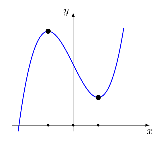
Figure 4: Critical points of $x^{3}-2x+2$ are $\pm\sqrt{2/3}$. There is no direction of descent for $|p(x)|$ at $\sqrt{2/3}$ on the real line.

Figure 5: Polynomiograph of RNM for $z^{3}-1$ (left) and $z^{3}-2z+2$.

Remark 3.

According to RNM polynomiographs of Figure 5 the basins of attraction of the critical points, in the worst-case, appear to be limited to boundaries of the basins of attraction of the roots. Thus even if $z$ is very close to a critical point $c$ and $|p(z)|>|p(c)|$, $|p(\widehat{N}_{p}(z))|$ could drop below $|p(c)|$ so that after one iteration of RNM the new iterates bypass $c$.

4 Proof of Modulus Reduction Theorem

We first to prove two auxiliary lemmas.

Lemma 1.

(Auxiliary Lemma for Selection of Descent Direction) Let $u\in\mathbb{C}$ be nonzero, and $k$ a natural number. Define

$$G_{k}(z)=\overline{u}z^{k}+u{\overline{z}}^{k}.$$ (20)

Treating $u$ as $u_{k}$ in (8), define $\gamma,\delta$ and let $c=c_{k}=\max\{|\gamma|,|\delta|\}$. Next define $\theta$ as in (9). We have

$$G_{k}(\alpha ue^{i\theta})=-c|u|^{2}\alpha^{k}<0,\quad\forall\alpha>0.$$ (21)

Proof.

Since $\gamma=u^{k-1}+\overline{u}^{k-1}$, $\delta=i(u^{k-1}-\overline{u}^{k-1})$, from conjugation, exponentiation and Euler’s formula $e^{i\theta}=\cos\theta+i\sin\theta$, we have

$$G_{k}(\alpha ue^{i\theta})=\alpha^{k}|u|^{2}(\gamma\cos k\theta+\delta\sin k\theta).$$ (22)

Since $\gamma$ and $\delta$ are real and $u\not=0$, $c>0$. Substituting for $\theta$ in (22) proves (21). ∎

Lemma 2.

(Auxiliary Lemma for Step-Size and Estimate of Modulus Reduction) Given $C\in(0,\frac{1}{3}]$ and natural number $k$, define

$$H_{C}(x)=-Cx^{k}+\frac{x^{k+1}}{(1-x)}.$$ (23)

$H_{C}(x)$ is negative and monotonically decreasing on $[0,\frac{1}{3}C]$. Moreover,

$$H_{C}\left(\frac{C}{3}\right)\leq-\frac{3}{2}\bigg{(}\frac{C}{3}\bigg{)}^{k+1}.$$ (24)

Proof.

Differentiating $H_{C}(x)$ we get

$$H_{C}^{\prime}(x)=x^{k-1}\bigg{(}-Ck+\frac{(k+1)x-kx^{2}}{(1-x)^{2}}\bigg{)}.$$ (25)

From (25) it follows that when $x$ is a small positive number, $H_{C}^{\prime}(x)$ is negative so that $H_{C}(x)$ is decreasing at the origin. Since $H_{C}(0)=0$ and $H_{C}(C)>0$, the minimum of $H_{C}(x)$ over $[0,C]$ is attained. Solving $H^{\prime}_{C}(x)=0$, from (25) it follows that the minimizer, $x_{*}$, of $H_{C}(x)$ is the smaller solution of the quadratic equation $a_{2}x^{2}+a_{1}x+a_{0}=0$, where

$$a_{2}=(Ck+k),\quad a_{1}=-(2Ck+(k+1)),\quad a_{0}=Ck.$$ (26)

The roots are

$$\frac{-a_{1}\pm\sqrt{a_{1}^{2}-4a_{0}a_{2}}}{2a_{2}}=\frac{2a_{0}}{-a_{1}\mp\sqrt{a_{1}^{2}-4a_{0}a_{2}}}.$$ (27)

Since $a_{2}a_{0}>0$ the smaller root, say $x_{*}$, is $2a_{0}/(-a_{1}+\sqrt{a_{1}^{2}-4a_{2}a_{0}})\geq-2a_{0}/2a_{1}=-a_{0}/a_{1}$. Substituting for $a_{0}$ and $a_{1}$ and the fact that $C\in(0,\frac{1}{3}]$ we obtain

$$x_{*}\geq\frac{Ck}{2Ck+(k+1)}\geq\frac{Ck}{2k+1}\geq\frac{C}{3}.$$ (28)

Substituting $x=C/3$ into $H_{C}(x)$, using that $H_{C}(x)$ is monotonically decreasing and negative in $[\frac{1}{3}C,x_{*}]$, that $1/(1-C/3)\leq 3/2$, we get

$$H_{C}\left(\frac{C}{3}\right)\leq-3\left(\frac{C}{3}\right)^{k+1}+\frac{3}{2}\left(\frac{C}{3}\right)^{k+1}=-\frac{3}{2}\left(\frac{C}{3}\right)^{k+1}.$$ (29)

Hence the proof. ∎

4.1 Proof of Theorem 1

With $z=z_{0}$, let the parameters $k$, $A=A(z_{0})$, $u_{k}$, $c_{k}$, and $\theta$ be defined according to (7) - (9). Also, let RNM iterate $z_{1}$ and $C_{k}$ be defined as in (10). Set

$$\alpha=\frac{C_{k}}{3|u_{k}|},\quad x=\alpha|u_{k}|=\frac{C_{k}}{3}.$$ (30)

From Definition 1 the RNM iterate is $z_{1}=z_{0}+\alpha u_{k}e^{i\theta}$. We claim $C_{k}\leq 1/3$ and

$$F(z_{1})-F(z_{0})\leq 6A^{2}H_{C_{k}}(x),$$ (31)

where $H_{C}(x)$ is the function defined in Lemma 2. Assuming the validity of the claim, then using the bound (24) in Lemma 2, proof of (13) is immediate. To prove $C_{k}\leq 1/3$, from the definition of $c_{k}$,

$$c_{k}\leq|u_{k}|^{k-1}+|\overline{u}_{k}|^{k-1}=2|u_{k}|^{k-1}.$$ (32)

Also, from the definition of $A=A(z_{0})$, $|u_{k}|\leq A^{2}$. Thus

$$C_{k}=\frac{c_{k}|u_{k}|^{2-k}}{6A^{2}}\leq\frac{2|u_{k}|}{6A^{2}}\leq\frac{1}{3}.$$ (33)

Next we prove (31). With $a_{j}=p^{(j)}(z_{0})/j!$, $j=0,\dots,n$, from Taylor’s theorem we have

$$p(z_{1})=a_{0}+\sum_{j=k}^{n}a_{j}(z_{1}-z_{0})^{j}=a_{0}+\sum_{j=k}^{n}a_{j}(\alpha u_{k}e^{i\theta})^{j}.$$ (34)

We rewrite $p(z_{1})$ as

$$p(z_{1})=a_{0}+a_{k}w^{k}+W,\quad w=\alpha u_{k}e^{i\theta},\quad W=\sum_{j=k+1}^{n}a_{j}w^{j}.$$ (35)

Since $F(z_{1})=p(z_{1})\overline{p(z_{1})}$, from (35) it may be written as the following sum of six terms

$$F(z_{1})=a_{0}\overline{a}_{0}+(a_{0}\overline{a}_{k}\overline{w}^{k}+\overline{a}_{0}a_{k}w^{k})+(a_{0}\overline{W}+\overline{a}_{0}W)+(a_{k}w^{k}\overline{a}_{k}\overline{w}^{k})+(a_{k}w^{k}\overline{W}+\overline{a}_{k}\overline{w}^{k}W)+W\overline{W}.$$ (36)

The first term in (36) is $F(z_{0})$. Using Lemma 1, and since $|w|=x$ and $u_{k}=a_{0}\overline{a_{k}}$, we compute the next term in (36):

$$(a_{0}\overline{a}_{k}\overline{w}^{k}+\overline{a}_{0}a_{k}w^{k})=\alpha^{k}(\overline{u}_{k}u^{k}e^{ik\theta}+u_{k}\overline{u_{k}}^{k}e^{-ik\theta})=G_{k}(\alpha u_{k}e^{i\theta})=-c_{k}\alpha^{k}|u_{k}|^{2}=-c_{k}|u_{k}|^{2-k}x^{k}.$$ (37)

From (36), (37) and the triangle inequality we have

$$F(z_{1})-F(z_{0})\leq-c_{k}|u_{k}|^{2-k}x^{k}+2|\overline{a}_{0}W|+|a_{k}w^{k}|^{2}+2|\overline{a}_{k}\overline{w}^{k}W|+|W|^{2}.$$ (38)

We bound the last four terms in (38). Since $0\leq x<1$ we have

$$\sum_{j=k+1}^{n}x^{j}\leq x^{k+1}\sum_{j=0}^{\infty}x^{j}=\frac{x^{k+1}}{(1-x)}.$$ (39)

From this and definition of $w$, $W$, $a_{j}$ and $A$ we have

$$|\overline{a}_{0}W|\leq A^{2}\frac{x^{k+1}}{(1-x)},\quad|a_{k}w^{k}|^{2}\leq A^{2}x^{2k},\quad|\overline{a}_{k}\overline{w}^{k}W|\leq A^{2}\frac{x^{2k+1}}{(1-x)},\quad|W|^{2}\leq A^{2}\frac{x^{2k+2}}{(1-x)^{2}}.$$ (40)

The first two of the following three inequalities are clear and the third follows since $x=C_{k}/3\leq 1/9$ implies $x^{k+1}\leq(1-x)$.

$$A^{2}x^{2k}\leq A^{2}\frac{x^{k+1}}{(1-x)},\quad A^{2}\frac{x^{2k+1}}{(1-x)}\leq A^{2}\frac{x^{k+1}}{(1-x)},\quad A^{2}\frac{x^{2k+2}}{(1-x)^{2}}\leq A^{2}\frac{x^{k+1}}{(1-x)}.$$ (41)

Using (41) in (40) and subsequently in (38) we obtain the following bound on the decrement in terms of $H_{C_{k}}(x)$:

$$F(z_{1})-F(z_{0})\leq-c_{k}|u_{k}|^{2-k}x^{k}+6A^{2}\frac{x^{k+1}}{(1-x)}=6A^{2}H_{C_{k}}(x).$$ (42)

Then using Lemma 2 in (31) we have the proof of the first inequality in (13) of Theorem 1. Next we prove the second inequality in (13). From the definition of $c_{k}$ in (8) we have

$$c_{k}\geq|u_{k}|^{k-1}.$$ (43)

From (43) and the definition of $C_{k}$ we get

$$C_{k}\geq\frac{|u_{k}|^{k-1}|u_{k}|^{2-k}}{6A^{2}}=\frac{|u_{k}|}{6A^{2}}.$$ (44)

Finally, (44) implies the second inequality in (13). The case of $k=1$, see (14) is straightforward from definitions and the first inequality in (13). The proof of Theorem 1 is now complete.

5 Proof of Global Convergence Theorems

Here we prove theorems 2 and 3.

5.1 Proof of Theorem 2

We prove (i)-(v) in Theorem 2.

(i): It is easy to see $S_{0}$ is a bounded set. In fact an explicit bound on the modulus of its points can be computed. By Theorem 1 for any $z$ in $S_{0}$ the corresponding orbit under RNM remains in $S_{0}$ because the modulus of $p(z)$ decreases from one iteration to the next.

(ii): For any iterate $r<t$, $|p(z_{r})p^{\prime}(z_{r})|\geq\varepsilon$. Then by Theorem 1, $F(z_{r+1})-F(z_{r})\leq\Delta_{\varepsilon}$. The upper bound on $t$ now follows from the inequality $|p(z_{0})|^{2}-t\Delta_{\varepsilon}\leq 0$.

(iii): From Theorem 1 it follows that for any seed $z_{0}$ with $|p(z_{0})|\leq M$ the sequence of $\Delta_{1}(z_{t})$ must converge to zero. But this happens if and only if $p(z_{t})p^{\prime}(z_{t})$ converges to zero. This implies $z_{t}$ converges to a root of $p(z)$.

(iv): Let $\theta$ be a root of $p(z)$. From (iii) it follows that there exists $\rho>0$ such that for any $z_{0}$ in the disc $D_{\rho}(\theta)=\{z:|z-\theta|<\rho\}$, $\widehat{O}^{+}(z)$ converges to some root of $p(z)$. We claim there exists an $\rho$ such that all such orbits converge to $\theta$ itself. Otherwise, there exists a sequence $\{w_{t}:t=1,2,\dots\}$ convergent to $\theta$ such that the corresponding sequence $\{N_{p}(w_{t}):t=1,2,\dots\}$ converges to a root $\theta^{\prime}\not=\theta$. But this cannot happen because $N_{p}(w_{t})=w_{t}-p(w_{t})\overline{p^{\prime}(w_{t})}/9A^{2}(w_{t})$ converges to $\theta$.

(v) The proof of this is the direct consequence of GMP and monotonicity property of RNM.

Remark 4.

Consider the computational complexity of each iteration. If we estimate $A_{0}$, see (ii) in Theorem 2, ignoring this preprocessing, the complexity of each iteration is essentially that of computing $p(z)$ and $p^{\prime}(z)$ in $O(n)$ operations (e.g. by Horner’s method). Computing the normalized derivatives $|p^{(j)}(z)|/j!$, hence $A(z)$, in each iteration via straightforward algorithm takes $O(n^{2})$ operations. However, these can be computed efficiently in $O(n\log n)$ operations, see Pan [16]. A practical strategy is to evaluate the normalized derivatives in every so many iterations, using an estimate for the maximum of their modulus in computing $\widehat{N}_{p}(z)$.

5.2 Proof of Theorem 3

If the sequence $z_{t}$ of modified RNM iterates (Algorithm 2) approaches a critical point, say $c$, then it must be the case that when $t$ is large enough the sequence of indices $\overline{k}$ corresponding to $\overline{z}_{t+1}=\overline{N}_{p}(z_{t})$ will coincide with the index $k$ at $c$. While the corresponding angles $\theta$ defined in (9) may be different from the angle corresponding to $c$, by continuity $F(\overline{z}_{t+1})-F(z_{t})$ must closely approximate $F(\overline{z}_{t+1})-F(c)$ and hence will approximate the decrement corresponding to $c$, namely $\Delta_{k}(c)$ assured by Theorem 1. This implies for some $t$ the inequality $F(\overline{z}_{t+1})-F(z_{t})\leq 0.5\Delta_{\overline{k}}(z_{t})$ will be satisfied. Moreover, as $z_{t}$ gets closer ro $c$, $F(\overline{z}_{t+1})<F(c)$. In summary, after a finite number of iterations of the modified RNM, we must have $|p(z_{t})|<|p(c)|$ so that RNM iterates will bypass $c$. As there are at most $n-1$ critical points, the orbit of modified RNM will bypass all critical points and converge to a root of $p(z)$. This completes the proof of Theorem 3.

6 Further Algorithmic Considerations

In this section we remark on some improvements and applications of the RMN.

6.1 Improving Iteration Complexity

From Theorem 2 in $O(1/\varepsilon^{2})$ iterations of RNM we have an iterate $z_{t}$ such that either $|p(z_{t})|\leq\varepsilon$ or $|p(z_{t})p^{\prime}(z_{t})\leq\varepsilon$. When $z_{t}$ satisfies the first condition we would expect the number of iterations to be better than $O(1/\varepsilon^{2})$. This is because locally Newton’s method converges quadratically and reduces the polynomial modulus as well. Thus once an iterates enter such a region very few subsequent iterations are needed. On the one hand, at the cost of one additional function evaluation we can compare the RNM iterate and Newton iterate and choose the iterate with smaller $|p(z)|$ value. On the other hand, we can check Smale’s approximate zero theory explained next. The only time the number of iterations may be large is when the iterates converge to a critical point. However, even in this case the modified RNM checks if $|p^{\prime}(z_{t})|$ is small and if so by treating $z_{t}$ as a near-critical point it bypassed the critical point to which the RNM iterates may be converging to and in doing so the orbit avoids the critical point for good.

6.2 Combining RNM and Smale’s Approximate Zero Theory

It is well-known that Newton’s method has locally quadratic rate of convergence to a simple root. Smale’s approximate zero theory [19] gives a sufficient condition for membership of a point in the quadratic region of convergence. Specifically, the orbit of $z_{0}$ satisfies $|z_{j}-\theta|\leq.5^{2^{j}}|z_{0}-\theta|$ for some root $\theta$ of $p(z)$, provided the following condition holds at $z_{0}$

$$\alpha(z_{0})\equiv\beta(z_{0})\gamma(z_{0})\leq\alpha_{0}=\frac{1}{4}({13-3\sqrt{7}})\approx 0.157,$$ (45)

where

$$\beta(z_{0})\equiv\left|\frac{p(z_{0})}{p^{\prime}(z_{0})}\right|,\quad\gamma(z_{0})\equiv\max\left\{\left|\frac{p^{(j)}(z_{0})}{j!p^{\prime}(z_{0})}\right|^{1/(j-1)}:j=2,\dots,n\right\}.$$ (46)

We can thus check (45) in every iteration of RNM or modified RNM. Observe that since $z_{0}$ must be a noncritical point, Smale’s condition can alternatively be written as

$$|p(z_{0})\overline{p^{\prime}(z_{0})}|\leq\rho(z_{0})\equiv\frac{\alpha_{0}|p^{\prime}(z_{0})|^{2}}{\gamma(z_{0})}.$$ (47)

Note that from (8) $u_{1}(z_{0})=p(z_{0})\overline{p^{\prime}(z_{0})}$, the quantity that determines the decrement in RNM (Theorem 1). Thus at an iterate $z_{0}$, when $|p(z_{0})\overline{p^{\prime}(z_{0})}|$ is large enough Theorem 1 implies there is a sufficient reduction in the modulus of the next iterate of RNM. And when $|p(z_{0})\overline{p^{\prime}(z_{0})}|$ is small enough, $z_{0}$ lies in the quadratic region of convergence of some root of $p(z)$. We can also write (47) as

$$|p(z_{0})|\leq\sigma(z_{0})\equiv\frac{\alpha_{0}|p^{\prime}(z_{0})|}{\gamma(z_{0})}.$$ (48)

While we cannot estimate the number of iterations to enter the region of convergence of a root, when $|p^{\prime}(z_{0})|$ is below the threshold, $\sigma(z_{0})$ is bounded away from zero, independent of $\varepsilon$. Once an iterate is sufficiently away from a critical point and its polynomial modulus satisfies (48), by Smale’s theory in only a few more iterations of Newton’s method, namely $O(\log\log(1/\varepsilon))$ iterations, we would get an Newton’s iterate to within $\varepsilon$ distance of a root of $p(z)$. In summary, RNM and its modified version complement Smale’s one-point theory, resulting in a globally convergent method that enjoys quadratic rate of convergence.

6.3 Computing All Roots

Computing all roots of a complex polynomial is a significant problem both in theory and practice. One of the classical algorithms for the problem is Weyl’s algorithm, a two-dimensional version of the bisection algorithm (see [16]) that begins with an initial suspect square containing all the roots. The square is subsequently partitioned into four congruent subsquares and via a proximity test some squares are discarded and the remaining squares are recursively partitioned into four congruent subsquares and the process is repeated. Once close enough to a root, Newton’s method will be used to compute accurate approximations efficiently. For detail on theoretical and some practical algorithms, see in Pan [16] and Bini and Robol [2]. Hubbard et al. [6] show all roots of a polynomial can be computed solely via Newton’s method. Specifically, it is shown that for polynomials of degree $n$, normalized so that all roots lie in the complex unit disc, there is an explicit set of $1.1n(\log n)^{2}$ seeds whose orbits are guaranteed to find all roots of such polynomials via Newton’s method. Schleicher and Stoll [18] show further results and computational experiments with large degree polynomials.

While we do not offer computational results for computing all roots via RNM or modified RNM, here we describe how it may be combined with deflation in order to compute all roots of a polynomial $p(z)$. Suppose we have computed an approximation $\widehat{\theta}$ to a root $\theta$ of $p(z)$. As is done in ordinary deflation, dividing $p(z)$ by $(z-\widehat{\theta})$ we get $p(z)=(z-\widehat{\theta})q(z)+r(z)$. By continuity, the roots of $q(z)$ approximate the remaining roots of $p(z)$. If we now apply the RNM to $q(z)$, starting at $\widehat{\theta}$, the iterates will approximate a root of $q(z)$. Once sufficiently iterated, we should witness the iterates getting father away from $\widehat{\theta}$. Then we begin iterating $p(z)$ itself and this, by virtue of modulus reduction property of RNM, will in turn approximate a root of $p(z)$, different from the one approximated by $\widehat{\theta}$. More generally, assuming we have obtained approximation $\widehat{\theta}_{1},\dots,\widehat{\theta}_{m}$ to $m$ roots of $p(z)$, we divide $p(z)$ by $w(z)=(z-\widehat{\theta}_{1})\times\cdots\times(z-\widehat{\theta}_{m})$ and apply the procedure to the new quotient polynomial. In order to make the algorithm more effective one may first compute tight bounds on the roots, see [9] and [8]. This simple scheme combined with RNM could enhance standard deflation with standard Newton’s method. Future experimentation with such approach could determine the effectiveness of the method.

Concluding Remarks and Links to Experimental Codes

In this article we have considered minimization of the modulus of a real or complex polynomial as a basis for computing its roots. Using this objective, together with utilization of the Geometric Modulus Principle, we developed a stronger version of the classical Newton’s method, called the Robust Newton Method (RNM), where the orbit of an arbitrary seed converges, either to a root or critical point of the underlying polynomial. Each iteration monotonically reduces the polynomial modulus with an a priori estimate. We also described a modified RNM that avoids critical points, converging only to roots. The results are self-contained, accessible to educators and students, also useful for researchers. Pedagogically, the article introduces novel results regarding Newton’s method, including a simple proof of the FTA, and a convergent iterative algorithm for solving a cubic equation. In fact in a graduate numerical analysis class the author proposed research projects based on the implementation of RNM and the polynomiographs based on RNM presented here are based on one such project. In another project, to be released later, students produced an online website that computes all roots of a polynomial for small size polynomials. Theoretically, based on estimate of modulus reduction, we have justified that the iteration complexity to compute an approximate zero is independent of the degree of the polynomial, dependent only on the desired tolerance, $\varepsilon$. At the same time RNM is complementary to Smale’s theory of approximate zeros, resulting in an algorithm that is globally convergent while locally it enjoying quadratic rate of convergence at simple roots. RNM and modified RNM can be used to compute all roots of a polynomial by themselves or in combination with other algorithms, such as [16], [6] and [18]. These suggest several areas of research and experimentation, including development of new algorithms for computing all roots, extending RNM to more general iterative methods. Finally, visualization of RNM, as demonstrated in a few example here, result in images distinct from the existing fractal and non-fractal polynomiographs such as those in [10]. In particular, RNM smooths out the fractal boundaries of basins of attraction. In conclusion we give two links to experimental codes carried out by students, one for generating polynomiographs of RNM and another for computing all roots of small degree polynomials. These are available at https://github.com/baichuan55555/CS510-Project-1 and https://github.com/fightinglinc/Robust-Newton-Method, respectively. However, we believe RNM and its modifications would invite the readers to carry out their own experimentation and further investigations.

Acknowledgements

I would like to thank some of my students, Matthew Hohertz for carefully reading an earlier version and making useful comments. Also two groups of students in my graduate numerical analysis course, Baichuan Huang, Jiawei Wu, and Zelong Li for generating the relevant polynomiographs in the article, also Linchen Xie and Shanao Yan for producing an applet to compute all roots of small degree polynomial. The github links are given above.

References

- [1] Beardon, A. F. (1991). Iteration of Rational functions: Complex Analytic Dynamical Systems. New York: Springer-Verlag.
- [2] D. A. Bini and L. Robol, Solving secular and polynomial equations: a multiprecision algorithm . Journal of Computational and Applied Mathematics 272 (2014), 276-292.
- [3] Blum, L., Cucker, F., Shub, M. and Smale, S. (1998). Complexity and Real Computation. Springer-Verlag, New York.
- [4] Cayley, A. (1879). The Fourier imaginary problem. American Journal of Mathematics. 2: 97.
- [5] Fine, B. and Rosenberger, G. (1997). The Fundamental Theorem of Algebra. New York: Springer-Verlag.
- [6] Hubbard, J., Schleicher, D. Sutherland, S. (2001). How to find all roots of complex polynomials by Newton’s method. Inventiones Mathematicae. (146): 1 - 33.
- [7] Irving, R. (2013). Beyond the Quadratic Formula. The Mathematical Association of America.
- [8] Jin, Yi. (2006). On efficient computation and asymptotic sharpness of Kalantari’s bounds for zeros of polynomials, Mathematics of Computation (75): 1905 - 1912.
- [9] Kalantari, B. (2005). An infinite family of bounds on zeros of analytic functions and relationship to Smale’s bound. Mathematics of Computation. 74: 841 - 852.
- [10] Kalantari, B. (2008). Polynomial Root-Finding and Polynomiography. Hackensack, NJ: World Scientific.
- [11] Kalantari, B. (2011). A geometric modulus principle for polynomials. Amer. Math. Monthly. 118: 931 - 935.
- [12] Kalantari, B. (2014). A One-line proof of the Fundamental Theorem of Algebra with Newton’s Method as a consequence. http://arxiv.org/abs/1409.2056,.
- [13] Körner, T. W. (2006). On the fundamental theorem of algebra. Amer. Math. Monthly. 113: 347 - 348.
- [14] Littlewood, J. E. (1941). Mathematical notes (14): Every polynomial has a root. J. London Math. Soc. 16: 95 - 98.
- [15] Oliveira, O. R. B. (2011). The fundamental theorem of algebra: an elementary and direct proof. Math. Intelligencer. (33)2: 1 - 2.
- [16] Pan, V. Y. (1997). Solving a polynomial equation: some history and recent progress, SIAM Review. 39: 187 - 220.
- [17] Peitgen, H.-O., Saupe, D. and Haeseler, F. von. (1984). Cayley’s problem and Julia sets. Math. Intelligencer 6(2): 11 - 20.
- [18] D. Schleicher and R, Stoll, Newtons method in practice: finding all roots of polynomials of degree one million efficiently, Journal of Theoretical Computer Science 681 (2017), 146-166.
- [19] Smale. S. (1986). Newton’s method estimates from data at one point. The Merging disciplines: New directions in pure, applied, and computational mathematics, Springer: 185 - 196.