Elmachtoub, Liang, McNellis

Decision Trees for Decision-Making under the Predict-then-Optimize Framework

Decision Trees for Decision-Making under the Predict-then-Optimize Framework

Adam N. Elmachtoub Department of Industrial Engineering and Operations Research and Data Science Institute, Columbia University, NY, USA adam@ieor.columbia.edu Jason Cheuk Nam Liang Operations Research Center, Massachusetts Institute of Technology, MA, USA
jcnliang@mit.edu Ryan McNellis Department of Industrial Engineering and Operations Research and Data Science Institute, Columbia University, NY, USA
Amazon, NY, USA
rtm2130@columbia.edu, rmcnell@amazon.com

We consider the use of decision trees for decision-making problems under the predict-then-optimize framework. That is, we would like to first use a decision tree to predict unknown input parameters of an optimization problem, and then make decisions by solving the optimization problem using the predicted parameters. A natural loss function in this framework is to measure the suboptimality of the decisions induced by the predicted input parameters, as opposed to measuring loss using input parameter prediction error. This natural loss function is known in the literature as the Smart Predict-then-Optimize (SPO) loss, and we propose a tractable methodology called SPO Trees (SPOTs) for training decision trees under this loss. SPOTs benefit from the interpretability of decision trees, providing an interpretable segmentation of contextual features into groups with distinct optimal solutions to the optimization problem of interest. We conduct several numerical experiments on synthetic and real data including the prediction of travel times for shortest path problems and predicting click probabilities for news article recommendation. We demonstrate on these datasets that SPOTs simultaneously provide higher quality decisions and significantly lower model complexity than other machine learning approaches (e.g., CART) trained to minimize prediction error.

prescriptive analytics; data-driven optimization; machine learning; decision trees

1 Introduction

Many decision-making problems of interest to practitioners can be framed as optimization problems containing uncertain input parameters to be estimated from data. For example, personalized advertising requires estimation of click/conversion probabilities as a function of user features, portfolio optimization problems necessitate accurate predictions of asset returns, and delivery routing problems require forecasts of travel times. A convenient and widely-utilized framework for addressing these problems is the predict-then-optimize framework. Predict-then-optimize is a two step approach which (i) first predicts any uncertain input parameters using a machine learning (ML) model trained on historical data, and (ii) then generates decisions by solving the corresponding optimization problem using the predicted parameters. Typically, the ML models in this framework are trained using loss functions measuring prediction error (e.g., mean squared error) without considering the impact of the predictions on the downstream optimization problem. However, for many practitioners, the primary interest is in obtaining near-optimal decisions from the input parameter estimates rather than minimizing prediction error. In this work, we provide a methodology for training decision trees, under the predict-then-optimize framework, to minimize decision error rather than prediction error.

A natural idea is to integrate the prediction task with the optimization task, training the ML models using a loss function which directly measures the suboptimality of the decisions induced by the predicted input parameters. elmachtoub2017smart propose such a loss function for a broad class of decision-making problems, which they refer to as the Smart Predict-then-Optimize loss (SPO loss). However, the authors note that training ML models using SPO loss is likely infeasible due to the SPO loss function being nonconvex and discontinuous (and therefore not differentiable). The authors therefore propose a convex surrogate loss function they refer to as SPO+ loss, which they show is Fisher consistent with respect to SPO loss under some assumptions. wilder2019melding also note the nondifferentiability of SPO loss and modify the objective function of the nominal optimization problem to derive a differentiable, surrogate loss function. Both works demonstrate empirically that training ML models using the surrogate loss functions yields better decisions than models trained to minimize prediction error. However, the surrogate loss functions are not guaranteed to recover optimal decisions with respect to SPO loss and merely serve as approximations for computational feasibility. A practical and general methodology for training ML models using SPO loss directly has not yet been proposed.

In this work, we present algorithms for training decision trees to minimize SPO loss, which we call SPO Trees (SPOTs). Despite the nonconvexity and discontunity of the SPO loss function, we show that the optimization problem for training decision tree models with respect to SPO loss can be greatly simplified through exploiting certain structural properties of decision trees. Therefore, to the best of our knowledge, we provide the first tractable methodology for training an ML model using SPO loss for a general class of decision-making problems. Decision trees are typically trained using “greedy” recursive partitioning approaches to minimize prediction error such as the popular CART algorithm (breiman1984classification); several recent works have also proposed integer programming strategies for training decision trees to optimality (bertsimas2017optimal, gunluk2018optimal, verwer2019learning, hu2019optimal, aghaei2020learning). We propose tractable extensions of the greedy and integer programming methodologies from the literature to train decision trees using SPO loss. We also provide methodology for training an ensemble of SPO Trees to boost decision performance, which we refer to as SPO Forests. We conduct several numerical experiments on synthetic and real data demonstrating that SPOTs simultaneously find higher quality decisions while exhibiting significantly lower model complexity (i.e., depth) than other tree-building approaches trained to only minimize prediction error (e.g., CART). Implementations of our algorithms and experiments may be found at https://github.com/rtm2130/SPOTree.

We remark that the use of decision trees for decision-making problems has seen increased attention in practice and recent literature due to their interpretability (kallus2017recursive, elmachtoub2017practical, ciocan2018interpretable, bertsimas2019optimal, aghaei2019learning, aouad2019market). Decision trees for decision-making are seen as interpretable since their splits which map features to decisions are easily visualized. One of our key findings is that SPOTs end up being even more interpretable than trees trained to minimize prediction error as they require significantly less leaves to yield high-quality decisions. Finally, we note that decision trees exhibit several desirable properties as estimators. Namely, they are nonparametric, allowing them to capture nonlinear relationships and interaction terms which would have to be manually specified in other models such as linear regression.

1.1 Literature Review

There have been several approaches proposed in the recent literature for training decision tree models for optimal decision-making. bertsimas2019predictive show how to properly leverage ML algorithms, including decision trees, in order to yield asymptotically optimal decisions to a class of stochastic optimization problems. However, their decision trees are trained in the same procedure as CART (but applied differently) and thus do not take into consideration the structure of the underlying decision-making problem. There has also been several recent works on training decision trees for personalizing treatments among a finite set of possible options. kallus2017recursive uses a loss function for training their trees which maximizes the efficacy of the recommended treatments rather than minimizing prediction error. bertsimas2019optimal consider a similar treatment recommendation problem, but their approach uses an objective function involving a weighted combination of prediction and decision error. Our approach considers a more general class of decision-making problems potentially involving a large number of decisions represented by a general feasible region. aghaei2019learning propose methodology for training decision trees for decision-making problems using a loss function which penalizes predictions that discriminate on sensitive features such as race or gender. However, their loss function does not consider the impact of predictions on downstream decisions, instead seeking to minimize prediction error.

We also summarize a few additional approaches proposed in the literature which successfully apply other types of ML models to decision-making problems. kao2009directed propose a loss function for training linear regression models which minimizes a convex combination between the prediction error and decision error. In addition to not considering decision tree models, their setting considers only quadratic optimization problems with no constraints. donti2017task provide a more general methodology related to this line of work that relies on differentiating the optimization problem. wilder2019end consider the problem of optimizing a function whose input is a graph structure that is unknown but can be estimated through prediction. Their end-to-end learning procedure involves constructing a simpler optimization problem in continuous space as a differentiable proxy for the more complex graph optimization problem. wilder2019melding, mandi2019smart consider training ML models using “decision-focused” loss functions for various combinatorial optimization problems; their methods do not attempt to minimize SPO loss directly but rather employ simpler surrogate loss functions. demirovic2019predict+ propose methodology for training linear regression models to directly minimize SPO loss, but their approach is specialized for ranking optimization problems. By contrast, we propose methodology for training decision trees under SPO loss for a more general class of optimization problems (which subsumes ranking problems as a special case).

2 The Predict-then-Optimize Framework

In this section, we summarize the predict-then-optimize framework and the SPO loss proposed in elmachtoub2017smart. We focus on a general class of decision-making problems which can be described by an optimization problem with known constraints and an unknown linear objective function (at the time of solving) which can be predicted from feature data. Many relevant problems of interest fall under this general structure, include predicting travel times for shortest path problems, predicting demand for inventory management problems, and predicting returns for portfolio optimization.

We let $S\subseteq\mathbb{R}^{d}$ denote the feasible region for the decisions, where $d$ is the dimension of the decision space. The decision-making problem can then defined mathematically as $z^{*}(c)=\min_{w\in S}c^{T}w$, where $c\in\mathbb{R}^{d}$ is a cost vector of the optimization problem and $w\in\mathbb{R}^{d}$ is the vector of decision variables. Let $W^{*}(c)=\argmin_{w\in S}\{c^{T}w\}$ denote the set of optimal decisions corresponding to $z^{*}(c)$, and let $w^{*}(c)$ denote an arbitrary individual member of the set $W^{*}(c)$. It is assumed that $S$ is specified in such a way that the computation of $w^{*}(c)$ and $z^{*}(c)$ are tractable for any cost vector $c$; for example, commercial optimization solvers are known to capably solve optimization problems with linear, conic, and/or integer constraints.

In the predict-then-optimize framework, the true cost vector is not known at the time of solving $w^{*}(\cdot)$ for an optimal decision, and thus a predicted cost vector $\hat{c}$ is used instead. Our predictions will rely on training a ML model from a given dataset $\{(x_{1},c_{1}),(x_{2},c_{2}),...,(x_{n},c_{n})\}$, where $x\in\mathbb{R}^{p}$ denote a vector of $p$ features available for predicting $c$. The $n$ feature-cost samples in the dataset are assumed to be independently and identically distributed according to an unknown joint distribution on $x$ and $c$. Let $\mathcal{H}$ denote a hypothesis class of candidate ML models $f:\mathbb{R}^{p}\rightarrow\mathbb{R}^{d}$ for predicting cost vectors from feature vectors, where $\hat{c}=f(x)$ is interpreted as the predicted cost vector associated with feature vector $x$ for model $f$. Finally, let $\ell(\cdot,\cdot):\mathbb{R}^{d}\times\mathbb{R}^{d}\rightarrow\mathbb{R}_{+}$ denote the loss function used to train the ML models, where $\ell(\hat{c},c)$ scores the loss incurred by a prediction of $\hat{c}$ when the true cost vector is $c$. Given a specified hypothesis class $\mathcal{H}$ and loss function $\ell(\cdot,\cdot)$, the ML models are trained through solving the following empirical risk minimization problem:

$$f^{*}=\argmin_{f\in\mathcal{H}}\quad\frac{1}{n}\sum_{i=1}^{n}\ell(f(x_{i}),c_{i})$$ (1)

In words, the trained ML model $f^{*}$ is the model in the hypothesis class $\mathcal{H}$ which achieves the smallest average loss on the training data with respect to the given loss function $\ell(\cdot,\cdot)$. When presented with a new feature vector $x$, the model $f^{*}$ can be applied in predicting a cost vector $\hat{c}=f^{*}(x)$, and an optimal decision $w^{*}(\hat{c})$ is then proposed using the prediction $\hat{c}$.

One common loss function is mean squared error (MSE) loss, defined as $\ell_{MSE}(\hat{c},c):=||\hat{c}-c||_{2}^{2}$. By comparison, SPO loss scores predicted costs not by their prediction error but rather by the quality of the decisions that they induce. Mathematically, SPO loss measures the excess cost $c^{T}w^{*}(\hat{c})-z^{*}(c)$ incurred from making the (potentially) sub-optimal decision $w^{*}(\hat{c})$ implied by prediction $\hat{c}$ when the true cost is $c$. Note that $W^{*}(\hat{c})$ may contain more than one optimal solution associated with $\hat{c}$. Therefore, elmachtoub2017smart define SPO loss with respect to the worst-case decision from a predicted cost vector $\hat{c}$, defined mathematically below:

$$\ell_{SPO}(\hat{c},c):=\max_{w\in W^{*}(\hat{c})}\{c^{T}w\}-z^{*}(c)\,.$$ (2)

The authors note that training ML models under SPO loss directly is likely infeasible, as SPO loss is nonconvex and discontinuous (and thus not differentiable) with respect to a given prediction $\hat{c}$. Therefore, the authors instead provide an algorithm for training linear models using a convex surrogate loss function called SPO+ loss. wilder2019melding also note the nondifferentiability of SPO loss and modify the objective function of the nominal optimization problem to derive a differentiable, surrogate loss function. In contrast to prior work, we provide multiple strategies for training decision trees using the SPO loss function directly. Our methodology is presented in Section 4.

3 Decision Trees for Decision-Making

In this work, we utilize decision trees under the predict-then-optimize framework. To illustrate this concept, we consider a simple shortest path problem in a graph with two nodes and two candidate roads between them, each with unknown travel times (edge costs) $c_{1}$ and $c_{2}$. We assume that there are $p=3$ features available for predicting edge costs: $x_{1}$ is a binary feature to indicate a weekday, $x_{2}$ is the current hour of the day, and $x_{3}$ is a binary feature to indicate snowfall. The goal is to choose the path with the smallest cost given the observed features. An example of a decision tree applied to this problem is provided in Figure 1, although we note the same logic applies to an arbitrarily sized shortest path graph. Decision trees partition the feature space $\mathbb{R}^{p}$ through successive splits on components of the feature vector $x$. Each split takes the form of a yes-or-no question with respect to a single component. Continuous or ordinal features are split using inequalities, and categorical features are split using equalities. The partitions of $\mathbb{R}^{p}$ resulting from the decision tree splits are referred to as the leaves of the tree. Each leaf assigns a single predicted cost vector $\hat{c}$ and associated decision $w^{*}(\hat{c})$ to all feature vectors which map to that leaf. We define the depth of a leaf as the number of splits taken to reach that leaf. The depth of the tree is defined as the maximum of the depths of its leaves.

Figure 1: Decision tree for a shortest path problem with two edges.

Decision trees are widely regarded as being very interpretable machine learning models, as the mapping from features to costs/decisions may be easily visualized and analyzed for insights. For example, in the decision tree of Figure 1, the second leaf from the left corresponds to the splits $x_{2}<10$, $x_{1}=1$, and $x_{2}\geq 7$, which may be interpreted as the tree determining whether it is currently morning rush hour (i.e., a weekday between 7am and 10am).

3.1 An Illustrative Example

We provide a simple example to illustrate the behavior of decision trees trained using SPO loss versus MSE loss (i.e., SPOTs versus CARTs). We again consider the two edge shortest path problem from before, although we now assume there is only a single continuous feature $x$ available for predicting the travel times of the two edges. We generate a dataset of 10000 feature-cost pairs by (1) sampling 10000 feature values from a Uniform(0,1) distribution, and (2) computing each feature’s associated edge cost by the equations $c_{1}=5x+1.9$ and $c_{2}=(5x+0.4)^{2}$ with no noise for the sake of illustration. We then train a decision tree to minimize SPO loss on this dataset, employing the SPOT training methods detailed in the next section. For sake of comparison, we also train a CART decision tree on the same dataset. CARTs are trained to minimize prediction error, specifically, mean-squared error in our experiments.

(a) SPOT (Depth 1)

(b) CART (Depth 1)

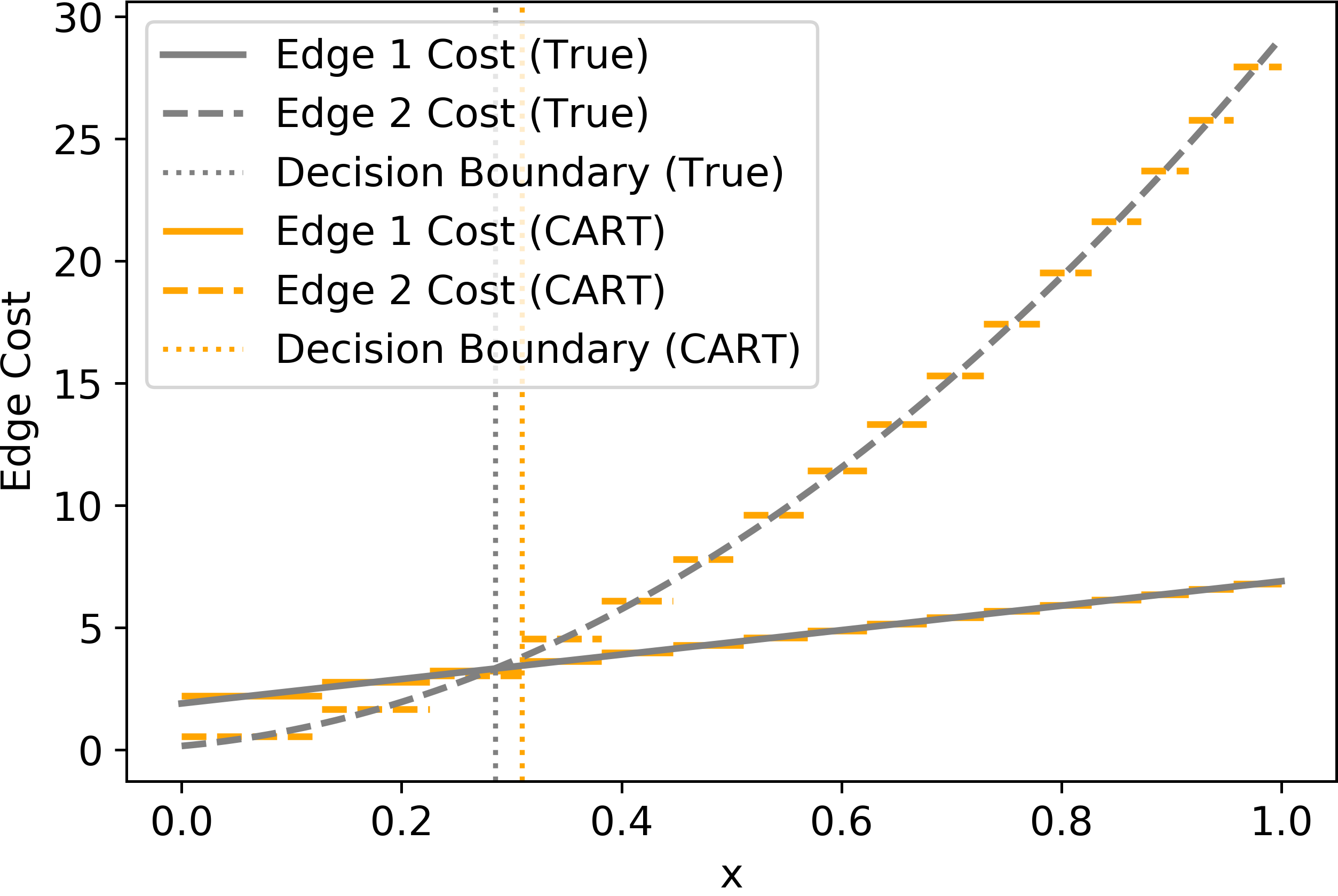
(c) CART (Depth 4)

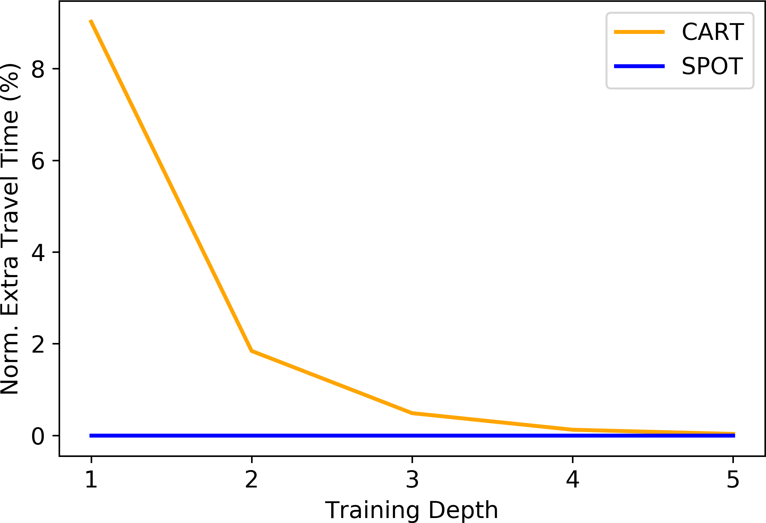
(d) SPOT vs CART Loss

Figure 2: Predictive and decision performance of SPOT and CART decision trees. Figures (a)-(c) visualize the cost predictions of SPOT (blue) and CART (orange) alongside the true cost values (grey). Figure (d) plots the normalized extra travel time of the algorithms as a function of their trained tree depth.

The predictive and decision performance of the SPOT and CART training algorithms are given in Figure 2. Figures 2(a)-2(c) visualize the cost predictions of the SPOT and CART algorithms and compare them against the true unknown edge costs. The two edge costs are equal at $x=0.28$, at which point the optimal decision switches from taking edge 2 to taking edge 1. We therefore refer to the point $x=0.28$ as the optimal or true decision boundary, and is referenced in the figures as a grey vertical line. We also include in the figures the decision boundaries implied by the cost predictions of the SPOT and CART algorithms.

As shown in Figure 2(a), the SPO Tree immediately identifies the correct decision boundary through the split “$x<0.28$”. This behavior is unsurprising, as any other individual split would have resulted in a suboptimal SPO loss incurred on the training set. Each leaf of the SPO tree yields a single predicted cost vector, which is visualized by the flat prediction lines in the regions “$x<0.28$” and “$x\geq 0.28$” of the figure.

Figures 2(b) and 2(c) show the cost vector predictions of the CART algorithm. When trained to a depth of 1 (i.e., a single split), CART results in a severely incorrect decision boundary at $x=0$. This occurs because CART splits at $x<0.62$, and in each of the resulting leaves from this split edge 2 is predicted to have a higher cost than edge 1. Therefore the CART algorithm incorrectly predicts that path 1 is always optimal, resulting in the decision boundary of $x=0$. The CART algorithm does not split on the optimal decision boundary because this is not the split which minimizes cost prediction error on the training set. Consequently, although the cost predictions of CART may be more accurate, the implied shortest path decisions are suboptimal for a significant percentage (28%) of feature values.

As shown in Figure 2(c), when CART is permitted to utilize more splits up to a tree depth of 4, it is able to nearly recover the optimal decision boundary. Even though each individual split taken by CART has less value for decision-making, the splits in combination finely partition the feature space into small enough regions that the predicted cost vectors are highly accurate within each region. Therefore, when trained to a significant depth, CARTs – and more generally, decision trees – potentially have a high enough model complexity to achieve near perfect predictions which translate into near perfect decisions. However, in settings with limited training data, it is no longer possible to train decision trees to a suitably high depth, as a sufficient number of training observations per leaf are required to estimate the leaf cost predictions accurately. Therefore, in these settings, maximizing the contribution of each decision tree split to optimal decision-making becomes a higher priority. Moreover, lower depth decision trees are often preferred for their interpretability and reduced risk of overfitting.

Figure 2(d) assesses the decisions from the SPOT and CART algorithms when trained to different tree depths. The decisions are scored on a held out set of data using the metric of “normalized extra travel time”, defined as the cumulative SPO loss normalized by the cumulative optimal decision costs. $\sum_{i=1}^{n}\ell_{SPO}(\hat{c}_{i},c_{i})/\sum_{i=1}^{n}z^{*}(c_{i})$. Unsurprisingly, the SPO Tree achieves zero decision error at all training depths since it correctly identified the decision boundary at depth 1. By comparison, the CART algorithm exhibits comparatively high decision error at depths 1-3 and only begins to reach a decision error near zero at depth 4. Therefore, the SPO Tree achieves high quality decisions while also being significantly less complex than the CART tree required for comparable decision quality. We show in Section LABEL:sec:Results that this behavior is consistently observed across a range of synthetic and real datasets.

4 Methodology

We now propose several algorithms for training decision trees using the SPO loss function, and we call the resulting models SPO Trees (SPOTs). The objective of any decision tree training algorithm is to partition the training observations into $L$ leaves, $R_{1},...,R_{L}:=R_{1:L}$, whose predictions collectively minimize a given loss function:

$$\min_{R_{1:L}\in\mathcal{T}}\frac{1}{n}\sum_{l=1}^{L}\left(\min_{\hat{c_{l}}}\sum_{i\in R_{l}}\ell(\hat{c_{l}},c_{i})\right)$$ (3)

Above, the constraint $R_{1:L}\in\mathcal{T}$ indicates that the allocation of observations to leaves must follow the structure of a decision tree (i.e., determined through repeated splits on the feature components). The CART algorithm greedily selects tree splits which individually minimize this objective with respect to mean squared error prediction loss (breiman1984classification). More recently, integer programming strategies have been proposed for optimally solving (3) with respect to classification loss (bertsimas2017optimal, gunluk2018optimal, verwer2019learning, hu2019optimal, aghaei2020learning). We next describe tractable extensions of these greedy and integer programming methodologies from the literature to train decision trees using SPO loss, which has been shown to have favorable generalization bounds in several settings (el2019generalization).

elmachtoub2017smart note that training machine learning models under SPO loss is likely infeasible due to the loss function being nonconvex and discontinuous in the predicted cost vectors. However, we show that optimization problem (3) for training decision trees under SPO loss can be greatly simplified through Theorem 4.1, which states that the average of the cost vectors corresponding to a leaf node minimizes the SPO loss in that leaf node.

Theorem 4.1

Let $\bar{c}_{l}:=\frac{1}{|R_{l}|}\sum_{i\in R_{l}}c_{i}$ denote the average cost of all observations within leaf $l$. If $\bar{c}_{l}$ has a unique minimizer in its corresponding decision problem, then $\bar{c}_{l}$ minimizes within-leaf SPO loss. More simply, if $|W^{*}(\bar{c}_{l})|=1$, then $\bar{c}_{l}=\argmin_{\hat{c_{l}}}\sum_{i\in R_{l}}\ell_{SPO}(\hat{c_{l}},c_{i})$.

Proof 4.2

Proof: Let $\bar{c}_{l}$ be defined as stated in the theorem. We will show that the within-leaf SPO loss associated with predicting $\bar{c}_{l}$ lower bounds that of predicting any other feasible cost vector $\hat{c}_{l}\in\mathbb{R}^{d}$. Let $N_{l}=|R_{l}|$ denote the number of observations within leaf $l$. The following holds for any $\hat{c}_{l}\in\mathbb{R}^{d}$:

$$\frac{1}{N_{l}}\sum_{i\in R_{l}}\ell_{SPO}(\bar{c}_{l},c_{i})-\frac{1}{N_{l}}\sum_{i\in R_{l}}\ell_{SPO}(\hat{c}_{l},c_{i})$$

$$~{}=~{} \frac{1}{N_{l}}\sum_{i\in R_{l}}\max_{w\in W^{*}(\bar{c}_{l})}\{c_{i}^{T}w\}-\frac{1}{N_{l}}\sum_{i\in R_{l}}\max_{w\in W^{*}(\hat{c}_{l})}\{c_{i}^{T}w\}$$

$$~{}=~{} \frac{1}{N_{l}}\sum_{i\in R_{l}}c_{i}^{T}w^{*}(\bar{c}_{l})-\frac{1}{N_{l}}\sum_{i\in R_{l}}\max_{w\in W^{*}(\hat{c}_{l})}\{c_{i}^{T}w\}\quad\left(W^{*}(\bar{c}_{l})=\{w^{*}(\bar{c}_{l})\}\text{ is a singleton}\right)$$

$$~{}\leq~{} \frac{1}{N_{l}}\sum_{i\in R_{l}}c_{i}^{T}w^{*}(\bar{c}_{l})-\max_{w\in W^{*}(\hat{c}_{l})}\bigg{\{}\frac{1}{N_{l}}\sum_{i\in R_{l}}c_{i}^{T}w\bigg{\}}$$

$$~{}=~{} \bar{c}_{l}^{T}w^{*}(\bar{c}_{l})-\max_{w\in W^{*}(\hat{c}_{l})}\{\bar{c}_{l}^{T}w\}$$

$$~{}\leq~{} 0\quad\left(\text{by definition of }w^{*}(\bar{c}_{l})\right)$$

We have thus demonstrated that $\bar{c}_{l}$ achieves a within-leaf SPO loss lower or equal to that of any other cost vector $\hat{c}_{l}\in\mathbb{R}^{d}$, thereby proving the theorem.

Note that the optimal solution to the underlying decision problem has a unique solution except in a few degenerate cases (e.g., the supplied cost vector is the zero vector). To ensure that these degenerate cases have measure 0, it is sufficient to assume that the marginal distribution of $c$ given $x$ is continuous and positive on $\mathbb{R}^{d}$. Empirically, to guarantee uniqueness of an optimal solution, one can simply add a small noise term to every cost vector in the training set. Therefore, in what follows, we assume that $W^{*}(\bar{c}_{l})$ is a singleton for any feasible $\bar{c}_{l}$ and utilize Theorem 4.1 throughout.

Theorem 4.1 expresses that the cost vector which minimizes within-leaf SPO loss may be expressed in closed form as the average of the cost vectors belonging to the given leaf. We utilize this information to greatly simply optimization problem (3):

$$\begin{aligned} &\min_{R_{1:L}\in\mathcal{T}}\frac{1}{n}\sum_{l=1}^{L}\left(\min_{\hat{c_{l}}}\sum_{i\in R_{l}}\ell_{SPO}(\hat{c_{l}},c_{i})\right)\\ =&\min_{R_{1:L}\in\mathcal{T}}\frac{1}{n}\sum_{l=1}^{L}\sum_{i\in R_{l}}\left(c_{i}^{T}w^{*}(\bar{c}_{l})-z^{*}(c_{i})\right)\,.\end{aligned}$$ (4)

4.1 SPOT: Recursive Partitioning Approach

To obtain a quick and reliable solution to optimization problem (LABEL:eqn:spoopt2), we propose using recursive partitioning to train SPO Trees with respect to the above objective function. CART employs the same procedure to find decision trees which approximately minimize training set prediction error. Define $x_{i,j}$ as the $j$-th feature component corresponding to the $i$-th training set observation. Beginning with the entire training set, consider a decision tree split $(j,s)$ represented by a splitting feature component $j$ and split point $s$ which partitions the observations into two leaves:

$$\textstyle R_{1}(j,s)=\{i\in[n]\mid x_{i,j}\leq s\}\,\,\,\text{and}\,\,\,R_{2}(j,s)=\{i\in[n]\mid x_{i,j}>s\}\,,$$

if variable $j$ is numeric, or

$$R_{1}(j,s)=\{i\in[n]\mid x_{i,j}=s\}\,\,\,\text{and}\,\,\,R_{2}(j,s)=\{i\in[n]\mid x_{i,j}\neq s\}\,,$$

if variable $j$ is categorical. Here, we define $[n]$ as shorthand notation for the set $\{1,2,...,n\}$. The first split of the decision tree is chosen by computing the pair $(j,s)$ which minimize the following optimization problem:

$$\min\limits_{j,s} \frac{1}{n}\left(\sum_{i\in R_{1}(j,s)}\left(c_{i}^{T}w^{*}(\bar{c}_{l})-z^{*}(c_{i})\right)+\sum_{i\in R_{2}(j,s)}\left(c_{i}^{T}w^{*}(\bar{c}_{l})-z^{*}(c_{i})\right)\right)\,.$$ (5)

In words, the training procedure “greedily” selects the single split whose resulting decisions obtain the best SPO loss on the training set. Problem (5) can be solved by computing the objective function value associated with every feasible split $(j,s)$ and selecting the split with the lowest objective value. Leveraging Theorem 4.1, a split’s objective value may be determined by (1) partitioning the training observations according to the split, (2) determining the average cost vectors $\bar{c}_{1}$ and $\bar{c}_{2}$ and associated decisions $w^{*}(\bar{c}_{1})$ and $w^{*}(\bar{c}_{2})$ in each leaf, (3) computing the SPO loss in each leaf resulting from the decisions, and (4) adding the SPO losses together and dividing by $n$. We observe empirically that the computation of a split’s objective value is very fast due to the decision oracle $w^{*}(\cdot)$ only needing to be called once in each partition. Checking all possible split points $s$ associated with continuous feature components $j$ may be computationally prohibitive, so instead we recommend the following heuristic. All unique values of the continuous feature observed in the training data are sorted, and the consideration set of potential split points is determined through only considering certain quantiles of the feature values.

After a first split is chosen, the greedy split selection approach is then recursively applied in the resulting leaves until one of potentially several stopping criteria is met. Common stopping criteria to be specified by the practitioner include a maximum depth size for the tree and/or a minimum number of training observations per leaf. The decision tree pruning procedure from breiman1984classification (using SPO loss as the pruning metric) may be further applied to reduce model complexity and prevent overfitting.

4.2 SPOT: Integer Programming Approach

We also consider using integer programming to solve optimization problem (3) to optimality for training decision trees using SPO loss. Here we leverage the simplified form (LABEL:eqn:spoopt2) of optimization problem (3) derived using Theorem 4.1. We show that the optimization problem (LABEL:eqn:spoopt2) may be equivalently expressed as a mixed integer linear program (MILP). MILPs are generally regarded as being computationally feasible in many settings due to an incredible increase in the computational power and sophistication of mixed-integer optimization solvers such as Gurobi and CPLEX over the past decade. Let $r_{il}$ denote a binary variable which indicates whether training observation $i$ belongs to leaf $R_{l}$. Then,

$$\min_{R_{1:L}\in\mathcal{T}}\frac{1}{n}\sum_{l=1}^{L}\sum_{i\in R_{l}}\left(c_{i}^{T}w^{*}(\bar{c}_{l})-z^{*}(c_{i})\right)=\min_{r_{1:L}\in\mathcal{T}}\frac{1}{n}\sum_{l=1}^{L}\sum_{i=1}^{n}r_{il}\left(c_{i}^{T}w^{*}(\bar{c}_{l})-z^{*}(c_{i})\right)\,.$$

Recall that the constraint $r_{1:L}\in\mathcal{T}$ indicates that the allocation of observations to leaf nodes must follow the structure of a decision tree (i.e., determined through repeated splits on the feature components). There have been several frameworks proposed in the literature for encoding decision trees using integer and linear constraints (bertsimas2017optimal, gunluk2018optimal, verwer2019learning, aghaei2020learning). We have chosen to apply the framework proposed by bertsimas2017optimal, as it naturally accommodates both continuous and categorical splits and also automatically pools together leaf nodes which do not contribute to minimizing the objective function (provided a small regularization parameter is introduced). We provide the complete formulation of $r_{1:L}\in\mathcal{T}$ as integer and linear constraints in Appendix LABEL:sec:milpdet.

Define $M_{1}:=\max\{\max_{i,w\in S}c_{i}^{T}w,0\}$ and $M_{2}:=\max\{\max_{i,w\in S}-c_{i}^{T}w,0\}$ as sufficiently large nonnegative constants. We assume that the decision feasibility constraint set $S$ is bounded, guaranteeing that $M_{1}$ and $M_{2}$ are finite. Note that $M_{1}$ and $M_{2}$ may also be defined in terms of $z^{*}(\cdot)$ as $\max\{\max_{i}-z^{*}(-c_{i}),0\}$ and $\max\{\max_{i}-z^{*}(c_{i}),0\}$, respectively. Theorem 4.3 shows that optimization problem (LABEL:eqn:spoopt2) may be equivalently expressed as a mixed integer linear program (MILP) and therefore can be tractably solved to optimality for a modest number of integer variables.

Theorem 4.3

Assume that the decision feasibility constraints $w\in S$ consist of only linear and integer constraints and that $S$ is bounded. Then, optimization problem (LABEL:eqn:spoopt2) may be equivalently expressed as the following MILP: [2] r,w,y 1n ∑_l=1^L ∑_i=1^n y_il - ∑_i=1^n z^*(c_i) y_il≥c_i^T w_l - M_1(1-r_il), ∀i∈{1…n }, l∈{1…L } y_il≥-M_2 r_il∀i∈{1…n }, l∈{1…L } w_l∈S∀l∈{1…L } r_il∈T∀i∈{1…n }, l∈{1…L }