Abstract

Reliable uncertainty estimates are an important tool for helping autonomous agents or human decision makers understand and leverage predictive models. However, existing approaches to estimating uncertainty largely ignore the possibility of covariate shift—i.e., where the real-world data distribution may differ from the training distribution. As a consequence, existing algorithms can overestimate certainty, possibly yielding a false sense of confidence in the predictive model. We propose an algorithm for calibrating predictions that accounts for the possibility of covariate shift, given labeled examples from the training distribution and unlabeled examples from the real-world distribution. Our algorithm uses importance weighting to correct for the shift from the training to the real-world distribution. However, importance weighting relies on the training and real-world distributions to be sufficiently close. Building on ideas from domain adaptation, we additionally learn a feature map that tries to equalize these two distributions. In an empirical evaluation, we show that our proposed approach outperforms existing approaches to calibrated prediction when there is covariate shift.

1 Introduction

Reliable uncertainty estimates can substantially improve the usefulness of predictive models. For example, in safety-critical systems such as robotics control, knowing the uncertainty in predictions enables the robot to act more conservatively when uncertainty is higher. Furthermore, in human-in-the-loop decision making, such as healthcare, financial, and legal settings, the uncertainty can help the human decision maker know whether a prediction is trustworthy. Thus, there has been interest in predictive models that output their uncertainty in the predicted label (e.g., object category) (Murphy, 1972; Platt et al., 1999; Zadrozny and Elkan, 2001, 2002; Guo et al., 2017; Naeini et al., 2015).

However, work on calibrated prediction has mostly focused on the supervised learning setting, where a labeled validation set can be used to calibrate the predictive model. A major challenge is that oftentimes, the covariate distribution in the training set (the source distribution) can be different from the real-world covariate distribution (the target distribution), even if the conditional label distribution is the same—this challenge is referred to as covariate shift (Shimodaira, 2000). For example, a robot may be exploring a novel environment, or two hospitals may have different patient populations. Having calibrated probabilities that account for covariate shift is important, since understanding uncertainty is particularly useful in settings such as covariate shift that may lead to higher rates of prediction errors (Snoek et al., 2019). Furthermore, failing to account for uncertainty due to covariate shift can lead an agent to have a false sense of certainty, potentially leading to poor decisions.

We consider the problem of calibrated prediction when there is covariate shift. In particular, we are interested in the setting of unsupervised domain adaptation, where we have labeled example $(x,y)$ from the source distribution $p$, and unlabeled examples $x$ from the target distribution $q$, where $q$ may differ from $p$.

Given a classifier $f$, we propose a novel algorithm for training a different model $\hat{{f}}$ that predicts the uncertainty of the predictions of $f$. We focus on neural networks. The key challenge is how to leverage the unlabeled examples from $q$ to adjust an uncertainty predictor for the supervised learning setting—e.g., trained using temperature scaling (Platt et al., 1999; Guo et al., 2017)—to account for covariate shift.

We use an approach based on importance weighting. Our importance weights are estimated based on a source-discriminator that distinguishes whether a given example is from the source or target distributions (Shimodaira, 2000); this weighting function increases the uncertainty if an example is likely to have been drawn from the target distribution. Then, we devise a novel upper bound on the expected calibration error consisting of two terms: (i) an importance weighted version of the traditional upper bound, and (ii) the error of the trained source-discriminator. Finally, we propose an algorithm for training an uncertainty prediction model based on minimizing this upper bound.

A remaining challenge is that our calibration error bound relies on the assumption that the support of a target distribution is contained within the support of the source distribution, which is a common assumption needed for importance weighting to work (Cortes et al., 2008). To satisfy this assumption, we use an idea from unsupervised domain adaptation—in particular, we train a feature map such that it is hard to distinguish whether a feature vector represents a source example or a target example (Ben-David et al., 2007). In particular, the discriminator trained in this approach is in fact a source-discriminator.

Our contributions are: (i) we prove an upper bound on the covariate shifted calibration error (Section 4), (ii) we propose an algorithm for calibrated prediction with covariate shift (Section 5), and (iii) we empirically show that our approach outperforms existing approaches in the presence of covariate shift (Section 6).

2 Related Work

Calibration. The earliest work on calibrated prediction comes from meteorology (Murphy, 1972; DeGroot and Fienberg, 1983). In the setting of binary classification, Platt scaling is an effective approach to calibration based on rescaling the probabilities of a classifier using a labeled validation set (Platt et al., 1999). It has been extended to multi-class classification (called temperature scaling) (Guo et al., 2017) and to regression (Kuleshov et al., 2018). Histogram binning is another approach to calibrated prediction (Zadrozny and Elkan, 2001; Naeini et al., 2015; Zadrozny and Elkan, 2002). This approach partitions a classifier score range into bins and assigns calibrated probability to each score bin. Approaches to calibrated prediction have also been proposed for structured prediction (Kuleshov and Liang, 2015). Finally, approaches that estimate a confidence set, rather than calibrated prediction, have been proposed (Papadopoulos, 2008; Vovk, 2013; Barber et al., 2019; Park et al., 2020). All of these techniques are focused on the supervised learning setting, and do not account for covariate shift. There has been some recent work on calibrated prediction under covariate shift (Kuleshov and Ermon, 2017; Snoek et al., 2019); however, these approaches target different settings than ours—e.g., they require labels from the target domain (Kuleshov and Ermon, 2017).

Domain adaptation. The goal of unsupervised domain adaptation is to transfer a classifier trained on a source distribution $p$ to a target distribution $q$—e.g., $q$ may be a covariate shifted version of $p$. Importance weighting is one approach to domain adaptation (Bickel et al., 2007; Huang et al., 2007; Kanamori et al., 2009; Shimodaira, 2000; Sugiyama et al., 2008). This approach reweights the labeled training data from the source domain by the importance weight $w(x)=\frac{q(x)}{p(x)}$, where $p$ and $q$ are source and target distributions, respectively. Intuitively, this reweighting upweights samples from $p$ that are rare according to $p$ but common according to $q$. In particular, the importance weighted empirical risk on the source distribution is unbiased estimate of the empirical risk on the target distribution (Cortes et al., 2008). A key challenge is how to estimate the importance weight (Bickel et al., 2007; Huang et al., 2007; Kanamori et al., 2009; Sugiyama et al., 2008). Our work builds on the ideas from Bickel et al. (2007).

An important assumption on importance weighting is that the support of the target distribution $q$ is included in the support of the source distribution $p$ (Cortes et al., 2008); furthermore, these algorithms perform poorly when the importance weights $w(x)$ become large—i.e., if $p(x)$ is small where $q(x)$ is not.

An alternative approach called indistinguishable feature learning has been proposed to address these issues (Ben-David et al., 2007; Ganin et al., 2016; Hoffman et al., 2017; Long et al., 2017, 2018; Sankaranarayanan et al., 2018). The key idea is to learn an indistinguishable feature map, which maps $x$ to a latent space, such that in the latent space, the source distribution is close to the target distribution. Then, labels from the source distribution should be transferable to the target distribution. Our approach leverages this approach to avoid the potential blowup in $w(x)$.

3 Problem Formulation

We introduce the calibrated prediction problem in the supervised setting, and then state our problem of calibrated prediction under the covariate shift.

Calibrated prediction for supervised learning. Let $\mathcal{{X}}$ be the space of covariates, $\mathcal{{Y}}=\{1,2\,\dots,K\}$ be the set of labels. A forecaster $f:\mathcal{{X}}\rightarrow[0,1]^{|\mathcal{{Y}}|}$ returns a distribution over labels (i.e., $\sum_{y\in\mathcal{{Y}}}f(x)_{y}=1$ for any $x\in\mathcal{{X}}$), where $f(x)_{y}$ is an estimate of the probability of label $y\in\mathcal{{Y}}$. We let $\mathcal{{F}}$ denote the space of forecasters. A forecaster $f:\mathcal{{X}}\rightarrow[0,1]^{|\mathcal{{Y}}|}$ is well-calibrated with respect to a distribution $p$ over $\mathcal{{X}}\times\mathcal{{Y}}$ if

$$\text{Pr}_{p(x,y)}(y=k\mid f(x)_{k}=t)=t$$ (1)

for all $k\in\mathcal{{Y}}$ and $t\in[0,1]$ (DeGroot and Fienberg, 1983; Zadrozny and Elkan, 2002). Define $c:\mathcal{{X}}\to[0,1]^{|\mathcal{{Y}}|}$ by

$$c(x^{\prime})_{k} =\text{Pr}_{p(x,y)}(y=k\mid f(x)_{k}=f(x^{\prime})_{k})$$

$$=\mathop{\mathbbm{E}}_{p(x,\mathbf{{y}})}[\mathbf{{y}}_{k}\mid f(x^{\prime})_{k}],$$

where $\mathbf{{y}}\in\{0,1\}^{|\mathcal{{Y}}|}$ is a one-hot encoding of the label $y\in\mathcal{{Y}}$ (i.e., $\mathbf{{y}}_{y}=1$, and $\mathbf{{y}}_{y^{\prime}}=0$ for $y^{\prime}\neq y$), and $c$ is implicitly a function of $f$. It can be shown that we can calibrate $f$ by minimizing $\mathop{\mathbbm{E}}_{p(x)}[\|f(x)-c(x)\|^{2}]$, called calibration error (Murphy, 1972).

Having small calibration error is not sufficient (Murphy and Winkler, 1977; Kuleshov and Liang, 2015)—e.g., a forecaster that always returns the base rate of each label without looking at a given example (i.e., $f(x)=\mathop{\mathbbm{E}}_{p(\mathbf{{y}})}[\mathbf{{y}}]$) is well calibrated since $c(x)=\mathop{\mathbbm{E}}_{p(\mathbf{{y}})}[\mathbf{{y}}]$, but is not useful since its predictions do not depend on $x$. Intuitively, we want a forecaster that predicts the right label in addition to being calibrated.

Consider the following decomposition of the expected mean-squared classification error (Murphy, 1972):

$$\underbrace{\mathop{\mathbbm{E}}\!\left[\|f(x)-\mathbf{{y}}\|^{2}\right]}_{\text{{classification error}}}\!=\!\underbrace{\mathop{\mathbbm{E}}\!\left[\|f(x)-c(x)\|^{2}\right]}_{\text{calibration error}}\!+1\!-\!\underbrace{\mathop{\mathbbm{E}}\!\left[\|c(x)\|^{2}\right]}_{\text{sharpness}},\!\!$$ (2)

where we have dropped $p(x,\mathbf{{y}})$ since it is clear from context. The last term is the sharpness of a forecaster, which intuitively rewards the forecaster for outputting probabilities closer to 0 or 1. In particular, a forecaster that achieves low classification error is both calibrated and useful. Thus, one approach to learning a calibrated and useful forecaster is to minimize (2) on a validation set of labeled examples. If $\mathcal{{F}}$ has low VC dimension, then the predicted uncertainties will generalize well (Vapnik, 1995).

A common approach, called temperature scaling (Platt et al., 1999; Guo et al., 2017), is to first learn a model $f$ (e.g., a neural network) $f$ with high VC dimension, and then calibrate by rescaling its predicted uncertainties using just a single parameter called the temperature. We describe this approach in detail in Section 5.1. Note that this approach assumes the test distribution equals the training distribution—thus, it cannot account for the potential for increased uncertainty in the predictions in the presence of covariate shift.

Calibrated prediction with covariate shift. We consider calibrated probabilities that account for a covariate shift from a source distribution $p(x,y)=p(y\mid x)\cdot p(x)$ (the training distribution) to a target distribution $q(x,y)=q(y\mid x)\cdot q(x)$ (the test distribution), in the setting of unsupervised domain adaptation. We make the standard assumption that the source and target distributions may be different (i.e., we may have $p(x)\neq q(x)$) but the labeling distributions are identical (i.e., $p(y\mid x)=q(y\mid x)$) (Shimodaira, 2000).

Then, our goal is to learn a forecaster that is calibrated to the target distribution $q(x,y)$, given labeled examples from the source distribution and unlabeled examples from the target distribution. More precisely, given (i) labeled examples $(x,y)\sim p$ from the source distribution, and (ii) unlabeled examples $x\sim q$ from the target distribution, our goal is to learn a forecaster $\hat{{f}}\in\mathcal{{F}}$ that minimizes a combination of the expected calibration error and sharpness with respect to the target distribution $q$–i.e.,

$$\min_{\hat{{f}}\in\mathcal{{F}}}\mathop{\mathbbm{E}}_{q}\left[\|\hat{{f}}(x)-c(x)\|^{2}\right]+1-\mathop{\mathbbm{E}}_{q}\left[\|c(x)\|^{2}\right],$$ (3)

where $c(x)=\mathop{\mathbbm{E}}_{q}[\mathbf{{y}}\mid\hat{{f}}(x)]$, and $q(y\mid x)=p(y\mid x)$ is the (unknown) labeling distribution.

Alternatively, we can also consider the recalibration problem (Kuleshov and Ermon, 2017). In this setting, we are given a classifier $f:\mathcal{{X}}\to\mathcal{{Y}}$. Then, our goal is to learn a forecaster that estimates the uncertainty of the predictions made by $f$—i.e., ,

$$\min_{\hat{{f}}\in\mathcal{{F}}}\mathop{\mathbbm{E}}_{q}\left[|\hat{{f}}(x)_{f(x)}-c(x)_{f(x)}|^{2}\right]+1-\mathop{\mathbbm{E}}_{q}\left[\|c(x)\|^{2}\right],$$

where $c(x)=\mathop{\mathbbm{E}}_{q}[\mathbf{{y}}\mid\hat{{f}}(x)]$, and $q(y\mid x)=p(y\mid x)$ as before. Our techniques can be applied both to calibration and to recalibration.

4 Upper Bound on Covariate Shifted Calibration Error

Our algorithm for learning a calibrated forecaster in the setting of covariate shift is based on minimizing a novel upper bound on expected calibration error with respect to the target distribution. In this section, we describe the upper bound. This bound accounts for the mismatch between source and target distributions by using importance weighting—i.e., it weighs each labeled example from the source distribution by the importance weight $w(x)=\frac{q(x)}{p(x)}$ (Section 4.2). The importance weight is a priori unknown; thus, we estimate it using a source-discriminator (Section 4.3).

4.1 Assumptions

Recall that to find a forecaster that minimizes the calibration error and maximizes sharpness (3), we can minimize the mean-squared classification error with respect to the target distribution:

$$\mathop{\mathbbm{E}}_{q}\left[\|\hat{{f}}(x)-c(x)\|^{2}\right]\leq\mathop{\mathbbm{E}}_{q}\left[\|\hat{{f}}(x)-\mathbf{{y}}\|^{2}\right].$$

A key challenge to this approach is that we do not have labeled examples from the target distribution. To address this challenge, we make the standard bounded importance weight assumption, which says that examples with high probability according to the target distribution have non-negligible probability according to the source distribution (Bickel et al., 2007; Huang et al., 2007; Kanamori et al., 2009; Shimodaira, 2000; Sugiyama et al., 2008)—i.e., we assume that

$$0\leq\frac{q(x)}{p(x)}\leq U\hskip 14.45377pt(\forall x~{}\text{s.t.}~{}p(x)\neq 0)$$

for some $U>0$. Moreover, we make the standard covariate shift assumption, which says the source and target label distributions are identical—i.e., $p(y\mid x)=q(y\mid x)$ for all $x$ such that $p(x)\neq 0$ and $q(x)\neq 0$ and $y\in\mathcal{{Y}}$. This assumption is needed for us to leverage the labeled examples from the source distribution.

4.2 Importance Weighting

The expected mean-squared classification error with respect to the target distribution is decomposed into two terms: (i) a term for the expected mean-squared classification error weighted by the importance weight, and (ii) a term for the importance weight estimation error. In particular, we have

$$\mathop{\mathbbm{E}}_{q}\left[\|\hat{{f}}(x)-\mathbf{{y}}\|^{2}\right]$$

$$=\mathop{\mathbbm{E}}_{p}\left[\|\hat{{f}}(x)-\mathbf{{y}}\|^{2}w(x)\right]$$

$$=\mathop{\mathbbm{E}}_{p}\left[\|\hat{{f}}(x)-\mathbf{{y}}\|^{2}(\hat{{w}}(x)+w(x)-\hat{{w}}(x))\right]$$

$$=\!\mathop{\mathbbm{E}}_{p}\!\left[\|\hat{{f}}(x)\!-\!\mathbf{{y}}\|^{2}\hat{{w}}(x)\right]\!\!+\!\mathop{\mathbbm{E}}_{p}\!\left[\|\hat{{f}}(x)\!-\!\mathbf{{y}}\|^{2}(w(x)\!-\!\hat{{w}}(x))\right]\!,$$ (4)

where the first equality holds due to our covariate shift assumption, $w(x)=\frac{q(x)}{p(x)}$ is the importance weight, and $\hat{{w}}$ is an estimate of $w$. The first term of (4) is the conventional expected mean-squared classification error with respect to the source distribution, but each example in the mean-squared error is reweighted by its importance weight. Next, the second term in (4) is bounded as follows:

$$\mathop{\mathbbm{E}}_{p}\left[\|\hat{{f}}(x)-\mathbf{{y}}\|^{2}(w(x)-\hat{{w}}(x))\right]$$

$$\leq\sqrt{\mathop{\mathbbm{E}}_{p}\left[\|\hat{{f}}(x)-\mathbf{{y}}\|^{4}\right]\mathop{\mathbbm{E}}_{p}\left[(w(x)-\hat{{w}}(x))^{2}\right]}$$

$$\leq\frac{1}{2}\left(\mathop{\mathbbm{E}}_{p}\left[\|\hat{{f}}(x)-\mathbf{{y}}\|^{4}\right]+\mathop{\mathbbm{E}}_{p}\left[(w(x)-\hat{{w}}(x))^{2}\right]\right)$$

$$\leq\frac{1}{2}\left(\mathop{\mathbbm{E}}_{p}\left[\|\hat{{f}}(x)-\mathbf{{y}}\|^{2}\right]+\mathop{\mathbbm{E}}_{p}\left[(w(x)-\hat{{w}}(x))^{2}\right]\right),$$ (5)

where the first inequality is due to Cachy-Schwarz, the second is due to the arithmetic-mean geometric-mean inequality, and the third holds since $\|\hat{{f}}(x)-\mathbf{{y}}\|^{2}\leq 1$ for any $\hat{{f}}$, $x$ and $\mathbf{{y}}$. Note that the bound in (5) is tight when $\hat{{f}}(x)=\mathbf{{y}}$ and $w(x)=\hat{{w}}(x)$.

The first term in (5) is the usual expected mean-squared classification error. The second term is the expected mean-squared importance weight estimation error with respect to the source distribution. Intuitively, finding a good estimate of the importance weight is crucial since the estimate is used to reweight classification error in (4). We describe how we use a source-discriminator to estimate this quantity in the following section.

4.3 Source-Discriminators

A source-discriminator $\hat{{g}}:\mathcal{{X}}\to[0,1]$ is a model that predicts whether an example $x\in\mathcal{{X}}$ was sampled from the source distribution $p$ or the target distribution $q$. We use $\mathcal{{G}}$ to denote a space of source-discriminators. Following Bickel et al. (2007), we can use a source-discriminator to predict the importance weight $w(x)$.

First, consider the distribution $r$ over $(x,s)\in\mathcal{{X}}\times\{0,1\}$ defined by $r(s)=0.5$ for each $s\in\{0,1\}$ and

$$r(x\mid s) =\begin{cases}p(x)&\text{if}~{}s=1\\ q(x)&\text{otherwise}.\end{cases}$$

In other words, we sample $(x,s)\sim r$ as follows: (i) sample $s\sim\text{Bernoulli}(0.5)$, and (ii) sample $x\sim p$ if $s=1$ and $x\sim q$ if $s=0$. Then, we have

$$w(x)=\frac{r(x\mid s=0)}{r(x\mid s=1)}.$$

The optimal source-discriminator is

$$g(x)=r(s=1\mid x).$$

Thus, we can express the importance weight $w(x)$ in terms of $g(x)$ as follows (Bickel et al., 2007):

$$g(x) =r(s=1\;|\;x)=\frac{1}{1+w(x)}.$$

The last equality follows by Bayes’ theorem. By our assumption that $w(x)\leq U$, we have

$$\frac{1}{1+U}\leq g(x)\leq 1.$$ (6)

Given unlabeled data from $p$ and $q$, we can learn an estimate $\hat{{g}}$ of $g$. We enforce that (6) holds for $\hat{{g}}$ as well. Thus, the second importance weight estimation error term in (5) can be rewritten as follows:

$$\mathop{\mathbbm{E}}_{p}\left[\left(w(x)-\hat{{w}}(x)\right)^{2}\right]$$

$$=\mathop{\mathbbm{E}}_{p}\left[\left(\frac{g(x)-\hat{{g}}(x)}{g(x)\hat{{g}}(x)}\right)^{2}\right]$$

$$\leq(1+U)^{4}\mathop{\mathbbm{E}}_{p}\left[\left(g(x)-\hat{{g}}(x)\right)^{2}\right]$$

$$=(1+U)^{4}\mathop{\mathbbm{E}}_{r}\left[\left(g(x)-\hat{{g}}(x)\right)^{2}\frac{p(x)}{r(x)}\right]$$

$$\leq 2(1+U)^{4}\mathop{\mathbbm{E}}_{r}\left[\left(g(x)-\hat{{g}}(x)\right)^{2}\right]$$

$$=2(1+U)^{4}\!\left[\mathop{\mathbbm{E}}_{r}\left[\left(s-\hat{{g}}(x)\right)^{2}\right]\!-\!\mathop{\mathbbm{E}}_{r}\left[\left(s-g(x)\right)^{2}\right]\right].\!\!$$ (7)

The first inequality holds since $g(x)^{-1}$ and $\hat{{g}}(x)^{-1}$ are bounded by $1+U$, the second holds since $p(x)\leq 2r(x)$ by the definition of $r(x)$, and the last holds since

$$\mathop{\mathbbm{E}}_{r}\left[\left(s-\hat{{g}}(x)\right)^{2}\right]$$

$$=\mathop{\mathbbm{E}}_{r}\left[\left(s-g(x)+g(x)-\hat{{g}}(x)\right)^{2}\right]$$

$$=\mathop{\mathbbm{E}}_{r}\left[\left(s-g(x)\right)^{2}\right]+\mathop{\mathbbm{E}}_{r}\left[\left(g(x)-\hat{{g}}(x)\right)^{2}\right]$$

$$\hskip 14.45377pt+2\mathop{\mathbbm{E}}_{r}\left[(s-g(x))(g(x)-\hat{{g}}(x))\right]$$

$$=\mathop{\mathbbm{E}}_{r}\left[\left(s-g(x)\right)^{2}\right]+\mathop{\mathbbm{E}}_{r}\left[\left(g(x)-\hat{{g}}(x)\right)^{2}\right],$$

where the last equality holds since $\mathop{\mathbbm{E}}_{r}\left[s\;|\;x\right]=g(x)$. Note that if $g(x)=\hat{{g}}(x)$, the bound (7) is tight.

4.4 Main Result

Combining (4), (5), and (7) yields the following upper bound on the expected classification error:

Theorem 1.

For any forecaster $\hat{{f}}\in\mathcal{{F}}$ and any source-discriminator $\hat{{g}}\in\mathcal{{G}}$ satisfying (6), we have

$$\mathop{\mathbbm{E}}_{q}\left[\|\hat{{f}}(x)-c(x)\|^{2}\right]\leq-\lambda\mathop{\mathbbm{E}}_{r}\left[\left(g(x)-s\right)^{2}\right]$$

$$\!+\!\underbrace{\mathop{\mathbbm{E}}_{p}\!\left[\|\hat{{f}}(x)-\mathbf{{y}}\|^{2}\!\left(\frac{1}{\hat{{g}}(x)}\!-\!\frac{1}{2}\right)\right]}_{\text{weighted classification error}}\!+\lambda\!\!\underbrace{\mathop{\mathbbm{E}}_{r}\left[\left(\hat{{g}}(x)\!-\!s\right)^{2}\right]}_{\text{\noindent\hbox{}\hfill{{\hbox{\begin{tabular}[c]{@{}c@{}}source-discriminator\\ error\end{tabular}}}}\hfill\hbox{}}}\!\!\!\!,\!\!$$ (10)

where $c(x)=\mathop{\mathbbm{E}}_{q}[\mathbf{{y}}\mid\hat{{f}}(x)]$ and $\lambda=(1+U)^{4}$.

In (10), the second term is the importance weighted classification error, where the importance weight is using the given source-discriminator. The first and third term are the source-discriminator estimation error. This result extends the one in Cortes et al. (2010) to the case where the importance weights are unknown and must be estimated from unlabeled data. Note that when $\hat{{f}}(x)=\mathbf{{y}}$ and $\hat{{g}}(x)=g(x)$, the bound (10) is tight.

5 Algorithm

(a) Temp.

(b) IW+Temp.

(c) FL+Temp.

(d) FL+IW+Temp.

Figure 1: Calibration algorithms. A gray block means the corresponding layer should be learned. Here, $\phi$ is a feature map from a given classifier $f$ to be calibrated, $T_{g}\bar{g}$ is a learned source-discriminator, and $\psi$ is a learned indistinguishable feature representation. (a) Learn a forecaster $T_{f}\bar{f}\circ\phi$ using temperature scaling (Temp.).  (Guo et al., 2017). (b) Learn a forecaster $T_{f}\bar{f}\circ\phi$ using importance weighting (IW) in addition to Temp., but not feature learning (FL). (c) Learn a forecaster $T_{f}\bar{f}\circ\psi\circ\phi$ using Temp. and FL, but not IW. (d) Our full algorithm; learn a forecaster $T_{f}\bar{f}\circ\psi\circ\phi$ using Temp., IW, and FL.

Our algorithm uses the upper bound (10) in conjunction with the temperature scaling approach to calibrated prediction (Guo et al., 2017) (Section 5.1). However, this approach depends on the standard assumption that the importance weights are bounded, which may not always be satisfied. As a heuristic to encourage the satisfaction of this assumption, we build on ideas from domain adaptation—our algorithm learns a feature map such that the feature distributions induced from the source and target distributions are indistinguishable (Section 5.2).

5.1 Temperature Scaling

We build on the idea of temperature scaling to perform calibrated prediction (Platt et al., 1999). At a high level, this approach takes as given an uncalibrated predictor $f:\mathcal{{X}}\to[0,1]^{|\mathcal{{Y}}|}$. We assume given a trained neural network—any standard neural network for classification can be used, since they are trained to output a probability distribution over labels (Guo et al., 2017).

Then, the temperature scaling approach defines a class $\mathcal{{F}}$ of uncertainty predictors based on $f$. Let $\phi:\mathcal{{X}}\to\Phi$ be the feature map of $f$ (i.e., its second-to-last layer), $\bar{f}:\Phi\to\mathcal{{Y}}$ be the output layer of $f$, so $f=\bar{f}\circ\phi$, and

$$\mathcal{{F}}=\{T_{f}\bar{f}\circ\phi\mid T_{f}\in\mathbb{R}_{+}\},$$

where $(T_{f}\bar{f})(z)=T_{f}\cdot\bar{f}(z)$. Then, the temperature scaling algorithm learns $\hat{{f}}\in\mathcal{{F}}$ by minimizing the calibration error (2) as a function of the parameter $T_{f}$; this approach is depicted in Figure 1(a). Intuitively, since the model family only has a single parameter, it can be estimated using very little data.

We extend this approach to account for covariate shift. One approach would be to estimate of our bound (10) using samples $(x,y)\sim p$ and $x\sim q$, and then minimize this bound over $\hat{{f}}\in\mathcal{{F}}$ and $\hat{{g}}\in\mathcal{{G}}$ (where $\mathcal{{G}}$ is to be specified). However, to simplify the problem, we separate it into two steps: (i) we train $\hat{{g}}$ by minimizing the third term in (10), and (ii) we train $\hat{{f}}$ by minimizing the second term in (10). Note that the first term of (10) is constant and can be ignored.

First, we learn a source-discriminator by minimizing the third term in (10)—i.e., we train $\hat{{g}}$ to distinguish samples $x\sim p$ from samples $x\sim q$. We do so in two steps: (i) we train an initial source-discriminator $\hat{{g}}_{0}$, and (ii) we calibrate $\hat{{g}}_{0}$ using temperature scaling to obtain $\hat{{g}}$. In particular, consider $\mathcal{{G}}_{0}=\{\bar{g}\circ\phi\mid\bar{g}:\Phi\to[0,1]\}$, where $\phi$ is the feature map of $f$ and $\bar{g}$ is a logistic regression function, and train $\hat{{g}}_{0}\in\mathcal{{G}}_{0}$ by minimizing the third term in (10), using $\hat{{g}}_{0}$ in place of $\hat{{g}}$. Then, we calibrate $\hat{{g}}_{0}=\bar{g}\circ\phi$ using temperature scaling—i.e., we let $\mathcal{{G}}=\{T_{g}\bar{g}\circ\phi\mid T_{g}\in\mathbb{R}_{+}\}$, where $(T\bar{g})(z)=T\cdot\bar{g}(z)$.

Second, we train $\hat{{f}}\in\mathcal{{F}}$ by minimizing the second term in (10). The overall approach is depicted in Figure 1(b).

5.2 Indistinguishable Feature Learning

Recall that we assume that the importance weights $w(x)$ are bounded, which may not hold in practice. To alleviate this issue, we leverage unsupervised domain adaptation (Ganin et al., 2016). In particular, our algorithm learns an auxiliary feature map $\psi$, which is trained so that feature distribution induced by the source distribution is indistinguishable from the feature distribution induced by the target distribution (by using adversarial training).

Indistinguishable feature learning algorithms aim to learn a feature map $\phi_{D}:\mathcal{{X}}\to\Phi_{D}$, predictor $\bar{F}:\Phi_{D}\to\mathcal{{Y}}$, and discriminator $\bar{D}:\Phi_{D}\to[0,1]$ as follows: (i) $\bar{F}$ is trained to achieve good performance on predicting $\mathbf{{y}}$ given $\phi_{D}(x)$, (ii) $\bar{D}$ is trained to achieve good performance on predicting whether $x$ is from $p$ or $q$ given $\phi_{D}(x)$, and (iii) $\phi_{D}$ is trained so that $F=\bar{F}\circ\phi_{D}$ achieves good performance but $D=\bar{D}\circ\phi_{D}$ achieves poor performance (Ganin et al., 2016). Intuitively, $\phi_{D}$ tries to “align” $p$ and $q$, so that assuming $F$ achieves good performance on samples from $p$, then it achieves good performance on samples from $q$ as well.

Our key insight is that $D$ is a source-discriminator. Thus, we can use indistinguishable feature learning to train $\bar{f}=\bar{F}$ and $\bar{g}=\bar{D}$. In particular, we choose $\phi_{D}=\psi\circ\phi$ (where $\phi$ is the feature map of $f$), and train $\psi$, $\bar{F}$, and $\bar{D}$ using indistinguishable feature learning. Once the indistinguishable feature map $\psi$ is trained, we fix it and re-train the source discriminator $\bar{D}$; empirically, this approach produces better importance weights than using the original source discriminator.

Then, we train $\hat{{f}}$ and $\hat{{g}}$ using an approach based on the one in Section 5.1. Let $\mathcal{{F}}=\{T_{f}\bar{F}\circ\psi\circ\phi\mid T_{f}\in\mathbb{R}_{+}\}$ and $\mathcal{{G}}=\{T_{g}\bar{D}\circ\psi\circ\phi\mid T_{g}\in\mathbb{R}_{+}\}$. To train $\hat{{g}}\in\mathcal{{G}}$, we minimize the third term of (10), and to train $\hat{{f}}\in\mathcal{{F}}$, we minimize the second term of (10). We show our approach in Figure 1(d). In Figure 1(c), we show a variant that uses feature learning but not importance weighting.

6 Experiments

data	Shift	Cls. error	None	Temp. (Guo et al., 2017)	IW+Temp.	FL+Temp.	FL+IW+Temp.
	$\mathcal{{M}}\rightarrow\mathcal{{M}}$	0.89%	0.83% 0.82%	$\mathbf{0.18\pm 0.00}$% $0.12\pm 0.00$%	${0.27\pm 0.00}$% ${0.20\pm 0.00}$%	$0.24\pm 0.04$% $\underline{0.10\pm 0.03}$%	$\underline{0.21\pm 0.02}$% $\mathbf{0.10\pm 0.02}$%
	$\mathcal{{U}}\rightarrow\mathcal{{M}}$	47.44%	42.43% 42.43%	$36.89\pm 0.01$% $36.89\pm 0.01$%	$\mathbf{7.68\pm 1.80}$% $\mathbf{7.47\pm 1.97}$%	$17.08\pm 1.01$% $15.72\pm 0.84$%	$\underline{10.58\pm 4.67}$% $\underline{9.47\pm 4.98}$%
digits	$\mathcal{{M}}\rightarrow\mathcal{{U}}$	22.52%	21.26% 21.26%	$12.16\pm 0.01$% $11.88\pm 0.00$%	${15.92\pm 1.38}$% ${15.86\pm 1.41}$%	$\underline{11.47\pm 1.36}$% $\underline{10.80\pm 1.00}$%	$\mathbf{10.85\pm 1.45}$% $\mathbf{10.34\pm 1.52}$%
	$\mathcal{{S}}\rightarrow\mathcal{{M}}$	34.14%	33.94% 33.94%	$28.63\pm 0.00$% $28.62\pm 0.00$%	${26.08\pm 0.46}$% ${26.07\pm 0.46}$%	$\underline{23.37\pm 0.42}$% $\underline{20.94\pm 0.44}$%	$\mathbf{21.59\pm 5.40}$% $\mathbf{18.87\pm 5.40}$%
	$\mathcal{{M}}\rightarrow\mathcal{{S}}$	70.41%	59.96% 59.96%	${10.28\pm 0.01}$% ${10.13\pm 0.01}$%	${25.47\pm 8.98}$% ${25.43\pm 9.05}$%	$\mathbf{3.90\pm 1.96}$% $\mathbf{2.55\pm 1.58}$%	$\underline{8.57\pm 5.60}$% $\underline{7.57\pm 5.83}$%
	$\mathcal{{A}}\rightarrow\mathcal{{W}}$	61.67%	43.82% 43.82%	$26.69\pm 0.01$% $26.28\pm 0.01$%	${21.82\pm 1.20}$% ${20.36\pm 1.50}$%	$\underline{17.29\pm 2.28}$% $\underline{14.70\pm 1.80}$%	$\mathbf{13.49\pm 1.62}$% $\mathbf{10.32\pm 2.33}$%
office31	$\mathcal{{D}}\rightarrow\mathcal{{A}}$	70.05%	35.09% 35.09%	$66.21\pm 0.00$% $66.21\pm 0.00$%	${65.89\pm 0.01}$% ${65.89\pm 0.01}$%	$\underline{21.39\pm 3.17}$% $\mathbf{2.53\pm 2.83}$%	$\mathbf{21.25\pm 2.84}$% $\underline{4.06\pm 6.51}$%
	$\mathcal{{W}}\rightarrow\mathcal{{A}}$	58.02%	${27.48}$% 27.15%	$54.59\pm 0.00$% $54.59\pm 0.00$%	${54.20\pm 0.01}$% ${54.20\pm 0.01}$%	$\underline{25.21\pm 1.38}$% $\underline{18.31\pm 1.66}$%	$\mathbf{19.85\pm 6.54}$% $\mathbf{14.72\pm 4.83}$%

Table 1: Empirical calibration error (ECE) on the target dataset of a neural network trained on a source dataset; we show the mean and standard deviation across 10 runs. The top number in each cell is the ECE, and the bottom number is the ECE of over-confident cases. Here, $\mathcal{{M}}$ denotes MNIST, $\mathcal{{U}}$ denotes USPS, $\mathcal{{S}}$ denotes SVHN, $\mathcal{{A}}$ denotes Amazon, $\mathcal{{D}}$ denotes DSLR, and $\mathcal{{W}}$ denotes Webcam. ECEs with bold and underbar represent the best and the second-best results, respectively.

We evaluate the effectiveness of our approach on shifts between digit classification datasets and between office object datasets. For ease of comparison, we focus on recalibrating a given classifier.

Evaluation metric. We use empirical calibration error (ECE) to measure performance. Let $f:\mathcal{{X}}\to\mathcal{{Y}}$ be a label predictor, and let $\hat{{f}}:\mathcal{{X}}\to[0,1]^{|\mathcal{{Y}}|}$ be a forecaster that predicts the uncertainty of $f$ (e.g., constructed using recalibration). First, we partition the test data $(x,\mathbf{{y}})$ into $B$ bins (we use $B=15$) based on $\hat{{f}}(x)_{f(x)}$—i.e., $\mathcal{{T}}_{b}=\{(x,\mathbf{{y}})\;|\;c_{b-1}\leq\hat{{f}}(x)_{f(x)}<c_{b}\}$, where $b\in\{1,...,B\}$ and $0=c_{0}\leq c_{1}\leq c_{2}\leq\dots\leq c_{B}=1$. We denote the union of all bins as $\mathcal{{T}}$. Then, ECE measures the absolute calibration error across bins:

$$\sum_{b=1}^{B}\frac{|\mathcal{{T}}_{b}|}{|\mathcal{{T}}|}\left|\frac{1}{|\mathcal{{T}}_{b}|}\sum_{(x,\mathbf{{y}})\in\mathcal{{T}}_{b}}(\hat{{f}}(x)_{f(x)}-\mathbf{{y}}_{f(x)})\right|$$ (11)

In particular, $\frac{1}{|\mathcal{{T}}_{b}|}\sum_{(x,\mathbf{{y}})\in\mathcal{{T}}_{b}}\hat{{f}}(x)_{f(x)}$ is the average predicted uncertainty for bin $b$, and $\frac{1}{|\mathcal{{T}}_{b}|}\sum_{(x,\mathbf{{y}})\in\mathcal{{T}}_{b}}\mathbf{{y}}_{f(x)}$ is the empirical accuracy in bin $b$.

It is often worse to underestimate uncertainty than to overestimate it. Thus, we also measure the ECE restricted overconfident predicted uncertainties by considering only a one-side error in (11)—i.e.,

$$\sum_{b=1}^{B}\frac{|\mathcal{{T}}_{b}|}{|\mathcal{{T}}|}\max\left\{\!0,\frac{1}{|\mathcal{{T}}_{b}|}\sum_{(x,\mathbf{{y}})\in\mathcal{{T}}_{b}}(\hat{{f}}(x)_{f(x)}-\mathbf{{y}}_{f(x)})\!\right\}\!.$$

Digits datasets. We first consider shifts between MNIST (LeCun et al., 1989), USPS (Hull, 1994), and SVHN (Netzer et al., 2011). MNIST is a hand-written dataset, which includes $28\times 28$ gray scale images. It is split into $50,000$ training examples and $10,000$ test examples. We hold out $10,000$ validation examples used for calibration. USPS is also a grayscale hand-written dataset. We rescale the dataset to $28\times 28$ images so that it is compatible with classifiers trained on MNIST. It consists of a $7,291$ training examples and $2,007$ test examples, respectively. We hold out $1,093$ validation examples. Finally, SVHN (i.e., Street View House Numbers) consists of $73,257$ training examples and $26,032$ test examples, which are color images of size $32\times 32$ (Netzer et al., 2011). We hold out $10,988$ validation examples. To use SVHN images as input to a classifier trained on MNIST, we rescale them to size $28\times 28$ and convert them to grayscale.

Office31 dataset (Saenko et al., 2010). We also consider shifts between 31 office objects collected at Amazon, and captured by DSLR and webcam. We call each dataset Amazon, DSLR, and Webcam, respectively. All images are RGB images of various sizes; we rescale each image to $224\times 224$. “Amazon” consists of $1971$ training examples, $422$ validation examples, and $424$ test examples. “Webcam”, which consists of office images captured by a webcam, contains $556$ labeled training examples and $120$ labeled test examples; we hold out $119$ validation examples. “DSLR” consists of images captured by a DSLR camera; we split them into $348$ training, $76$ test, and $74$ validation examples.

Neural network architecture. For the forecaster $\bar{f}\circ\psi$, we use a neural network with one hidden layer. When the source distribution is MNIST, USPS, or SVHN, the number of hidden units is $84$, $32$, or $256$, respectively. If the source distribution is Amazon, Webcam, or DSLR, the number of hidden units is 1000. To model the source-discriminator $\bar{g}$, we also use a neural network with a single hidden layer; the number of hidden units are the same as the forecaster, except for the discriminator for the SVHN distribution, which has $100$ hidden units. For the Office31 dataset, we use $1000$ hidden units for all three source distributions. Note that we choose the network hyperparameters using the following simple heuristic, which does not depend on target labels: choose the number of hidden neurons by starting with as many hidden neurons as there are input neurons, and then iteratively reducing the number of neurons until the training loss converges.

Training. To train each of the neural networks, we use stochastic gradient descent for $500$ epochs. For model selection, we use standard cross validation for the source-discriminator. For the indistinguishable feature learning, we do not have target labels, so we use a simple early termination rule: terminate the feature learning when a source-discriminator loss over a training set is less than a threshold (e.g., 0.2 in our experiments). Alternatively, importance weighted cross validation can be used (Sugiyama et al., 2007). We use two approaches to avoid instability in the indistinguishable feature learning. First, we use early stopping—i.e., we stop training the indistinguishable feature map if the discriminator becomes too confident in its predicted probabilities. Second, we use dropout to regularize the discriminator. These approaches were sufficient to stabilize training of the discriminator. To estimate the temperature scaling parameters, we use a stochastic gradient descent for $1000$ epochs on the validation set from the source distribution.

Results. Table 1 summarizes the evaluation on our methods and comparing approaches. In Appendix A.1, we show reliability diagrams that help visualize these results (Guo et al., 2017), and in Appendix A.2, we give results on the running time of our algorithm.

Baselines. We compare to two baselines—(i) the given neural network classifier $f$, which is the best trained network over a validation set, and (ii) the temperature scaling approach applied to $f$. Each cell shows the ECE (top) and ECE on over-confident cases (bottom). To compute mean and standard deviation of ECEs, we run 10 neural network training on the same training and validation sets. Our approach (FL+IW+Temp.) outperforms both baselines. This result is due to the fact that our approach leverages unlabeled examples from the target distribution to improve the estimated calibration errors. Note that the over-confident ECE also improves. One desirable property of our approaches is that its uncertainty predictions remain good even if there is no shift in the dataset—e.g., in the case of the shift from MNIST to MNIST. Finally, the ablation FL+Temp. can be thought of as the baseline of using invariant feature learning for domain adaptation (Ganin et al., 2016) in conjunction with temperature scaling to obtain calibrated probabilities.

Ablations. We compare to two ablations: one without feature learning and one without importance weighting. As can be seen, feature learning in general improves ECE. For the shift from USPS to MNIST, importance weighting without feature learning produces a better result, most likely since this shift is small. We may be able to improve the performance of feature learning in this case by tuning hyperparameters.

Next, importance weighting substantially improves ECE. The largest gains are when the target distribution is similar to but more varied than the target distribution (e.g., USPS to MNIST). In these cases, importance weighting accounts for the uncertainty due to the increased variance of the target distribution.

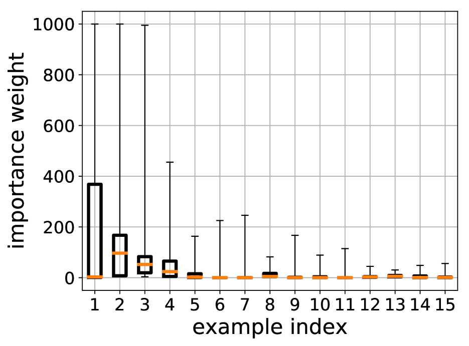
(a) $\mathcal{{M}}\rightarrow\mathcal{{S}}$ (ECE std. $5.60$)

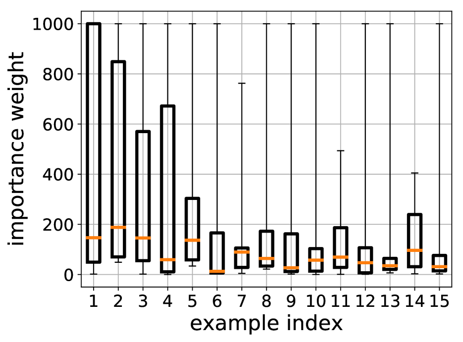
(b) $\mathcal{{M}}\rightarrow\mathcal{{U}}$ (ECE std. $1.45$)

Figure 2: These plots show the distribution of our importance weight estimates. For each source example, we estimate the importance weights on 10 runs. We choose 15 examples with the largest corresponding average estimated importance weight. For these 15 examples, we plot the median, minimum, and maximum of the estimated importance weights across the 10 runs.

ECE variance. Some of our benchmarks exhibit high variance ECEs—in particular, the benchmark MNIST to SVHN. Note that this variance is caused by randomness in our algorithm, since the randomness across runs is only based on different random choices by our algorithm. In particular, we believe the variance is caused by the variance in our learned source-discriminator $\hat{{g}}$, most likely due to optimization error when fitting $\bar{g}$ and $\psi$. This variance can cause our importance weights to vary drastically across runs. For example, Figure 2 shows the distribution of the estimated importance weights on the benchmarks MNIST to SVHN (which has high ECE variance) and MNIST to USPS (which has low ECE variance) over 10 runs. As can be seen, the the importance weights vary greatly across runs.

Interestingly, the variances appear to be larger on the shift from MNIST to USPS, even though the variance for the ECE on this benchmark is smaller. However, note that for the shift from MNIST to SVHN, the importance weights are close to zero for most examples. We believe that for the shift from MNIST to USPS, even if the importance weights have high variance, the noise is averaged out across many examples. In contrast, for SVHN, there are very few relevant examples; thus, if we obtain poor estimates of the importance weights for these relevant examples, then the subsequent calibration step will perform poorly.

7 Conclusion

We have proposed a novel approach for calibrated prediction in the presence of covariate shift, and empirically demonstrated that our approach outperforms existing ones. Future work includes handling the case of online covariate shift (i.e., the classifier is observing new examples sequentially), and extending our results beyond the classification setting.

Acknowledgements

This work was supported in part by NSF CCF-1910769 and by the Air Force Research Laboratory and the Defense Advanced Research Projects Agency under Contract No. FA8750-18-C-0090. Any opinions, findings and conclusions or recommendations expressed in this material are those of the author(s) and do not necessarily reflect the views of the Air Force Research Laboratory (AFRL), the Defense Advanced Research Projects Agency (DARPA), the Department of Defense, or the United States Government.

Appendix A Additional Results

A.1 Reliability Diagrams

The reliability diagram is an intuitive visualization of the empirical calibration error (ECE) in (11) (DeGroot and Fienberg, 1983; Niculescu-Mizil and Caruana, 2005). In particular, the diagram shows the averaged predicted uncertainty (i.e., $\frac{1}{|\mathcal{{T}}_{b}|}\sum_{(x,\mathbf{{y}})\in\mathcal{{T}}_{b}}\hat{{f}}(x)_{f(x)}$) on the $x$-axis, and the empirical accuracy (i.e., $\frac{1}{|\mathcal{{T}}_{b}|}\sum_{(x,\mathbf{{y}})\in\mathcal{{T}}_{b}}\mathbf{{y}}_{f(x)}$) on the $y$-axis. Thus, if bars in the reliability diagram aligns with the diagonal, the ECE of the forecaster in consideration is zero. If the bars are below the diagonal, then the forecaster is over-confident on its uncertainty predictions. Along with the accuracy and confidence plots, each bar is weighted by the fraction of examples in each bin $b$ (i.e., $\frac{|\mathcal{{T}}_{b}|}{|\mathcal{{T}}|}$), which is also reflected in the ECE in (11).

We compare the reliability diagram for the temperature scaling approach and for our approach in Figure 3, Figure 4, Figure 5, Figure 6, Figure 7, Figure 8, and Figure 9.

A.2 Running Time

As with existing approaches to calibrated prediction (Guo et al., 2017), our approach relies on a second phase of training to calibrate the predicted probabilities. We measure the overhead of our calibration step compared to the time used to train the indistinguishable feature map. The results are:

• $\mathcal{{M}}\rightarrow\mathcal{{M}}$: 7840.8589 sec. (our overhead) vs. 1324.9306 sec. (total)

• $\mathcal{{U}}\rightarrow\mathcal{{M}}$: 14939.4707 sec. (our overhead) vs. 1001.3495 sec. (total)

• $\mathcal{{M}}\rightarrow\mathcal{{U}}$: 16900.7378 sec. (our overhead) vs. 1217.413 sec. (total)

• $\mathcal{{S}}\rightarrow\mathcal{{M}}$: 16437.2544 sec. (our overhead) vs. 581.6673 sec. (total)

• $\mathcal{{M}}\rightarrow\mathcal{{S}}$: 4437.1197 sec. (our overhead) vs. 1460.2213 sec. (total)

• $\mathcal{{A}}\rightarrow\mathcal{{W}}$: 16068.9053 sec. (our overhead) vs. 907.5134 sec. (total)

• $\mathcal{{D}}\rightarrow\mathcal{{A}}$: 9576.0645 sec. (our overhead) vs. 9015.7301 sec. (total)

• $\mathcal{{W}}\rightarrow\mathcal{{A}}$: 18602.4316 sec. (our overhead) vs. 7217.6859 sec. (total)

In all but one case, the overhead from calibration is less than $1/4$ the total time taken (i.e., for both calibration and indistinguishable feature learning). This overhead is reasonable for obtaining calibrated probabilities.

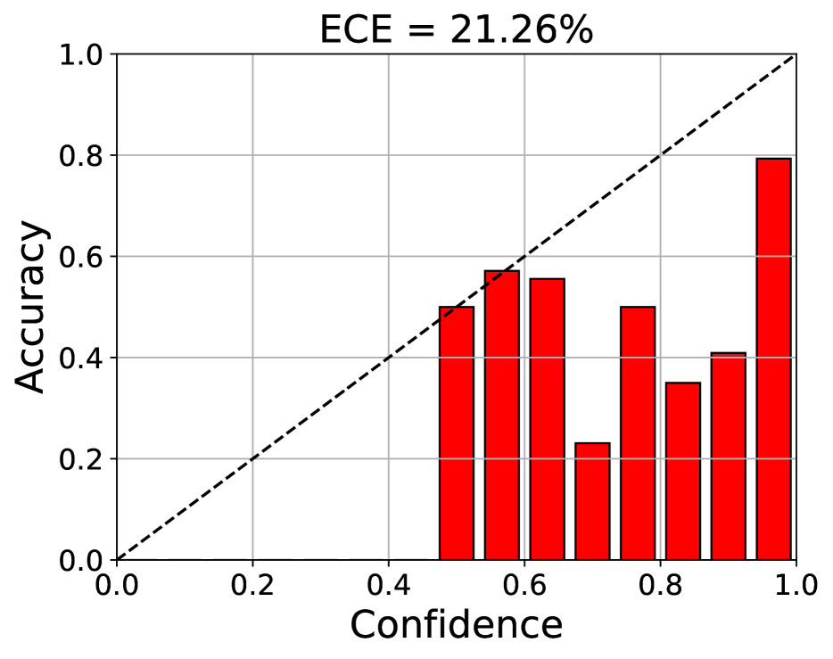
(a) None

(b) Temp. scaling

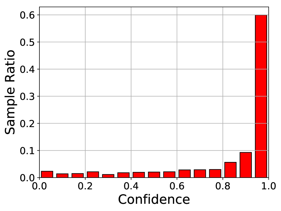
(c) Temp.+FL+IW

Figure 3: Reliability diagram of the shift $\mathcal{{M}}\rightarrow\mathcal{{U}}$ from one experiment among ten.

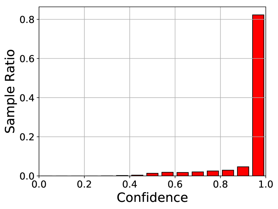
(a) None

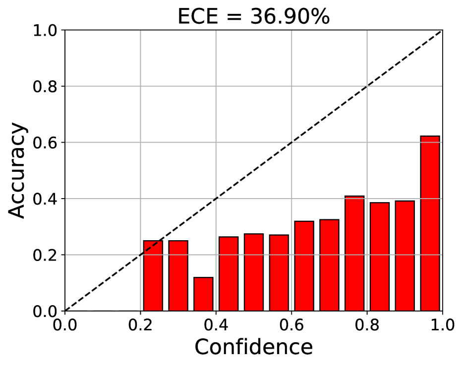
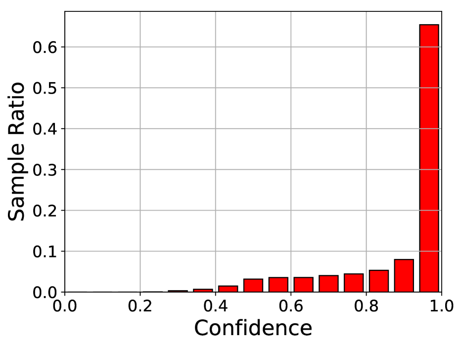
(b) Temp. scaling

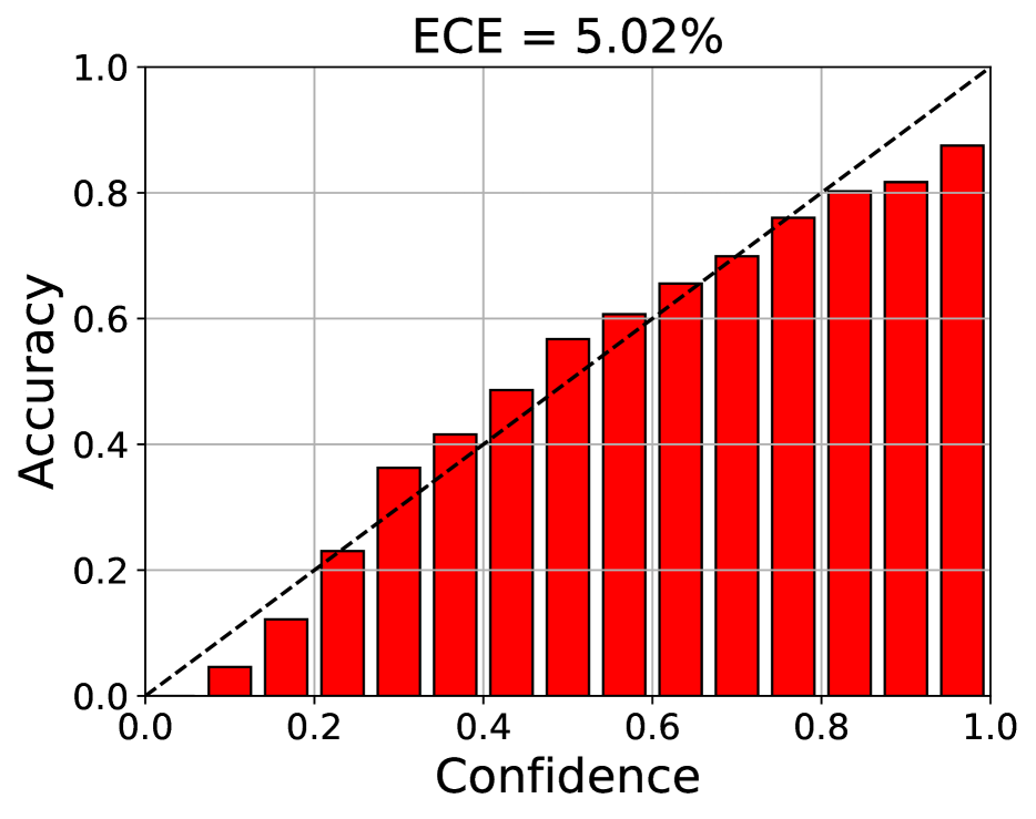
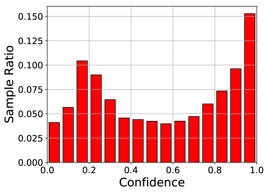
(c) Temp.+FL+IW

Figure 4: Reliability diagram of the shift $\mathcal{{U}}\rightarrow\mathcal{{M}}$ from one experiment among ten.

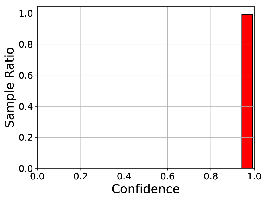
(a) None

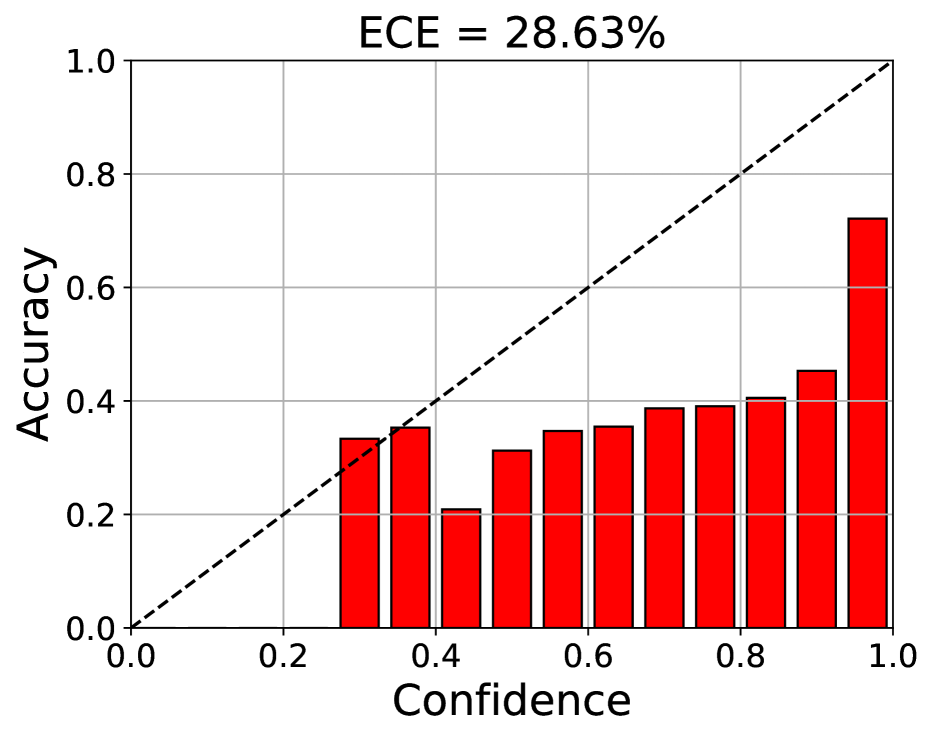
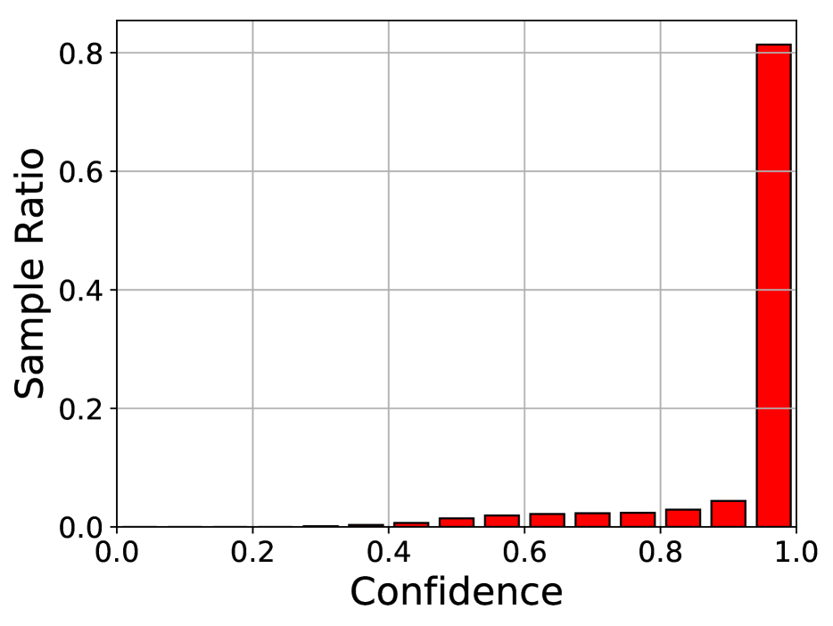
(b) Temp. scaling

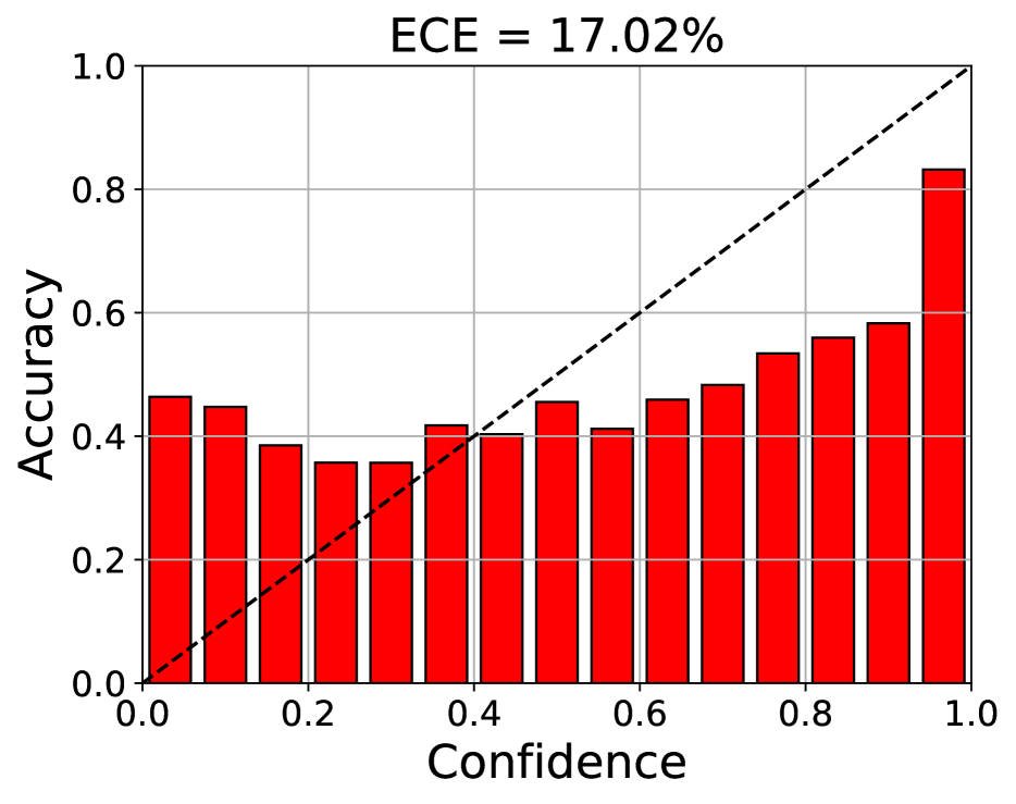
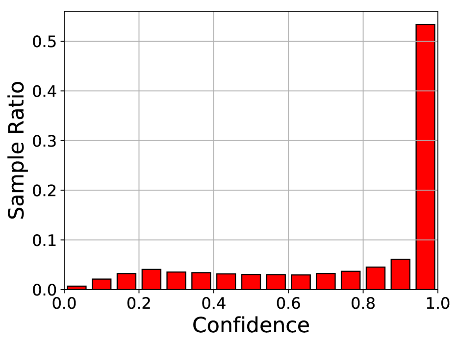
(c) Temp.+FL+IW

Figure 5: Reliability diagram of the shift $\mathcal{{S}}\rightarrow\mathcal{{M}}$ from one experiment among ten.

(a) None

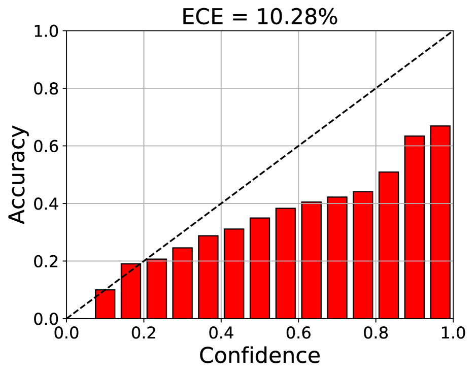
(b) Temp. scaling

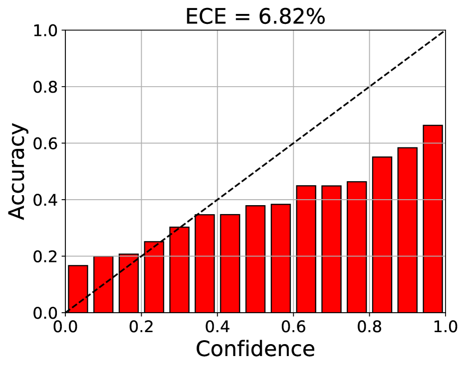
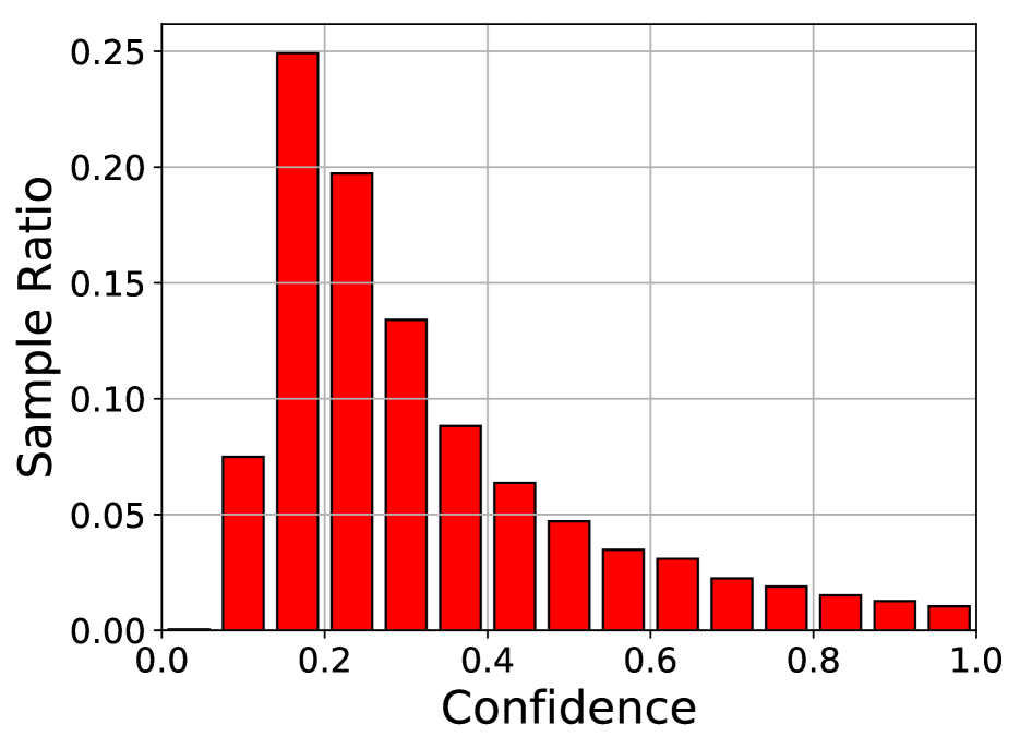
(c) Temp.+FL+IW

Figure 6: Reliability diagram of the shift $\mathcal{{M}}\rightarrow\mathcal{{S}}$ from one experiment among ten.

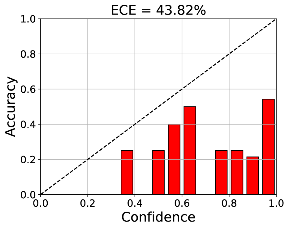
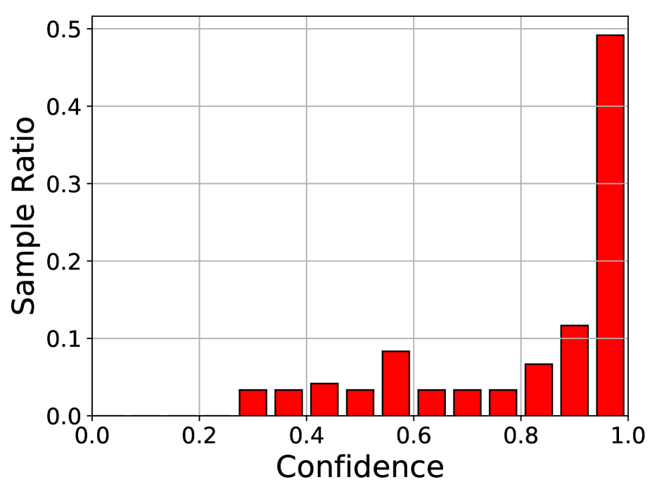
(a) None

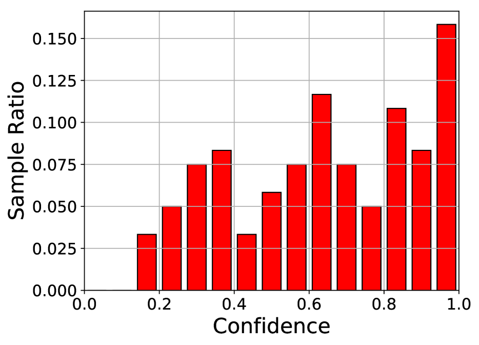
(b) Temp. scaling

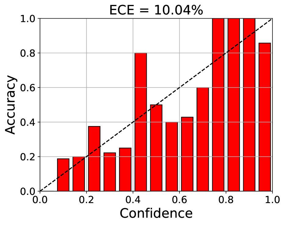
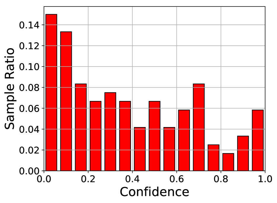
(c) Temp.+FL+IW

Figure 7: Reliability diagram of the shift $\mathcal{{A}}\rightarrow\mathcal{{W}}$ from one experiment among ten.

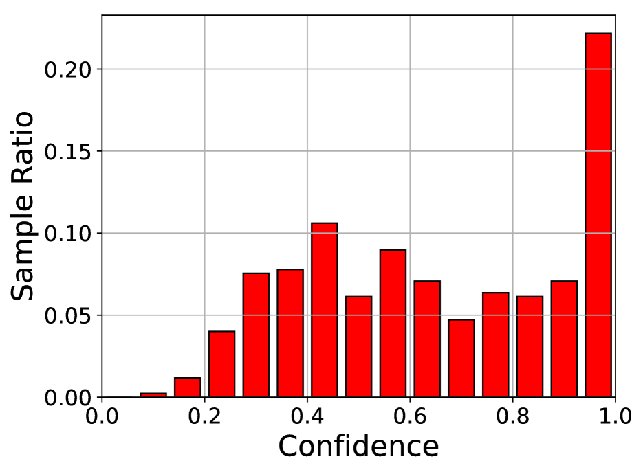
(a) None

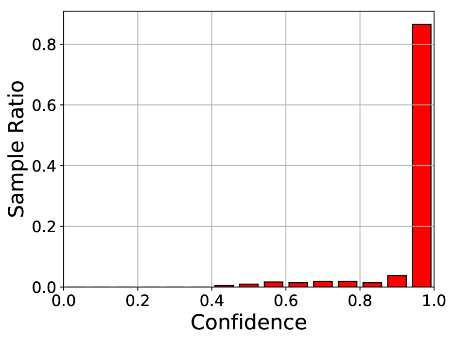
(b) Temp. scaling

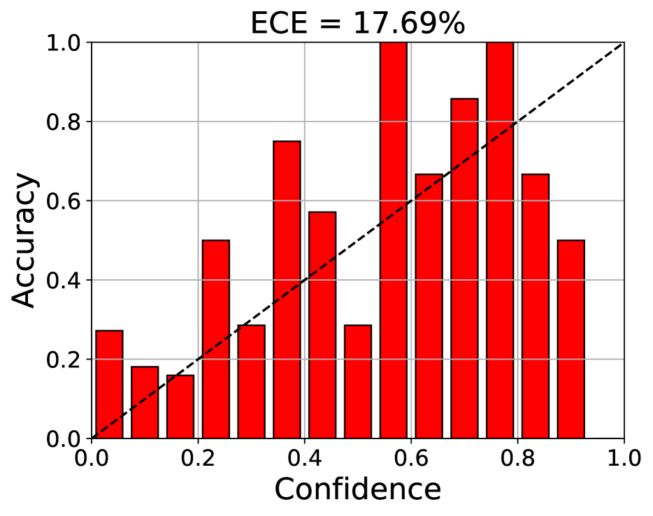
(c) Temp.+FL+IW

Figure 8: Reliability diagram of the shift $\mathcal{{D}}\rightarrow\mathcal{{A}}$ from one experiment among ten.

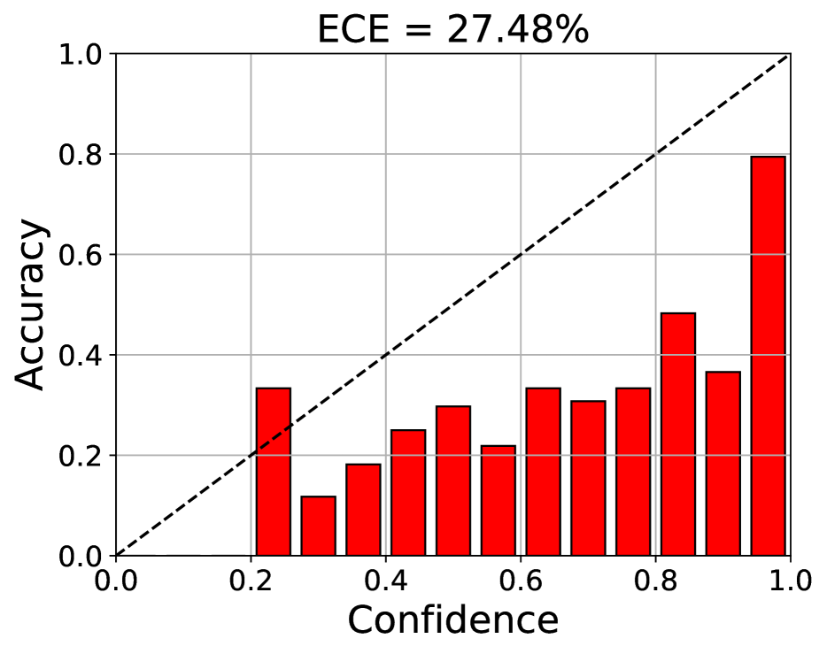
(a) None

(b) Temp. scaling

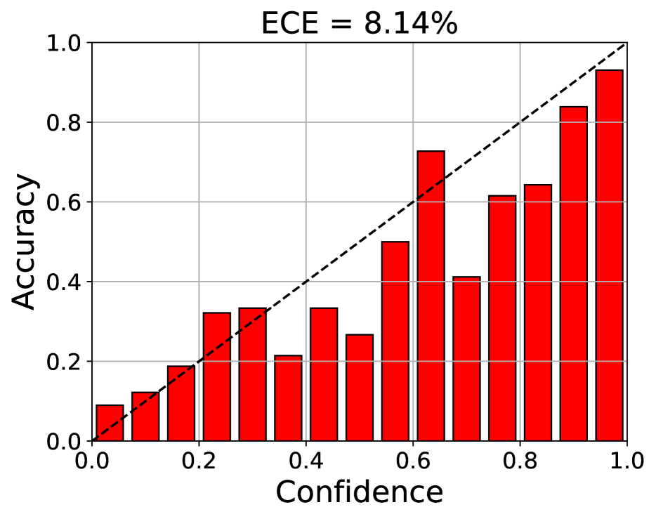
(c) Temp.+FL+IW

Figure 9: Reliability diagram of the shift $\mathcal{{W}}\rightarrow\mathcal{{A}}$ from one experiment among ten.

References

- Barber et al. (2019) R. F. Barber, E. J. Candes, A. Ramdas, and R. J. Tibshirani. Predictive inference with the jackknife+. arXiv preprint arXiv:1905.02928, 2019.
- Ben-David et al. (2007) S. Ben-David, J. Blitzer, K. Crammer, and F. Pereira. Analysis of representations for domain adaptation. In Advances in neural information processing systems, pages 137–144, 2007.
- Bickel et al. (2007) S. Bickel, M. Brückner, and T. Scheffer. Discriminative learning for differing training and test distributions. In Proceedings of the 24th international conference on Machine learning, pages 81–88. ACM, 2007.
- Brier (1950) G. W. Brier. Verification of forecasts expressed in terms of probability. Monthey Weather Review, 78(1):1–3, 1950.
- Cortes et al. (2008) C. Cortes, M. Mohri, M. Riley, and A. Rostamizadeh. Sample selection bias correction theory. In International conference on algorithmic learning theory, pages 38–53. Springer, 2008.
- Cortes et al. (2010) C. Cortes, Y. Mansour, and M. Mohri. Learning bounds for importance weighting. In Advances in neural information processing systems, pages 442–450, 2010.
- DeGroot and Fienberg (1983) M. H. DeGroot and S. E. Fienberg. The comparison and evaluation of forecasters. Journal of the Royal Statistical Society: Series D (The Statistician), 32(1-2):12–22, 1983.
- Ganin et al. (2016) Y. Ganin, E. Ustinova, H. Ajakan, P. Germain, H. Larochelle, F. Laviolette, M. Marchand, and V. Lempitsky. Domain-adversarial training of neural networks. Journal of Machine Learning Research, 17(59):1–35, 2016. URL http://jmlr.org/papers/v17/15-239.html.
- Guo et al. (2017) C. Guo, G. Pleiss, Y. Sun, and K. Q. Weinberger. On calibration of modern neural networks. arXiv preprint arXiv:1706.04599, 2017.
- Hoffman et al. (2017) J. Hoffman, E. Tzeng, T. Park, J.-Y. Zhu, P. Isola, K. Saenko, A. A. Efros, and T. Darrell. Cycada: Cycle-consistent adversarial domain adaptation. arXiv preprint arXiv:1711.03213, 2017.
- Huang et al. (2007) J. Huang, A. Gretton, K. Borgwardt, B. Schölkopf, and A. J. Smola. Correcting sample selection bias by unlabeled data. In Advances in neural information processing systems, pages 601–608, 2007.
- Hull (1994) J. J. Hull. A database for handwritten text recognition research. IEEE Transactions on pattern analysis and machine intelligence, 16(5):550–554, 1994.
- Kanamori et al. (2009) T. Kanamori, S. Hido, and M. Sugiyama. A least-squares approach to direct importance estimation. Journal of Machine Learning Research, 10(Jul):1391–1445, 2009.
- Kuleshov and Ermon (2017) V. Kuleshov and S. Ermon. Estimating uncertainty online against an adversary. In Thirty-First AAAI Conference on Artificial Intelligence, 2017.
- Kuleshov and Liang (2015) V. Kuleshov and P. S. Liang. Calibrated structured prediction. In Advances in Neural Information Processing Systems, pages 3474–3482, 2015.
- Kuleshov et al. (2018) V. Kuleshov, N. Fenner, and S. Ermon. Accurate uncertainties for deep learning using calibrated regression. arXiv preprint arXiv:1807.00263, 2018.
- LeCun et al. (1989) Y. LeCun, B. Boser, J. S. Denker, D. Henderson, R. E. Howard, W. Hubbard, and L. D. Jackel. Backpropagation applied to handwritten zip code recognition. Neural computation, 1(4):541–551, 1989.
- Long et al. (2017) M. Long, H. Zhu, J. Wang, and M. I. Jordan. Deep transfer learning with joint adaptation networks. In Proceedings of the 34th International Conference on Machine Learning-Volume 70, pages 2208–2217. JMLR. org, 2017.
- Long et al. (2018) M. Long, Z. Cao, J. Wang, and M. I. Jordan. Conditional adversarial domain adaptation. In Advances in Neural Information Processing Systems, pages 1640–1650, 2018.
- Murphy (1972) A. H. Murphy. Scalar and vector partitions of the probability score: Part i. two-state situation. Journal of Applied Meteorology, 11(2):273–282, 1972.
- Murphy and Winkler (1977) A. H. Murphy and R. L. Winkler. Reliability of subjective probability forecasts of precipitation and temperature. Journal of the Royal Statistical Society: Series C (Applied Statistics), 26(1):41–47, 1977.
- Naeini et al. (2015) M. P. Naeini, G. Cooper, and M. Hauskrecht. Obtaining well calibrated probabilities using bayesian binning. In Twenty-Ninth AAAI Conference on Artificial Intelligence, 2015.
- Netzer et al. (2011) Y. Netzer, T. Wang, A. Coates, A. Bissacco, B. Wu, and A. Y. Ng. Reading digits in natural images with unsupervised feature learning. In NIPS Workshop on Deep Learning and Unsupervised Feature Learning, 2011.
- Niculescu-Mizil and Caruana (2005) A. Niculescu-Mizil and R. Caruana. Predicting good probabilities with supervised learning. In Proceedings of the 22nd international conference on Machine learning, pages 625–632. ACM, 2005.
- Papadopoulos (2008) H. Papadopoulos. Inductive conformal prediction: Theory and application to neural networks. In Tools in artificial intelligence. IntechOpen, 2008.
- Park et al. (2020) S. Park, O. Bastani, N. Matni, and I. Lee. PAC confidence sets for deep neural networks via calibrated prediction. In International Conference on Learning Representations, 2020. URL https://openreview.net/forum?id=BJxVI04YvB.
- Platt et al. (1999) J. Platt et al. Probabilistic outputs for support vector machines and comparisons to regularized likelihood methods. Advances in large margin classifiers, 1999.
- Saenko et al. (2010) K. Saenko, B. Kulis, M. Fritz, and T. Darrell. Adapting visual category models to new domains. In European conference on computer vision, pages 213–226. Springer, 2010.
- Sankaranarayanan et al. (2018) S. Sankaranarayanan, Y. Balaji, C. D. Castillo, and R. Chellappa. Generate to adapt: Aligning domains using generative adversarial networks. In Proceedings of the IEEE Conference on Computer Vision and Pattern Recognition, pages 8503–8512, 2018.
- Shimodaira (2000) H. Shimodaira. Improving predictive inference under covariate shift by weighting the log-likelihood function. Journal of statistical planning and inference, 90(2):227–244, 2000.
- Snoek et al. (2019) J. Snoek, Y. Ovadia, E. Fertig, B. Lakshminarayanan, S. Nowozin, D. Sculley, J. Dillon, J. Ren, and Z. Nado. Can you trust your model’s uncertainty? evaluating predictive uncertainty under dataset shift. In Advances in Neural Information Processing Systems, pages 13969–13980, 2019.
- Sugiyama et al. (2007) M. Sugiyama, M. Krauledat, and K.-R. Muller. Covariate shift adaptation by importance weighted cross validation. Journal of Machine Learning Research, 8(May):985–1005, 2007.
- Sugiyama et al. (2008) M. Sugiyama, S. Nakajima, H. Kashima, P. V. Buenau, and M. Kawanabe. Direct importance estimation with model selection and its application to covariate shift adaptation. In Advances in neural information processing systems, pages 1433–1440, 2008.
- Vapnik (1995) V. N. Vapnik. The Nature of Statistical Learning Theory. Springer-Verlag New York, Inc., 1995.
- Vovk (2013) V. Vovk. Conditional validity of inductive conformal predictors. Machine learning, 92(2-3):349–376, 2013.
- Zadrozny and Elkan (2001) B. Zadrozny and C. Elkan. Obtaining calibrated probability estimates from decision trees and naive bayesian classifiers. In In Proceedings of the Eighteenth International Conference on Machine Learning. Citeseer, 2001.
- Zadrozny and Elkan (2002) B. Zadrozny and C. Elkan. Transforming classifier scores into accurate multiclass probability estimates. In Proceedings of the eighth ACM SIGKDD international conference on Knowledge discovery and data mining, pages 694–699. ACM, 2002.