OpEn: Code Generation for Embedded Nonconvex Optimization

Pantelis Sopasakis    Emil Fresk    Panagiotis Patrinos Queen’s University Belfast, School of Electronics, Electrical Engineering and Computer Science (EEECS) and Centre for Intelligent and Autonomous Manufacturing Systems (i-AMS), Ashby Building, Stranmillis Road, BT9 5AG Belfast, Northern Ireland WideFind AB, Aurorum 1C, 977 75 Luleå, Sweden KU Leuven, Department of Electrical Engineering (ESAT), STADIUS Center for Dynamical Systems, Signal Processing and Data Analytics & Optimization in Engineering (OPTEC), Kasteelpark Arenberg 10, 3001 Leuven, Belgium.
Abstract

We present Optimization Engine (OpEn): an open-source code generation tool for real-time embedded nonconvex optimization, which implements a novel numerical method. OpEn combines the proximal averaged Newton-type method for optimal control (PANOC) with the penalty and augmented Lagrangian methods to compute approximate stationary points of nonconvex problems. The proposed method involves very simple algebraic operations such as vector products, has a low memory footprint and exhibits very good convergence properties that allow the solution of nonconvex problems on embedded devices. OpEn’s core solver is written is Rust — a modern, high-performance, memory-safe and thread-safe systems programming language — while users can call it from Python, MATLAB, C, C++ or over a TCP socket.

keywords:
Embedded numerical optimization; nonconvex optimization problems; code genera- tion; model predictive control; moving horizon estimation
thanks: The work of P. Patrinos was supported by: FWO projects: No. G086318N; No. G086518N; Fonds de la Recherche Scientifique – FNRS, the Fonds Wetenschappelijk Onderzoek – Vlaanderen under EOS Project No. 30468160 (SeLMA), Research Council KU Leuven C1 project No. C14/18/068 and the Ford–KU Leuven Research Alliance project. Corresponding author email: p.sopasakis@qub.ac.uk.

, and

1 Introduction

In embedded applications it is often necessary to solve optimization problems in real time. Typical examples involve moving horizon estimation, model predictive control and online learning (Ferreau et al., 2017). The distinctive features of embedded real time computing are the limited computing and storage capabilities of hardware devices, the presence of stringent runtime requirements, the increased need for memory safety and reliability, the need for simple numerical methods which can be verified easily, and the need for design paradigms that involve code generation.

A significant research effort has been dedicated to numerical optimization software with code generation capabilities for convex problems such as CVXGen (Mattingley and Boyd, 2012, 2010), SPLIT (Shukla et al., 2017), OSQP (Banjac et al., 2017), and μ𝜇\muAO-MPC (Zometa et al., 2013). Kouzoupis et al. (2015) provide benchmarks of numerical optimization methods for embedded quadratic programming.

Nonconvex optimization problems are typically solved with sequential convex programming (SCP) (Zillober et al., 2004) and interior point (IP) methods (Zanelli et al., 2017; Gopal and Biegler, 1998). Several software are available for nonconvex optimization such as SNOPT (Gill et al., 2005), Acado (Verschueren et al., 2018; Houska et al., 2011a, b) and IPOPT (Wächter and Biegler, 2006).

Nonetheless, SCP and IP methods have a high per-iteration computation cost and involve expensive operations such as the solution of quadratic programming problems or the solution of linear systems. Was it not for their slow convergence, first-order methods such as the projected gradient method, would be ideal for embedded applications. Stella et al. (2017) proposed the proximal averaged Newton-type method for optimal control (PANOC), which uses exactly the same oracle as the projected gradient method but exhibits superior convergence characteristics and has been found to outperform SCP and IP methods (Sathya et al., 2018; Small et al., 2019).

PANOC can solve problems with a smooth cost function and simple constraints on which one can compute projections. More general constraints can be relaxed and replaced by penalty functions (soft constraints). The penalty method can then be applied to obtain near-feasible solutions (Hermans et al., 2018). However, as the penalty parameter needs to grow unbounded, it is likely that it will overshadow the cost function and lead to highly ill conditioned problems. In this paper we propose a numerical method to determine stationary points of constrained nonconvex optimization problems by combining the penalty and the augmented Lagrangian methods. Moreover, we present OpEn: an open-source software an open-source code generation tool for real-time embedded nonconvex optimization with guaranteed safe memory management. In Section 5 we present two simulation examples – a model predictive controller for obstacle avoidance and a constrained nonlinear estimator – and provide comparisons with IPOPT and scipy’s SQP solver.

Preliminaries and Notation

We define INN={0,1,,N}subscriptIN𝑁01𝑁{\rm I\mathchoice{}{}{}{}N}_{N}=\{0,1,\ldots,N\}. We denote the set of extended-real numbers by IR¯=IR{}¯IRIR\overline{{\rm I\mathchoice{}{}{}{}R}}={\rm I\mathchoice{}{}{}{}R}\cup\{\infty\}. The Jacobian of a mapping F:IRmIRn:𝐹superscriptIR𝑚superscriptIR𝑛F:{\rm I\mathchoice{}{}{}{}R}^{m}\to{\rm I\mathchoice{}{}{}{}R}^{n} is denoted by JF𝐽𝐹JF. For two vectors, x,xIRn𝑥superscript𝑥superscriptIR𝑛x,x^{\prime}\in{\rm I\mathchoice{}{}{}{}R}^{n}, the relation xx𝑥superscript𝑥x\leq x^{\prime} is meant in the pointwise sense. For xIR𝑥IRx\in{\rm I\mathchoice{}{}{}{}R}, we define [x]+=max{0,x}subscriptdelimited-[]𝑥0𝑥\left[{}x{}\right]_{\scriptscriptstyle+}=\max\{0,x\} and for xIRn𝑥superscriptIR𝑛x\in{\rm I\mathchoice{}{}{}{}R}^{n}, [x]+subscriptdelimited-[]𝑥\left[{}x{}\right]_{\scriptscriptstyle+} is defined element wise. The projection of a vector xIRn𝑥superscriptIR𝑛x\in{\rm I\mathchoice{}{}{}{}R}^{n} on a nonempty, closed, convex set CIRn𝐶superscriptIR𝑛C\subseteq{\rm I\mathchoice{}{}{}{}R}^{n} is defined as ΠC(x)=argminyCyxsubscriptΠ𝐶𝑥subscriptargmin𝑦𝐶norm𝑦𝑥\operatorname{\Pi}_{C}(x)=\operatorname*{argmin}_{y\in C}\|y-x\| and the distance of xIRn𝑥superscriptIR𝑛x\in{\rm I\mathchoice{}{}{}{}R}^{n} from C𝐶C is defined as distC(x)=minyCyxsubscriptdist𝐶𝑥subscript𝑦𝐶norm𝑦𝑥\operatorname{dist}_{C}(x)=\min_{y\in C}\|y-x\|. The support function of a nonempty, closed, convex set CIRn𝐶superscriptIR𝑛C\subseteq{\rm I\mathchoice{}{}{}{}R}^{n} is a function δC:IRnIR¯:superscriptsubscript𝛿𝐶superscriptIR𝑛¯IR\delta_{C}^{*}:{\rm I\mathchoice{}{}{}{}R}^{n}\to\overline{{\rm I\mathchoice{}{}{}{}R}} defined as δC(y)=supxCyxsuperscriptsubscript𝛿𝐶𝑦subscriptsupremum𝑥𝐶superscript𝑦top𝑥\delta_{C}^{*}(y)=\sup_{x\in C}y^{\top}x. For a cone KIRn𝐾superscriptIR𝑛K\subseteq{\rm I\mathchoice{}{}{}{}R}^{n}, we define its polar to be the cone K={yIRn:yx0}superscript𝐾conditional-set𝑦superscriptIR𝑛superscript𝑦top𝑥0K^{\circ}=\{y\in{\rm I\mathchoice{}{}{}{}R}^{n}{}:{}y^{\top}x\leq 0\}. The normal cone of a set CIRn𝐶superscriptIR𝑛C\subseteq{\rm I\mathchoice{}{}{}{}R}^{n} is defined as that subdifferential of δCsubscript𝛿𝐶\delta_{C}, that is, NC(x)=δC(x)subscript𝑁𝐶𝑥subscript𝛿𝐶𝑥N_{C}(x)=\partial\delta_{C}(x), for xIRn𝑥superscriptIR𝑛x\in{\rm I\mathchoice{}{}{}{}R}^{n}.

2 Problem statement

Consider the following parametric optimization problem

(p):minimizeuU:𝑝subscriptminimize𝑢𝑈\displaystyle\mathbb{P}(p){}:{}\operatorname*{minimize}_{u{}\in{}U}\, f(u,p),𝑓𝑢𝑝\displaystyle f(u,p), (1a)
subj.to:\displaystyle\operatorname{subj.\,to:}\, F1(u,p)C,subscript𝐹1𝑢𝑝𝐶\displaystyle F_{1}(u,p)\in C, (1b)
F2(u,p)=0,subscript𝐹2𝑢𝑝0\displaystyle F_{2}(u,p)=0, (1c)

where for each pIRnp𝑝superscriptIRsubscript𝑛𝑝p\in{\rm I\mathchoice{}{}{}{}R}^{n_{p}}, f(,p):IRnIR:𝑓𝑝superscriptIR𝑛IRf({}\cdot{},p):{\rm I\mathchoice{}{}{}{}R}^{n}\to{\rm I\mathchoice{}{}{}{}R} is a (possibly nonconvex) continuously differentiable function with Lfsubscript𝐿𝑓L_{f}-Lipschitz gradient and UIRn𝑈superscriptIR𝑛U\subseteq{\rm I\mathchoice{}{}{}{}R}^{n} is a nonempty, closed — but not necessarily convex — set such that we can compute projections on it. Moreover, F1(,p):IRnIRn1:subscript𝐹1𝑝superscriptIR𝑛superscriptIRsubscript𝑛1F_{1}({}\cdot{},p):{\rm I\mathchoice{}{}{}{}R}^{n}\to{\rm I\mathchoice{}{}{}{}R}^{n_{1}} is a smooth mapping with Lipschitz-continuous Jacobian which is bounded on U𝑈U. Set CIRn1𝐶superscriptIRsubscript𝑛1C\subseteq{\rm I\mathchoice{}{}{}{}R}^{n_{1}} is a convex set from which we can compute distances. Mapping F2(,p):IRnIRn2:subscript𝐹2𝑝superscriptIR𝑛superscriptIRsubscript𝑛2F_{2}({\cdot},p):{\rm I\mathchoice{}{}{}{}R}^{n}\to{\rm I\mathchoice{}{}{}{}R}^{n_{2}} is such that F2(;p)2superscriptnormsubscript𝐹2𝑝2\|F_{2}({}\cdot{};p)\|^{2} is a continuously differentiable function with Lipschitz-continuous gradient.

In particular, constraints (1b) will be treated using the proposed augmented Lagrangian method, while constraints (1c) will be accounted for using the penalty method as we shall discuss in Section 3. Constraints of both types can be present at the same time.

Constraints (1c) can accommodate multiple vertical complementarity constraints (Scheel and Scholtes, 2000; Izmailov et al., 2012) of the form

i=1m[hi(u,p)]+=0,superscriptsubscriptproduct𝑖1𝑚subscriptdelimited-[]subscript𝑖𝑢𝑝0\prod_{i=1}^{m}\left[{}h_{i}(u,p){}\right]_{\scriptscriptstyle+}{}={}0, (2)

a special case of which arises in collision avoidance problems (Hermans et al., 2018; Sathya et al., 2018; Small et al., 2019). Such constraints do not satisfy the smoothness conditions, so they cannot be described in terms of the ALM-type constraints in (1b).

Set U𝑈U can be a Euclidean ball of radius r𝑟r centered at a point ucsubscript𝑢𝑐u_{c}, 2(uc,r)={uIRn:uuc2r}subscript2subscript𝑢𝑐𝑟conditional-set𝑢superscriptIR𝑛subscriptnorm𝑢subscript𝑢𝑐2𝑟\mathcal{B}_{2}(u_{c},r)=\{u\in{\rm I\mathchoice{}{}{}{}R}^{n}{}:{}\|u-u_{c}\|_{2}\leq r\}, an infinity ball, (uc,r)={uIRn:uucr}subscriptsubscript𝑢𝑐𝑟conditional-set𝑢superscriptIR𝑛subscriptnorm𝑢subscript𝑢𝑐𝑟\mathcal{B}_{\infty}(u_{c},r)=\{u\in{\rm I\mathchoice{}{}{}{}R}^{n}{}:{}\|u-u_{c}\|_{\infty}\leq r\}, a rectangle, {uIRn:uminuumax}conditional-set𝑢superscriptIR𝑛subscript𝑢min𝑢subscript𝑢max\{u\in{\rm I\mathchoice{}{}{}{}R}^{n}{}:{}u_{\mathrm{min}}\leq u\leq u_{\mathrm{max}}\} (where some coordinates of uminsubscript𝑢minu_{\mathrm{min}} and umaxsubscript𝑢maxu_{\mathrm{max}} are allowed to be equal to -\infty and \infty respectively), a finite set {u(1),u(2),,u(q)}superscript𝑢1superscript𝑢2superscript𝑢𝑞\{u^{(1)},u^{(2)},\ldots,u^{(q)}\}, or a Cartesian product of any such sets.

The above formulation can accommodate equality constraints, either through constraint (1c), or by using C={0}𝐶0C=\{0\}. It can also accommodate inequality constraints of the general form

H(u,p)0,𝐻𝑢𝑝0H(u,p)\leq 0, (3)

by using either F1(u,p)=H(u,p)subscript𝐹1𝑢𝑝𝐻𝑢𝑝F_{1}(u,p)=H(u,p) and C={vIRn1:v0}𝐶conditional-set𝑣superscriptIRsubscript𝑛1𝑣0C{}={}\{v\in{\rm I\mathchoice{}{}{}{}R}^{n_{1}}{}:{}v\leq 0\}, or F2(u,p)=[H(u,p)]+subscript𝐹2𝑢𝑝subscriptdelimited-[]𝐻𝑢𝑝F_{2}(u,p){}={}\left[{}{}H(u,p){}{}\right]_{\scriptscriptstyle+}. Furthermore, constraint (1b) allow the designer to encode norm bounds using C=2(uc,r)𝐶subscript2subscript𝑢𝑐𝑟C=\mathcal{B}_{2}(u_{c},r) or C=(uc,r)𝐶subscriptsubscript𝑢𝑐𝑟C=\mathcal{B}_{\infty}(u_{c},r), or constraints involving second-order cones, C=SOCαn1{u=(x,t),xIRn11,tIR:xαt}𝐶superscriptsubscriptSOC𝛼subscript𝑛1conditional-setformulae-sequence𝑢𝑥𝑡formulae-sequence𝑥superscriptIRsubscript𝑛11𝑡IRnorm𝑥𝛼𝑡C{}={}\mathrm{SOC}_{\alpha}^{n_{1}}{}\coloneqq{}\{u=(x,t),x\in{\rm I\mathchoice{}{}{}{}R}^{n_{1}-1},t\in{\rm I\mathchoice{}{}{}{}R}:\|x\|\leq\alpha t\}, for some α>0𝛼0\alpha>0.

Optimal control and estimation problems can be written in the form of Problem (1) in a number of different ways. For instance, consider the following discrete-time optimal control problem

(x0):minimize:subscript𝑥0minimize\displaystyle\mathbb{P}(x_{0}):\operatorname*{minimize}\, N(xN)+t=0N1t(xt,ut)subscript𝑁subscript𝑥𝑁superscriptsubscript𝑡0𝑁1subscript𝑡subscript𝑥𝑡subscript𝑢𝑡\displaystyle\ell_{N}(x_{N})+\sum_{t=0}^{N-1}\ell_{t}(x_{t},u_{t}) (4a)
subj.to:\displaystyle\operatorname{subj.\,to:}\, utUt,subscript𝑢𝑡subscript𝑈𝑡\displaystyle u_{t}\in U_{t}, (4b)
xt+1=Φt(xt,ut),subscript𝑥𝑡1subscriptΦ𝑡subscript𝑥𝑡subscript𝑢𝑡\displaystyle x_{t+1}=\Phi_{t}(x_{t},u_{t}), (4c)
Ht(xt,ut)0,subscript𝐻𝑡subscript𝑥𝑡subscript𝑢𝑡0\displaystyle H_{t}(x_{t},u_{t})\leq 0, (4d)
HN(xN)0,subscript𝐻𝑁subscript𝑥𝑁0\displaystyle H_{N}(x_{N})\leq 0, (4e)

for tINN1𝑡subscriptIN𝑁1t\in{\rm I\mathchoice{}{}{}{}N}_{N-1}, where Utsubscript𝑈𝑡U_{t} are sets on which one can easily compute projections. One may follow the single shooting approach, in which the minimization is carried out over the sequence of control actions, u=(u0,,uN1)𝑢subscript𝑢0subscript𝑢𝑁1u=(u_{0},\ldots,u_{N-1}), and the sequence of states is eliminated by defining a sequence of function F0(u,x0)=x0subscript𝐹0𝑢subscript𝑥0subscript𝑥0F_{0}(u,x_{0})=x_{0} and Ft+1(u,x0)=Φt(Ft(u,x0),ut)subscript𝐹𝑡1𝑢subscript𝑥0subscriptΦ𝑡subscript𝐹𝑡𝑢subscript𝑥0subscript𝑢𝑡F_{t+1}(u,x_{0})=\Phi_{t}(F_{t}(u,x_{0}),u_{t}) for tINN1𝑡subscriptIN𝑁1t\in{\rm I\mathchoice{}{}{}{}N}_{N-1}. We may then define the cost function

f(u,x0)=N(FN(u,x0))+t=0N1t(Ft(u,x0),ut).𝑓𝑢subscript𝑥0subscript𝑁subscript𝐹𝑁𝑢subscript𝑥0superscriptsubscript𝑡0𝑁1subscript𝑡subscript𝐹𝑡𝑢subscript𝑥0subscript𝑢𝑡f(u,x_{0})=\ell_{N}(F_{N}(u,x_{0}))+\sum_{t=0}^{N-1}\ell_{t}(F_{t}(u,x_{0}),u_{t}). (5)

A second alternative is to follow the multiple shooting approach where the minimization is carried out over u=(u0,,uN1,x1,,xN)𝑢subscript𝑢0subscript𝑢𝑁1subscript𝑥1subscript𝑥𝑁u=(u_{0},\ldots,u_{N-1},x_{1},\ldots,x_{N}) and the system dynamics in Equation (4c) are treated as constraints.

Joint state-input constraints of the form (4d) and terminal constraints of the form (4e) can be cast using either F1subscript𝐹1F_{1} or F2subscript𝐹2F_{2} as discussed above.

3 Numerical algorithm

3.1 Augmented Lagrangian and Penalty Methods

In order to solve the original optimization problem, we shall use the augmented Lagrangian method (Birgin and Martínez, 2014). Hereafter, we shall drop the parameter p𝑝p for the sake of simplicity. We introduce the augmented Lagrangian function

Lc(u,v,y)f(u)+y,F1(u)v+c2F1(u)v2+c2F2(u)2,subscript𝐿𝑐𝑢𝑣𝑦𝑓𝑢𝑦subscript𝐹1𝑢𝑣𝑐2superscriptdelimited-∥∥subscript𝐹1𝑢𝑣2𝑐2superscriptdelimited-∥∥subscript𝐹2𝑢2L_{c}(u,v,y)\coloneqq f(u)+\langle y,F_{1}(u)-v\rangle\\ +\tfrac{c}{2}\|F_{1}(u)-v\|^{2}+\tfrac{c}{2}\|F_{2}(u)\|^{2}, (6)

defined for uU𝑢𝑈u\in U and vC𝑣𝐶v\in C, where c>0𝑐0c>0 is a constant penalty parameter and yIRn1𝑦superscriptIRsubscript𝑛1y\in{\rm I\mathchoice{}{}{}{}R}^{n_{1}} is the vector of Lagrange multipliers for constraints (1b). We can then show that

Proposition 1

The following holds for all yIRn1𝑦superscriptIRsubscript𝑛1y\in{\rm I\mathchoice{}{}{}{}R}^{n_{1}} and c>0𝑐0c>0

minuU,vCLc(u,v,y)=12cy2+minuUψ(u;c,y),subscriptformulae-sequence𝑢𝑈𝑣𝐶subscript𝐿𝑐𝑢𝑣𝑦12𝑐superscriptdelimited-∥∥𝑦2subscript𝑢𝑈𝜓𝑢𝑐𝑦\min_{u\in U,v\in C}L_{c}(u,v,y)=-\tfrac{1}{2c}\|y\|^{2}+\min_{u\in U}\psi(u;c,y), (7)

where

ψ(u;c,y)f(u)+c2[distC2(F1(u)+1cy)+F2(u)2].𝜓𝑢𝑐𝑦𝑓𝑢𝑐2delimited-[]superscriptsubscriptdist𝐶2subscript𝐹1𝑢1𝑐𝑦superscriptnormsubscript𝐹2𝑢2\psi(u;c,y){\coloneqq}f(u)\,{+}\,\tfrac{c}{2}\Big{[}\operatorname{dist}_{C}^{2}(F_{1}(u){+}\tfrac{1}{c}y)\,{+}\,\|F_{2}(u)\|^{2}\Big{]}\!\,. (8)
{pf}

For uU𝑢𝑈u{}\in{}U and vC𝑣𝐶v{}\in{}C, we have that

y,F1(u)v+c2F1(u)v2𝑦subscript𝐹1𝑢𝑣𝑐2superscriptnormsubscript𝐹1𝑢𝑣2\displaystyle{}\langle y,F_{1}(u)-v\rangle+\tfrac{c}{2}\|F_{1}(u)-v\|^{2}
=\displaystyle{}={} c1cy,F1(u)v+c2F1(u)v2+12cy212cy2𝑐1𝑐𝑦subscript𝐹1𝑢𝑣𝑐2superscriptnormsubscript𝐹1𝑢𝑣212𝑐superscriptnorm𝑦212𝑐superscriptnorm𝑦2\displaystyle c\langle\tfrac{1}{c}y,F_{1}(u){-}v\rangle+\tfrac{c}{2}\|F_{1}(u){-}v\|^{2}+\tfrac{1}{2c}\|y\|^{2}-\tfrac{1}{2c}\|y\|^{2}
=\displaystyle{}={} c2F1(u)v+1cy212cy2,𝑐2superscriptnormsubscript𝐹1𝑢𝑣1𝑐𝑦212𝑐superscriptnorm𝑦2\displaystyle\tfrac{c}{2}\|F_{1}(u)-v+\tfrac{1}{c}y\|^{2}-\tfrac{1}{2c}\|y\|^{2},

therefore,

minuU,vCLc(u,v,y)=12cy2+minuU{f(u)+c2F2(u)2+minvCc2F1(u)v+1cy2distC2(F1(u)+c1y)},subscriptformulae-sequence𝑢𝑈𝑣𝐶subscript𝐿𝑐𝑢𝑣𝑦12𝑐superscriptdelimited-∥∥𝑦2subscript𝑢𝑈𝑓𝑢𝑐2superscriptdelimited-∥∥subscript𝐹2𝑢2subscriptsubscript𝑣𝐶𝑐2superscriptnormsubscript𝐹1𝑢𝑣1𝑐𝑦2superscriptsubscriptdist𝐶2subscript𝐹1𝑢superscript𝑐1𝑦\min_{u\in U,v\in C}L_{c}(u,v,y)=-\tfrac{1}{2c}\|y\|^{2}+\min_{u\in U}\Big{\{}f(u)\\ +\tfrac{c}{2}\|F_{2}(u)\|^{2}+\vphantom{\min_{v\in C}\tfrac{c}{2}\|F_{1}(u)-v+\tfrac{1}{c}y\|^{2}}\smash{\underbracket{\min_{v\in C}\tfrac{c}{2}\|F_{1}(u)-v+\tfrac{1}{c}y\|^{2}}_{\operatorname{dist}_{C}^{2}(F_{1}(u)+c^{-1}y)}}\Big{\}}, (9)

which proves the assertion.  \Box

The above choice of an augmented Lagrangian function leads to Algorithm 1 where the inner problem takes the form

in(c,y):minimizeuUψ(u;c,y).:subscriptin𝑐𝑦subscriptminimize𝑢𝑈𝜓𝑢𝑐𝑦\mathbb{P}_{\mathrm{in}}(c,y){}:{}\operatorname*{minimize}_{u\in U}\psi(u;c,y). (10)

This problem has a smooth cost function and simple constraints, therefore, it can be solved using PANOC as we discuss in Section 3.2. The algorithm updates both a penalty parameter, c𝑐c, as well as a vector of Lagrange multipliers, yIRn1𝑦superscriptIRsubscript𝑛1y\in{\rm I\mathchoice{}{}{}{}R}^{n_{1}}, corresponding to constraint (1b) according to

yν+1=y¯ν+cν(F1(uν+1)ΠC(F1(uν+1)+cν1y¯ν)).superscript𝑦𝜈1superscript¯𝑦𝜈subscript𝑐𝜈subscript𝐹1superscript𝑢𝜈1subscriptΠ𝐶subscript𝐹1superscript𝑢𝜈1subscriptsuperscript𝑐1𝜈superscript¯𝑦𝜈y^{\nu+1}{}={}\bar{y}^{\nu}+c_{\nu}(F_{1}(u^{\nu+1})-\operatorname{\Pi}_{C}(F_{1}(u^{\nu+1})+c^{-1}_{\nu}\bar{y}^{\nu})). (11)
Algorithm 1 Augmented Lagrangian and penalty method
1:u0IRnusuperscript𝑢0superscriptIRsubscript𝑛𝑢u^{0}\in{\rm I\mathchoice{}{}{}{}R}^{n_{u}} (initial guess), pIRnp𝑝superscriptIRsubscript𝑛𝑝p\in{\rm I\mathchoice{}{}{}{}R}^{n_{p}} (parameter), y0IRn1superscript𝑦0superscriptIRsubscript𝑛1y^{0}\in{\rm I\mathchoice{}{}{}{}R}^{n_{1}} (initial guess for the Lagrange multipliers), ϵ,δ>0italic-ϵ𝛿0\epsilon,\delta>0 (tolerances), β𝛽\beta (tolerance decrease coefficient), ρ𝜌\rho (penalty update coefficient), θ𝜃\theta (sufficient decrease coefficient), YdomδC𝑌domsubscriptsuperscript𝛿𝐶Y\subseteq\operatorname{dom}\delta^{*}_{C} (compact set)
2:(ϵ,δ)italic-ϵ𝛿(\epsilon,\delta)-approximate solution (u,y)superscript𝑢superscript𝑦(u^{\star},y^{\star})
3:ϵ¯0=ϵ0subscript¯italic-ϵ0subscriptitalic-ϵ0\bar{\epsilon}_{0}=\epsilon_{0}
4:for ν=0,,νmax𝜈0subscript𝜈max\nu=0,\ldots,\nu_{\mathrm{max}} do
5:     y¯ν=ΠY(yν)superscript¯𝑦𝜈subscriptΠ𝑌superscript𝑦𝜈\bar{y}^{\nu}{}={}\operatorname{\Pi}_{Y}(y^{\nu})
6:     uν+1superscript𝑢𝜈1u^{\nu+1} is a solution of in(cν,y¯ν)subscriptinsubscript𝑐𝜈superscript¯𝑦𝜈\mathbb{P}_{\mathrm{in}}(c_{\nu},\bar{y}^{\nu}) with tolerance ϵ¯¯italic-ϵ\bar{\epsilon} and initial guess uνsuperscript𝑢𝜈u^{\nu}, using Algorithm 2
7:     yν+1=y¯ν+cν(F1(uν+1)ΠC(F1(uν+1)+cν1y¯ν))superscript𝑦𝜈1superscript¯𝑦𝜈subscript𝑐𝜈subscript𝐹1superscript𝑢𝜈1subscriptΠ𝐶subscript𝐹1superscript𝑢𝜈1subscriptsuperscript𝑐1𝜈superscript¯𝑦𝜈y^{\nu+1}{}={}\bar{y}^{\nu}+c_{\nu}(F_{1}(u^{\nu+1})-\operatorname{\Pi}_{C}(F_{1}(u^{\nu+1})+c^{-1}_{\nu}\bar{y}^{\nu}))
8:     zν+1=yν+1y¯νsubscript𝑧𝜈1subscriptnormsuperscript𝑦𝜈1superscript¯𝑦𝜈z_{\nu+1}{}={}\|y^{\nu+1}-\bar{y}^{\nu}\|_{\infty}, tν+1=F2(uν+1)subscript𝑡𝜈1subscriptnormsubscript𝐹2superscript𝑢𝜈1t_{\nu+1}=\|F_{2}(u^{\nu+1})\|_{\infty}
9:     if zν+1cνδsubscript𝑧𝜈1subscript𝑐𝜈𝛿z_{\nu+1}\leq c_{\nu}\delta, tν+1δsubscript𝑡𝜈1𝛿t_{\nu+1}\leq\delta and ϵ¯νϵsubscript¯italic-ϵ𝜈italic-ϵ\bar{\epsilon}_{\nu}\leq\epsilon then
10:         return (u,y)=(uν+1,yν+1)superscript𝑢superscript𝑦superscript𝑢𝜈1superscript𝑦𝜈1(u^{\star},y^{\star})=(u^{\nu+1},y^{\nu+1})
11:     else if ν>0𝜈0\nu>0, zν+1>θzνsubscript𝑧𝜈1𝜃subscript𝑧𝜈z_{\nu+1}>\theta z_{\nu}, tν+1>θtνsubscript𝑡𝜈1𝜃subscript𝑡𝜈t_{\nu+1}>\theta t_{\nu} then
12:         cν+1=ρcνsubscript𝑐𝜈1𝜌subscript𝑐𝜈c_{\nu+1}=\rho{}c_{\nu}      
13:     ϵ¯ν+1=βϵ¯νsubscript¯italic-ϵ𝜈1𝛽subscript¯italic-ϵ𝜈\bar{\epsilon}_{\nu+1}=\beta\bar{\epsilon}_{\nu}

The most critical tuning parameter of the algorithm is the penalty update factor, ρ>1𝜌1\rho>1. Typical values are between 1.11.11.1 and 202020. Low values lead to sequences of inner problems which are “similar” enough so that uνsuperscript𝑢𝜈u^{\nu} is a good initial guess, however, at the expense of slow convergence of the infeasibility as quantified by zνsubscript𝑧𝜈z_{\nu} and tνsubscript𝑡𝜈t_{\nu}. On the other hand, larger values of ρ𝜌\rho create more dissimilar inner problems thus deeming uνsuperscript𝑢𝜈u^{\nu} potentially not too good initial guesses, but lead to fewer outer iterations.

Note that if uν+1superscript𝑢𝜈1u^{\nu+1} and yν+1superscript𝑦𝜈1y^{\nu+1} lead to a significant improvement in infeasibility as measured by zν+1subscript𝑧𝜈1z_{\nu+1} and tν+1subscript𝑡𝜈1t_{\nu+1}, then the penalty parameter is not increased. Moreover, the tolerance ϵitalic-ϵ\epsilon of the inner problems can be relaxed by starting from a given initial tolerance ϵ0subscriptitalic-ϵ0\epsilon_{0} and decreasing it gradually until it reaches the target inner tolerance, ϵitalic-ϵ\epsilon.

Set Y𝑌Y is taken to be a compact subset of domδCdomsuperscriptsubscript𝛿𝐶\operatorname{dom}\delta_{C}^{*}. If C𝐶C is the Minkowski sum of a compact set and a cone KIRn𝐾superscriptIR𝑛K\subseteq{\rm I\mathchoice{}{}{}{}R}^{n}, then domδC=Kdomsuperscriptsubscript𝛿𝐶superscript𝐾\operatorname{dom}\delta_{C}^{*}=K^{\circ}. For example, if C𝐶C is compact, we may select Y=[M,M]n1𝑌superscript𝑀𝑀subscript𝑛1Y=[-M,M]^{n_{1}}, whereas if C=IR+n1𝐶superscriptsubscriptIRsubscript𝑛1C={\rm I\mathchoice{}{}{}{}R}_{+}^{n_{1}}, we select Y=[M,0]n1𝑌superscript𝑀0subscript𝑛1Y=[-M,0]^{n_{1}}.

3.2 Inner Problems

Problem in(c,y)subscriptin𝑐𝑦\mathbb{P}_{\mathrm{in}}(c,y) has a smooth cost function with gradient

uψ(u;c,y)=f(u)+cJF1(u)[F1(u)+c1yΠC(F1(u)+c1y)]+c2F2(u)2.subscript𝑢𝜓𝑢𝑐𝑦𝑓𝑢𝑐𝐽subscript𝐹1superscript𝑢topdelimited-[]subscript𝐹1𝑢superscript𝑐1𝑦subscriptΠ𝐶subscript𝐹1𝑢superscript𝑐1𝑦𝑐2superscriptdelimited-∥∥subscript𝐹2𝑢2\nabla_{u}\psi(u;c,y)=\nabla f(u)+cJF_{1}(u)^{\top}\Big{[}F_{1}(u)+c^{-1}y\\ -\operatorname{\Pi}_{C}(F_{1}(u)+c^{-1}y)\Big{]}+\tfrac{c}{2}\nabla\|F_{2}(u)\|^{2}. (12)

Under the assumptions on F1subscript𝐹1F_{1} and F2subscript𝐹2F_{2}, uψsubscript𝑢𝜓\nabla_{u}\psi is Lipschitz in u𝑢u with some Lipschitz modulus Lψ>0subscript𝐿𝜓0L_{\psi}>0, therefore, insubscriptin\mathbb{P}_{\mathrm{in}} falls into the framework of PANOC (Stella et al., 2017). This gradient can be computed by automatic differentiation software such as CasADi (Andersson et al., 2019).

Our aim is to determine a usuperscript𝑢u^{\star} that satisfies the first-order optimality conditions of in(c,y)subscriptin𝑐𝑦\mathbb{P}_{\mathrm{in}}(c,y)

u=Tγ(u;c,y),superscript𝑢subscript𝑇𝛾superscript𝑢𝑐𝑦u^{\star}=T_{\gamma}(u^{\star};c,y), (13)

where Tγ:IRnU:subscript𝑇𝛾superscriptIR𝑛𝑈T_{\gamma}:{\rm I\mathchoice{}{}{}{}R}^{n}{}\to{}U, with γ>0𝛾0\gamma>0, is the projected gradient operator, Tγ(u;c,y)=ΠU(uγuψ(u;c,y))subscript𝑇𝛾𝑢𝑐𝑦subscriptΠ𝑈𝑢𝛾subscript𝑢𝜓𝑢𝑐𝑦T_{\gamma}(u;c,y)=\operatorname{\Pi}_{U}(u-\gamma\nabla_{u}\psi(u;c,y)). To that end, we may use the proximal gradient method,

uν+1=Tγ(uν;c,y),superscript𝑢𝜈1subscript𝑇𝛾superscript𝑢𝜈𝑐𝑦u^{\nu+1}=T_{\gamma}(u^{\nu};c,y), (14)

the accumulation points of which satisfy the fixed point condition (13) whenever γ<2/Lψ𝛾2subscript𝐿𝜓\gamma<\nicefrac{{2}}{{L_{\psi}}} (Nocedal and Wright, 2006, Prop. 2.3.2). The iterations are very simple, however, convergence can be particularly slow, especially for ill-conditioned problems.

Instead, we follow the approach of PANOC (Stella et al., 2017): we define the fixed point residual operator Rγ:IRnIRn:subscript𝑅𝛾superscriptIR𝑛superscriptIR𝑛R_{\gamma}:{\rm I\mathchoice{}{}{}{}R}^{n}\to{\rm I\mathchoice{}{}{}{}R}^{n} as

Rγ(u;c,y)=γ1(uTγ(u;c,y)).subscript𝑅𝛾𝑢𝑐𝑦superscript𝛾1𝑢subscript𝑇𝛾𝑢𝑐𝑦R_{\gamma}(u;c,y)=\gamma^{-1}(u-T_{\gamma}(u;c,y)). (15)

Then a uIRnsuperscript𝑢superscriptIR𝑛u^{\star}\in{\rm I\mathchoice{}{}{}{}R}^{n} satisfies (13) if and only if it is a zero of Rγsubscript𝑅𝛾R_{\gamma}, that is, if it solves the nonlinear equation Rγ(u;c,y)=0subscript𝑅𝛾superscript𝑢𝑐𝑦0R_{\gamma}(u^{\star};c,y){}={}0. The main idea is that thereon we can apply a Newton-type method of the form uν+1=uνHνRγ(uν;c,y),superscript𝑢𝜈1superscript𝑢𝜈subscript𝐻𝜈subscript𝑅𝛾superscript𝑢𝜈𝑐𝑦u^{\nu+1}{}={}u^{\nu}-H_{\nu}R_{\gamma}(u^{\nu};c,y), where Hν:IRnIRn:subscript𝐻𝜈superscriptIR𝑛superscriptIR𝑛H_{\nu}:{\rm I\mathchoice{}{}{}{}R}^{n}\to{\rm I\mathchoice{}{}{}{}R}^{n} are invertible linear operators that satisfy the secant condition uν+1uν=Hν(Rγ(uν+1;c,y)Rγ(uν;c,y)).superscript𝑢𝜈1superscript𝑢𝜈subscript𝐻𝜈subscript𝑅𝛾superscript𝑢𝜈1𝑐𝑦subscript𝑅𝛾superscript𝑢𝜈𝑐𝑦u^{\nu+1}-u^{\nu}{}={}H_{\nu}(R_{\gamma}(u^{\nu+1};c,y)-R_{\gamma}(u^{\nu};c,y)). This motivates the use of quasi-Newtonian directions such as L-BFGS, which is known to yield a good convergence rate at a low memory footprint (Nocedal and Wright, 2006, Sec. 7.2). However, convergence can only be guaranteed when u0superscript𝑢0u^{0} is in a neighborhood of a critical point usuperscript𝑢u^{\star}. To overcome this limitation, PANOC employs the forward-backward envelope: a real-valued, continuous merit function φγ:IRnIR:subscript𝜑𝛾superscriptIR𝑛IR\varphi_{\gamma}:{\rm I\mathchoice{}{}{}{}R}^{n}\to{\rm I\mathchoice{}{}{}{}R} for Problem in(c,y)subscriptin𝑐𝑦\mathbb{P}_{\mathrm{in}}(c,y) (Themelis et al., 2018). For 0<γ<1/Lψ0𝛾1subscript𝐿𝜓0<\gamma<\nicefrac{{1}}{{L_{\psi}}}, φγsubscript𝜑𝛾\varphi_{\gamma} shares the same (local/strong) minima with insubscriptin\mathbb{P}_{\mathrm{in}} (Stella et al., 2017). Function φγsubscript𝜑𝛾\varphi_{\gamma} is given by

φγ(u;c,y)=ψ(u;c,y)γ2ψ(u;c,y)2+12γdistU2(uγψ(u;c,y)).subscript𝜑𝛾𝑢𝑐𝑦𝜓𝑢𝑐𝑦𝛾2superscriptdelimited-∥∥𝜓𝑢𝑐𝑦212𝛾superscriptsubscriptdist𝑈2𝑢𝛾𝜓𝑢𝑐𝑦\varphi_{\gamma}(u;c,y)=\psi(u;c,y)\,{-}\,\tfrac{\gamma}{2}\|\nabla\psi(u;c,y)\|^{2}\\ {}+{}\tfrac{1}{2\gamma}\operatorname{dist}_{U}^{2}(u-\gamma\nabla\psi(u;c,y)).

Note that φγ(u;c,y)subscript𝜑𝛾𝑢𝑐𝑦\varphi_{\gamma}(u;c,y) is computed at the cost of one projected gradient step on ψ𝜓\psi.

PANOC is shown in Algorithm 2. PANOC combines safe projected gradient updates with fast quasi-Newtonian directions, which are computed with L-BFGS (see line 15 in Algorithm 2) based on the modification of L-BFGS proposed by Li and Fukushima (2001). With this choice of averaged directions and under mild conditions, eventually only fast quasi-Newtonian directions will be activated leading to very fast convergence (Stella et al., 2017).

PANOC uses the same oracle as the projected gradient method — it only requires ψ𝜓\psi, ψ𝜓\nabla\psi and ΠUsubscriptΠ𝑈\operatorname{\Pi}_{U} — and involves a very simple decrease criterion on φγsubscript𝜑𝛾\varphi_{\gamma}. The computation of the L-BFGS directions, dνsuperscript𝑑𝜈d^{\nu}, requires merely 4μn4𝜇𝑛4{}\mu{}n, where μ𝜇\mu is the L-BFGS memory.

Algorithm 2 PANOC method for solving the inner problem, in(c,y)subscriptin𝑐𝑦\mathbb{P}_{\mathrm{in}}(c,y)
1:u0IRnsuperscript𝑢0superscriptIR𝑛u^{0}\in{\rm I\mathchoice{}{}{}{}R}^{n} (initial guess), Lψ,0>0subscript𝐿𝜓00L_{\psi,0}>0 (estimate of the Lipschitz constant of ψ(;c,y)𝜓𝑐𝑦\nabla\psi({}\cdot{};c,y)), μ𝜇\mu (memory length of L-BFGS), ϵ>0italic-ϵ0\epsilon>0 (tolerance), νmaxsubscript𝜈max\nu_{\mathrm{max}} (max. iterations)
2:Approximate solution usuperscript𝑢u^{\star}
3:LLψ,0𝐿subscript𝐿𝜓0L{}\leftarrow{}L_{\psi,0}
4:Choose γ(0,1/L)𝛾01𝐿\gamma\in(0,\nicefrac{{1}}{{L}}), σ(0,γ2(1γL))𝜎0𝛾21𝛾𝐿\sigma\in(0,\tfrac{\gamma}{2}(1-\gamma L))
5:for ν=0,1,,νmax𝜈01subscript𝜈max\nu=0,1,\ldots,\nu_{\mathrm{max}} do
6:     Compute ψ(uν;c,y)𝜓superscript𝑢𝜈𝑐𝑦\nabla\psi({u}^{\nu};c,y) with automatic differentiation
7:      uν+1/2Tγ(uν;c,y)superscript𝑢𝜈12subscript𝑇𝛾superscript𝑢𝜈𝑐𝑦{u}^{\nu{+}\nicefrac{{1}}{{2}}}{}\leftarrow{}T_{\gamma}({u}^{\nu};c,y)
8:      rνuνuν+1/2superscript𝑟𝜈superscript𝑢𝜈superscript𝑢𝜈12r^{\nu}{}\leftarrow{}u^{\nu}{}-{}{u}^{\nu{+}\nicefrac{{1}}{{2}}}
9:     if γ1rν+ψ(uν+1/2;c,y)ψ(uν;c,y)<ϵsubscriptnormsuperscript𝛾1superscript𝑟𝜈𝜓superscript𝑢𝜈12𝑐𝑦𝜓superscript𝑢𝜈𝑐𝑦italic-ϵ\|\gamma^{-1}r^{\nu}{+}\nabla\psi({u}^{\nu{+}\nicefrac{{1}}{{2}}};c,y){-}\nabla\psi({u}^{\nu};c,y)\|_{\infty}<\epsilon exit and return u=uν+1/2superscript𝑢superscript𝑢𝜈12u^{\star}={u}^{\nu{+}\nicefrac{{1}}{{2}}}
10:     while ψ(uν+1/2;c,y)>ψ(uν;c,y)ψ(uν;c,y)rν𝜓superscript𝑢𝜈12𝑐𝑦𝜓superscript𝑢𝜈𝑐𝑦𝜓superscriptsuperscript𝑢𝜈𝑐𝑦topsuperscript𝑟𝜈\psi({u}^{\nu{+}\nicefrac{{1}}{{2}}};c,y)\,{>}\,\psi({u}^{\nu};c,y)-\nabla\psi({u}^{\nu};c,y)^{\top}\!r^{\nu} +L2rν2𝐿2superscriptnormsuperscript𝑟𝜈2{}+{}\tfrac{L}{2}\|r^{\nu}\|^{2} do (Update Lipschitz constant estimate)
11:         Empty the L-BFGS buffers
12:         L2L𝐿2𝐿L{}\leftarrow{}2L, σσ/2𝜎𝜎2\sigma{}\leftarrow{}\nicefrac{{\sigma}}{{2}}, γγ/2𝛾𝛾2\gamma{}\leftarrow{}\nicefrac{{\gamma}}{{2}}
13:         uν+1/2Tγ(uν;c,y)superscript𝑢𝜈12subscript𝑇𝛾superscript𝑢𝜈𝑐𝑦{u}^{\nu{+}\nicefrac{{1}}{{2}}}{}\leftarrow{}T_{\gamma}({u}^{\nu};c,y)      
14:      dνHνrνsuperscript𝑑𝜈subscript𝐻𝜈superscript𝑟𝜈d^{\nu}\leftarrow-H_{\nu}r^{\nu} using L-BFGS
15:      uν+1uν(1τν)rν+τνdνsuperscript𝑢𝜈1superscript𝑢𝜈1subscript𝜏𝜈superscript𝑟𝜈subscript𝜏𝜈superscript𝑑𝜈{u}^{\nu{+}1}{}\leftarrow{}{u}^{\nu}{}-{}(1-\tau\!_{\nu})r^{\nu}+\tau\!_{\nu}d^{\nu}, where τνsubscript𝜏𝜈\tau\!_{\nu} is the largest number in {1/2i:iIN}conditional-set1superscript2𝑖𝑖IN\{\nicefrac{{1}}{{2^{i}}}{}:{}i\in{\rm I\mathchoice{}{}{}{}N}\} such that
φγ(uν+1;c,y)φγ(uν;c,y)σγ1rν2subscript𝜑𝛾superscript𝑢𝜈1𝑐𝑦subscript𝜑𝛾superscript𝑢𝜈𝑐𝑦𝜎superscriptnormsuperscript𝛾1superscript𝑟𝜈2\varphi_{\gamma}({u}^{\nu{+}1};c,y){}\leq{}\varphi_{\gamma}({u}^{\nu};c,y){}-{}\sigma\|\gamma^{-1}r^{\nu}\|^{2}

Note that Problem (1) can be written equivalently as

minimizeuUf(u)+h(F(u)),subscriptminimize𝑢𝑈𝑓𝑢𝐹𝑢\operatorname*{minimize}_{u\in U}\ f(u)+h(F(u)), (16)

where h(z1,z2)=δC(z1)+δ{0}(z2)subscript𝑧1subscript𝑧2subscript𝛿𝐶subscript𝑧1subscript𝛿0subscript𝑧2h(z_{1},z_{2})=\delta_{C}(z_{1})+\delta_{\{0\}}(z_{2}), for z1IRn1subscript𝑧1superscriptIRsubscript𝑛1z_{1}\in{\rm I\mathchoice{}{}{}{}R}^{n_{1}} and z2IRn2subscript𝑧2superscriptIRsubscript𝑛2z_{2}\in{\rm I\mathchoice{}{}{}{}R}^{n_{2}}, F(u)=[F1(u)F2(u)]𝐹𝑢superscriptdelimited-[]subscript𝐹1𝑢subscript𝐹2𝑢topF(u)=[F_{1}(u)~{}F_{2}(u)]^{\top}, and the associated Lagrangian is

L(u,y)=f(u)+y,F(u)h(y),𝐿𝑢𝑦𝑓𝑢𝑦𝐹𝑢superscript𝑦L(u,y)=f(u)+\langle y,F(u)\rangle-h^{*}(y), (17)

and the first order necessary conditions for optimality can be written as

0xL(u,y),0y[L(u,y)].formulae-sequence0subscript𝑥𝐿𝑢𝑦0subscript𝑦delimited-[]𝐿𝑢𝑦0\in\partial_{x}L(u,y),\qquad 0\in\partial_{y}[-L(u,y)]. (18)

Provided that F2subscript𝐹2F_{2} is differentiable, the optimality conditions read

0f(u)+NU(u)+JF(u)y,yh(F(u)),formulae-sequence0𝑓𝑢subscript𝑁𝑈𝑢𝐽𝐹superscript𝑢top𝑦𝑦𝐹𝑢0\in\nabla f(u)+N_{U}(u)+JF(u)^{\top}y,\quad y\in\partial h(F(u)), (19)

or

00\displaystyle 0 f(u)+NU(u)+JF1(u)y+JF2(u)y2,absent𝑓𝑢subscript𝑁𝑈𝑢𝐽subscript𝐹1superscript𝑢top𝑦𝐽subscript𝐹2superscript𝑢topsubscript𝑦2\displaystyle\in\nabla f(u)+N_{U}(u)+JF_{1}(u)^{\top}y+JF_{2}(u)^{\top}y_{2}, (20a)
y𝑦\displaystyle y NC(F(u)),y2IRn2.formulae-sequenceabsentsubscript𝑁𝐶𝐹𝑢subscript𝑦2superscriptIRsubscript𝑛2\displaystyle\in\partial N_{C}(F(u)),\quad y_{2}\in{\rm I\mathchoice{}{}{}{}R}^{n_{2}}. (20b)

It can be shown that if a pair (u¯,y¯)¯𝑢¯𝑦(\bar{u},\bar{y}) satisfies the termination conditions of Algorithms 1 and 2, it is an (ϵ,δ)italic-ϵ𝛿(\epsilon,\delta)-approximate KKT point of Problem (1) in the sense that there exist vuL(u¯,y¯)𝑣subscript𝑢𝐿¯𝑢¯𝑦v\in\partial_{u}L(\bar{u},\bar{y}) and wy[L(u¯,y¯)]𝑤subscript𝑦delimited-[]𝐿¯𝑢¯𝑦w\in\partial_{y}[-L(\bar{u},\bar{y})] with vϵnorm𝑣italic-ϵ\|v\|\leq\epsilon and wδnorm𝑤𝛿\|w\|\leq\delta. In particular, note that δ𝛿\delta controls the infeasibility of the approximate solution. The convergence properties of formulations without F1subscript𝐹1F_{1} where F2subscript𝐹2F_{2} is not differentiable are studied in (Hermans et al., 2019).

4 Embedded Code Generation

4.1 Code Generation with OpEn

OpEn is an open-source software for embedded nonconvex optimization which involves several independent modules. The core numerical solver, which implements Algorithm 1, is implemented in Rust (Matsakis and Klock II, 2014). Rust is a modern systems programming language, which provides guarantees for memory safety, which is an important feature in embedded applications.

OpEn provides a Python library (opengen) and a MATLAB toolbox for fast prototyping of embedded optimization applications; these can be used to generate embedded Rust code for user-defined problems. OpEn can cross-compile the generated optimizer for several target systems (e.g., ARM Cortex-A processors). The generated optimizer can either be used in a Rust project, or consumed through an auto-generated C or C++ interface. This allows the incorporation of the generated code in robot operating system (ROS) projects. Furthermore, OpEn can produce an additional interface for the auto-generated optimizer: a very-low-latency TCP socket server, written in Rust, that uses a simple JSON data format. The TCP server can be invoked from Python, MATLAB and virtually any programming language, while it facilitates the deployment of edge intelligence applications (Varghese et al., 2016) and the solution of problems by a distributed network of agents.

Design interfaces Rust Solver Solver Engine TCP Socket Server C/C++ bindings code generationusesRefer to captionRefer to captionRefer to captionRefer to captionRefer to captionRefer to captionRefer to captionPythonRefer to captionMATLABRefer to captionRustRefer to captionC/C++
Figure 1: Structure of the prototyping and embedded code generation framework of OpEn.

In order to use OpEn in Python, the user only needs to install the Rust compiler, clang and opengen using pip:

install opengen

To use opengen in Python, one first needs to import it alongside CasADi (which is co-installed with opengen)

ort opengen as og
import opengen.constraints as ogc
import casadi.casadi as cs

Let us give a simple example of using OpEn to generate a parametric optimizer. Consider the following problem of constrained minimization of the Rosenbrock function:

(p):minimizeuIR5:𝑝subscriptminimize𝑢superscriptIR5\displaystyle\mathbb{P}(p){}:{}\operatorname*{minimize}_{u\in{\rm I\mathchoice{}{}{}{}R}^{5}} i=14p2(ui+1ui2)2+(p1ui)2superscriptsubscript𝑖14subscript𝑝2superscriptsubscript𝑢𝑖1superscriptsubscript𝑢𝑖22superscriptsubscript𝑝1subscript𝑢𝑖2\displaystyle\sum_{i=1}^{4}p_{2}(u_{i+1}-u_{i}^{2})^{2}+(p_{1}-u_{i})^{2} (21a)
subj.to:\displaystyle\operatorname{subj.\,to:} u0.73norm𝑢0.73\displaystyle\|u\|\leq 0.73 (21b)
p3sin(u1)=cos(u2+u3)subscript𝑝3subscript𝑢1subscript𝑢2subscript𝑢3\displaystyle p_{3}\sin(u_{1})=\cos(u_{2}+u_{3}) (21c)
u3+u40.2subscript𝑢3subscript𝑢40.2\displaystyle u_{3}+u_{4}\leq 0.2 (21d)

with pIR3𝑝superscriptIR3p\in{\rm I\mathchoice{}{}{}{}R}^{3}. This is a nonconvex parametric optimization problem which can be written in multiple ways in the form of Problem (1). One possible choice is U={uIR5:u0.73}𝑈conditional-set𝑢superscriptIR5norm𝑢0.73U=\{u\in{\rm I\mathchoice{}{}{}{}R}^{5}{}:{}\|u\|\leq 0.73\} and F2:IR5×IR3IR2:subscript𝐹2superscriptIR5superscriptIR3superscriptIR2F_{2}:{\rm I\mathchoice{}{}{}{}R}^{5}\times{\rm I\mathchoice{}{}{}{}R}^{3}\to{\rm I\mathchoice{}{}{}{}R}^{2} is given by

F2(u,p)=[p3sin(u1)cos(u2+u3)[u3+u40.2]+].subscript𝐹2𝑢𝑝matrixsubscript𝑝3subscript𝑢1subscript𝑢2subscript𝑢3subscriptdelimited-[]subscript𝑢3subscript𝑢40.2F_{2}(u,p){}={}\begin{bmatrix}p_{3}\sin(u_{1})-\cos(u_{2}+u_{3})\\ \left[{}u_{3}+u_{4}-0.2{}\right]_{\scriptscriptstyle+}\end{bmatrix}. (22)

In this case, both constraints will be handled with the penalty method.

cs.SX.sym("u", 5) # decision variable
p = cs.SX.sym("p", 3) # parameter
# Define cost function
f = sum([p[1] * (u[i+1] - u[i]**2)**2
+ (p[0] - u[i])**2 for i in range(4)])
# Define constraints
c1 = p[2]*cs.sin(u[0]) - cs.cos(u[1] + u[2])
c2 = cs.fmax(u[2] + u[3] - 0.2, 0)
c = cs.vertcat(c1, c2)
bounds = ogc.Ball2(radius=0.73)
# Formulate problem
problem = og.builder.Problem(u, p, f) \
.with_penalty_constraints(c) \
.with_constraints(bounds)
# Configure the build and the solver
build_cfg = og.config.BuildConfiguration() \
.with_build_directory("build") \
.with_tcp_interface_config() \
.with_build_c_bindings()
meta = og.config.OptimizerMeta() \
.with_optimizer_name("my_optimizer")
solver_cfg = og.config.SolverConfiguration() \
.with_tolerance(1e-5) \
.with_delta_tolerance(1e-4) \
.with_initial_tolerance(1e-4) \
.with_initial_penalty(1e3) \
.with_penalty_weight_update_factor(5)
# Generate code
builder = og.builder.OpEnOptimizerBuilder(
problem, meta, build_cfg, solver_cfg)
builder.build()

A second option is to handle both constraints with the augmented Lagrangian method by defining

F1(u,p)=[p3sin(u1)cos(u2+u3)u3+u40.2]subscript𝐹1𝑢𝑝matrixsubscript𝑝3subscript𝑢1subscript𝑢2subscript𝑢3subscript𝑢3subscript𝑢40.2F_{1}(u,p)=\begin{bmatrix}p_{3}\sin(u_{1})-\cos(u_{2}+u_{3})\\ u_{3}+u_{4}-0.2\end{bmatrix} (23)

and C={0}×(,0]𝐶00C=\{0\}\times(-\infty,0]. In that case, set Y𝑌Y is computed internally and is of the form Y=[M,M]×[0,M]𝑌𝑀𝑀0𝑀Y=[-M,M]\times[0,M], where M=1012𝑀superscript1012M=10^{12} (however, the user can override this and provide her own set compact Y𝑌Y).

# Set C = {0} x (-inf, 0] = 2
Ca = ogc.Zero() # set {0}
Cb = ogc.Rectangle(None, [0]) # set (-inf, 0]
C = ogc.CartesianProduct(n1, [0, 1], [Ca, Cb])
# Custom set Y (Optional)
M = 1e10
Y = ogc.Rectangle([-M, 0], [M, M])
# Problem specification
problem = og.builder.Problem(u, p, f)\
.with_aug_lagrangian_constraints(c, C, Y)\
.with_constraints(bounds)

The solver will be generated and all relevant files will be stored in build/my_optimizer. The solver can be interfaced through its C/C++ interface (enabled with .with_build_c_bindings) using the auto-generated bindings build/my_optimizer/my_optimizer_bindings.h. It can also be invoked over a generated TCP socket interface which is enabled using with_tcp_interface_config (the default IP and port are 127.0.0.1 and 8333, but this can be configured).

# Create a TCP managertimizer_path = 'build/my_optimizer'
mng = og.tcp.OptimizerTcpManager(optimizer_path)
# Start the server
mng.start()
# Use the solver (returns the inner/outer iter-
# ations, solution time, infeasibility, solution
# status, Lagrange multipliers and solution)
solver_status = mng.call([1.0, 50.0, 1.5])
# Kill the server
mng.kill()

For p=(1,50,1.5)𝑝1501.5p=(1,50,1.5), the formulation with the penalty method led to 7 outer iterations, 647 inner iterations in total and executed in 3.5ms3.5ms3.5\,\mathrm{ms}. The formulation based on the augmented Lagrangian method ran in 1.4ms1.4ms1.4\,\mathrm{ms} after 5 outer and 175 total inner iterations. We will discuss the convergence speed of the proposed method in Section 5 in greater detail. IPOPT solves the same problem in 8.2ms8.2ms8.2\,\mathrm{ms} and scipy’s SQP solver, SLSQP, which is based on (Kraft, 1988), in 15.3ms15.3ms15.3\,\mathrm{ms}.

4.2 Implementation Details

While the solver itself is written in Rust, the generation of code for the cost function, its gradient, and functions F1subscript𝐹1F_{1} and F2subscript𝐹2F_{2} is delegated to CasADi (Andersson et al., 2019) which generates C code. This optimized C code is compiled into the Rust binary using the Rust tools bindgen and cc, which gives a Rust interface to the generated code. The generation of both the Rust solver and the TCP socket server is facilitated by the Jinja2 template language. C/C++, as well as any language that supports the C/C++ application binary interface (ABI), can consume the generated optimizers. To that end, the Rust tool cbindgen is used to generate appropriate bindings. This allows the solver to be readily integrated with the robot operating system (Koubaa, 2017). These design choices allow the entire solver and library to run in Rust thus retaining its strong memory safety guarantees.

Moreover, the solver is thoroughly and continuously being tested in Travis CI (108 Rust tests, 35 Python tests) with 96.3% code coverage, alongside extensive documentation of both OpEn’s Rust code and opengen’s Python code, and a large collection of examples available on the website at http://doc.optimization-engine.xyz.

5 Simulations

5.1 Obstacle Avoidance

The dynamics of an autonomous ground vehicle can be described by the following nonlinear bicycle model with four state and two input variables

p˙x=subscript˙𝑝𝑥absent\displaystyle\dot{p}_{x}{}={} vcosψ,𝑣𝜓\displaystyle v\cos\psi, (24a)
p˙y=subscript˙𝑝𝑦absent\displaystyle\dot{p}_{y}{}={} vsinψ,𝑣𝜓\displaystyle v\sin\psi, (24b)
ψ˙=˙𝜓absent\displaystyle\dot{\psi}{}={} /vLtanδ,𝛿\tan\delta, (24c)
v˙=˙𝑣absent\displaystyle\dot{v}{}={} α(av),𝛼𝑎𝑣\displaystyle\alpha(a-v), (24d)

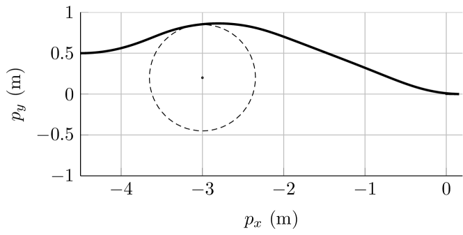
where (px,py)subscript𝑝𝑥subscript𝑝𝑦(p_{x},p_{y}) are the position coordinates of the vehicle with respect to an Earth-fixed frame of reference, ψ𝜓\psi is the vehicle’s orientation and v𝑣v is the longitudinal velocity, which follows a first-order dynamics with parameter α=0.25𝛼0.25\alpha=0.25. The vehicle is controlled by its longitudinal acceleration, a𝑎a, and the steering angle δ𝛿\delta. We define the state vector x=(px,pt,ψ,v)𝑥subscript𝑝𝑥subscript𝑝𝑡𝜓𝑣x=(p_{x},p_{t},\psi,v) and the input vector u=(a,δ)𝑢𝑎𝛿u=(a,\delta). The length of the vehicle is L=0.5m𝐿0.5mL=0.5\,\mathrm{m}. The above dynamical system is discretized with the Euler method with sampling time Ts=50mssubscript𝑇𝑠50msT_{s}=50\,\mathrm{ms}. The vehicle must navigate from an initial position, pose and velocity, x𝑥x, to a target position and pose, xref=(pxref,pyref,ψref,0)superscript𝑥refsuperscriptsubscript𝑝𝑥refsuperscriptsubscript𝑝𝑦refsuperscript𝜓ref0x^{\mathrm{ref}}=(p_{x}^{\mathrm{ref}},p_{y}^{\mathrm{ref}},\psi^{\mathrm{ref}},0), while avoiding a cylindrical obstacle of radius r=0.65𝑟0.65r=0.65 positioned at (3,0.2)30.2(-3,0.2).

We formulate an MPC problem with prediction horizon N=100𝑁100N=100 and stage cost function (x,u)=18(px2+py2)+2ψ2+5v2𝑥𝑢18superscriptsubscript𝑝𝑥2superscriptsubscript𝑝𝑦22superscript𝜓25superscript𝑣2\ell(x,u)=18(p_{x}^{2}+p_{y}^{2})+2\psi^{2}+5v^{2} and the terminal cost function N(x)=1500(px2+py2)+500ψ2+10v2subscript𝑁𝑥1500superscriptsubscript𝑝𝑥2superscriptsubscript𝑝𝑦2500superscript𝜓210superscript𝑣2\ell_{N}(x)=1500(p_{x}^{2}+p_{y}^{2})+500\psi^{2}+10v^{2}. In order to avoid aggressive steering or jerks we introduce the additional stage cost function Δ(ut,ut1)=100(atat1)2+30(δtδt1)2subscriptΔsubscript𝑢𝑡subscript𝑢𝑡1100superscriptsubscript𝑎𝑡subscript𝑎𝑡1230superscriptsubscript𝛿𝑡subscript𝛿𝑡12\ell_{\Delta}(u_{t},u_{t-1}){}={}100(a_{t}-a_{t-1})^{2}+30(\delta_{t}-\delta_{t-1})^{2}. Furthermore, we impose the actuation constraints 1a2m/s21𝑎2msuperscripts2-1\leq a\leq 2\,\nicefrac{\mathrm{m}}{\mathrm{s^{2}}} and |δ|0.25rad14.32𝛿0.25radsuperscript14.32|\delta|\leq 0.25\,\mathrm{rad}\approx 14.32^{\circ}. Then, the state sequence is eliminated as in Equation (5). The obstacle avoidance constraints can be formulated as follows

[r2px2py2]+=0,subscriptdelimited-[]superscript𝑟2superscriptsubscript𝑝𝑥2superscriptsubscript𝑝𝑦20\left[{}r^{2}-p_{x}^{2}-p_{y}^{2}{}\right]_{\scriptscriptstyle+}=0, (25)

which can be accommodated using F2subscript𝐹2F_{2} and the penalty method. Alternatively, in this case we can treat the obstacle constraints as inequality constraints of the form r2px2py20superscript𝑟2superscriptsubscript𝑝𝑥2superscriptsubscript𝑝𝑦20r^{2}-p_{x}^{2}-p_{y}^{2}\leq 0 and describe them using F1subscript𝐹1F_{1}. The two approaches lead to comparable results as shown in Figure 4.
Refer to caption

Figure 2: (Solid line) Path of NMPC-controlled ground vehicle. (Dashed line) Circular obstacle at (xc,yc)=(3,0.2)subscript𝑥𝑐subscript𝑦𝑐30.2(x_{c},y_{c})=(-3,0.2) of radius r=0.65m𝑟0.65mr=0.65\,\mathrm{m}.

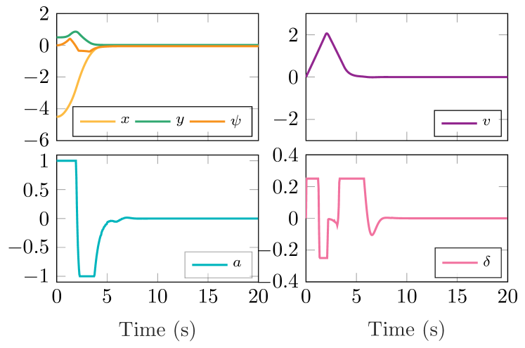
The NMPC-controlled autonomous vehicle manages to avoid the obstacle, arrive at the target position and assume the desired orientation as shown in Figures 2 and 3.
Refer to caption

Figure 3: Closed-loop trajectories for the NMPC-controlled vehicle.

Refer to caption

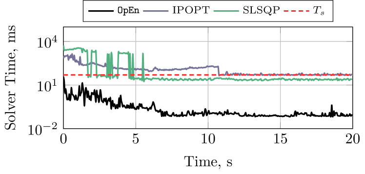
Figure 4: Computation time for the NMPC controlling the autonomous ground vehicle. (Solid lines) Execution times for OpEn, IPOPT and SLSQP, (Dashed line) sampling time.

OpEn outperforms significantly the interior point solver IPOPT and the SQP solver of Python’s package scipy, SLSQP, as illustrated in Figure 4. All software make use of the same auto-generated code to evaluate the cost function, f𝑓f, its gradient, f𝑓\nabla f, and function F2subscript𝐹2F_{2} and the tolerance is set to δ=103𝛿superscript103\delta=10^{-3} and ϵ=104italic-ϵsuperscript104\epsilon=10^{-4}. The selected solver parameters are ϵ0=104subscriptitalic-ϵ0superscript104\epsilon_{0}=10^{-4}, ρ=5𝜌5\rho=5, c0=500subscript𝑐0500c_{0}=500 and L-BFGS memory μ=20𝜇20\mu=20.

5.2 Constrained Nonlinear Estimation

Consider Lorenz’s chaotic system

x˙=[a1(x2x1)x1(a2x3)x2x1x2a3x3]+w(t),˙𝑥matrixsubscript𝑎1subscript𝑥2subscript𝑥1subscript𝑥1subscript𝑎2subscript𝑥3subscript𝑥2subscript𝑥1subscript𝑥2subscript𝑎3subscript𝑥3𝑤𝑡\dot{x}=\begin{bmatrix}a_{1}(x_{2}-x_{1})\\ x_{1}(a_{2}-x_{3})-x_{2}\\ x_{1}x_{2}-a_{3}x_{3}\end{bmatrix}+w(t), (26)

where w𝑤w is a disturbance signal, and parameters a1=10subscript𝑎110a_{1}=10, a2=14subscript𝑎214a_{2}=14, a3=8/3subscript𝑎383a_{3}=\nicefrac{{8}}{{3}}, which we discretize by means of the fourth-order Runge-Kutta method with integration step h=0.10.1h=0.1 leading to a discrete-time system xt+1=Φ(xt)+wtsubscript𝑥𝑡1Φsubscript𝑥𝑡subscript𝑤𝑡x_{t+1}=\Phi(x_{t})+w_{t}. It is known that 1w11𝑤1-1\leq w\leq 1. The system output is given by

y=[2x1x2+x3]G(x)+v,𝑦subscriptmatrix2subscript𝑥1subscript𝑥2subscript𝑥3𝐺𝑥𝑣y=\vphantom{\begin{bmatrix}2x_{1}\\ x_{2}+x_{3}\end{bmatrix}}\smash{\underbracket{\begin{bmatrix}2x_{1}\\ x_{2}+x_{3}\end{bmatrix}}_{G(x)}}+v,\vspace{1.15em} (27)

where v𝑣v is a noise signal for which it is known that 1.5v1.51.5𝑣1.5-1.5\leq v\leq 1.5. We formulate the following constrained nonconvex estimation problem:

(𝒚):minimize𝒙^,𝒘^,𝒗^:𝒚subscriptminimize^𝒙^𝒘^𝒗\displaystyle\mathbb{P}(\mathchoice{\text{\boldmath{$\displaystyle y$}}}{\text{\boldmath{$\textstyle y$}}}{\text{\boldmath{$\scriptstyle y$}}}{\text{\boldmath{$\scriptscriptstyle y$}}}){}:{}\operatorname*{minimize}_{\hat{\mathchoice{\text{\boldmath{$\displaystyle x$}}}{\text{\boldmath{$\textstyle x$}}}{\text{\boldmath{$\scriptstyle x$}}}{\text{\boldmath{$\scriptscriptstyle x$}}}},\hat{\mathchoice{\text{\boldmath{$\displaystyle w$}}}{\text{\boldmath{$\textstyle w$}}}{\text{\boldmath{$\scriptstyle w$}}}{\text{\boldmath{$\scriptscriptstyle w$}}}},\hat{\mathchoice{\text{\boldmath{$\displaystyle v$}}}{\text{\boldmath{$\textstyle v$}}}{\text{\boldmath{$\scriptstyle v$}}}{\text{\boldmath{$\scriptscriptstyle v$}}}}} t=0N1w^tQ2+v^tR2superscriptsubscript𝑡0𝑁1subscriptsuperscriptnormsubscript^𝑤𝑡2𝑄subscriptsuperscriptnormsubscript^𝑣𝑡2𝑅\displaystyle\sum_{t=0}^{N-1}\|\hat{w}_{t}\|^{2}_{Q}+\|\hat{v}_{t}\|^{2}_{R} (28a)
subj.to:\displaystyle\operatorname{subj.\,to:}\, wminw^twmax,tINNformulae-sequencesubscript𝑤minsubscript^𝑤𝑡subscript𝑤max𝑡subscriptIN𝑁\displaystyle w_{\mathrm{min}}\leq\hat{w}_{t}\leq w_{\mathrm{max}},t\in{\rm I\mathchoice{}{}{}{}N}_{N} (28b)
vminv^tvmax,tINNformulae-sequencesubscript𝑣minsubscript^𝑣𝑡subscript𝑣max𝑡subscriptIN𝑁\displaystyle v_{\mathrm{min}}\leq\hat{v}_{t}\leq v_{\mathrm{max}},t\in{\rm I\mathchoice{}{}{}{}N}_{N} (28c)
x^t+1=Φ(x^t)+w^t,tINN1formulae-sequencesubscript^𝑥𝑡1Φsubscript^𝑥𝑡subscript^𝑤𝑡𝑡subscriptIN𝑁1\displaystyle\hat{x}_{t+1}=\Phi(\hat{x}_{t})+\hat{w}_{t},t\in{\rm I\mathchoice{}{}{}{}N}_{N-1} (28d)
yt=G(x^t)+v^t,tINNformulae-sequencesubscript𝑦𝑡𝐺subscript^𝑥𝑡subscript^𝑣𝑡𝑡subscriptIN𝑁\displaystyle y_{t}=G(\hat{x}_{t})+\hat{v}_{t},t\in{\rm I\mathchoice{}{}{}{}N}_{N} (28e)

where Q𝑄Q and R𝑅R are symmetric positive definite matrices. This is a problem with decision variables 𝒙^=(x^t)t=0N^𝒙superscriptsubscriptsubscript^𝑥𝑡𝑡0𝑁\hat{\mathchoice{\text{\boldmath{$\displaystyle x$}}}{\text{\boldmath{$\textstyle x$}}}{\text{\boldmath{$\scriptstyle x$}}}{\text{\boldmath{$\scriptscriptstyle x$}}}}=(\hat{x}_{t})_{t=0}^{N}, 𝒘^=(w^t)t=0N^𝒘superscriptsubscriptsubscript^𝑤𝑡𝑡0𝑁\hat{\mathchoice{\text{\boldmath{$\displaystyle w$}}}{\text{\boldmath{$\textstyle w$}}}{\text{\boldmath{$\scriptstyle w$}}}{\text{\boldmath{$\scriptscriptstyle w$}}}}=(\hat{w}_{t})_{t=0}^{N} and 𝒗^=(v^t)t=0N^𝒗superscriptsubscriptsubscript^𝑣𝑡𝑡0𝑁\hat{\mathchoice{\text{\boldmath{$\displaystyle v$}}}{\text{\boldmath{$\textstyle v$}}}{\text{\boldmath{$\scriptstyle v$}}}{\text{\boldmath{$\scriptscriptstyle v$}}}}=(\hat{v}_{t})_{t=0}^{N}, that is, u=(𝒙^,𝒘^,𝒗^)𝑢^𝒙^𝒘^𝒗u=(\hat{\mathchoice{\text{\boldmath{$\displaystyle x$}}}{\text{\boldmath{$\textstyle x$}}}{\text{\boldmath{$\scriptstyle x$}}}{\text{\boldmath{$\scriptscriptstyle x$}}}},\hat{\mathchoice{\text{\boldmath{$\displaystyle w$}}}{\text{\boldmath{$\textstyle w$}}}{\text{\boldmath{$\scriptstyle w$}}}{\text{\boldmath{$\scriptscriptstyle w$}}}},\hat{\mathchoice{\text{\boldmath{$\displaystyle v$}}}{\text{\boldmath{$\textstyle v$}}}{\text{\boldmath{$\scriptstyle v$}}}{\text{\boldmath{$\scriptscriptstyle v$}}}}), and parameter 𝒚=(yt)t=0N𝒚superscriptsubscriptsubscript𝑦𝑡𝑡0𝑁\mathchoice{\text{\boldmath{$\displaystyle y$}}}{\text{\boldmath{$\textstyle y$}}}{\text{\boldmath{$\scriptstyle y$}}}{\text{\boldmath{$\scriptscriptstyle y$}}}=(y_{t})_{t=0}^{N}.

Constraints (28b) and (28c) define a rectangle, on which one can easily compute projections. The equality constraints (28d) and (28e) are treated with the augmented Lagrangian method by defining

F1(u,𝒚)=[(x^t+1Φ(x^t)w^t)t=0N1(ytG(x^t)v^t)t=0N],subscript𝐹1𝑢𝒚matrixsuperscriptsubscriptsubscript^𝑥𝑡1Φsubscript^𝑥𝑡subscript^𝑤𝑡𝑡0𝑁1superscriptsubscriptsubscript𝑦𝑡𝐺subscript^𝑥𝑡subscript^𝑣𝑡𝑡0𝑁F_{1}(u,\mathchoice{\text{\boldmath{$\displaystyle y$}}}{\text{\boldmath{$\textstyle y$}}}{\text{\boldmath{$\scriptstyle y$}}}{\text{\boldmath{$\scriptscriptstyle y$}}})=\begin{bmatrix}(\hat{x}_{t+1}-\Phi(\hat{x}_{t})-\hat{w}_{t})_{t=0}^{N-1}\\ (y_{t}-G(\hat{x}_{t})-\hat{v}_{t})_{t=0}^{N}\end{bmatrix}, (29)

and C={0}𝐶0C=\{0\}.

Refer to captionRefer to captionRefer to caption

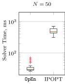
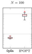
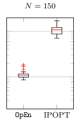
Figure 5: Runtime of OpEn and IPOPT; box plots for 30 random trials.
1010-10001010101010-1000101010101010202020x1subscript𝑥1x_{1}x2subscript𝑥2x_{2}x3subscript𝑥3x_{3}EstimatedActualaaa
Figure 6: Constrained state estimation for Lorenz’s system with N=100𝑁100N=100
1010-1055-500555101010x1subscript𝑥1x_{1}EstimatedActual1010-1000101010x2subscript𝑥2x_{2}0022244466688810101000101010202020303030Time, t𝑡tx3subscript𝑥3x_{3}
Figure 7: States and their estimates for Lorenz’s system using the constrained nonlinear estimation formulation given in (28) with N=100𝑁100N=100

In Figure 5 we compare the runtime of OpEn with IPOPT for N=50𝑁50N=50, N=100𝑁100N=100 and N=150𝑁150N=150. The SQP solver of scipy was significantly slower compared to both OpEn and IPOPT and was therefore omitted. An estimated trajectory for the case N=100𝑁100N=100 is shown in Figure 6. The same data are presented in Figure 7 where the system states and their estimates are plotted against time. The tuning parameters for OpEn were chosen to be c0=200subscript𝑐0200c_{0}=200, ρ=1.8𝜌1.8\rho=1.8, ϵ0=0.1subscriptitalic-ϵ00.1\epsilon_{0}=0.1, μ=15𝜇15\mu=15 and tolerances δ=105𝛿superscript105\delta=10^{-5} and ϵ=104italic-ϵsuperscript104\epsilon=10^{-4}. OpEn performed no more that 7 outer iterations (in the majority of cases, fewer than 5) keeping the penalty parameter, cνsubscript𝑐𝜈c_{\nu}, below 396723967239672.

6 Conclusions and Future work

In this paper we presented a code generation software that can be easily used in Python and MATLAB and will empower engineers to build embedded optimization modules that will underpin complex control, estimation and signal processing developments. The proposed algorithm can handle nonconvex smooth cost functions and nonlinear constraints by means of the augmented Lagrangian and penalty methods, the latter being particularly suitable for obstacle/collision avoidance problems. Future work will focus on the study of the convergence properties of problems that involve constraints of the form (1b) and (1c) under weak assumptions.

References

  • Andersson et al. (2019) J.A.E. Andersson, J. Gillis, G. Horn, J.B. Rawlings, and M. Diehl. CasADi: a software framework for nonlinear optimization and optimal control. Math Prog Comp, 11(1):1–36, 2019.
  • Banjac et al. (2017) G. Banjac, B. Stellato, N. Moehle, P. Goulart, A. Bemporad, and S. Boyd. Embedded code generation using the OSQP solver. In IEEE CDC, 2017.
  • Birgin and Martínez (2014) E.G. Birgin and J.M. Martínez. Practical Augmented Lagrangian Methods for Constrained Optimization (Fundamentals of Algorithms). SIAM, 2014.
  • Ferreau et al. (2017) H.J. Ferreau, S. Almér, R. Verschueren, M. Diehl, D. Frick, A. Domahidi, J.L. Jerez, G. Stathopoulos, and C. Jones. Embedded optimization methods for industrial automatic control. IFAC-PapersOnLine, 50(1):13194 – 13209, 2017.
  • Gill et al. (2005) P.E. Gill, W. Murray, and M.A. Saunders. SNOPT: An SQP algorithm for large-scale constrained optimization. SIAM Review, 47(1):99–131, January 2005.
  • Gopal and Biegler (1998) V. Gopal and L. T. Biegler. Large scale inequality constrained optimization and control. IEEE Control Systems Magazine, 18(6):59–68, Dec 1998.
  • Hermans et al. (2018) B. Hermans, P. Patrinos, and G. Pipeleers. A penalty method based approach for autonomous navigation using nonlinear model predictive control. IFAC-PapersOnLine, 51(20):234 – 240, 2018.
  • Hermans et al. (2019) B. Hermans, G. Pipeleers, and P. Patrinos. A penalty method for nonlinear programs with set exclusion constraints. Submitted to Automatica, 2019.
  • Houska et al. (2011a) B. Houska, H.J. Ferreau, and M. Diehl. ACADO Toolkit – An open source framework for automatic control and dynamic optimization. Optim Contr Appl Meth, 32(3):298–312, 2011a.
  • Houska et al. (2011b) B. Houska, H.J. Ferreau, and M. Diehl. An Auto-Generated Real-Time Iteration Algorithm for Nonlinear MPC in the Microsecond Range. Automatica, 47(10):2279–2285, 2011b.
  • Izmailov et al. (2012) A.F. Izmailov, M.V. Solodov, and E.I. Uskov. Global convergence of augmented lagrangian methods applied to optimization problems with degenerate constraints, including problems with complementarity constraints. SIAM J Optim, 22(4):1579–1606, 2012.
  • Koubaa (2017) A. Koubaa. Robot Operating System (ROS): The Complete Reference, volume 2. Springer, 1st edition, 2017.
  • Kouzoupis et al. (2015) D. Kouzoupis, A. Zanelli, H. Peyrl, and H. J. Ferreau. Towards proper assessment of QP algorithms for embedded model predictive control. In ECC, pages 2609–16, 2015.
  • Kraft (1988) D. Kraft. A software package for sequential quadratic programming. Technical Report DFVLR-FB 88-28, DLR German Aerospace Center – Institute for Flight Mechanics, Köln, Germany, 1988.
  • Li and Fukushima (2001) D.-H. Li and M. Fukushima. On the global convergence of the BFGS method for nonconvex unconstrained optimization problems. SIAM J Optim, 11(4):1054–64, 2001.
  • Matsakis and Klock II (2014) N.D. Matsakis and F.S. Klock II. The Rust language. Ada Lett., 34(3):103–104, Oct 2014.
  • Mattingley and Boyd (2010) J. Mattingley and S. Boyd. Real-time convex optimization in signal processing. IEEE Signal Processing Magazine, 27(3):50–61, May 2010.
  • Mattingley and Boyd (2012) J. Mattingley and S. Boyd. CVXGEN: a code generator for embedded convex optimization. Optimization and Engineering, 13(1):1–27, Mar 2012.
  • Nocedal and Wright (2006) J. Nocedal and S.J. Wright. Numerical Optimization. Springer New York, 2006.
  • Sathya et al. (2018) A. Sathya, P. Sopasakis, R. Van Parys, A. Themelis, G. Pipeleers, and P. Patrinos. Embedded nonlinear model predictive control for obstacle avoidance using PANOC. In ECC, pages 1523–1528, 2018.
  • Scheel and Scholtes (2000) H. Scheel and S. Scholtes. Mathematical programs with complementarity constraints: Stationarity, optimality, and sensitivity. Math. Op. Res., 25(1):1–22, 2000.
  • Shukla et al. (2017) H.A. Shukla, B. Khusainov, E.C. Kerrigan, and C.N Jones. Software and hardware code generation for predictive control using splitting methods. IFAC-PapersOnLine, 50(1):14386 – 14391, 2017.
  • Small et al. (2019) E. Small, P. Sopasakis, E. Fresk, P. Patrinos, and G. Nikolakopoulos. Aerial navigation in obstructed environments with embedded nonlinear model predictive control. In ECC, pages 3556–3563, 2019.
  • Stella et al. (2017) L. Stella, A. Themelis, P. Sopasakis, and P. Patrinos. A simple and efficient algorithm for nonlinear model predictive control. In IEEE CDC, pages 1939–44, 2017.
  • Themelis et al. (2018) A. Themelis, L. Stella, and P. Patrinos. Forward-backward envelope for the sum of two nonconvex functions: Further properties and nonmonotone linesearch algorithms. SIAM J Optim, 28(3):2274–2303, 2018.
  • Varghese et al. (2016) B. Varghese, N. Wang, S. Barbhuiya, P. Kilpatrick, and D. Nikolopoulos. Challenges and opportunities in edge computing. In IEEE SmartCloud, pages 20–26, 2016.
  • Verschueren et al. (2018) R. Verschueren, G. Frison, D. Kouzoupis, N. van Duijkeren, A. Zanelli, R. Quirynen, and M. Diehl. Towards a modular software package for embedded optimization. IFAC-PapersOnLine, 51(20):374 – 380, 2018.
  • Wächter and Biegler (2006) A. Wächter and L.T. Biegler. On the implementation of an interior-point filter line-search algorithm for large-scale nonlinear programming. Math Prog, 106(1):25–57, 2006.
  • Zanelli et al. (2017) A. Zanelli, R. Quirynen, J. Jerez, and M. Diehl. A homotopy-based nonlinear interior-point method for nmpc. IFAC-PapersOnLine, 50(1):13188 – 13193, 2017.
  • Zillober et al. (2004) Ch. Zillober, K. Schittkowski, and K. Moritzen. Very large scale optimization by sequential convex programming. Optim Meth Soft, 19(1):103–120, February 2004.
  • Zometa et al. (2013) P. Zometa, M. Kögel, and R. Findeisen. μ𝜇\muAO-MPC: A free code generation tool for embedded real-time linear model predictive control. In 2013 IEEE ACC, pages 5320–5325, June 2013.