Signatures of the Higgs mode in transport through a normal-metal–superconductor junction

Abstract

A superconductor subject to electromagnetic irradiation in the terahertz range can show amplitude oscillations of its order parameter. However, coupling this so-called Higgs mode to the charge current is notoriously difficult. We propose to achieve such a coupling in a particle-hole-asymmetric configuration using a DC-voltage-biased normal-metal–superconductor tunnel junction. Using the quasiclassical Green’s function formalism, we demonstrate three characteristic signatures of the Higgs mode: (i) The AC charge current exhibits a pronounced resonant behavior and is maximal when the radiation frequency coincides with the order parameter. (ii) The AC charge current amplitude exhibits a characteristic nonmonotonic behavior with increasing voltage bias. (iii) At resonance for large voltage bias, the AC current vanishes inversely proportional to the bias. These signatures provide an electric detection scheme for the Higgs mode.

Introduction.– Manipulating the superconducting (SC) state using tailored light pulses is currently receiving a great deal of attention. Various fascinating phenomena have been reported, including superconductivity enhancement Wyatt et al. (1966); Dayem and Wiegand (1967); Chang and Scalapino (1977); Tikhonov et al. (2018); Curtis et al. (2019); Dehghani et al. (2020), light-induced superconductivity Fausti et al. (2011); Mitrano et al. (2016); Schlawin et al. (2019); Hart et al. (2019), the presence of chiral Majorana modes in chiral superconductors Claassen et al. (2019), and the emergence of the Higgs mode Anderson (1963); Varma (2002); Pekker and Varma (2015); Anderson (2015); Sooryakumar and Klein (1980, 1981); Grasset et al. (2018); Littlewood and Varma (1981, 1982); Matsunaga et al. (2013, 2014); Kemper et al. (2015); Tsuji and Aoki (2015); Collado et al. (2018); Shimano and Tsuji (2020); Katsumi et al. (2018); Silaev et al. (2019); Krull et al. (2016); Moor et al. (2017); Nakamura et al. (2019); Raines et al. (2020); Puviani et al. (2020); Vadimov et al. (2019); Uematsu et al. (2019); Buzzi et al. (2019); Schwarz et al. (2020); Yang and Wu (2020); Puviani et al. (2020).

The Higgs mode is a gapped collective excitation consisting of the oscillation of the order parameter amplitude in a system with spontaneous symmetry breaking Anderson (1963); Varma (2002); Pekker and Varma (2015); Anderson (2015). In a superconductor where the $U(1)$ symmetry is spontaneously broken, the order parameter amplitude can oscillate when the system is coupled to external gauge fields. The presence of a Higgs mode in superconductors with charge density waves was first observed using the Raman-scattering technique Sooryakumar and Klein (1980, 1981); Grasset et al. (2018) and later theoretically interpreted Littlewood and Varma (1981, 1982). However, the excitation and detection of the Higgs mode in superconductors without charge density waves became experimentally possible only in the last decade due to the experimental advance of ultrafast low-energy terahertz (THz) spectroscopy. Clear nonlinear optical signatures indicating the presence of a Higgs mode have been observed using the pump-probe technique in both $s$-wave Matsunaga et al. (2013, 2014); Kemper et al. (2015); Tsuji and Aoki (2015); Shimano and Tsuji (2020) and $d$-wave Katsumi et al. (2018) superconductors. Since the Higgs mode is a scalar excitation, it is expected to couple to the external electromagnetic field in a nonlinear way. A linear coupling enabled by the presence of a supercurrent was theoretically proposed Moor et al. (2017) and experimentally verified Nakamura et al. (2019). Very recently, it was theoretically predicted that a Higgs mode can be observed through its effect in the time-dependent spin current in a ferromagnet-superconductor junction Silaev et al. (2019).

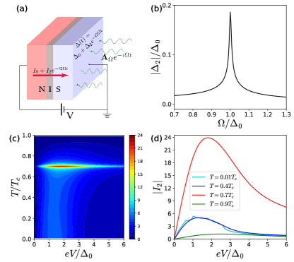
Figure 1: (a) DC-voltage-biased normal-metal–superconductor (NS) junction with a thin insulator (I) acting as a tunnel barrier. The superconductor is subject to electromagnetic irradiation described by a time-dependent vector potential $\mathbf{A}_{\Omega}e^{-i\Omega t}$, which generates a Higgs mode inside the superconductor. (b) $|\Delta_{2}|/\Delta_{0}$ as a function of $\Omega/\Delta_{0}$. The parameters are chosen as $T=0.05T_{c}$, $\gamma=0.01\Delta_{0}|_{T=0}$, and $W_{A}=0.01\Delta_{0}|_{T=0}$. (c) AC charge current $|I_{2}|$ plotted against temperature $T$ and bias voltage $eV$ scaled by the static SC gap amplitude at temperature $T$. The charge currents are in units of $G_{t}W_{A}/e$. The electromagnetic frequency is set to be $\Omega=\Delta_{0}|_{T=0.7T_{c}}$. (d) Line cuts of (c) at different temperatures.

In this work, we consider a junction between a normal metal and an $s$-wave superconductor [see Fig. 1(a)]. THz electromagnetic irradiation can excite a Higgs mode on the SC part of the junction. To couple the Higgs mode to the charge current, particle-hole symmetry has to be broken. Inducing a finite spin splitting in the superconductor is one way to achieve this Silaev et al. (2019). As a potentially simpler alternative, we propose to apply a DC voltage bias to a normal-metal–superconductor (NS) junction. We demonstrate that the Higgs mode will manifest itself in intriguing properties of the AC charge current through the junction [see Fig. 1(c)].

Higgs mode in the superconductor.– We consider a superconductor subject to monochromatic electromagnetic irradiation with the time-dependent vector potential $\mathbf{A}(t)=\mathbf{A}_{\Omega}e^{-i\Omega t}$ in the Coulomb gauge. Due to the nonlinear coupling between the electromagnetic field and the Higgs mode, there will be a second-harmonic correction to the static SC gap $\Delta_{0}$. Thus, the time-dependent order parameter can be expressed as

$$\Delta(t)=\Delta_{0}+\Delta_{2}e^{-i2\Omega t}.$$ (1)

If the irradiation frequency is close to $\Delta_{0}$, superconductivity can possibly be enhanced Chang and Scalapino (1977); Tikhonov et al. (2018), and a small correction to the static order parameter can be incorporated in $\Delta_{0}$.

We employ the quasiclassical Green’s function technique to study the dynamics of the superconductor and the transport properties of the NS junction. The quasiclassical Green’s function $\check{g}_{s}(t,t^{\prime})$ for a dirty superconductor with the diffusion constant $D$ fulfills the time-dependent Usadel equation (Belzig et al., 1999; Kopnin, 2001)

$$i\left\{\check{\tau}_{3}\partial_{t},\check{g}_{s}\right\}+\left[\check{\Delta},\check{g}_{s}\right]-iD\nabla\left(\check{g}_{s}\circ\nabla\check{g}_{s}\right)=0,$$ (2)

where the Green’s function is written in Keldysh space and has the structure

$$\check{g}_{s}=\begin{pmatrix}\hat{g}_{s}^{r}&\hat{g}_{s}^{k}\\ 0&\hat{g}_{s}^{a}\end{pmatrix}.$$ (3)

The order parameter has the form $\check{\Delta}=i\check{\tau}_{2}\Delta$. The matrices $\check{\tau}_{\alpha}$ with $\alpha=1,2,3$ are diagonal matrices with entries $\hat{\tau}_{\alpha}$, that is $\check{\tau}_{\alpha}=\mathrm{diag}[\hat{\tau}_{\alpha},\hat{\tau}_{\alpha}]$, where $\hat{\tau}_{\alpha}$ are the Pauli matrices in Nambu space. In Eq. (2), the anti-commutator is defined as $\left\{\check{\tau}_{3}\partial_{t},\check{g}_{s}\right\}=\check{\tau}_{3}\partial_{t}\check{g}_{s}(t,t^{\prime})+\partial_{t^{\prime}}\check{g}_{s}(t,t^{\prime})\check{\tau}_{3}$, and $\nabla\cdot=\partial_{\mathbf{r}}\cdot-ie[\check{\tau}_{3}\mathbf{A}(t),\cdot]$. The convolution operation between two objects $f$ and $g$ is defined as $(f\circ g)(t,t^{\prime})=\int dt_{1}f(t,t_{1})g(t_{1},t^{\prime})$. The Green’s function obeys the normalization condition $\check{g}_{s}\circ\check{g}_{s}=1$.

Since the Higgs mode couples to the electromagnetic field nonlinearly, to leading order there is a second-harmonic correction $\check{g}_{2}$ to the stationary Green’s function $\check{g}_{0}$,

$$\check{g}_{s}(t,t^{\prime})=\check{g}_{0}(t-t^{\prime})+\check{g}_{2}(t,t^{\prime}).$$ (4)

The Fourier transforms of $\check{g}_{0}$ and $\check{g}_{2}$ are, respectively, defined as

$$\check{g}_{0}(t-t^{\prime}) =\int\frac{d\epsilon}{2\pi}e^{-i\epsilon(t-t^{\prime})}\check{g}_{0}(\epsilon),$$

$$\check{g}_{2}(t,t^{\prime}) =\int\frac{d\epsilon}{2\pi}e^{-i\epsilon_{+}t+i\epsilon_{-}t^{\prime}}\check{g}_{2}(\epsilon_{+},\epsilon_{-}),$$ (5)

with $\epsilon_{\pm}=\epsilon\pm\Omega$. The normalization condition leads to $\check{g}_{2}(\epsilon_{+},\epsilon_{-})\check{g}_{0}(\epsilon_{-})+\check{g}_{0}(\epsilon_{+})\check{g}_{2}(\epsilon_{+},\epsilon_{-})=0$.

For the stationary quasiclassical Green’s functions, we have Kopnin (2001)

$$\hat{g}^{r(a)}_{0}(\epsilon)=g^{r(a)}_{0}(\epsilon)\hat{\tau}_{3}+i\hat{\tau}_{2}f^{r(a)}_{0}(\epsilon),$$ (6)

$$\hat{g}^{k}_{0}(\epsilon)=\left[\hat{g}^{r}_{0}(\epsilon)-\hat{g}^{a}_{0}(\epsilon)\right]\tanh\left(\beta\epsilon/2\right),$$ (7)

where $\beta=1/(k_{B}T)$, and

$$g_{0}^{r(a)}=f_{0}^{r(a)}\epsilon/\Delta_{0}=\epsilon/s_{0}^{r(a)},$$ (8)

with $s_{0}^{r(a)}=i\sqrt{\Delta_{0}^{2}-(\epsilon\pm i\gamma)^{2}}$. Here, $\gamma$ is the phenomenological Dynes broadening parameter. Inserting Eqs. (1) and (4) into the Usadel equation (2) leads to the retarded and advanced components of the nonstationary term Silaev et al. (2019),

$$\hat{g}^{r(a)}_{2}(\epsilon_{+},\epsilon_{-})=\hat{g}^{r(a)}_{V}(\epsilon_{+},\epsilon_{-})+\hat{g}^{r(a)}_{H}(\epsilon_{+},\epsilon_{-}).$$ (9)

The first term $\hat{g}_{V}$ is due to the direct second-order coupling to the vector potential and reads

$$\hat{g}^{r(a)}_{V}(\epsilon_{+},\epsilon_{-})=iW_{A}\left[\frac{\hat{\bar{g}}_{0}(\epsilon)-\hat{g}_{0}(\epsilon_{+})\hat{\bar{g}}_{0}(\epsilon)\hat{g}_{0}(\epsilon_{-})}{s_{+}+s_{-}}\right]^{r(a)},$$ (10)

with $W_{A}=De^{2}|\mathbf{A}_{\Omega}|^{2}$ and $\hat{\bar{g}}_{0}=\hat{\tau}_{3}\hat{g}_{0}\hat{\tau}_{3}$. The second term $\hat{g}_{H}$ describes the effect of the Higgs mode,

$$\hat{g}^{r(a)}_{H}(\epsilon_{+},\epsilon_{-})=i\Delta_{2}\left[\frac{\hat{\tau}_{2}-\hat{g}_{0}(\epsilon_{+})\hat{\tau}_{2}\hat{g}_{0}(\epsilon_{-})}{s_{+}+s_{-}}\right]^{r(a)}.$$ (11)

Both here and in (10), we have used the notation $s_{+}^{r(a)}=i\sqrt{\Delta_{0}^{2}-(\epsilon_{+}\pm i\gamma)^{2}}$ and $s_{-}^{r(a)}=i\sqrt{\Delta_{0}^{2}-(\epsilon_{-}\pm i\gamma)^{2}}$.

An expression for the oscillating part $\Delta_{2}$ of the SC gap can be obtained from the gap equation $\Delta(t)=-i\lambda\mathrm{Tr}[\hat{\tau}_{2}\hat{g}^{k}_{s}(t)]$, where $\lambda$ is the pairing interaction. The details of the derivation can be found in the Supplemental Material SM . The static order parameter $\Delta_{0}$ at temperature $T$ (denoted by $\Delta_{0}|_{T}$) can be well fitted by the interpolation formula

$$\Delta_{0}|_{T}=\Delta_{0}|_{T=0}\tanh(1.74\sqrt{T_{c}/T-1}),$$ (12)

where $T_{c}$ is the critical temperature. To simplify the notation, we will omit the variable $T$ in $\Delta_{0}|_{T}$ at nonzero temperature.

The Dynes broadening parameter and irradiation intensity are fixed as $\gamma=0.01\Delta_{0}|_{T=0}$ and $W_{A}=0.01\Delta_{0}|_{T=0}$ in this work. In Fig. 1(b), we plot the dependence of $\Delta_{2}$ on the irradiation frequency $\Omega$ at temperature $T=0.05T_{c}$. A cusp appears at $\Omega=\Delta_{0}$ (resonant condition) where the oscillation amplitude of the order parameter $|\Delta_{2}|$ is maximal. The resonant behavior is a signature of the Higgs mode and can be identified in nonlinear optical response using the pump-probe technique (Matsunaga et al., 2013, 2014; Kemper et al., 2015; Tsuji and Aoki, 2015; Shimano and Tsuji, 2020).

Normal-metal–superconductor junction.– In the following, we study the transport properties of a DC-voltage-biased NS junction, in which the SC side is subject to electromagnetic irradiation described by a vector potential ${\bf A}(t)=\mathbf{A}_{\Omega}e^{-i\Omega t}$ [see Fig. 1(a)]. The THz electromagnetic field is assumed to exist only on the SC side to avoid possible photon-assisted tunneling processes, and its wave vector is parallel to the transport direction of the junction. The thickness of the superconductor is assumed to be smaller than or comparable to the SC coherence length, so that the order parameter can be treated as homogeneous. For simplicity, we consider a tunnel junction, which is characterized by its conductance $G_{t}$. The retarded, advanced and Keldysh components of the Green’s function for the normal metal are expressed as

$$\hat{g}^{r}_{n}=-\hat{g}^{a}_{n}=\hat{\tau}_{3},$$ (13)

and

$$\hat{g}^{k}_{n}(\epsilon)=2\ \mathrm{diag}\Big{[}\tanh\big{(}\frac{\epsilon-eV}{2k_{B}T}\big{)},\ -\tanh\big{(}\frac{\epsilon+eV}{2k_{B}T}\big{)}\Big{]},$$ (14)

where $V$ is the external voltage bias.

Since the leading perturbation due to the Higgs mode is a second harmonic in $\Omega$, the electric current $I(t)$ can be decomposed in a DC component $I_{0}$ and an AC component $I_{2}$ with $I(t)=I_{0}+I_{2}e^{-i2\Omega t}$. For a tunnel junction, the AC component of the particle current to the first order in the tunnel conductance is

$$I_{2}=\frac{G_{t}}{8e}\int d\epsilon\ \mathrm{Tr}(\hat{\tau}_{3}\hat{X}),$$ (15)

with

$$\hat{X}=\hat{g}^{k}_{n}(\epsilon_{+})\hat{g}^{a}_{2}(\epsilon_{+},\epsilon_{-})-\hat{g}^{r}_{2}(\epsilon_{+},\epsilon_{-})\hat{g}^{k}_{n}(\epsilon_{-}).$$ (16)

Equation (15) implies that $I_{2}|_{eV=0}=0$, since the situation is particle-hole symmetric in the absence of a DC voltage bias. A finite voltage bias can break the symmetry so that the Higgs mode can couple to the charge current. This is in contrast to Ref. (Silaev et al., 2019), where particle-hole asymmetry is due to the exchange field in the superconductor induced by an external magnetic field. A detailed derivation of $I_{2}$ using circuit theory Nazarov (1999); Börlin et al. (2002); Bergeret et al. (2011) can be found in the Supplemental Material SM .

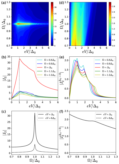
Figure 2: (a) AC charge current $|I_{2}|$ plotted against voltage bias $eV$ and irradiation frequency $\Omega$. Panels (b) and (c) are line cuts of (a) at different $\Omega$ and $eV$, respectively. (d) AC charge current $|I_{2}^{\Delta_{2}=0}|$ in the absence of the Higgs mode, i.e. by artificially setting $\Delta_{2}=0$. Panels (e) and (f) are line cuts of (d) at different $\Omega$ and $eV$, respectively. The charge currents are in units of $G_{t}W_{A}/e$. The temperature is $T=0.05T_{c}$, the other parameters are the same as in Fig. 1(b).

Numerical results.– The gap oscillation amplitude $\Delta_{2}$ is a complex number. This also applies to the AC charge current $I_{2}$, and we focus on discussing the AC charge current magnitude $|I_{2}|$. Figures 2(a), (b) and (c) show the dependence of $|I_{2}|$ on the voltage bias $eV$ and the electromagnetic frequency $\Omega$, where panels (b) and (c) are line cuts of panel (a) for different values of $\Omega$ and $eV$, respectively. To illustrate the influence of the Higgs mode on transport, we artificially set $\Delta_{2}=0$ in $\check{g}_{2}$, that is, $\hat{g}_{2}=\hat{g}_{V}$ from Eq. (9), and calculate the corresponding AC current amplitude $|I_{2}^{\Delta_{2}=0}|$ for comparison [see Figs. 2(d), (e) and (f)]. The charge currents are shown in units of $G_{t}W_{A}/e$.

As can be seen from Fig. 2, the AC charge current amplitude $|I_{2}|$ at a fixed voltage bias shows a pronounced resonant behavior as a function of frequency at $\Omega=\Delta_{0}$, which is not present for $|I_{2}^{\Delta_{2}=0}|$. This can be easily observed by comparing Fig. 2(c) and (f) at $eV=\Delta_{0}$. Also, $|I_{2}|$ is much larger than $|I_{2}^{\Delta_{2}=0}|$ at resonance, since the SC gap oscillation amplitude $|\Delta_{2}|$ achieves its maximum and is much larger than $W_{A}$ as can be seen from Fig. 1(b). Thus, the Higgs mode dominates the AC charge current at resonance. In Fig. S1 in the Supplemental Material SM , we compare the contributions from $\hat{g}_{V}$ and $\hat{g}_{H}$ in the AC charge current amplitude and find that the contribution from $\hat{g}_{V}$ can be even larger than that from $\hat{g}_{H}$ away from resonance. The resonant behavior of $|I_{2}|$ can serve as a signature of the presence of the Higgs mode in the superconductor. A similar observation has been recently reported for spin currents driven by the Higgs mode Silaev et al. (2019).

Figure 2(b) shows that $|I_{2}|$ exhibits an interesting non-monotonic behavior: it increases with increasing voltage bias up to around $eV=\Delta_{0}$, then starts to decrease. At resonance $\Omega=\Delta_{0}$, the AC charge current shows a peak around $eV=\Delta_{0}$. This is explained as follows. The Higgs mode can be interpreted as coherent depairing and pairing of Cooper pairs. The characteristic frequency of the Higgs mode is $2\Delta_{0}$, thus the split quasiparticles (or depaired Cooper pairs) will appear around the SC band edge. Since it is the split quasiparticles that contribute to the AC charge current at resonance, the AC charge current reaches a maximum if the DC voltage bias aligns with the SC band edge at low temperatures. There is also a kink at $eV=3\Delta_{0}$ that can be interpreted as a side band due to the Higgs mode that modulates the quasiparticle density.

Away from resonance, we can observe some other special points in Fig. 2(b). These points are due to the excitation from the electromagnetic irradiation with maxima at $eV=\Delta_{0}$, $-\Delta_{0}+2\Omega$, $\Delta_{0}+\Omega$ and a kink at $\Delta_{0}+2\Omega$ as can be observed from Fig. 2(e). At higher temperatures, the non-monotonic behavior of $|I_{2}|$ still survives, while the maximum point shifts to higher voltages with $eV>\Delta_{0}$ due to thermal excitations (see Fig. S2 in the Supplemental Material SM for $T=0.7T_{c}$).

Under a large bias, the AC charge current $I_{2}$ shows characteristic features: even at $eV=6\Delta_{0}$, a resonant behavior as a function of $\Omega$ can be observed in Fig. 2(c). In contrast, if the Higgs mode is not taken into account, the AC charge current $I_{2}^{\Delta_{2}=0}$ vanishes at large voltage bias even for $\Omega=\Delta_{0}$ as shown in Fig. 2(e). At resonance and with $eV\gg\Delta_{0}$, an analytical estimate given in the Supplemental Material SM shows that the AC current is inversely proportional to the voltage bias, i.e., $I_{2}\propto\Delta_{2}/(eV)$. Thus a finite AC charge current can persist up to relatively large voltage biases. This characteristic behavior of the AC charge current at large bias near resonance can serve as an indicator for the presence of the Higgs mode in the superconductor.

Apart from the possibility to tune the irradiation frequency continuously in experiment Liu et al. (2017, 2020), one can alternatively tune the Higgs mode to be at or away from the resonant condition by changing the system temperature Matsunaga et al. (2014). In Fig. 1(c), we show the AC charge current magnitude as a function of voltage bias and temperature. The electromagnetic frequency is fixed at $\Omega=\Delta_{0}|_{T=0.7T_{c}}\approx 0.8\Delta_{0}|_{T=0}$, which means that the resonance is achieved by tuning the temperature to be at $T=0.7T_{c}$. This leads to a prominent resonant behavior as shown in Fig. 1(c).

Figure 1(d) also shows that $|I_{2}|$ exhibits a nonmonotonic behavior as a function of voltage bias. At a low temperature with $T=0.01T_{c}$, $|I_{2}|$ reaches its maximum around $eV=\Delta_{0}$. It also has maxima at both $0.6\Delta_{0}$ ($\approx-\Delta_{0}+2\Omega$) and $1.8\Delta_{0}$ ($\approx\Delta_{0}+\Omega$) and a kink at $2.6\Delta_{0}$ ($\approx\Delta_{0}+2\Omega$) due to photon-assisted transport processes. Due to thermal excitations, the voltage bias at which $I_{2}$ reaches its maximum increases with increasing temperature. Once the temperature reaches the SC critical temperature, both the static SC gap amplitude and its oscillation vanish, and so does the AC charge current. Similarly to Fig. 2(b), we observe a slow decay $\propto\Delta_{2}/(eV)$ of the AC charge current at large bias near resonance.

Since $\Delta_{2}$ is proportional to $W_{A}$ SM , the next-order correction to the time-dependent order parameter $\Delta(t)$ in Eq. (1) is proportional to $W_{A}^{2}$. Higher-order corrections to $\Delta(t)$ can be ignored if $W_{A}/\Delta_{0}\ll 1$ is satisfied. Given the smallness of $W_{A}/(\Delta_{0}|_{T=0})$, which is $0.01$ in this work, the condition $W_{A}/\Delta_{0}\ll 1$ can be satisfied if the temperature is not too close to $T_{c}$.

The AC current $I_{2}$ is given in units of $G_{t}W_{A}/e$ where $G_{t}$ is the tunnel conductance of the junction and the value chosen for the coupling parameter $W_{A}$ is $W_{A}=0.01\Delta_{0}|_{T=0}$. For example, for the superconductor NbN, $\Delta_{0}|_{T=0}\approx 2.6\,$meV Nakamura et al. (2019), so that the values of $I_{2}$ shown in the figures are approximately in units of $0.026\,{\rm mV}\cdot G_{t}$.

Discussion.– The physical picture that emerges is as follows: the pairing/depairing processes associated with the order-parameter oscillation (Higgs mode) will create particles and holes each of which contribute to the AC tunnel current. At zero voltage bias, their respective contributions cancel. A finite voltage bias leads to particle-hole asymmetry that results in a finite AC current that exhibits signatures of the Higgs mode. On the one hand, this AC charge current may be measured directly. Alternatively, the NS junction can be experimentally manufactured as an antenna, where the electromagnetic irradiation magnitude and frequency due to the AC charge current can be detected. Even though a tunnel junction is studied here, we expect all of the discussed features to be present for a highly transparent junction as well. Note that it is well established that nonequilibrium achieved by voltage biasing can affect the AC response of a superconductor (see, e.g., Catelani et al. (2010)). However, our work considers the inverse situation that the AC response of a superconductor (the Higgs mode) can affect the transport properties of a voltage-biased junction.

The order-parameter oscillation will slowly decay in a power-law way if the electromagnetic irradiation is switched off, and the same applies to the AC charge current. Here, we only treat the steady-state situation with a constant electromagnetic irradiation.

At low temperatures $T\ll\Delta_{0}$, the conductance of the NS-junction that we consider is exponentially suppressed. Thus, for the results presented in Fig. 2, where the temperature is chosen as $T=0.05T_{C}$, we do not expect Joule heating to be a severe problem, and the predicted effects will be unchanged. For the results presented in Fig. 1(c) and (d), if Joule heating exists, the resonant behavior will occur at a lower temperature. However, we expect all the qualitative features to remain.

In the work presented above, the wave vector of the electromagnetic field is assumed to be parallel to the transport direction of the junction. If the wave vector has a finite orthogonal component, the supercurrent, which can be induced by the Andreev reflection processes, will mediate a linear coupling between the Higgs mode and the electromagnetic field Moor et al. (2017); Nakamura et al. (2019); Raines et al. (2020); Puviani et al. (2020). In this case, the time-dependent order parameter can be written as $\Delta(t)=\Delta_{0}+\Delta_{1}e^{-i\Omega t}+\Delta_{2}e^{-i2\Omega t}$ with an additional term of $\Delta_{1}$ compared to Eq. (1). $\Delta_{1}$ and $\Delta_{2}$ exhibit resonances at $\Omega=2\Delta_{0}$ and $\Omega=\Delta_{0}$, respectively. AC charge transport in an NS junction in the presence of a linear coupling between the Higgs mode and the electromagnetic irradiation will be investigated in the future. The generalization to an NS junction with unconventional superconductors Katsumi et al. (2018); Schwarz et al. (2020); Yang and Wu (2020) may also be interesting.

Conclusion.– We have studied the AC transport properties of a DC-voltage-biased NS tunnel junction taking into account the Higgs mode in the superconductor. The pronounced resonant behavior, the characteristic nonmonotonic behavior of the AC charge current with increasing bias and its slow decay inversely proportional to the bias can serve as signatures of the presence of the Higgs mode.

Our results could be applied to design more complex superconducting devices featuring the Higgs dynamics in coupled junctions of superconducting islands. Furthermore, it will be interesting to combine Josephson effects with the Higgs mode.

 

Supplemental Material

I Usadel equation and oscillating part of superconducting order parameter

We consider a monochromatic electromagnetic irradiation with the time-dependent vector potential $\mathbf{A}(t)=\mathbf{A}_{\Omega}e^{-i\Omega t}$. The Higgs mode manifests itself in a time-dependent order parameter,

$$\Delta(t)=\Delta_{0}+\Delta_{2}e^{-i2\Omega t}.$$ (17)

The quasiclassical Green’s function $\check{g}_{s}(t,t^{\prime})$ for a dirty superconductor with the diffusion constant $D$ fulfills the time-dependent Usadel equation Kopnin (2001); Belzig et al. (1999),

$$i\left\{\check{\tau}_{3}\partial_{t},\check{g}_{s}\right\}+\left[\check{\Delta},\check{g}_{s}\right]-iD\nabla\left(\check{g}_{s}\circ\nabla\check{g}_{s}\right)=0.$$ (18)

Here, the anti-commutator is defined as

$$\left\{\check{\tau}_{3}\partial_{t},\check{g}_{s}\right\}=\check{\tau}_{3}\partial_{t}\check{g}_{s}(t,t^{\prime})+\partial_{t^{\prime}}\check{g}_{s}(t,t^{\prime})\check{\tau}_{3},$$ (19)

and $\nabla\cdot=\partial_{\mathbf{r}}\cdot-ie[\check{\tau}_{3}\mathbf{A}(t),\cdot]$. The convolution operation between two objects $f$ and $g$ is defined as

$$(f\circ g)(t,t^{\prime})=\int dt_{1}f(t,t_{1})g(t_{1},t^{\prime}).$$ (20)

The quasiclassical Green’s function is written in Keldysh space and has the structure

$$\check{g}_{s}=\begin{pmatrix}\hat{g}_{s}^{r}&\hat{g}_{s}^{k}\\ &\hat{g}_{s}^{a}\end{pmatrix}.$$ (21)

The superconducting (SC) order parameter has the form $\check{\Delta}=i\check{\tau}_{2}\Delta$. The matrices $\check{\tau}_{\alpha}$ with $\alpha=1,2,3$ are diagonal matrices with entries $\hat{\tau}_{\alpha}$, that is $\check{\tau}_{\alpha}=\mathrm{diag}[\hat{\tau}_{\alpha},\hat{\tau}_{\alpha}]$, where $\hat{\tau}_{\alpha}$ are the Pauli matrices in the Nambu space. The quasiclassical Green’s function obeys the normalization condition $\check{g}_{s}\circ\check{g}_{s}=1$. We will assume all quantities to be uniform within the SC or normal side of the junction. To leading order, the Green’s function and order parameter can be expressed as

$$\check{g}_{s}(t,t^{\prime})=\check{g}_{0}(t-t^{\prime})+\check{g}_{2}(t,t^{\prime}),$$ (22)

where the Fourier transforms of $\check{g}_{0}$ and $\check{g}_{2}$ are defined as

$$\check{g}_{0}(t-t^{\prime}) =\int\frac{d\epsilon}{2\pi}e^{-i\epsilon(t-t^{\prime})}\check{g}_{0}(\epsilon),$$

$$\check{g}_{2}(t,t^{\prime}) =\int\frac{d\epsilon}{2\pi}e^{-i\epsilon_{+}t+i\epsilon_{-}t^{\prime}}\check{g}_{2}(\epsilon_{+},\epsilon_{-}),$$ (23)

with $\epsilon_{\pm}=\epsilon\pm\Omega$. Due to the normalization condition for the stationary Green’s function, $\check{g}_{0}\circ\check{g}_{0}=1$, we obtain $\check{g}_{2}\circ\check{g}_{0}+\check{g}_{0}\circ\check{g}_{2}=0$ which becomes $\check{g}_{2}(\epsilon_{+},\epsilon_{-})\check{g}_{0}(\epsilon_{-})+\check{g}_{0}(\epsilon_{+})\check{g}_{2}(\epsilon_{+},\epsilon_{-})=0$ in the energy domain.

For the stationary quasiclassical Green’s functions, we have Kopnin (2001)

$$\hat{g}^{r(a)}_{0}(\epsilon)=g^{r(a)}_{0}(\epsilon)\hat{\tau}_{3}+i\hat{\tau}_{2}f^{r(a)}_{0}(\epsilon),$$ (24)

$$\hat{g}^{k}_{0}(\epsilon)=\left[\hat{g}^{r}_{0}(\epsilon)-\hat{g}^{a}_{0}(\epsilon)\right]\tanh\left(\beta\epsilon/2\right),$$ (25)

where $\beta=1/(k_{B}T)$, and

$$g_{0}^{r(a)}=f_{0}^{r(a)}\epsilon/\Delta_{0}=\epsilon/s_{0}^{r(a)},$$ (26)

with $s_{0}^{r(a)}=i\sqrt{\Delta_{0}^{2}-(\epsilon\pm i\gamma)^{2}}$. Here, $\gamma$ is the phenomenological Dynes broadening parameter. Inserting Eqs. (17) and (22) into Usadel equation (18) leads to

$$h_{+}\check{g}_{2}(\epsilon_{+},\epsilon_{-})-\check{g}_{2}(\epsilon_{+},\epsilon_{-})h_{-}+\check{\Delta}_{2}\check{g}_{0}(\epsilon_{-})-\check{g}_{0}(\epsilon_{+})\check{\Delta}_{2}$$

$$+iW_{A}\left[\check{\bar{g}}_{0}(\epsilon)\check{g}_{0}(\epsilon_{-})-\check{g}_{0}(\epsilon_{+})\check{\bar{g}}_{0}(\epsilon)\right]=0,$$ (27)

with $h_{\pm}=\epsilon_{\pm}\check{\tau}_{3}+\Delta_{0}i\check{\tau}_{2}$, $W_{A}=De^{2}|\mathbf{A}_{\Omega}|^{2}$, and $\check{\bar{g}}_{0}=\check{\tau}_{3}\check{g}_{0}\check{\tau}_{3}$. By solving Eq. (27), we obtain the retarded and advanced components of the nonstationary term Silaev et al. (2019),

$$\hat{g}^{r(a)}_{2}(\epsilon_{+},\epsilon_{-})=\hat{g}^{r(a)}_{V}(\epsilon_{+},\epsilon_{-})+\hat{g}^{r(a)}_{H}(\epsilon_{+},\epsilon_{-}),$$ (28)

with

$$\hat{g}^{r(a)}_{V}(\epsilon_{+},\epsilon_{-})=iW_{A}\left[\frac{\hat{\bar{g}}_{0}(\epsilon)-\hat{g}_{0}(\epsilon_{+})\hat{\bar{g}}_{0}(\epsilon)\hat{g}_{0}(\epsilon_{-})}{s_{+}+s_{-}}\right]^{r(a)},$$ (29)

and

$$\hat{g}^{r(a)}_{H}(\epsilon_{+},\epsilon_{-})=i\Delta_{2}\left[\frac{\hat{\tau}_{2}-\hat{g}_{0}(\epsilon_{+})\hat{\tau}_{2}\hat{g}_{0}(\epsilon_{-})}{s_{+}+s_{-}}\right]^{r(a)}.$$ (30)

Here,

$$s_{+}^{r(a)}=i\sqrt{\Delta_{0}^{2}-(\epsilon_{+}\pm i\gamma)^{2}},\ \ \ s_{-}^{r(a)}=i\sqrt{\Delta_{0}^{2}-(\epsilon_{-}\pm i\gamma)^{2}},$$

and $\hat{g}^{r(a)}_{V}$ and $\hat{g}^{r(a)}_{H}$ are due to the second order coupling to the vector potential and the Higgs mode, respectively.

The Keldysh component of $\hat{g}^{k}_{2}(\epsilon_{+},\epsilon_{-})$ can be expressed as the sum of a regular part $\hat{g}^{\mathrm{reg}}_{2}$ and an anomalous part $\hat{g}^{\mathrm{an}}_{2}$ Moor et al. (2017); Artemenko and Volkov (1979),

$$\hat{g}^{k}_{2}(\epsilon_{+},\epsilon_{-})=\hat{g}^{\mathrm{reg}}_{2}(\epsilon_{+},\epsilon_{-})+\hat{g}^{\mathrm{an}}_{2}(\epsilon_{+},\epsilon_{-}),$$ (31)

with

$$\hat{g}^{\mathrm{reg}}_{2}=\hat{g}^{r}_{2}(\epsilon_{+},\epsilon_{-})\tanh(\beta\epsilon_{-}/2)-\tanh(\beta\epsilon_{+}/2)\hat{g}^{a}_{2}(\epsilon_{+},\epsilon_{-}),$$ (32)

and

$$\hat{g}^{\mathrm{an}}_{2}(\epsilon_{+},\epsilon_{-})=\hat{g}^{\mathrm{an}}_{V}(\epsilon_{+},\epsilon_{-})+\hat{g}^{\mathrm{an}}_{H}(\epsilon_{+},\epsilon_{-}).$$ (33)

The term $\hat{g}^{\mathrm{an}}_{V}$ is expressed as

$$\hat{g}^{\rm an}_{V}= iW_{A}\frac{[\tanh(\beta\epsilon_{+}/2)-\tanh(\beta\epsilon/2)][\hat{\bar{g}}^{a}_{0}-\hat{g}^{r}_{+}\hat{\bar{g}}^{a}_{0}\hat{g}^{a}_{-}]}{s_{+}^{r}+s_{-}^{a}}$$

$$+ iW_{A}\frac{[\tanh(\beta\epsilon/2)-\tanh(\beta\epsilon_{-}/2)][\hat{\bar{g}}^{r}_{0}-\hat{g}^{r}_{+}\hat{\bar{g}}^{r}_{0}\hat{g}^{a}_{-}]}{s_{+}^{r}+s_{-}^{a}},$$ (34)

with the short notations $\hat{\bar{g}}^{r(a)}_{0}=\hat{\bar{g}}^{r(a)}_{0}(\epsilon)$ and $\hat{g}^{r(a)}_{\pm}=\hat{g}^{r(a)}_{0}(\epsilon_{\pm})$. The term $\hat{g}^{\mathrm{an}}_{H}$ is given by

$$\hat{g}^{\mathrm{an}}_{H}=[\tanh(\beta\epsilon_{+}/2)-\tanh(\beta\epsilon_{-}/2)]\hat{m}^{\mathrm{an}}_{H},$$ (35)

where $\hat{m}^{\mathrm{an}}_{H}$ is obtained by replacing $\hat{g}^{r}_{0}(\epsilon_{-})$ and $s^{r}_{-}$ in the expression of $\hat{g}^{r}_{H}(\epsilon_{+},\epsilon_{-})$ with $\hat{g}^{a}_{0}(\epsilon_{-})$ and $s^{a}_{-}$, respectively.

From the superconducting gap equation Kopnin (2001),

$$\Delta(t)=-i\lambda\mathrm{Tr}[\hat{\tau}_{2}\hat{g}^{k}_{s}(t)],$$ (36)

where $\lambda$ parametrizes the pairing interaction, we have

$$\Delta_{2}\int d\epsilon\ \mathrm{Tr}\left[\hat{\tau}_{2}\hat{g}^{k}_{0}(\epsilon)\right]=\Delta_{0}\int d\epsilon\ \mathrm{Tr}\left[\hat{\tau}_{2}\hat{g}^{k}_{2}(\epsilon_{+},\epsilon_{-})\right].$$ (37)

Lengthy but straightforward calculations lead to

$$\Delta_{2}=iW_{A}\Delta_{0}\frac{B^{r}-B^{a}+B^{\mathrm{an}}}{C^{r}-C^{a}+C^{\mathrm{an}}},$$ (38)

where

$$B^{r(a)} =2\int d\epsilon\ b^{r(a)}(\epsilon)\tanh(\beta\epsilon_{\mp}/2),$$

$$B^{\mathrm{an}} =2\int d\epsilon\ b_{+}^{\mathrm{an}}(\epsilon)\left[\tanh(\beta\epsilon_{+}/2)-\tanh(\beta\epsilon/2)\right]$$

$$+2\int d\epsilon\ b_{-}^{\mathrm{an}}(\epsilon)\left[\tanh(\beta\epsilon/2)-\tanh(\beta\epsilon_{-}/2)\right],$$

$$C^{r(a)} =\int d\epsilon\left[c^{r(a)}(\epsilon)\tanh(\beta\epsilon_{\mp}/2)-\tanh(\beta\epsilon/2)/s^{r(a)}_{0}\right],$$

$$C^{\mathrm{an}} =\int d\epsilon\ c^{\mathrm{an}}(\epsilon)\left[\tanh(\beta\epsilon_{+}/2)-\tanh(\beta\epsilon_{-}/2)\right],$$

with

$$b^{r(a)}(\epsilon) =\left[\frac{\epsilon(\epsilon+\epsilon_{+})s_{-}+\epsilon(\epsilon+\epsilon_{-})s_{+}}{s_{+}s_{0}s_{-}(s_{+}+s_{-})^{2}}\right]^{r(a)},$$

$$b_{+}^{\rm an}(\epsilon) =\frac{\epsilon(\epsilon+\epsilon_{+})s_{-}^{a}+\epsilon(\epsilon+\epsilon_{-})s_{+}^{r}}{s_{+}^{r}s_{0}^{a}s_{-}^{a}(s_{+}^{r}+s_{-}^{a})^{2}},$$

$$b_{-}^{\rm an}(\epsilon) =\frac{\epsilon(\epsilon+\epsilon_{+})s_{-}^{a}+\epsilon(\epsilon+\epsilon_{-})s_{+}^{r}}{s_{+}^{r}s_{0}^{r}s_{-}^{a}(s_{+}^{r}+s_{-}^{a})^{2}},$$

and

$$c^{r(a)}(\epsilon) =\left[\frac{s_{+}s_{-}+\epsilon_{+}\epsilon_{-}+\Delta_{0}^{2}}{s_{+}s_{-}(s_{+}+s_{-})}\right]^{r(a)},$$

$$c^{\rm an}(\epsilon) =\frac{s_{+}^{r}s_{-}^{a}+\epsilon_{+}\epsilon_{-}+\Delta_{0}^{2}}{s_{+}^{r}s_{-}^{a}(s_{+}^{r}+s_{-}^{a})}.$$

One can see that $c^{\mathrm{an}}$ is obtained from $c^{r}$ by replacing $s_{-}^{r}$ with $s_{-}^{a}$.

II AC charge current

The charge current $I(t)$ can be decomposed into a DC component $I_{0}$ and an AC component $I_{2}$ with frequency $2\Omega$,

$$I(t)=I_{0}+I_{2}e^{-i2\Omega t}.$$ (39)

Using circuit theory Nazarov (1999); Börlin et al. (2002); Bergeret et al. (2011), the charge current can be expressed as

$$I(t)=\frac{2\pi}{4e}\mathrm{Tr}\big{[}\hat{\tau}_{3}\hat{I}^{k}(t)\big{]},$$ (40)

with the matrix current

$$\hat{I}^{k}(t)=\frac{G_{t}}{2}\left[\check{g}_{n},\check{g}_{s}\right]^{k}(t,t),$$ (41)

where $G_{t}$ is the tunneling conductance of the NS junction. This leads to the following expressions,

$$I_{0} =\frac{1}{4e}\int d\epsilon\ \mathrm{Tr}\big{[}\hat{\tau}_{3}\hat{I}^{k}_{0}(\epsilon)\big{]},$$ (42)

$$I_{2} =\frac{1}{4e}\int d\epsilon\ \mathrm{Tr}\big{[}\hat{\tau}_{3}\hat{I}^{k}_{2}(\epsilon_{+},\epsilon_{-})\big{]},$$ (43)

with

$$\hat{I}^{k}_{0}(\epsilon)=\frac{G_{t}}{2}\big{[}\hat{g}^{r}_{n}\hat{g}^{k}_{0}(\epsilon)+\hat{g}^{k}_{n}(\epsilon)\hat{g}^{a}_{0}-\hat{g}^{r}_{0}\hat{g}^{k}_{n}(\epsilon)-\hat{g}^{k}_{0}(\epsilon)\hat{g}^{a}_{n}\big{]},$$

$$\hat{I}^{k}_{2}(\epsilon_{+},\epsilon_{-})=\frac{G_{t}}{2}\big{[}\hat{g}^{r}_{n}\hat{g}^{k}_{2}(\epsilon_{+},\epsilon_{-})+\hat{g}^{k}_{n}(\epsilon_{+})\hat{g}^{a}_{2}(\epsilon_{+},\epsilon_{-})$$

$$\qquad\qquad\qquad-\hat{g}^{r}_{2}(\epsilon_{+},\epsilon_{-})\hat{g}^{k}_{n}(\epsilon_{-})-\hat{g}^{k}_{2}(\epsilon_{+},\epsilon_{-})\hat{g}^{a}_{n}\big{]}.$$ (44)

Since $\mathrm{Tr}[\hat{g}^{k}_{2}(\epsilon_{+},\epsilon_{-})]=0$, the AC charge current can be expressed as

$$I_{2}=\frac{G_{t}}{8e}\int d\epsilon\ \mathrm{Tr}(\hat{\tau}_{3}\hat{X}),$$ (45)

with

$$\hat{X}=\hat{g}^{k}_{n}(\epsilon_{+})\hat{g}^{a}_{2}(\epsilon_{+},\epsilon_{-})-\hat{g}^{r}_{2}(\epsilon_{+},\epsilon_{-})\hat{g}^{k}_{n}(\epsilon_{-}).$$ (46)

From this expression, one can verify that the AC charge current vanishes in the absence of the voltage bias, $I_{2}|_{eV=0}=0$. In Fig. 3, we show the contributions from $\hat{g}_{V}^{r(a)}$ and $\hat{g}_{H}^{r(a)}$ in $I_{2}$ using Eqs. (45) and (46). The contributions to $I_{2}$ from $g_{V}$ (denoted as $I_{2}^{\Delta_{2}=0}$) and $g_{H}$ (denoted as $I_{H}$) are calculated by replacing $g_{2}$ in Eq. (46) with $g_{V}$ and $g_{H}$, respectively. At resonance, i.e., $\Omega=\Delta_{0}$, the contribution from $\hat{g}_{V}^{r(a)}$ is much smaller than that from $\hat{g}_{H}^{r(a)}$. This is due to the fact that $|\Delta_{2}|$ achieves its maximum and is much larger than $W_{A}$. For $\Omega=1.1\Delta_{0}$, the contribution from $\hat{g}_{V}^{r(a)}$ cannot be ignored and can be even slightly larger than that from $\hat{g}_{H}^{r(a)}$ at a small voltage bias.

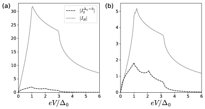
Figure 3: The contributions from $\hat{g}_{V}^{r(a)}$ ($I_{2}^{\Delta_{2}=0}$, dashed lines) and $\hat{g}_{H}^{r(a)}$ ($I_{H}$, dotted lines) in calculating $I_{2}$ using Eqs. (45) and (46) for (a) $\Omega=\Delta_{0}$ and (b) $\Omega=1.1\Delta_{0}$. The currents are given in units of $G_{t}W_{A}/e$.

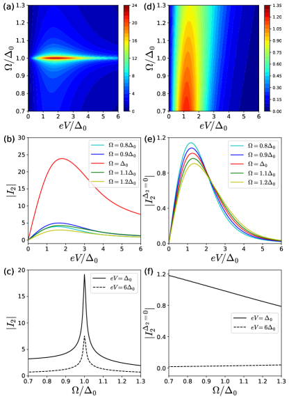
Figure 4: (a) AC charge current $|I_{2}|$ plotted against voltage bias $eV$ and irradiation frequency $\Omega$. Panels (b) and (c) are line cuts of (a) at different $\Omega$ and $eV$, respectively. (d) AC charge current $|I_{2}^{\Delta_{2}=0}|$ in the absence of the Higgs mode, i.e., by artificially setting $\Delta_{2}=0$. Panels (e) and (f) are line cuts of (d) at different $\Omega$ and $eV$, respectively. The parameters are $T=0.7T_{c}$, $\gamma=0.01\Delta_{0}|_{T=0}$, and $W_{A}=0.01\Delta_{0}|_{T=0}$.

We now try to get a compact expression for the AC charge current near resonance with $\Omega\approx\Delta_{0}$ where the contribution from $\hat{g}^{r(a)}_{V}(\epsilon_{+},\epsilon_{-})$ in Eq. (28) can be ignored. Using

$$\hat{g}_{0}^{r}(\epsilon_{+})\hat{\tau}_{2}\hat{g}_{0}^{r}(\epsilon_{-})=2i\Delta_{0}\epsilon/(s_{+}^{r}s_{-}^{r})\hat{\tau}_{3}+u\hat{\tau}_{2},$$ (47)

where the second term $u\hat{\tau}_{2}$ is unimportant in our derivation, Eq. (45) can be expressed as

$$I_{2}=\frac{G_{t}}{2e}\Delta_{2}\Delta_{0}\int d\epsilon\ \epsilon\bigg{[} \frac{\tanh(\frac{\epsilon_{+}-eV}{2k_{B}T})-\tanh(\frac{\epsilon_{+}+eV}{2k_{B}T})}{s_{+}^{a}s_{-}^{a}(s_{+}^{a}+s_{-}^{a})}$$

$$- \frac{\tanh(\frac{\epsilon_{-}-eV}{2k_{B}T})-\tanh(\frac{\epsilon_{-}+eV}{2k_{B}T})}{s_{+}^{r}s_{-}^{r}(s_{+}^{r}+s_{-}^{r})}\bigg{]}.$$ (48)

Using the fact that $[s_{+}^{r(a)}]^{2}-[s_{-}^{r(a)}]^{2}=4(\epsilon\pm i\gamma)\Omega$, this expression can be further simplified as,

$$I_{2}=\frac{G_{t}}{8e}\frac{\Delta_{2}}{\Omega}\int d\epsilon p(\epsilon)\Big{[}\tanh(\frac{\epsilon-eV}{2k_{B}T})-\tanh(\frac{\epsilon+eV}{2k_{B}T})\Big{]},$$ (49)

with

$$p(\epsilon)=\Delta_{0}\bigg{(}\frac{1}{s_{++}^{r}}+\frac{1}{s_{--}^{a}}-\frac{1}{s_{0}^{a}}-\frac{1}{s_{0}^{r}}\bigg{)},$$ (50)

where

$$s_{++}^{r} =i\sqrt{\Delta_{0}^{2}-(\epsilon+2\Omega+i\gamma)^{2}},$$

$$s_{--}^{a} =i\sqrt{\Delta_{0}^{2}-(\epsilon-2\Omega-i\gamma)^{2}}.$$

Since $p(\epsilon)=p(-\epsilon)$, the expression for $I_{2}$ can be reduced to

$$I_{2}=\frac{G_{t}}{4e}\frac{\Delta_{2}}{\Omega}\int d\epsilon p(\epsilon)\tanh(\beta(\epsilon-eV)/2),$$ (51)

which can also be written as

$$I_{2}=\frac{G_{t}}{4e}\frac{\Delta_{2}}{\Omega}\int d\epsilon q(\epsilon)\Big{[}\tanh(\frac{\epsilon_{-}-eV}{2k_{B}T})-\tanh(\frac{\epsilon_{+}-eV}{2k_{B}T})\Big{]},$$ (52)

with

$$q(\epsilon)=\Delta_{0}\left(\frac{1}{s_{+}^{r}}-\frac{1}{s_{-}^{a}}\right).$$ (53)

Since $q(\epsilon)\approx 2\Delta_{0}/\epsilon$ for $\epsilon\gg\Delta_{0}$, we have $I_{2}\propto\Delta_{2}/(eV)$ at large bias with $eV\gg\Delta_{0}$. In other words, at resonance and for large voltage bias, the AC current is inversely proportional to the voltage bias.

Similarly to Fig. (2) in the main text, we show the AC charge current behavior at a large temperature with $T=0.7T_{c}$ in Fig. 4. A resonant behavior can be still observed at $\Omega=\Delta_{0}$. Fig. 4(b) also shows that $|I_{2}|$ exhibits a non-monotonic behavior with increasing bias and vanishes inversely proportional to the bias. Due to thermal excitations, the maximum of $|I_{2}|$ is shifted to larger voltages with $eV>\Delta_{0}$ compared to Fig. (2) in the main text. Kinks and local maxima are smeared by the thermal excitation as well.

References

Wyatt et al. (1966)A. F. G. Wyatt, V. M. Dmitriev, W. S. Moore, and F. W. Sheard, Microwave-enhanced
critical supercurrents in constricted tin films, Phys. Rev. Lett. 16, 1166 (1966).
Dayem and Wiegand (1967)A. H. Dayem and J. J. Wiegand, Behavior of thin-film
superconducting bridges in a microwave field, Phys. Rev. 155, 419 (1967).
Chang and Scalapino (1977)J.-J. Chang and D. J. Scalapino, Gap enhancement in
superconducting thin films due to microwave irradiation, J. Low Temp. Phys. 29, 477 (1977).
Tikhonov et al. (2018)K. S. Tikhonov, M. A. Skvortsov, and T. M. Klapwijk, Superconductivity in the
presence of microwaves: Full phase diagram, Phys. Rev. B 97, 184516 (2018).
Curtis et al. (2019)J. B. Curtis, Z. M. Raines,
A. A. Allocca, M. Hafezi, and V. M. Galitski, Cavity quantum Eliashberg enhancement of
superconductivity, Phys. Rev. Lett. 122, 167002 (2019).
Dehghani et al. (2020)H. Dehghani, Z. M. Raines, V. M. Galitski, and M. Hafezi, Optical enhancement of
superconductivity via targeted destruction of charge density waves, Phys. Rev. B 101, 224506 (2020).
Fausti et al. (2011)D. Fausti, R. I. Tobey,
N. Dean, S. Kaiser, A. Dienst, M. C. Hoffmann, S. Pyon, T. Takayama,
H. Takagi, and A. Cavalleri, Light-induced superconductivity in a stripe-ordered
cuprate, Science 331, 189 (2011).
Mitrano et al. (2016)M. Mitrano, A. Cantaluppi,
D. Nicoletti, S. Kaiser, A. Perucchi, S. Lupi, P. Di Pietro, D. Pontiroli, M. Riccò, S. R. Clark, D. Jaksch, and A. Cavalleri, Possible light-induced
superconductivity in K3C60 at high temperature, Nature 530, 461 (2016).
Schlawin et al. (2019)F. Schlawin, A. Cavalleri, and D. Jaksch, Cavity-mediated
electron-photon superconductivity, Phys. Rev. Lett. 122, 133602 (2019).
Hart et al. (2019)O. Hart, G. Goldstein,
C. Chamon, and C. Castelnovo, Steady-state superconductivity in electronic materials
with repulsive interactions, Phys. Rev. B 100, 060508(R) (2019).
Claassen et al. (2019)M. Claassen, D. M. Kennes, M. Zingl,
M. A. Sentef, and A. Rubio, Universal optical control of chiral
superconductors and Majorana modes, Nat. Phys. 15, 766 (2019).
Sooryakumar and Klein (1980)R. Sooryakumar and M. V. Klein, Raman scattering by
superconducting-gap excitations and their coupling to charge-density waves, Phys. Rev. Lett. 45, 660 (1980).
Sooryakumar and Klein (1981)R. Sooryakumar and M. V. Klein, Raman scattering from
superconducting gap excitations in the presence of a magnetic field, Phys. Rev. B 23, 3213 (1981).
Grasset et al. (2018)R. Grasset, T. Cea,
Y. Gallais, M. Cazayous, A. Sacuto, L. Cario, L. Benfatto, and M.-A. Méasson, Higgs-mode radiance and charge-density-wave order in 2H-NbSe2, Phys. Rev. B 97, 094502 (2018).
Littlewood and Varma (1981)P. B. Littlewood and C. M. Varma, Gauge-invariant theory of
the dynamical interaction of charge density waves and superconductivity, Phys. Rev. Lett. 47, 811 (1981).
Littlewood and Varma (1982)P. B. Littlewood and C. M. Varma, Amplitude collective modes
in superconductors and their coupling to charge-density waves, Phys. Rev. B 26, 4883 (1982).
Matsunaga et al. (2013)R. Matsunaga, Y. I. Hamada, K. Makise,
Y. Uzawa, H. Terai, Z. Wang, and R. Shimano, Higgs amplitude mode in the BCS superconductors
Nb1-xTixN induced by terahertz pulse excitation, Phys. Rev. Lett. 111, 057002 (2013).
Matsunaga et al. (2014)R. Matsunaga, N. Tsuji,
H. Fujita, A. Sugioka, K. Makise, Y. Uzawa, H. Terai, Z. Wang, H. Aoki, and R. Shimano, Light-induced collective
pseudospin precession resonating with Higgs mode in a superconductor, Science 345, 1145 (2014).
Kemper et al. (2015)A. F. Kemper, M. A. Sentef,
B. Moritz, J. K. Freericks, and T. P. Devereaux, Direct observation of Higgs mode oscillations in
the pump-probe photoemission spectra of electron-phonon mediated
superconductors, Phys. Rev. B 92, 224517 (2015).
Tsuji and Aoki (2015)N. Tsuji and H. Aoki, Theory of Anderson pseudospin
resonance with Higgs mode in superconductors, Phys. Rev. B 92, 064508 (2015).
Collado et al. (2018)H. P. O. Collado, J. Lorenzana, G. Usaj, and C. A. Balseiro, Population inversion and dynamical
phase transitions in a driven superconductor, Phys. Rev. B 98, 214519 (2018).
Katsumi et al. (2018)K. Katsumi, N. Tsuji,
Y. I. Hamada, R. Matsunaga, J. Schneeloch, R. D. Zhong, G. D. Gu, H. Aoki, Y. Gallais, and R. Shimano, Higgs mode in the
-wave superconductor Bi2Sr2CaCu2O8+x driven by an
intense terahertz pulse, Phys. Rev. Lett. 120, 117001 (2018).
Silaev et al. (2019)M. A. Silaev, R. Ojajärvi, and T. T. Heikkilä, Spin currents driven by the Higgs mode in
magnetic superconductors (2019), arXiv:1907.00539 .
Krull et al. (2016)H. Krull, N. Bittner,
G. S. Uhrig, D. Manske, and A. P. Schnyder, Coupling of Higgs and Leggett modes in non-equilibrium
superconductors, Nat. Comm. 7, 11921 (2016).
Moor et al. (2017)A. Moor, A. F. Volkov, and K. B. Efetov, Amplitude Higgs mode and admittance
in superconductors with a moving condensate, Phys. Rev. Lett. 118, 047001 (2017).
Nakamura et al. (2019)S. Nakamura, Y. Iida,
Y. Murotani, R. Matsunaga, H. Terai, and R. Shimano, Infrared activation of the Higgs mode by supercurrent injection in
superconducting NbN, Phys. Rev. Lett. 122, 257001 (2019).
Puviani et al. (2020)M. Puviani, L. Schwarz,
X.-X. Zhang, S. Kaiser, and D. Manske, Current-assisted Raman activation of the Higgs mode in
superconductors, Phys. Rev. B 101, 220507 (2020).
Vadimov et al. (2019)V. L. Vadimov, I. M. Khaymovich, and A. S. Mel’nikov, Higgs modes in
proximized superconducting systems, Phys. Rev. B 100, 104515 (2019).
Uematsu et al. (2019)H. Uematsu, T. Mizushima,
A. Tsuruta, S. Fujimoto, and J. A. Sauls, Chiral Higgs mode in nematic superconductors, Phys. Rev. Lett. 123, 237001 (2019).
Buzzi et al. (2019)M. Buzzi, G. Jotzu,
A. Cavalleri, J. I. Cirac, E. A. Demler, B. I. Halperin, M. D. Lukin, T. Shi, Y. Wang, and D. Podolsky, Higgs-mediated optical amplification in a non-equilibrium superconductor
(2019), arXiv:1908.10879 .
Schwarz et al. (2020)L. Schwarz, B. Fauseweh,
N. Tsuji, N. Cheng, N. Bittner, H. Krull, M. Berciu, G. S. Uhrig, A. P. Schnyder, S. Kaiser, and D. Manske, Classification and characterization of
nonequilibrium Higgs modes in unconventional superconductors, Nat. Comm. 11, 287 (2020).
Yang and Wu (2020)F. Yang and M. W. Wu, Theory of Higgs modes in -wave
superconductors (2020), arXiv:2001.06183 .
Belzig et al. (1999)W. Belzig, F. K. Wilhelm,
C. Bruder, G. Schön, and A. D. Zaikin, Quasiclassical Green’s function approach to mesoscopic
superconductivity, Superlattices Microstruct. 25, 1251 (1999).
Kopnin (2001)N. Kopnin, Theory of Nonequilibrium
Superconductivity (Oxford University Press, 2001).
(41)See Supplemental Material for derivations
and additional details.
Börlin et al. (2002)J. Börlin, W. Belzig, and C. Bruder, Full counting statistics of a
superconducting beam splitter, Phys. Rev. Lett. 88, 197001 (2002).
Bergeret et al. (2011)F. S. Bergeret, P. Virtanen,
A. Ozaeta, T. T. Heikkilä, and J. C. Cuevas, Supercurrent and Andreev bound state dynamics in
superconducting quantum point contacts under microwave irradiation, Phys. Rev. B 84, 054504 (2011).
Liu et al. (2017)B. Liu, H. Bromberger,
A. Cartella, T. Gebert, M. Först, and A. Cavalleri, Generation of narrowband, high-intensity, carrier-envelope
phase-stable pulses tunable between 4 and 18 THz, Opt. Lett. 42, 129 (2017).
Liu et al. (2020)B. Liu, M. Först,
M. Fechner, D. Nicoletti, J. Porras, T. Loew, B. Keimer, and A. Cavalleri, Pump frequency
resonances for light-induced incipient superconductivity in
YBa2Cu3O6.5, Phys. Rev. X 10, 011053 (2020).
Catelani et al. (2010)G. Catelani, L. I. Glazman, and K. E. Nagaev, Effect of quasiparticles
injection on the ac response of a superconductor, Phys. Rev. B 82, 134502 (2010).
Artemenko and Volkov (1979)S. N. Artemenko and A. F. Volkov, Electric fields and
collective oscillations in superconductors, Soviet Physics Uspekhi 22, 295 (1979).