High-resolution Monte Carlo study of the order-parameter distribution of the three-dimensional Ising model

Abstract

We apply extensive Monte Carlo simulations to study the probability distribution $P(m)$ of the order parameter $m$ for the simple cubic Ising model with periodic boundary condition at the transition point. Sampling is performed with the Wolff cluster flipping algorithm, and histogram reweighting together with finite-size scaling analyses are then used to extract a precise functional form for the probability distribution of the magnetization, $P(m)$, in the thermodynamic limit. This form should serve as a benchmark for other models in the three-dimensional Ising Universality class.

I introduction

The probability distribution $P(m)$ of the order parameter $m$ is one of the most important quantities for studying the finite-size scaling of critical phenomena. It contains the information needed to calculate all order parameter related quantities such as the susceptibility $\chi=K(\left<m^{2}\right>-\left<m\right>^{2})$, where $K$ is the dimensionless inverse temperature, the Binder cumulant $U=1-\left<m^{4}\right>/(3\left<m^{2}\right>^{2})$, etc. It can also complement the use of critical exponents in determining the critical behavior of a universality class. For these reasons it has been a major research topic in multiple Monte Carlo studies Binder (1981); Bruce and Wilding (1992); Blöte et al. (1995); Kim et al. (1996); Weigel and Janke (2010). With precise calculations of these quantities, one can study the transition temperature and critical behavior of diverse systems, e.g. the 3D Ising Model Ferrenberg and Landau (1991); Ferrenberg et al. (2018), the Lennard-Jones fluid Wilding (1995), and quantum chromodynamics Fukushima and Hatsuda (2011). A very nice application of the magnetization probability distribution function to determine the critical and multicritical universality in several different spin systems can be found in Ref. Plascak and Martins (2013).

According to finite-size scaling theory Binder (1981); Hilfer and Wilding (1995), and assuming hyperscaling and using $L$ (linear dimension), $m$ (order parameter), and $\xi$ (correlation length) as variables, the probability distribution of the order parameter is described by the scaling ansatz,

$$P(m,L,\xi)=L^{\beta/\nu}\tilde{P}(mL^{\beta/\nu},L/\xi)$$ (1)

where $\beta$ is the order parameter exponent, $\nu$ is the correlation length exponent, and $\tilde{P}(mL^{\beta/\nu},L/\xi)$ is the scaling function.

The double peaked distribution of $P(m)$ for the simple cubic Ising model was first numerically calculated by Monte Carlo simulation in Ref. Binder (1981). In Ref. Hilfer and Wilding (1995), systems of size $20^{3}$ and $30^{3}$ were simulated at the critical point and an analytical expression for $P(m)$ was proposed. An improved estimate for $P(m)$ was determined in Ref. Tsypin and Blöte (2000), where the size of the simple cubic lattices ranged from $12^{3}$ to $58^{3}$. That work established a phenomenological formula to describe the peaks of the distribution. In addition to the Ising model, this study tried to extract $P(m)$ in the thermodynamic limit from simulations of the simple cubic, spin-1 Blume-Capel model. The tail of the probability distribution $P(m)$ for the $2D$ Ising model was studied in Ref. Hilfer et al. (2003), but the conclusion was that the true form of the order parameter distribution at criticality was still an open question.

High-resolution numerical estimates for properties of $P(m)$ are important for developing theories and analytical methods for the study of critical phenomena. Our goal in the present paper is to determine the probability distribution of the order parameter at the critical point of the simple cubic Ising model with increased resolution and obtain a more precise expression to describe $P(m)$ in the thermodynamic limit than was heretofore possible.

II model and methods

We consider the $3D$ Ising model on a simple cubic lattice with linear dimension $L$ and periodic boundary conditions. The Hamiltonian is given by,

$$\mathcal{H}=-J\sum_{\langle i,j\rangle}\sigma_{i}\sigma_{j},\;\;\;\;\sigma_{i}=\pm 1$$ (2)

Here $J>0$ is the ferromagnetic coupling, $\langle i,j\rangle$ denotes pairs of nearest-neighbor sites, and the sum is over the $3N$ distinct pairs of nearest-neighbors, where $N=L^{3}$ is the total number of spins. The order parameter (average magnetization) is given by

$$m=\frac{1}{N}\sum_{i}\sigma_{i}$$ (3)

where $i$ denotes each of the $N$ spins, and $-1\leq m\leq 1$.

We performed extensive Monte Carlo simulations using the Wolff cluster flipping algorithm Wolff (1989). The simulations were performed at $K_{0}=0.221\,654$, which was an estimate for the inverse critical temperature used in an earlier, high resolution Monte Carlo study Ferrenberg and Landau (1991). Data were obtained for lattices with $16\leq L\leq 1024$ (for more simulation details, see Ref. Ferrenberg et al. (2018)).

Based on the estimate for the critical point in Ref. Ferrenberg et al. (2018), data were reweighted to $K_{c}=0.221\,654\,626$ using histogram reweighting techniques Ferrenberg and Swendsen (1988, 1989). To obtain the probability distribution $P(m)$ at $K_{c}$, for each occurrence of the order parameter, the corresponding population of the bin of the histogram was incremented by $\exp(-(K_{c}-K_{0})E)$, where $E$ is the total dimensionless energy of the system. The histogram was then normalized to determine $P(m)$.

III results

Fig. 1 shows the scaled probability distribution $P(m)L^{-\beta/\nu}$ as a function of $mL^{\beta/\nu}$ at the critical point $K_{c}=0.221\,654\,626$ for finite lattice sizes ($L=16$, $32$, $96$, and $256$). Here, $\beta$ and $\nu$ are critical exponents for infinite lattices, and $\beta/\nu=0.518\,01(35)$ (Ferrenberg et al., 2018). (We used this estimate in our analysis for consistency since this work uses the same data as that of Ref. Ferrenberg et al. (2018).) The values of the scaled peaks $P(m)L^{-\beta/\nu}$ decreases as the lattice size $L$ increases. Also, systematic deviations from scaling occur in the region of the tails of the distributions. In the thermodynamic limit ($L=\infty$), the probability distribution $P(m)$ is universal up to a rescaling of $m$.

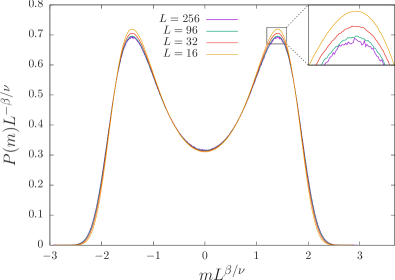
Figure 1: (color online) Scaled probability distribution $P(m)L^{-\beta/\nu}$ as a function of $mL^{\beta/\nu}$ at the critical point $K_{c}=0.221\,654\,626$ Ferrenberg et al. (2018). Curves from the top to the bottom in the inset correspond to lattice sizes $L=16$, $32$, $96$, and $256$ respectively.

First, we took Ref. Tsypin and Blöte (2000) as the blueprint for our analysis. We performed a nonlinear least-squares fit, where the reciprocals of the statistical errors were taken as the weighting factors to the fitting function, with the “improved” ansatz of Ref. Tsypin and Blöte (2000),

$$P(m)=AL^{\beta/\nu}$$

$$\times\exp\left\{-\left[\left(\frac{mL^{\beta/\nu}}{m_{0}}\right)^{2}-1\right]^{2}\left[b\left(\frac{mL^{\beta/\nu}}{m_{0}}\right)^{2}+c\right]\right\}$$ (4)

where $A$, $m_{0}$, $b$, and $c$ are unknown fitting parameters. Note that $m_{0}$ is a scale-invariant (but not universal) quantity.

Fig. 2 shows the difference between the Monte Carlo(MC) data and the fit corresponding to Eq. (III). It also illustrates the error bars for the Monte Carlo data. From Fig. 2 we observe that when the lattice size $L$ is small, e.g. $L=16$, a pattern in the difference between MC data and the fit is very clear. This means that the fitting ansatz, Eq. (III), does not perform well for small $L$ to within the statistical uncertainty. For much larger $L$ (e.g. $L=1024$), the difference between the distribution and the fit to the ansatz is of the same magnitude as the statistical error, so no systematic deviation is observed.

Table 1 shows the results of fitting to Eq. (III). We can tell that the quality of fit is not good when $L\leq 80$, as the value of the $\chi^{2}$ per degree of freedom (d.o.f.) is large. It decreases for larger $L$, and the quality of fit becomes good for the largest lattice sizes.

Table 1: The parameters $m_{0}$, $b$, and $c$ for the probability distribution $P(m)$, fitted to the ansatz Eq. (III). The last column $\chi^{2}$ per degree of freedom (d.o.f.) characterizes the quality of the fit.

$L$	$m_{0}$	$b$	$c$	$\chi^{2}$ per d.o.f.
16	1.411 97 (26)	0.2408 (17)	0.836 86 (77)	381.82
24	1.411 12 (12)	0.209 24 (70)	0.819 38 (40)	70.96
32	1.410 761 (82)	0.195 20 (48)	0.810 45 (21)	24.87
48	1.410 437 (74)	0.181 97 (43)	0.800 87 (25)	6.98
64	1.410 440 (46)	0.176 01 (29)	0.796 07 (26)	3.70
80	1.410 351 (48)	0.172 20 (31)	0.793 03 (33)	2.23
96	1.410 345 (57)	0.169 77 (35)	0.791 04 (34)	1.74
112	1.410 250 (59)	0.167 85 (37)	0.789 39 (42)	1.47
128	1.410 362 (71)	0.166 74 (46)	0.788 09 (36)	1.32
144	1.410 153 (85)	0.165 37 (54)	0.786 93 (37)	1.24
160	1.410 217 (98)	0.164 62 (62)	0.786 39 (42)	1.18
192	1.410 189 (67)	0.163 36 (85)	0.784 99 (46)	1.12
256	1.410 281 (87)	0.1620 (11)	0.783 59 (47)	1.08
384	1.410 18 (11)	0.1560 (14)	0.781 98 (49)	1.04
512	1.410 19 (21)	0.1590 (18)	0.781 01 (63)	1.02
768	1.410 97 (56)	0.1576 (47)	0.781 65 (70)	1.02
1024	1.410 84 (75)	0.1545 (89)	0.780 76 (84)	1.01

Table 2: The parameters $m_{0}$, $a$, $b$, and $c$ for the probability distribution $P(m)$, fitted by the ansatz Eq. (6). The last column $\chi^{2}$ per degree of freedom (d.o.f.) characterizes the quality of the fit.

$L$	$m_{0}$	$a$	$b$	$c$	$\chi^{2}$ per d.o.f.
16	1.408 684 (19)	0.025 01 (21)	0.169 36 (31)	0.839 36 (33)	1.31
24	1.408 497 (27)	0.016 44 (15)	0.160 64 (23)	0.821 24 (36)	1.03
32	1.408 456 (44)	0.013 10 (14)	0.155 53 (12)	0.812 03 (26)	1.04
48	1.408 432 (61)	0.010 46 (15)	0.150 02 (24)	0.802 20 (27)	1.02
64	1.408 588 (49)	0.009 26 (21)	0.147 51 (29)	0.797 27 (31)	1.03
80	1.408 573 (53)	0.008 62 (25)	0.145 55 (40)	0.794 16 (39)	1.02
96	1.408 611 (73)	0.008 22 (27)	0.144 27 (54)	0.792 13 (45)	1.02
112	1.408 564 (70)	0.007 84 (28)	0.143 47 (75)	0.790 43 (51)	1.01
128	1.408 714 (64)	0.007 54 (36)	0.143 26 (61)	0.789 10 (48)	1.02
144	1.408 490 (82)	0.007 48 (45)	0.142 07 (76)	0.787 93 (55)	1.02
160	1.408 580 (92)	0.007 27 (56)	0.141 94 (93)	0.787 36 (48)	1.01
192	1.408 497 (91)	0.007 31 (52)	0.140 53 (99)	0.785 97 (42)	1.01
256	1.408 672 (95)	0.006 75 (65)	0.1409 (12)	0.784 48 (58)	1.01
384	1.408 489 (87)	0.006 57 (74)	0.1396 (20)	0.782 80 (89)	1.01
512	1.408 52 (12)	0.006 35 (93)	0.1395 (25)	0.7817 (13)	1.01
768	1.408 82 (19)	0.0052 (17)	0.1423 (61)	0.7821 (17)	1.01
1024	1.408 73 (27)	0.0043 (27)	0.1440 (90)	0.7806 (25)	1.01

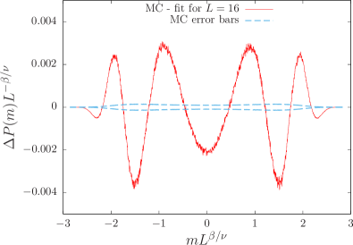
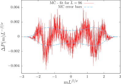
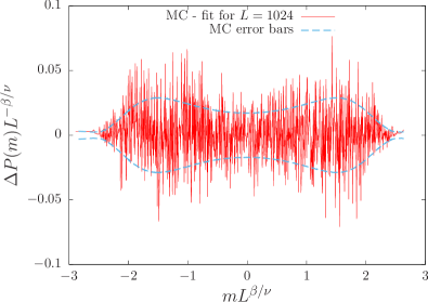
Figure 2: (color online) The red (dark grey) line is the difference between the Monte Carlo data and the fit corresponding to Eq. (III), while the blue (light grey) line is the error bar for the Monte Carlo data (top: $L=16$, middle: $L=96$, bottom: $L=1024$).

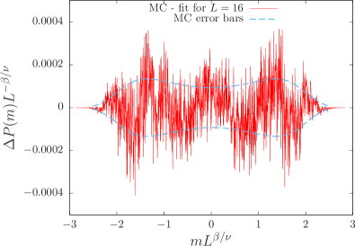
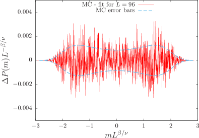
Figure 3: (color online) Analogous to Fig. 2, but the fit is corresponding to Eq. (6) (top: $L=16$, middle: $L=96$, bottom: $L=1024$).

Based on the variance of the fit parameters $b$ and $c$ of Eq. (III) for different lattice sizes, we have estimated their values and errors for $L=\infty$ as follows,

$$b=0.1553(6),\;\;c=0.7783(4)$$ (5)

Ref. Tsypin and Blöte (2000) determined the less precise values $b=0.158(2)$ and $c=0.776(2)$ which agree with our results within the error bars.

The systematic deviation observed for smaller system sizes led us to modify ansatz Eq. (III) by adding various forms of correction terms to see if a revised ansatz could fit the data well even for smaller lattices. We approximated $P(m)$ by using different forms, e.g. adding correction terms in the exponent, adding different correction terms in the pre-exponential factor ($|m|^{\omega},|m|,|m|^{2},...$), and adding correction terms in both the exponent and the pre-exponent factor. We have found that the following “improved” ansatz gives a surprisingly good approximation to $P(m)$ over quite a wide range of $L$ and $m$:

$$P(m)=AL^{\beta/\nu}\exp\left\{-\left[\left(\frac{mL^{\beta/\nu}}{m_{0}}\right)^{2}-1\right]^{2}\left[a\left(\frac{mL^{\beta/\nu}}{m_{0}}\right)^{4}+b\left(\frac{mL^{\beta/\nu}}{m_{0}}\right)^{2}+c\right]\right\}$$ (6)

where $A$, $m_{0}$, $a$, $b$, and $c$ are unknown fit parameters, and as before $\beta/\nu=0.51801(35)$.

Fig. 3 is analogous to Fig. 2, but shows the difference between the Monte Carlo data and the fits to Eq. (6). Fig. 3 shows that even for $L=16$ the residual discrepancy is comparable to the statistical error. If Eq. (6) is used as the fitting function, the maximal difference between MC data and the fit for $L=16$ is around $0.0004$, which is $1/10$ of that in Fig.2 which used Eq. (III) as the fitting function. Thus, the quality of fitting to ansatz Eq. (6) is much higher than that of Eq. (III) for small $L$, and within the statistical errors, Eq. (6) performs better than Eq. (III) as a fitting function.

Results for fitting to the functional form Eq. (6) are shown in Table 2. The values of the $\chi^{2}$ per d.o.f. show that the quality of fit is good even for small lattice sizes. Generally speaking, the error bars for the fit parameters ($m_{0}$, $a$, $b$, and $c$) become larger as $L$ increases. This is because the statistical errors of the raw data are greater for larger lattice sizes (see the dashed line in Fig. 3).

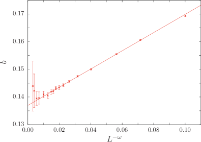
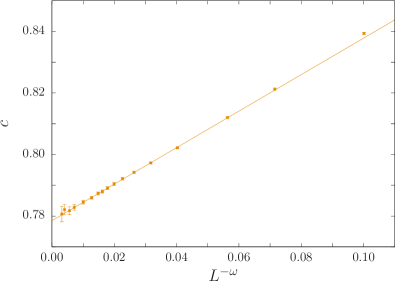
Figure 4: Variation of the fit parameters $a$, $b$, and $c$ for ansatz Eq. (6) as functions of $L^{-\omega}$. The abscissa is chosen so that the leading corrections to scaling are linearized Binder (1981), where $\omega=0.82968(23)$ Simmons-Duffin (2017). The solid lines show extrapolations to $L=\infty$ for $L\geq 32$.

Fig. 4 shows the results of the fit parameters $a$, $b$, and $c$ of the probability distribution $P(m)$, approximated by the ansatz Eq. (6). The horizontal axis is chosen to be $L^{-\omega}$, where $\omega=0.82968(23)$ Simmons-Duffin (2017), so that the leading corrections to scaling are linearized Binder (1981). There is an apparent deviation for $L=768$ and $L=1024$, but the error bars for those sizes are so large that their contributions to the fit are less significant. (There are many more “bins” in the histogram for very large $L$ so there are fewer entries in each bin.) To within statistical errors, there are noticeable finite-size effects for $a$, $b$, and $c$. By doing extrapolations to the thermodynamic limit, their values are estimated as follows,

$$a=0.0052(6),\;\;b=0.137(1),\;\;c=0.7786(3)$$ (7)

Recently, a more precise estimate for $\beta/\nu=0.5181489(10)$ was given by Ref. Simmons-Duffin (2017). If we used this more precise estimate for both ansatzs Eq. (III) and Eq. (6), we will have the same extrapolated values for the parameters.

It is now known that higher order cumulants of the magnetization can have universal values. By using the probability distribution $P(m)$ of the order parameter $m$, we can calculate ratios of moments of the magnetization that are simply related to cumulants:

$$Q_{4} =\langle m^{4}\rangle/\langle m^{2}\rangle^{2},$$

$$Q_{6} =\langle m^{6}\rangle/\langle m^{2}\rangle^{3},$$

$$Q_{8} =\langle m^{8}\rangle/\langle m^{2}\rangle^{4}.$$

Of course, the estimation of the cumulants from the Monte Carlo data depends upon the entire distribution; moreover, as the order of the cumulant increases, the tails of $P(m)$ become increasingly important. Since the tails are effectively truncated by lack of data from the simulation, small biases in cumulant estimates might arise. For high-enough order, truncation will certainly impact the value of the cumulant, For this reason we also generated some large lattice data at a slightly larger coupling and used multi-histogram reweighing to obtain an improved estimate of the contribution of the wings.

Results are shown in Table 3. Eqs. (III, 5) and Eqs. (6, 7) are used together. Error bars are estimated by using the propagation of uncertainty with correlation included (covariances between parameters $a$, $b$, and $c$ are taken into account).

As can be seen in Table 4, we find very small, systematic shifts in the estimates for $Q_{4}$ and $Q_{6}$ that are within the respective error bars of the corrected and uncorrected values. For $Q_{8}$, however, the effect of truncation exceeds the error bars by a substantial amount. Clearly, the estimation of high order moment ratios is not possible without substantially better statistics in the wings

The estimates for $Q_{4}$ and $Q_{6}$ by Eqs. (III, 5) are consistent with those from the extrapolations of our MC data, Ref. Tsypin and Blöte (2000) and Ref. Hasenbusch (2010). Although the estimates by Eqs. (6, 7) are higher than those from our MC data and Ref. Hasenbusch (2010), they still agree with each other to within two error bars. This might be because the estimates of $a$ and $b$ bend off for large system sizes, but the error bars for those sizes are so large that it is not possible to draw a further conclusion.

Table 3: Results for $Q_{4}$ and $Q_{6}$.

	$Q_{4}$	$Q_{6}$
Eqs. (III, 5)	1.603 60 (13)	3.105 55 (62)
Eqs. (6, 7)	1.603 97 (21)	3.107 4 (12)
MC data	1.603 52 (14)	3.105 19 (62)
Typsin and Blöte (2000) Tsypin and Blöte (2000)	1.603 99 (66)	3.106 7 (30)
Hasenbusch (2010) Hasenbusch (2010)	1.603 6 (1)	3.105 3 (5)

Table 4: Corrected and uncorrected estimates for $Q_{4}$, $Q_{6}$ and $Q_{8}$ at $L=512,768$ and 1024.

		$Q_{4}$			$Q_{6}$			$Q_{8}$
$L$	Corrected	Uncorrected	$t$ Statistic	Corrected	Uncorrected	$t$ Statistic	Corrected	Uncorrected	$t$ Statistic
512	1.602 28(10)	1.602 18(10)	-0.707 1	3.099 10(46)	3.098 69(45)	-0.637 1	6.757 2(17)	6.754 4(16)	-1.199 4
768	1.602 22(15)	1.601 98(15)	-1.131 4	3.098 97(68)	3.098 14(68)	-0.863 1	6.758 2(24)	6.753 4(24)	-1.414 2
1024	1.601 97(23)	1.601 49(22)	-1.508 1	3.098 1(11)	3.096 2(10)	-1.278 1	6.769 0(37)	6.746 8(36)	-4.300 4

Comparing the results of fitting to the two ansatzes, Eq. (III) and Eq. (6), one can see that the estimates for $c$ from both fits agree with each other to within error bars. However, the value of $b$ determined for Eq. (III) is larger than that for Eq. (6). We believe that this is a consequence of the correction term corresponding to $b$ in Eq. (III) attempting to account for additional finite-size corrections which are addressed explicitly by the term corresponding to $a$ in Eq. (6).

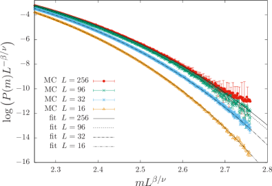
Figure 5: (color online) Logarithm of the tail of the probability distribution of the order parameter (average of the left and right tails), where $mL^{\beta/\nu}\geq 2.25$, for different lattice sizes $L$. The lines are the best fits to Eq. (6). Curves from the top to the bottom correspond to lattice sizes $L=256$, $96$, $32$, and $16$ respectively.

In addition, Fig. 5 shows the logarithm of the tail of the order parameter probability distribution, where $mL^{\beta/\nu}\geq 2.25$. The values of the MC data are the averages of the left and right tails. The solid lines are the best fits to Eq. (6). The tail data for $L=256$ fluctuate too much to present clearly in the figure. Therefore, we applied a smoothing technique, where each data point is the mid-point of a linear fit to 10 sequential points. The shape of the scaled probability distribution differs noticeably from the thermodynamic limit, as there are non-negligible corrections to scaling. The values of $P(m)$ are small in the tail region, and their statistical errors are relatively high, thus, data in the tails contribute less to the fit than those near the peaks. Although their contributions are less significant, Fig. 5 still indicates that the fit by Eq. (6) performs relatively well in the tail region, at least for $mL^{\beta/\nu}\leq 2.75$.

Overall, we have observed that the functional form Eq. (6) permits a high quality, nonlinear least-squares fit to the $P(m)$ data. Although the quality of fit for Eq. (III) is reasonable for large lattice sizes, it is poor for small lattice sizes. The addition of a correction term (Eq. (6)) allows for a high-quality fit for $P(m)$ over a larger range of system sizes. We have observed a noticeable finite-size effect for the fit parameters $a$, $b$, and $c$, thus Eq. (6) is a high-resolution approximation expression for $P(m)$ in the thermodynamic limit.

IV conclusion

We have determined the probability distribution $P(m)$ of the order parameter $m$ for the simple cubic Ising model with periodic boundary conditions at the critical temperature in a high-resolution manner. The high quality of the distribution permitted us to obtain a precise functional form to describe $P(m)$ in the thermodynamic limit as given by Eq. (6). The universal parameters of Eq. (6) have been determined as $a=0.0052(6)$, $b=0.137(1)$, and $c=0.7786(3)$. This expression for $P(m)$ and its parameters provide a valuable benchmark for comparison with results for other models presumed to be in the Ising universality class.