Depth-Adaptive Graph Recurrent Network for Text Classification

Abstract

The Sentence-State LSTM (S-LSTM) Zhang et al. (2018) is a powerful and high efficient graph recurrent network, which views words as nodes and performs layer-wise recurrent steps between them simultaneously. Despite its successes on text representations, the S-LSTM still suffers from two drawbacks. Firstly, given a sentence, certain words are usually more ambiguous than others, and thus more computation steps need to be taken for these difficult words and vice versa. However, the S-LSTM takes fixed computation steps for all words, irrespective of their hardness. The secondary one comes from the lack of sequential information (e.g., word order) that is inherently important for natural language. In this paper, we try to address these issues and propose a depth-adaptive mechanism for the S-LSTM, which allows the model to learn how many computational steps to conduct for different words as required. In addition, we integrate an extra RNN layer to inject sequential information, which also serves as an input feature for the decision of adaptive depths. Results on the classic text classification task (24 datasets in various sizes and domains) show that our model brings significant improvements against the conventional S-LSTM and other high-performance models (e.g., the Transformer), meanwhile achieving a good accuracy-speed trade off.

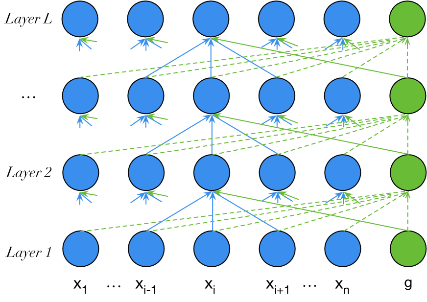
Figure 1: Process of recurrent state transition in the S-LSTM. Given an input sentence with $n$ words, in each layer, the word $x_{i}$ takes information from its predecessor $x_{i-1}$, successor $x_{i+1}$, the global node $g$ and itself to update its hidden state (solid lines). Meanwhile, the global node $g$ takes all local states including itself from the previous layer as context vectors to update global state (dashed line). Both update operations take place simultaneously, and layer-wise parameters are shared.

1 Introduction

Recent advances of graph recurrent network (GRN) have shown impressive performance in many tasks, including sequence modeling Zhang et al. (2018), sentence ordering Yin et al. (2019), machine translation Beck et al. (2018); Guo et al. (2019b), and spoken language understanding Liu et al. (2019). Among these neural networks, the representative S-LSTM has drawn great attention for its high efficiency and strong representation capabilities. More specifically, it views a sentence as a graph of word nodes, and performs layer-wise recurrent steps between words simultaneously, rather than incrementally reading a sequence of words in a sequential manner (e.g., RNN). Besides the local state for each individual word, the S-LSTM preserves a shared global state for the overall sentence. Both local and global states get enriched incrementally by exchanging information between each other. A visual process of recurrent state transition in the S-LSTM is shown in Figure 1.

In spite of its successes, there still exist several limitations in the S-LSTM. For example, given a sentence, certain words are usually more ambiguous than others. Considering this example ‘The film was awesome …’, whether ‘awesome’ means thrilling or excellent is a confusion, thus more contexts should be taken and more layers of abstraction are necessary to refine feature representations. One possible solution is to simply train very deep networks over all word positions, irrespective of their hardness, that is exactly what the conventional S-LSTM does. However, in terms of both computational efficiency and ease of learning, it is preferable to allow model itself to ‘ponder’ and ‘determine’ how many steps of computation to take at each position Graves (2016); Dehghani et al. (2019).

In this paper, we focus on addressing the above issue in the S-LSTM, and propose a depth-adaptive mechanism that enables the model to adapt depths as required. Specifically, at each word position, the executed depth is firstly determined by a specific classifier with corresponding input features, and proceeds to iteratively refine representation until reaching its own executed depth. We also investigate different strategies to obtain the depth distribution, and further endow the model with depth-specific vision through a novel depth embedding.

Additionally, the parallel nature of the S-LSTM makes it inherently lack in modeling sequential information (e.g., word order), which has been shown a highly useful complement to the no-recurrent models Chen et al. (2018); Wang et al. (2019). We investigate different ways to integrate RNN’s inductive bias into our model. Empirically, our experiments indicate this inductive bias is of great matter for text representations. Meanwhile, the informative representations emitted by the RNN are served as input features to calculate the executed depth in our depth-adaptive mechanism.

To evaluate the effectiveness and efficiency of our proposed model, we conduct extensive experiments on the text classification task with 24 datasets in various sizes and domains. Results on all datasets show that our model significantly outperforms the conventional S-LSTM, and other strong baselines (e.g., stacked Bi-LSTM, the Transformer) while achieving a good accuracy-speed trade off. Additionally, our model achieves state-of-the-art performance on 16 out of total 24 datasets.

Our main contributions are as follows:

• We are the first to investigate a depth-adaptive mechanism on graph recurrent network, and significantly boost the performance of the representative S-LSTM model.

• We empirically verify the effectiveness and necessity of recurrent inductive bias for the S-LSTM.

• Our model consistently outperforms strong baseline models and achieves state-of-the-art performance on 16 out of total 24 datasets.

• We conduct thorough analysis to offer more insights and elucidate the properties of our model. Consequently, our depth-adaptive model achieves a good accuracy-speed trade off when compared with full-depth models.

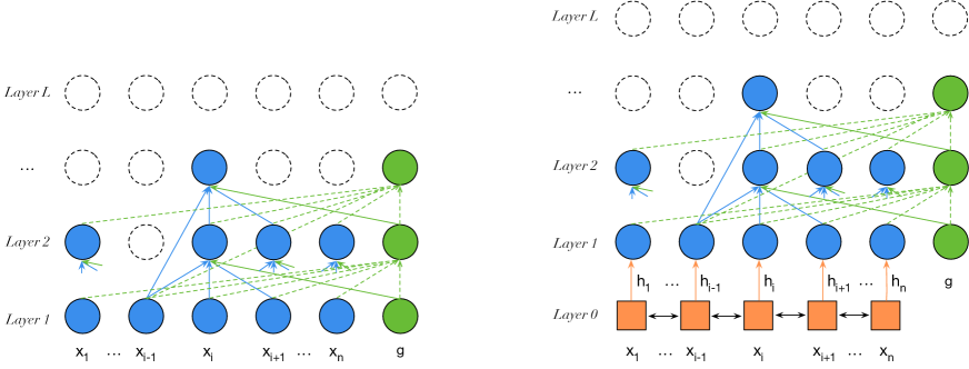
Figure 2: Overview of our proposed model (left part), whose executed depth is varying at different word positions. The dashed nodes indicate that their sates are directly copied from lower layers without computation. In addition, we introduce Bi-RNN (orange squares in the right part) at the bottom layer for two usages: (1) providing sequential information for upper modules, and (2) serving as input features for the calculation of executed depths.

2 Background

Formally, in the $l$-th layer of the S-LSTM, hidden states and cell states can be denoted by:

$$\begin{split}\bm{H}^{l}&=\{\bm{h}_{1}^{l},\bm{h}_{2}^{l},\dots,\bm{h}_{n}^{l},\bm{g}^{l}\}\\ \bm{C}^{l}&=\{\bm{c}_{1}^{l},\bm{c}_{2}^{l},\dots,\bm{c}_{n}^{l},\bm{c}_{g}^{l}\}\end{split}$$ (1)

where $\bm{h}_{i}^{l}$ ($i\in[1,n]$) is the hidden state for the $i$-th word, and $\bm{g}^{l}$ is the hidden state for the entire sentence. Similarly for cell states $\bm{C}^{l}$. Note that $n$ is the number of words for a sentence, and the $0$-th and ($n$+$1$)-th words are padding signals.

As shown in Figure 1, the states transition from $\bm{H}^{l-1}$ to $\bm{H}^{l}$ consists of two parts: (1) word-level transition from $\bm{h}_{i}^{l-1}$ to $\bm{h}_{i}^{l}$; (2) sentence-level transition from $\bm{g}^{l-1}$ to $\bm{g}^{l}$. The former process is computed as follows:

$$\begin{split}\bm{\xi}_{i}^{l}&=\left[\bm{h}_{i-1}^{l-1},\bm{h}_{i}^{l-1},\bm{h}_{i+1}^{l-1}\right]\\ \hat{\bm{l}}_{i}^{l}&=\sigma\left(\bm{W}_{l}\bm{\xi}_{i}^{l}+\bm{U}_{l}\bm{x}_{i}+\bm{V}_{l}\bm{g}^{l-1}+\bm{b}_{l}\right)\\ \hat{\bm{r}}_{i}^{l}&=\sigma\left(\bm{W}_{r}\bm{\xi}_{i}^{l}+\bm{U}_{r}\bm{x}_{i}+\bm{V}_{r}\bm{g}^{l-1}+\bm{b}_{r}\right)\\ \hat{\bm{i}}_{i}^{l}&=\sigma\left(\bm{W}_{i}\bm{\xi}_{i}^{l}+\bm{U}_{i}\bm{x}_{i}+\bm{V}_{i}\bm{g}^{l-1}+\bm{b}_{i}\right)\\ \hat{\bm{f}}_{i}^{l}&=\sigma\left(\bm{W}_{f}\bm{\xi}_{i}^{l}+\bm{U}_{f}\bm{x}_{i}+\bm{V}_{f}\bm{g}^{l-1}+\bm{b}_{f}\right)\\ \hat{\bm{s}}_{i}^{l}&=\sigma\left(\bm{W}_{s}\bm{\xi}_{i}^{l}+\bm{U}_{s}\bm{x}_{i}+\bm{V}_{s}\bm{g}^{l-1}+\bm{b}_{s}\right)\\ \bm{o}_{i}^{l}&=\sigma\left(\bm{W}_{o}\bm{\xi}_{i}^{l}+\bm{U}_{o}\bm{x}_{i}+\bm{V}_{o}\bm{g}^{l-1}+\bm{b}_{o}\right)\\ \bm{u}_{i}^{l}&=\tanh\left(\bm{W}_{u}\bm{\xi}_{i}^{l}+\bm{U}_{u}\bm{x}_{i}+\bm{V}_{u}\bm{g}^{l-1}+\bm{b}_{u}\right)\\ \bm{i}_{i}^{l},&\bm{l}_{i}^{l},\bm{r}_{i}^{l},\bm{f}_{i}^{l},\bm{s}_{i}^{l}=\operatorname{softmax}\left(\hat{\bm{i}}_{i}^{l},\hat{\bm{l}}_{i}^{l},\hat{\bm{r}}_{i}^{l},\hat{\bm{f}}_{i}^{l},\hat{\bm{s}}_{i}^{l}\right)\\ \bm{c}_{i}^{l}&=\bm{l}_{i}^{l}\odot\bm{c}_{i-1}^{l-1}+\bm{f}_{i}^{l}\odot\bm{c}_{i}^{l-1}+\bm{r}_{i}^{l}\odot\bm{c}_{i+1}^{l-1}\\ &\ \ \ \ \ \ \ \ \ \ \ \ \ \ \ \ \ \ \ \ \ +\bm{s}_{i}^{l}\odot\bm{c}_{g}^{l-1}+\bm{i}_{i}^{l}\odot\bm{u}_{i}^{l}\\ \bm{h}_{i}^{l}&=\bm{o}_{l}^{i}\odot\tanh\left(\bm{c}_{i}^{l}\right)\end{split}$$ (2)

where $\bm{\xi}_{i}^{l}$ is the concatenation of hidden states in a window, and $\bm{l}_{i}^{l}$, $\bm{r}_{i}^{l}$, $\bm{f}_{i}^{l}$ and $\bm{s}_{i}^{l}$ are forget gates for left $\bm{c}_{i-1}^{l-1}$, right $\bm{c}_{i+1}^{l-1}$, corresponding $\bm{c}_{i}^{l-1}$ and sentence-level cell state $\bm{c}_{g}^{l-1}$. $\bm{i}_{i}^{l}$ and $\bm{o}_{i}^{l}$ are input and output gates. The value of all gates are normalised such that they sum to $1$. $\bm{W}_{*}$, $\bm{U}_{*}$, $\bm{V}_{*}$ and $\bm{b}_{*}$ ($*\in\{l,r,f,s,i,o,u\}$) are model parameters.

Then the state transition of sentence-level $\bm{g}^{l}$ is computed as follows:

$$\begin{split}\overline{\bm{h}}&=\operatorname{avg}\left(\bm{h}_{1}^{l-1},\bm{h}_{2}^{l-1},\ldots,\bm{h}_{n}^{l-1}\right)\\ \hat{\bm{f}}_{g}^{l}&=\sigma\left(\bm{W}_{g}\bm{g}^{l-1}+\bm{U}_{g}\overline{\bm{h}}+\bm{b}_{g}\right)\\ \hat{\bm{f}}_{i}^{l}&=\sigma\left(\bm{W}_{f}\bm{g}^{l-1}+\bm{U}_{f}\bm{h}_{i}^{l-1}+\bm{b}_{f}\right)\\ \bm{o}^{l}&=\sigma\left(\bm{W}_{o}\bm{g}^{l-1}+\bm{U}_{o}\overline{\bm{h}}+\bm{b}_{o}\right)\\ \bm{f}_{1}^{l}&,\ldots,\bm{f}_{n}^{l},\bm{f}_{g}^{l}=\operatorname{softmax}\left(\hat{\bm{f}}_{1}^{l},\ldots,\hat{\bm{f}}_{n}^{l},\hat{\bm{f}}_{g}^{l}\right)\\ \bm{c}_{g}^{l}&=\bm{f}_{g}^{l}\odot\bm{c}_{g}^{l-1}+\sum_{i}\bm{f}_{i}^{l}\odot\bm{c}_{i}^{l-1}\\ \bm{g}^{l}&=\bm{o}^{l}\odot\tanh\left(\bm{c}_{g}^{l}\right)\end{split}$$ (3)

where $\bm{f}_{1}^{l},\dots,\bm{f}_{n}^{l},\bm{f}_{g}^{l}$ are normalised gates for controlling $\bm{c}_{1}^{l-1},\dots,\bm{c}_{n}^{l-1},\bm{c}_{g}^{l-1}$, respectively. $\bm{o}^{l}$ is an output gate, and $\bm{W}_{*}$, $\bm{U}_{*}$ and $\bm{b}_{*}$ ($*\in\{f,g,o\}$) are model parameters.

3 Model

As the overview shown in Figure 2, our model conducts dynamic steps across different positions, which is more sparse than the conventional S-LSTM drawn in Figure 1. We then proceed to more details of our model in the following sections.

3.1 Token Representation

Given an input sentence $S=\{x_{1},x_{2},\cdots,x_{n}\}$ with $n$ words, we firstly obtain word embeddings $\bm{x}^{glove}$ from the lookup table initialized by Glove. Then we train character-level word embeddings from scratch by Convolutional Neural Network (CNN) Santos and Zadrozny (2014). The glove and character-level embeddings are concatenated to form the final token representations $\bm{X}=\{\bm{x}_{1},\dots,\bm{x}_{n}\}$:

$$\begin{split}\bm{x}_{i}=[\bm{x}_{i}^{glove};\bm{x}_{i}^{char}]\end{split}$$ (4)

3.2 Sequential Module

As mentioned above, the conventional S-LSTM identically treats all positions, and fails to utilize the order of an input sequence. We simply build one layer Bi-LSTMs upon the word embedding layer to inject sequential information (right part in Figure 2), which is computed as follows:

$$\begin{split}&\overrightarrow{\bm{h}_{i}}=\overrightarrow{\bm{LSTM}}(\bm{x}_{i},\overrightarrow{\bm{h}}_{i-1};\bm{\overrightarrow{\theta}})\\ &\overleftarrow{\bm{h}_{i}}=\overleftarrow{\bm{LSTM}}(\bm{x}_{i},\overleftarrow{\bm{h}}_{i+1};\bm{\overleftarrow{\theta}})\\ &\bm{h}_{i}=[\overrightarrow{\bm{h}_{i}};\overleftarrow{\bm{h}_{i}}]\\ \end{split}$$ (5)

where $\bm{\overrightarrow{\theta}}$ and $\bm{\overleftarrow{\theta}}$ are parameter sets of Bi-LSTMs. The output hidden states $\bm{H}=\{\bm{h}_{1},\bm{h}_{2},\dots,\bm{h}_{n}\}$ also serve as input features for the following depth-adaptive mechanism.

3.3 Depth-Adaptive Mechanism

In this section, we describe how to dynamically calculate the depth for each word, and use it to control the state transition process in our model. Specifically, for the $i$-th word ($i\in[1,n]$) in a sentence, its hidden state $\bm{h}_{i}\in\mathbb{R}^{d_{model}}$ is fed to a fully connected feed-forward network Vaswani et al. (2017) to calculate logits value $\bm{l}_{i}$ of depth distribution:

$$\begin{split}\bm{l}_{i}=\max\left(0,\bm{h}_{i}\bm{W}_{1}+\bm{b}_{1}\right)\bm{W}_{2}+\bm{b}_{2}\end{split}$$ (6)

where $\bm{W}_{1}\in\mathbb{R}^{d_{model}\times d_{inner}}$ is a matrix that maps $\bm{h}_{i}$ into an inner vector, and $\bm{W}_{2}\in\mathbb{R}^{d_{inner}\times L}$ is a matrix that maps the inner vector into a $L$-dimensional vector, and $L$ denotes a predefined number of maximum layer. Then the probability ${p}_{i}^{j}$ of the $j$-th depth is computed by $\operatorname{softmax}$:

$$p_{i}^{j}=\frac{e^{l_{i}^{j}}}{\sum_{k=1}^{L}e^{l_{i}^{k}}}\quad\text{ for }j=1,\ldots,L$$ (7)

In particular, we consider three ways to select the depth $d_{i}$ from the probability ${p}_{i}^{j}$.

Hard Selection:

The most direct way is to choose the number with the highest probability from the depth distribution drawn by Eq. (7):

$$d_{i}=\operatorname{argmax}(\bm{p}_{i})$$ (8)

Soft Selection:

A smoother version of selection is to sum up each depth weighted by the corresponding probability. We floor the value considering the discrete nature of the depth distribution by

$$d_{i}=\left\lfloor\sum_{j=0}^{L-1}{j\times p_{i}^{j}}\right\rfloor$$ (9)

Gumbel-Max Selection:

For better simulating the discrete distribution and more robust depth selection, we use Gumbel-Max Gumbel (1954); Maddison et al. (2014), which provides an efficient and robust way to sample from a categorical distribution. Specifically, we add independent Gumbel perturbation $\bm{\eta}_{i}$ to each logit $\bm{l}_{i}$ drawn by Eq. (6):

$$\begin{split}\bm{\eta}_{i}&=-\log(-\log\bm{u}_{i})\\ \widetilde{\bm{l}}_{i}&=(\bm{l}_{i}+\bm{\eta}_{i})/\tau\end{split}$$ (10)

where $\bm{\eta}_{i}$ is computed from a uniform random variable $u\sim\mathcal{U}(0,1)$, and $\tau$ is temperature. As $\tau\rightarrow 0$, samples from the perturbed distribution $\widetilde{\bm{l}}_{i}$ become one-hot, and become uniform as $\tau\rightarrow\infty$. After that, the exact number of depth $d_{i}$ is calculated by modifying the Eq. (7) to:

$$p_{i}^{j}=\frac{e^{\widetilde{l}_{i}^{j}}}{\sum_{k=1}^{L}e^{\widetilde{l}_{i}^{k}}}\quad\text{ for }j=1,\ldots,L$$ (11)

Empirically, we set a tiny value to $\tau$, so the depth distribution calculated by Eq. (11) is in the form of one-hot. Note that Gumbel perturbations are merely used to select depths, and they would not affect the loss function for training.

Dataset	Classes	Type	Average   Lenghts	Max   Lengths	Train    Sample	Test   Sample
TREC Li and Roth (2002)	6	Question	12	39	5,952	500
AG’s News Zhang et al. (2015)	4	Topic	44	221	120,000	7,600
DBPedia Zhang et al. (2015)	14	Topic	67	3,841	560,000	70,000
Subj Pang and Lee (2004)	2	Sentiment	26	122	10,000	CV
MR Pang and Lee (2005)	2	Sentiment	23	61	10,622	CV
Amazon-16 Liu et al. (2017) *	2	Sentiment	133	5,942	31,880	6,400
IMDB Maas et al. (2011)	2	Sentiment	230	2,472	25,000	25,000
Yelp Polarity Zhang et al. (2015)	2	Sentiment	177	2,066	560,000	38,000
Yelp Full Zhang et al. (2015)	5	Sentiment	179	2,342	650,000	50,000

Table 1: Dataset statistics. ‘CV’ means that there was no standard train/test split and thus 10-fold CV was used. ‘$*$’: There are 16 subsets with the same size in Amazon-16, named as Apparel, Baby, Books, Camera, DVD, Electronics, Health, IMDB, Kitchen, Magazines, MR, Music, Software, Sports, Toys and Video.

After acquiring the depth number $d_{i}$ for each individual word, additional efforts should be taken to connect the depth number $d_{i}$ with corresponding steps of computation. Since our model has no access to explicit supervision for depth, in order to make our model learn such relevance, we must inject some depth-specific information into our model. To this end, we preserve a trainable depth embedding $\bm{x}^{depth}$ whose parameters are shared with the $\bm{W}_{2}$ in the above feed-forward network in Eq. (6). We also sum a sinusoidal depth embedding with $\bm{x}^{depth}$ for the similar motivation with the Transformer Vaswani et al. (2017):

$$\begin{split}DE_{(d,2j)}&=\sin(d/10000^{2j/dim_{emb}})\\ DE_{(d,2j+1)}&=\cos(d/10000^{2j/dim_{emb}})\\ \end{split}$$ (12)

where $d$ is the depth, $dim_{emb}$ is the the dimension of the depth embedding, and $j$ is index of $dim_{emb}$. As thus, the final token representation described by Eq. (4) is refined by:

$$\begin{split}\bm{x}_{i}=[\bm{x}_{i}^{glove};\bm{x}_{i}^{char};\bm{x}_{i}^{depth}]\end{split}$$ (13)

Then our model proceeds to perform dynamic state transition between words simultaneously. More specifically, once a word $x_{i}$ reaches its own maximum layer $d_{i}$, it will stop state transition, and simply copy its state to the next layer until all words stop or the predefined maximum layer $L$ is reached. Formally, for the $i$-th word, its hidden state $\bm{h}_{i}$ is updated as follows:

$$\bm{h}_{i}^{l}=\begin{cases}\bm{h}_{i}^{l-1}\text{ \ \ \ \ \ \ \ \ \ \ \ \ \ \ \ \ \ \ \ \ \ \ \ \ \ \ \ \ \ \ \ \ \ \ \ \ \ \ \ \ \ \ \ \ \ \ if $l>d_{i}$}\\ S\textrm{-}LSTM(\bm{x}_{i},\bm{h}_{i-1}^{l-1},\bm{h}_{i}^{l-1},\bm{h}_{i+1}^{l-1},\bm{g}^{l-1})\text{\ else}\end{cases}$$ (14)

where $l\in[1,d_{max}]$ refers to the number of current layer, and $d_{max}$ is the maximum depth in current sentence. Specially, $\bm{h}_{i}^{0}$ is initialized by a linear transformation of the inner vector in Eq. (6). $S\textrm{-}LSTM(\cdot)$ is the state transition function drawn by Eq. (2). As the global state $\bm{g}$ is expected to encode the entire sentence, it conducts $d_{max}$ steps by default, which is drawn by Eq. (3).

3.4 Task-specific Settings

After dynamic steps of computation among all nodes, we build task-specific models for the classification task. The output hidden states of the final layer $\bm{H}^{d_{max}}$ are firstly reduced by max and mean pooling. We then take the concatenations of these two reduced vectors and global states $\bm{g}^{d_{max}}$ to form the final feature vector $\bm{v}$. After the ReLU activation, $\bm{v}$ is fed to a softmax classification layer. Formally, the above-mentioned procedures are computed as follows:

$$\begin{split}&\bm{v}=\operatorname{ReLU}([\mathop{\max}(\bm{H}^{d_{max}});\operatorname{mean}({\bm{H}}^{d_{max}});\bm{g}^{d_{max}}])\\ &P(\widetilde{y}|\bm{v})=\operatorname{softmax}(\bm{W}_{cls}\bm{v}+\bm{b}_{cls})\end{split}$$ (15)

where $P(\widetilde{y}|\bm{v})$ is the probability distribution over the label set, and $\bm{W}_{cls}$ and $\bm{b}_{cls}$ are trainable parameters. Afterwards, the most probable label $\hat{y}$ is chosen from the above probability distribution drawn by Eq. (15), computed as:

$$\begin{split}&\hat{y}=\mathop{\arg\max}P(\widetilde{y}|\bm{v})\\ \end{split}$$ (16)

For training, we denote $y_{i}$ as golden label for the $i$-th sample, and $|S|$ as the size of the label set, then the loss function is computed as cross entropy:

$$\begin{split}&loss=-\sum\limits_{i=1}^{|S|}{y_{i}}log(P_{i}(\widetilde{y}|\bm{v}))\\ \end{split}$$ (17)

4 Experiments

Data / Model	MS-Trans.	Transformer $\dagger$	Star-Trans. $\dagger$	3L-BiLSTMs $\dagger$	S-LSTM $\dagger$	RCRN	Ours
Apparel	86.5	87.3	88.7	89.2	89.8	90.5	91.0
Baby	86.3	85.6	88.0	88.5	89.3	89.0	89.8
Books	87.8	85.3	86.9	87.2	88.8	88.0	89.0
Camera	89.5	89.0	91.8	89.7	91.5	90.5	92.3
Dvd	86.5	86.3	87.4	86.0	89.0	86.8	88.8
Electronics	84.3	86.5	87.2	87.0	86.8	89.0	88.3
Health	86.8	87.5	89.1	89.0	89.0	90.5	90.8
Imdb	85.0	84.3	85.0	88.0	87.6	89.8	89.5
Kitchen	85.8	85.5	86.0	84.5	86.6	86.0	88.5
Magazines	91.8	91.5	91.8	92.5	93.3	94.8	94.3
Mr	78.3	79.3	79.0	77.7	79.0	79.0	79.8
Music	81.5	82.0	84.7	85.7	84.0	86.0	86.5
Software	87.3	88.5	90.9	90.3	90.3	90.8	91.5
Sports	85.5	85.8	86.8	86.5	86.0	88.0	87.0
Toys	87.8	87.5	85.5	90.5	88.0	90.8	91.0
Video	88.4	90.0	89.3	87.8	89.6	88.5	90.2
Avg	86.2	86.4	87.4	87.5	88.0	88.6	89.3

Table 2: Accuracy scores (%) on the Amazon-16 datasets. $\dagger$ is our implementations with several recent advanced techniques (e.g., label smoothing) under the unified setting. We establish new state-of-the-art results on 12 of total 16 datasets, and outperform the existing highest average score (+0.7%).

Models / Dataset	TREC	MR	Subj	IMDB	AG.	DBP.	Yelp P.	Yelp F.	Avg.
RCRN Tay et al. (2018)	96.20	–	–	92.80	–	–	–	–	–
Cove McCann et al. (2017)	95.80	–	–	91.80	–	–	–	–	–
Text-CNN Kim (2014)	93.60	81.50	93.40	–	–	–	–	–	–
Multi-QT Logeswaran and Lee (2018)	92.80	82.40	94.80	–	–	–	–	–	–
AdaSent Zhao et al. (2015)	92.40	83.10	95.50	–	–	–	–	–	–
CNN-MCFA Amplayo et al. (2018)	94.20	81.80	94.40	–	–	–	–	–	–
Capsule-B Yang et al. (2018)	92.80	82.30	93.80	–	92.60	–	–	–	–
DNC+CUW Le et al. (2019)	–	–	–	–	93.90	–	96.40	65.60	–
Region-Emb Qiao et al. (2018)	–	–	–	–	92.80	98.90	96.40	64.90	–
Char-CNN Zhang et al. (2015)	–	–	–	–	90.49	98.45	95.12	62.05	–
DPCNN Johnson and Zhang (2017)	–	–	–	–	93.13	99.12	97.36	69.42	–
DRNN Wang (2018)	–	–	–	–	94.47	99.19	97.27	69.15	–
SWEM-concat Shen et al. (2018)	92.20	78.20	93.00	–	92.66	98.57	95.81	63.79	–
Star-Transformer Guo et al. (2019a) $\dagger$	93.00	79.76	93.40	94.52	92.50	98.62	94.20	63.21	88.65
Transformer Vaswani et al. (2017) $\dagger$	92.00	80.75	94.00	94.58	93.66	98.27	95.07	63.40	88.97
S-LSTM Zhang et al. (2018) $\dagger$	96.00	82.92	95.10	94.92	94.55	99.02	96.22	65.37	90.51
3L-BiLSTMs Hochreiter and Schmidhuber (1997) $\dagger$	95.60	83.50	95.30	93.89	93.99	98.97	96.86	66.86	90.62
Ours	96.40	83.42	95.50	96.27	94.93	99.16	97.34	70.14	91.64

Table 3: Accuracy scores (%) on modestly sized and large-scaled datasets. $\dagger$ is our implementations with several recent advanced techniques and analogous parameter sizes. Our model achieves new state-of-the art results on 4 of 8 datasets under the same settings.

4.1 Task and Datasets

Text classification is a classic task for NLP, which aims to assign a predefined category to free-text documents Zhang et al. (2015), and is generally evaluated by accuracy scores. Generally, The number of categories may range from two to more, which correspond to binary and fine-grained classification. We conduct extensive experiments on the 24 popular datasets collected from diverse domains (e.g., sentiment, question), and range from modestly sized to large-scaled. The statistics of these datasets are listed in Table 1.

4.2 Implementation Details

We apply dropout Srivastava et al. (2014) to word embeddings and hidden states with a rate of 0.3 and 0.2 respectively. Models are optimized by the Adam optimizer Kingma and Ba (2014) with gradient clipping of 5 Pascanu et al. (2013). The initial learning rate $\alpha$ is set to 0.001, and decays with the increment of training steps. For datasets without standard train/test split, we adopt 5-fold cross validation. For datasets without a development set, we randomly sample 10% training samples as the development set . One layer CNN with a filter of size 3 and max pooling are utilized to generate 50d character-level word embeddings. The novel depth embedding is a trainable matrix in 50d. The cased 300d Glove is adapted to initialize word embeddings, and keeps fixed when training. We conduct hyper-parameters tuning to find the proper value of layer size $L$ (finally set to 9), and empirically set hidden size to 400 , temperature $\tau$ to 0.001.

4.3 Main Results

Please note that current hot pre-trained language models (e.g., BERT Devlin et al. (2019), XLNet Yang et al. (2019)) are not directly comparable with our work due to their huge additional corpora. We believe further improvements when utilizing these orthogonal works.

Results on Amazon-16.

The results on 16 Amazon reviews are shown in Table 2, where our model achieves state-of-the-art results on 12 datasets, and reports a new highest average score. The average score gains over 3-layer stacked Bi-LSTMs (+1.8%), and the S-LSTM (+1.3%) are also notable. Strong baselines such as Star-Transformer Guo et al. (2019a) and Recurrently Controlled Recurrent Networks (RCRN) Tay et al. (2018) are also outperformed by our model.

#	Model	Accuracy	$\Delta_{acc}$	Speed	$\Delta_{speed}$
0	Ours	96.27 $\pm$ 0.13	–	57 $\pm$ 1.7	–
1	w/o adaptive-depth mechanism	96.10 $\pm$ 0.08	-0.17	16 $\pm$ 0.3	-41
2	w/o Bi-LSTMs	95.25 $\pm$ 0.25	-1.02	49 $\pm$ 1.3	-8
3	w/ sinusoidal position embedding	95.61 $\pm$ 0.19	-0.66	63 $\pm$ 1.1	+6
4	w/ learned position embedding	95.72 $\pm$ 0.15	-0.55	60 $\pm$ 1.0	+3
–	w/o Gumbel Max	–	–	–	–
5	w/ hard selection	95.65 $\pm$ 0.39	-0.62	57 $\pm$ 1.2	0
6	w/ soft selection	95.71 $\pm$ 0.57	-0.56	57 $\pm$ 1.4	0

Table 4: Ablation experiments on IMDB test set. We run each model variant for three times and report the mean and standard deviation. ‘$\Delta_{acc}$’ and ‘$\Delta_{speed}$’ denote relative improvements of accuray and speed over ‘Ours’ respectively. e.g., the ‘+6’ in ‘$\Delta_{speed}$’ denotes the variant processes 6 more samples than ‘Ours’ per second.

Results on larger benchmarks.

From the results on larger corpora listed in Table 3, we also observe consistent and significant improvements over the conventional S-LSMT (+1.1%) and other strong baseline models (e.g., the transformer (+2.9%), the star-transformer (+3.0%)). More notably, the superiority of our model over baselines are more obvious with the growth of corpora size. Given only training data and the ubiquitous word embeddings (Glove), our model achieves state-of-the-art performance on the TREC, IMDB, AGs News and Yelp Full datasets, and comparable results on other sets.

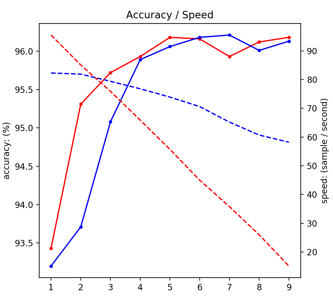
Figure 3: Accuracy and speed   for full-depth (red lines) and adaptive-depth (blue lines) models on the IMDB test set, where X-axis refer to the maximum of layer $L$, and accuracy/speed are drawn by solid/dashed lines, respectively.

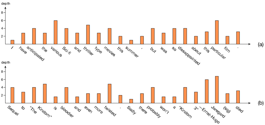
Figure 4: Histogram of executed depths over words of two random examples in the IMDB sentiment dataset with negative (a) and positive (b) labels, respectively.

5 Analysis

We conduct analytical experiments on a modestly sized dataset (i.e., IMDB) to offer more insights and elucidate the properties of our model.

5.1 Compared with Full-depth Model

In our model, the depth is dynamically varying at each word position, and thus it is intuitive to compare the performance with a full-depth model in both terms of accuracy and speed. For fair comparisons, we conduct two groups of experiments on the IMDB test set only with difference in using adaptive-depth mechanism or not. As shown in Figure 8, when $L\in[1,4]$, the full-depth model consistently outperforms our depth-adaptive model, due to the insufficient modeling in the lower layers. We also observe the accuracy gap gradually decreasing with the growth of layer number. As $L\in[5,9]$, both models perform nearly identical results, but the evident superiority appears when we focus on the speed. Concretely, the speed of full-depth model decays almost linearly with the increase of depths. Howerver, our depth-adaptive model shows a more flat decrease against the increase of depths. Specifically, at the $9$-th layer, our model performs 3$\times$ faster than the full-depth model, which amounts to the speed of a full-depth model with $5$ layers, namely only half parameters.

5.2 Ablation Experiments

We conduct ablation experiments to investigate the impacts of our depth-adaptive mechanism, and different strategies of depth selection and how to inject sequential information.

As listed in Table 4, the adaptive depth mechanism has a slight influence on performance, but is of great matter in terms of speed (row 1 vs. row 0), which is consistent with our observations in Section 5.1.

Results in terms of injecting sequential information is shown from row $2$ to $4$ in Table 4. Although the additional Bi-LSTMs layer decreases the speed to some extend, its great effect on accuracy indicates this recurrent inductive bias is necessary and effective for text representation. Two position embedding alternatives (row $3$ and $4$) could also alleviate the lack of sequential information to a certain extent and meanwhile get rid of the time-inefficient problem of RNN (row $2$).

In respect of depth selection (row $5$ and $6$), the Gumbel-Max technique provides a more robust depth estimation, compared with direct (hard or soft) selections.

5.3 Case Study

We choose two examples from the IMDB train set with positive and negative labels, and their depth distributions are shown in Figure 4. Our model successfully pays more attentions to words (e.g., ’thriller’, ’twisted’) that are relatively more difficult to learn, and allocates fewer computation steps for common words (e.g., ’film’, ’and’).

6 Related Work

Extensions of the S-LSTM.

Guo et al. (2019a) enhance neural gates in the S-LSTM with self-attention mechanism Vaswani et al. (2017), and propose the Star-Transformer, which has shown promising performance for sentence modeling. Song et al. (2018) extend the conventional S-LSTM to the graph state LSTM for $N$-ary Relation Extraction. Inspired by the rich nodes communications in the S-LSTM, Guo et al. (2019b) propose the extend Levi graph with a global node. Different from these work, we mainly focus on the problem of computational efficiency in the S-LSTM, and thus propose a depth-adaptive mechanism. Extensive experiments suggest our method achieves a good accuracy-speed trade off.

Conditional Computation.

Our work is inspired by conditional computation, where only parts of the network are selectively activated according to gating units Bengio et al. (2013) or a learned policy Bengio et al. (2015). A related architecture, known as Adaptive Computation Time (ACT) Graves (2016), employs a halting unit upon each word when sequentially reading a sentence. The halting unit determines the probability that computation should continue or stop step-by-step. ACT has been extended to control the layers of the Residual Networks Figurnov et al. (2017) and the Universal Transformer Dehghani et al. (2019). Unlike the continuous layer-wise prediction to determine a stop probability in the ACT, we provide an effective alternative method with more straightforward modeling, which directly predicts the depth distribution among words simultaneously. Another concurrent work named ‘Depth-Adaptive Transformer’ Elbayad et al. (2019) proposes to dynamically reduce computational burdens for the decoder in the sequence-to-sequence framework. In this paper, we investigate different ways to obtain the depths (e.g., Gumbel-Max), and propose a novel depth embedding to endow the model with depth-specific view. Another group of work explores to conduct conditional computation inside the dimension of neural network representationsJernite et al. (2017); Shen et al. (2019), instead of activating partial layers of model, e.g., adaptive depths in our method.

7 Conclusion

We propose a depth-adaptive mechanism to allow the model itself to ‘ponder’ and ‘determine’ the number of depths for different words. In addition, we investigate different approaches to inject sequential information into the S-LSTM. Empirically, our model brings consistent improvements in terms of both accuracy and speed over the conventional S-LSTM, and achieves state-of-the-art results on 16 out of 24 datasets. In the future, we would like to extend our model on some generation tasks, e.g., machine translation, and investigate how to introduce explicit supervision for the depth distribution.

References

- Amplayo et al. (2018) Reinald Kim Amplayo, Kyungjae Lee, Jinyeong Yeo, and Seung-won Hwang. 2018. Translations as additional contexts for sentence classification. In Proceedings of the 27th International Joint Conference on Artificial Intelligence.
- Beck et al. (2018) Daniel Beck, Gholamreza Haffari, and Trevor Cohn. 2018. Graph-to-sequence learning using gated graph neural networks. In Proceedings of the 56th Annual Meeting of the Association for Computational Linguistics.
- Bengio et al. (2015) Emmanuel Bengio, Pierre-Luc Bacon, Joelle Pineau, and Doina Precup. 2015. Conditional computation in neural networks for faster models. arXiv.
- Bengio et al. (2013) Yoshua Bengio, Nicholas Léonard, and Aaron Courville. 2013. Estimating or propagating gradients through stochastic neurons for conditional computation. arXiv.
- Chen et al. (2018) Mia Xu Chen, Orhan Firat, Ankur Bapna, Melvin Johnson, Wolfgang Macherey, George Foster, Llion Jones, Mike Schuster, Noam Shazeer, Niki Parmar, and et al. 2018. The best of both worlds: Combining recent advances in neural machine translation. In Proceedings of the 56th Annual Meeting of the Association for Computational Linguistics.
- Dehghani et al. (2019) Mostafa Dehghani, Stephan Gouws, Oriol Vinyals, Jakob Uszkoreit, and Łukasz Kaiser. 2019. Universal transformers. In Proceedings of the Seventh International Conference on Learning Representations.
- Devlin et al. (2019) Jacob Devlin, Ming-Wei Chang, Kenton Lee, and Kristina Toutanova. 2019. BERT: Pre-training of deep bidirectional transformers for language understanding. In Proceedings of the 2019 Conference of the North American Chapter of the Association for Computational Linguistics: Human Language Technologies, Volume 1 (Long and Short Papers). Association for Computational Linguistics.
- Elbayad et al. (2019) Maha Elbayad, Jiatao Gu, Edouard Grave, and Michael Auli. 2019. Depth-adaptive transformer. arXiv preprint arXiv:1910.10073.
- Figurnov et al. (2017) Michael Figurnov, Maxwell D. Collins, Yukun Zhu, Li Zhang, Jonathan Huang, Dmitry Vetrov, and Ruslan Salakhutdinov. 2017. Spatially adaptive computation time for residual networks. In Proceedings of the IEEE Conference on Computer Vision and Pattern Recognition.
- Gehring et al. (2017) Jonas Gehring, Michael Auli, David Grangier, Denis Yarats, and Yann N Dauphin. 2017. Convolutional sequence to sequence learning. In Proceedings of the 34th International Conference on Machine Learning-Volume 70, pages 1243–1252. JMLR. org.
- Graves (2016) Alex Graves. 2016. Adaptive computation time for recurrent neural networks. arXiv.
- Gumbel (1954) Emil Julius Gumbel. 1954. Statistical theory of extreme values and some practical applications. NBS Applied Mathematics Series.
- Guo et al. (2019a) Qipeng Guo, Xipeng Qiu, Pengfei Liu, Yunfan Shao, Xiangyang Xue, and Zheng Zhang. 2019a. Star-transformer. In Proceedings of the 2019 Conference of the North American Chapter of the Association for Computational Linguistics: Human Language Technologies, Volume 1 (Long and Short Papers).
- Guo et al. (2019b) Zhijiang Guo, Yan Zhang, Zhiyang Teng, and Wei Lu. 2019b. Densely connected graph convolutional networks for graph-to-sequence learning. Transactions of the Association for Computational Linguistics, 7:297–312.
- Hochreiter and Schmidhuber (1997) Sepp Hochreiter and Jürgen Schmidhuber. 1997. Long short-term memory. Neural Computation, 9(8):1735–1780.
- Jernite et al. (2017) Yacine Jernite, Edouard Grave, Armand Joulin, and Tomas Mikolov. 2017. Variable computation in recurrent neural networks. In Proceedings of the Fifth International Conference on Learning Representations.
- Johnson and Zhang (2017) Rie Johnson and Tong Zhang. 2017. Deep pyramid convolutional neural networks for text categorization. In Proceedings of the 55th Annual Meeting of the Association for Computational Linguistics (Volume 1: Long Papers). Association for Computational Linguistics.
- Kim (2014) Yoon Kim. 2014. Convolutional neural networks for sentence classification. In Proceedings of the 2014 Conference on Empirical Methods in Natural Language Processing.
- Kingma and Ba (2014) Diederik P Kingma and Jimmy Ba. 2014. Adam: A method for stochastic optimization. arXiv.
- Le et al. (2019) Hung Le, Truyen Tran, and Svetha Venkatesh. 2019. Learning to remember more with less memorization. In Proceedings of the Seventh International Conference on Learning Representations.
- Li and Roth (2002) Xin Li and Dan Roth. 2002. Learning question classifiers. In Proceedings of the 19th international conference on Computational linguistics-Volume 1, pages 1–7. Association for Computational Linguistics.
- Liu et al. (2017) Pengfei Liu, Xipeng Qiu, and Xuanjing Huang. 2017. Adversarial multi-task learning for text classification. In Proceedings of the 55th Annual Meeting of the Association for Computational Linguistics.
- Liu et al. (2019) Yijin Liu, Fandong Meng, Jinchao Zhang, Jie Zhou, Yufeng Chen, and Jinan Xu. 2019. CM-net: A novel collaborative memory network for spoken language understanding. In Proceedings of the 2019 Conference on Empirical Methods in Natural Language Processing and the 9th International Joint Conference on Natural Language Processing (EMNLP-IJCNLP), Hong Kong, China. Association for Computational Linguistics.
- Logeswaran and Lee (2018) Lajanugen Logeswaran and Honglak Lee. 2018. An efficient framework for learning sentence representations. arXiv.
- Maas et al. (2011) Andrew L Maas, Raymond E Daly, Peter T Pham, Dan Huang, Andrew Y Ng, and Christopher Potts. 2011. Learning word vectors for sentiment analysis. In Proceedings of the 49th Annual Meeting of the Association for Computational Linguistics: Human language technologies-volume 1, pages 142–150. Association for Computational Linguistics.
- Maddison et al. (2014) Chris J Maddison, Daniel Tarlow, and Tom Minka. 2014. A* sampling. In Advances in Neural Information Processing Systems.
- McCann et al. (2017) Bryan McCann, James Bradbury, Caiming Xiong, and Richard Socher. 2017. Learned in translation: Contextualized word vectors. In Advances in Neural Information Processing Systems.
- Pang and Lee (2004) Bo Pang and Lillian Lee. 2004. A sentimental education: Sentiment analysis using subjectivity summarization based on minimum cuts. In Proceedings of the 42nd Annual Meeting of the Association for Computational Linguistics.
- Pang and Lee (2005) Bo Pang and Lillian Lee. 2005. Seeing stars: Exploiting class relationships for sentiment categorization with respect to rating scales. In Proceedings of the 43rd Annual Meeting of the Association for Computational Linguistics.
- Pascanu et al. (2013) Razvan Pascanu, Tomas Mikolov, and Yoshua Bengio. 2013. On the difficulty of training recurrent neural networks. The journal of machine learning research, pages 1310–1318.
- Qiao et al. (2018) Chao Qiao, Bo Huang, Guocheng Niu, Daren Li, Daxiang Dong, Wei He, Dianhai Yu, and Hua Wu. 2018. A new method of region embedding for text classification. In Proceedings of the Sixth International Conference on Learning Representations.
- Santos and Zadrozny (2014) Cícero Nogueira Dos Santos and Bianca Zadrozny. 2014. Learning character-level representations for part-of-speech tagging. In Proceedings of the 31th international conference on Computational linguistics.
- Shen et al. (2018) Dinghan Shen, Guoyin Wang, Wenlin Wang, Martin Renqiang Min, Qinliang Su, Yizhe Zhang, Chunyuan Li, Ricardo Henao, and Lawrence Carin. 2018. Baseline needs more love: On simple word-embedding-based models and associated pooling mechanisms. In Proceedings of the 56th Annual Meeting of the Association for Computational Linguistics.
- Shen et al. (2019) Yikang Shen, Shawn Tan, Alessandro Sordoni, and Aaron Courville. 2019. Ordered neurons: Integrating tree structures into recurrent neural networks. In Proceedings of the Seventh International Conference on Learning Representations.
- Song et al. (2018) Linfeng Song, Yue Zhang, Zhiguo Wang, and Daniel Gildea. 2018. N-ary relation extraction using graph-state lstm. In Proceedings of the 2018 Conference on Empirical Methods in Natural Language Processing.
- Srivastava et al. (2014) Nitish Srivastava, Geoffrey Hinton, Alex Krizhevsky, Ilya Sutskever, and Ruslan Salakhutdinov. 2014. Dropout: A simple way to prevent neural networks from overfitting. The journal of machine learning research, 15(1):1929–1958.
- Tay et al. (2018) Yi Tay, Luu Anh Tuan, and Siu Cheung Hui. 2018. Recurrently controlled recurrent networks. In Advances in Neural Information Processing Systems.
- Vaswani et al. (2017) Ashish Vaswani, Noam Shazeer, Niki Parmar, Jakob Uszkoreit, Llion Jones, Aidan N Gomez, Łukasz Kaiser, and Illia Polosukhin. 2017. Attention is all you need. In Advances in Neural Information Processing Systems.
- Wang (2018) Baoxin Wang. 2018. Disconnected recurrent neural networks for text categorization. In Proceedings of the 56th Annual Meeting of the Association for Computational Linguistics.
- Wang et al. (2019) Zhiwei Wang, Yao Ma, Zitao Liu, and Jiliang Tang. 2019. R-transformer: Recurrent neural network enhanced transformer. arXiv preprint arXiv:1907.05572.
- Yang et al. (2018) Min Yang, Wei Zhao, Jianbo Ye, Zeyang Lei, Zhou Zhao, and Soufei Zhang. 2018. Investigating capsule networks with dynamic routing for text classification. In Proceedings of the 2018 Conference on Empirical Methods in Natural Language Processing, Brussels, Belgium. Association for Computational Linguistics.
- Yang et al. (2019) Zhilin Yang, Zihang Dai, Yiming Yang, Jaime Carbonell, Ruslan Salakhutdinov, and Quoc V Le. 2019. Xlnet: Generalized autoregressive pretraining for language understanding. arXiv preprint arXiv:1906.08237.
- Yin et al. (2019) Yongjing Yin, Linfeng Song, Jinsong Su, Jiali Zeng, Chulun Zhou, and Jiebo Luo. 2019. Graph-based neural sentence ordering. In Proceedings of the 28th International Joint Conference on Artificial Intelligence.
- Zhang et al. (2015) Xiang Zhang, Junbo Zhao, and Yann LeCun. 2015. Character-level convolutional networks for text classification. In Advances in Neural Information Processing Systems, pages 649–657.
- Zhang et al. (2018) Yue Zhang, Qi Liu, and Linfeng Song. 2018. Sentence-state LSTM for text representation. In Proceedings of the 56th Annual Meeting of the Association for Computational Linguistics (Volume 1: Long Papers).
- Zhao et al. (2015) Han Zhao, Zhengdong Lu, and Pascal Poupart. 2015. Self-adaptive hierarchical sentence model. In Proceedings of the 24th International Joint Conference on Artificial Intelligence.