Functional Thermodynamics of Maxwellian Ratchets:
Constructing and Deconstructing Patterns,
Randomizing and Derandomizing Behaviors

Abstract

Maxwellian ratchets are autonomous, finite-state thermodynamic engines that implement input-output informational transformations. Previous studies of these “demons” focused on how they exploit environmental resources to generate work: They randomize ordered inputs, leveraging increased Shannon entropy to transfer energy from a thermal reservoir to a work reservoir while respecting both Liouvillian state-space dynamics and the Second Law. However, to date, correctly determining such functional thermodynamic operating regimes was restricted to a very few engines for which correlations among their information-bearing degrees of freedom could be calculated exactly and in closed form—a highly restricted set. Additionally, a key second dimension of ratchet behavior was largely ignored—ratchets do not merely change the randomness of environmental inputs, their operation constructs and deconstructs patterns. To address both dimensions, we adapt recent results from dynamical-systems and ergodic theories that efficiently and accurately calculate the entropy rates and the rate of statistical complexity divergence of general hidden Markov processes. In concert with the Information Processing Second Law, these methods accurately determine thermodynamic operating regimes for finite-state Maxwellian demons with arbitrary numbers of states and transitions. In addition, they facilitate analyzing structure versus randomness trade-offs that a given engine makes. The result is a greatly enhanced perspective on the information processing capabilities of information engines. As an application, we give a thorough-going analysis of the Mandal-Jarzynski ratchet, demonstrating that it has an uncountably-infinite effective state space.

I Introduction

In 1867, James Clerk Maxwell introduced a thought experiment designed to challenge the Second Law of Thermodynamics [1, 2]; what Lord Kelvin later came to call “Maxwell’s Demon”. Exploiting the fact that the Second Law holds only on average—i.e., the thermodynamic entropy $\langle S\rangle$ cannot decrease over repeated transformations—the experiment conjured an imaginary, intelligent being capable of detecting and then harvesting negative entropy fluctuations to do work. The paradox that Maxwell put forward is that by using its “intelligence” this being apparently violates the Second Law of Thermodynamics. Maxwell’s challenge was the first indication that the Second Law must take into account information processing. A century and a half later, many now appreciate that this is critical to future progress in the molecular and nanoscale sciences and engineering.

The puzzle’s solution came from recognizing that the “very observant” and “neat-fingered” Demon must manipulate memory to perform its detection and control task and, critically, that such information processing comes at a cost [3, 4]. To operate, the Demon’s intelligence has thermodynamic consequences. This is summarized by Landauer’s Principle: “any logically irreversible manipulation of information … must be accompanied by a corresponding entropy increase in non-information-bearing degrees of freedom of the information-processing apparatus or its environment” [5]. This recasts the Demon as a type of engine—an information engine that uses correlations in an information reservoir to leverage thermodynamic fluctuations in a heat reservoir to do useful work.

This class of information engines—Maxwellian demons and their generalized ratchets—has been subject to extensive study [6, 7, 8, 9]. However, previous determinations of their thermodynamic functionality were stymied by the difficulty of accurately calculating the entropic change in what Landauer identified as the system’s “information-bearing degrees of freedom”.

Consider a Maxwellian ratchet designed to read an infinite input tape, perform a computation and thermodynamic transformation, and write to an infinite output tape, as depicted in Fig. 1. The relevant entropic change then is quantified by the difference in the Kolmogorov-Sinai entropies of the inputs to the ratchet ($h_{\mu}$) and of the outputs to the information reservoir ($h_{\mu}^{\prime}$) [7]. However, in general, this calculation ranges from very difficult to intractable when the processes generating the input and output information have temporal correlations. And, more troubling, this problem is generic in the space of finite-state ratchets. When driving a ratchet with uncorrelated input, even simple memoryful ratchets produce output processes with temporal correlations. Fundamental progress was halted since determining thermodynamic functionality in the most general case—temporally correlated input driving a memoryful ratchet—was intractable. Attempts to circumvent these problems either heavily restricted thermodynamic-controller architecture [7], invoked approximations that misclassified thermodynamic functioning, or flatly violated the Second Law [6]. It appears that—and this is one practical consequence of the results reported in the following—a number of recent analyses of information-engine efficiency and functioning must be revisited and corrected. Our contribution is that the latter is now possible.

Re-examining a well-known information ratchet, we introduce techniques to accurately measure the Kolmogorov-Sinai-Shannon entropy of temporally correlated processes in general. We show that, via the Information Processing Second Law [7], this allows accurately determining the functional thermodynamics of arbitrary finite-state ratchets. Notably, the net result is a shift in perspective. To guarantee that the output information could be studied analytically, previous successful efforts designed ratchet structure—the states and transitions—in accord with a given input’s correlational structure [8]. One consequence is that follow-on efforts adopted a fixed input-output-centric view of information engines. Here, following the example of the earliest discussions of information ratchets [6], the new methods shift the focus back to the engine itself, setting its design and then exploring all possible input-dependent thermodynamic functionalities.

The approach has appeal beyond mere narrative and historical symmetry. The shift in focus reveals a second dimension to ratchet functionality. The change in entropy rate $\Delta h_{\mu}=h_{\mu}^{\prime}-h_{\mu}$ monitors the degree to which the ratchet transforms a process’ informational content, but it does not address how this comes about. To do this requires investigating the change in structure from the input process to the output process. These structural changes were previously proved to be deeply relevant to engine thermodynamic efficiency and an engine’s ability to meet the work production bounds set by Landauer’s Principle [10]. Their impact is nontrivial. For example, we will show that forcing a Maxwellian ratchet to perfectly generate or erase structure requires divergent memory resources.

To reach this conclusion, the next section briefly reviews information engines and ratchets, including their energetics, structure, and informatics. This, then, allows us to highlight the calculational intractability for generic thermodynamic ratchets. To be concrete, we recall one of the first ratchets and review how its thermodynamic functionality—engine, eraser, or dud—is determined. Using new methods from ergodic theory and dynamical systems that determine randomness generation and memory use (recounted in the Supplementary Materials), we then re-analyze the original ratchet, showing that previous analyses misidentified its thermodynamic functioning. This is illustrated for its operation in several distinctly-correlated environments. We then explore the structural dimension of ratchet functionality, demonstrating that the engine/eraser/dud classification does not uniquely describe ratchet information processing for a given input. To remedy this, in conjunction with the previous functional classification which can now be exactly carried out, we introduce structure-randomness trade-offs in engine operation, highlighting the multi-dimensional nature of ratchet information processing.

II Information Engines

The information engines of interest consist of a finite-state stochastic controller or ratchet that interacts with a thermal reservoir, a work reservoir, and an information reservoir. These are connected as shown in Fig. 1 and are embedded in a thermal environment at constant temperature $T$. The information reservoir takes the form of an input tape, which stores a binary-symbol string. Its state is described by the random variable $X_{0:\infty}=X_{0}X_{1}\dots$. We restrict to binary input and output alphabets, so that each $X_{N}$ realizes an element $x_{n}\in\mathcal{X}=\{0,1\}$. The ratchet operates in continuous time; the controller state at time $t=N\tau$ is represented by the random variable $R_{N}$, which realizes an element $r\in\mathcal{R}$—the ratchet’s discrete, finite state space.

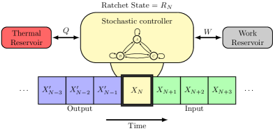
Figure 1: Information engine as a finite-state ratchet (controller) connected to a thermal reservoir, a work reservoir, and an information reservoir (depicted as tape whose storage cells may be read or written).

At each step, $X_{N}$ couples to the ratchet controller for an interaction of duration $\tau$. During this time, thermal fluctuations continuously drive transitions in the coupled state space $\mathcal{R}\times\mathcal{X}$ of the ratchet and the current tape symbol. After the interaction interval, the ratchet is in a potentially different state $R_{N+1}$, and the symbol $X_{N}$ has been transduced into an output symbol $X^{\prime}_{N}=x^{\prime}_{N}\in\mathcal{X}$, which is written to the tape. The strings of possible output symbols are expressed by the random variable $X^{\prime}_{0:\infty}=X^{\prime}_{0}X^{\prime}_{1}\dots$. The tape moves forward, and the next input symbol $X_{N+1}$ begins its interaction with the ratchet, which now starts in state $R_{N+1}$. The joint transitions between states of the ratchet and bit have energetic consequences, capturing energy flows between the thermal and work reservoirs.

II.1 Energetics

These information engines are autonomous and transitions in the coupled ratchet-symbol system are driven by fluctuations in the thermal reservoir. Recently, Ref. [8] introduced a general formalism for determining the energetics of such information engines. First, noting that the ratchet-symbol system obeys detailed balance, transitions over the joint ratchet-symbol state space $\mathcal{R}\times\mathcal{X}$ is described by a Markov chain $M$, where every transition with positive probability—denoted:

$$M_{r_{N}\otimes x_{N}\to r_{N+1}\otimes x^{\prime}_{N}}=$$

$$\>\>\>\Pr(R_{N+1}=r_{N+1},X^{\prime}_{N}=x^{\prime}_{N}|R_{N}=r_{N},X_{N}=x_{N})$$

—must have a reverse transition with positive probability. Energy changes associated with an internal-state transition are then determined by the forward-reverse transition probability ratio:

$$\Delta E_{r_{N}\otimes x_{N}\to r_{N+1}\otimes x^{\prime}_{N}}=k_{\text{B}}T\ln\frac{M_{r_{N+1}\otimes x^{\prime}_{N}\to r_{N}\otimes x_{N}}}{M_{r_{N}\otimes x_{N}\to r_{N+1}\otimes x^{\prime}_{N}}}~{}.$$

Assuming that all energy exchanges with the heat reservoir occur during the ratchet-symbol interaction interval $\tau$ and that all energy exchanges with the work reservoir occur between interaction intervals, the average asymptotic work is:

$$\langle W\rangle=\sum_{r,r^{\prime}\in\mathcal{R},x,x^{\prime}\in\mathcal{X}}\pi_{r\otimes x}M_{r\otimes x\to r^{\prime}\otimes x^{\prime}}\Delta E_{r\otimes x\to r^{\prime}\otimes x^{\prime}}~{},$$ (1)

where $\pi_{r\otimes x}$ is the asymptotic distribution over the joint state of the ratchet-symbol system at the beginning of an interaction interval.

II.2 Structure

To discuss the computational structure of information engines, we first cast the input and output strings in terms of the hidden Markov Models (HMMs) that generate them.

Definition 1.

A finite-state edge-labeled hidden Markov model (HMM) consists of:

1. A finite set of states $\bm{\mathcal{S}}=\{\sigma_{1},...,\sigma_{N}\}$,

2. A finite alphabet $\mathcal{A}$ of $k$ symbols ${x}\in\mathcal{A}$, and

3. A set of $N$ by $N$ symbol-labeled transition matrices $T^{({x})}$, ${x}\in\mathcal{A}$: $T^{({x})}_{ij}=\Pr(\sigma_{j},{x}|\sigma_{i})$. The corresponding overall state-to-state transitions are described by the row-stochastic matrix $T=\sum_{{x}\in\mathcal{A}}T^{({x})}$.

This information-ratchet representation allows us to consider the internal states $\mathcal{S}$ of the input machine (HMM) as well as the internal states $\mathcal{S}^{\prime}$ of the output machine (HMM). The latter are the joint states of the input process and the ratchet: $\mathcal{S}^{\prime}=\mathcal{S}\times\mathcal{R}$.

When the string of inputs or outputs can be generated by an HMM with only a single internal state, they are memoryless, since they can store no information from the past. The random variables generated by the associated HMM are independent and identically distributed (IID). When there is more than a single state, in contrast, the associated process is memoryful and the random variables generated may be correlated in time.

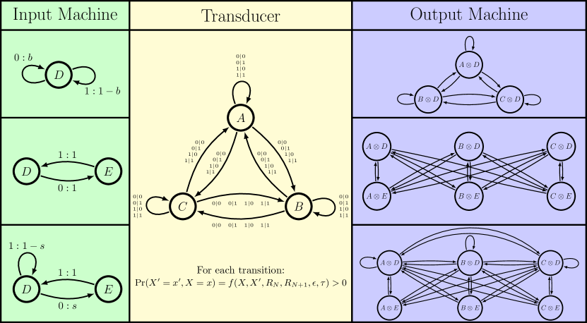
Figure 2: Composing the Mandal-Jarzynski transducer (center, yellow) with a Hidden Markov model (left, green) that describes the process on the input tape gives an output Hidden Markov model (right, purple) that describes the process written to the output tape. Hidden Markov model (HMM) states $R$ are depicted as circles. Directed edges between states represent possible transitions on an observed symbol ${x}$. HMM edges are labeled ${x}:\Pr({x}^{\prime},R_{N+1}|R_{N})$. Transducers are similarly depicted by circular states with directed edges representing possible transitions on pairs of input symbols ${x}$ and output symbols ${x}^{\prime}$. Transducer transitions are specified by ${x}^{\prime}|{x}:\Pr({x}^{\prime},R_{N+1}|{x}^{\prime},R_{N})$. Left: Input HMMs discussed here, from top to bottom, a (memoryless) Biased Coin, a Period-2 Process, and the Golden Mean Process. Center: The Mandal-Jarzynski ratchet, represented by a three-state transducer. Probabilities are not shown on edge labels for conciseness, but are nonzero for all transitions and all combinations of input-output symbol pairs $({x},{x}^{\prime})$. Each edge probability is a function—denoted by $f(\ldots)$—of the previous state $R_{N}$, the next state $R_{N+1}$, the input symbol ${x}$, and the output symbol ${x}^{\prime}$. See Section IV and Appendix B for further details. Right: Output HMMs resulting in the Mandal-Jarzynski transducer composed with the corresponding input HMM on left. Edge labels are left off for conciseness, but each transition label represents a positive probability of observing a $0$ or a $1$.

Similarly, we cast the ratchet controller as a transducer that maps from input sequences to distributions over output sequences.

Definition 2.

A finite-state edge-labeled transducer consists of:

1. A finite set of states $\mathcal{R}=\{R_{1},...,R_{N^{\prime}}\}$,

2. A finite input alphabet $\mathcal{A}$ of $k$ symbols ${x}\in\mathcal{A}$,

3. A finite output alphabet $\mathcal{A}^{\prime}$ of $k^{\prime}$ symbols ${x}^{\prime}\in\mathcal{A}^{\prime}$, and,

4. A set of $N^{\prime}$ by $N^{\prime}$ input-output symbol-labeled transition matrices $T^{({x},{x}^{\prime})}$, ${x},{x}^{\prime}\in\mathcal{A}\times\mathcal{A}^{\prime}$:

   $$T^{({x},{x}^{\prime})}_{ij}=\Pr(r_{j},{x}^{\prime}|r_{i},{x})~{}.$$

The transducer formulation allows us to calculate the output HMM in terms of the ratchet and the input machine. The exact method is given in Section B.1. As with the input machine, a ratchet is memoryless when it possesses only one internal state, and memoryful otherwise. A key feature of a ratchet we focus on here is its ability to alter temporal correlations by altering the structure of an input process. If memoryless (IID) input is fed to a memoryful ratchet, generally the output will be memoryful, since this guarantees the state space dimension of the output $|\mathcal{R}^{\prime}|=|\mathcal{S}\times\mathcal{R}|>1$. Figure 2 graphically illustrates the composition of various input process HMMs with the ratchet transducer we analyze in detail shortly.

II.3 Informatics

Following Landauer, extensions of the Second Law of Thermodynamics were proposed to bound the thermodynamic costs of information processing by an information engine. Reference [6] employed a bound that compares the Shannon entropy of single input and single output symbols. Recall that the Shannon entropy $H_{1}$ for a single random variable $X$ realizing values $x\in\mathcal{X}$ is:

$$H_{1}[X]=-\sum_{x\in\mathcal{X}}\Pr(X=x)\log_{2}\Pr(X=x)~{}.$$ (2)

This Shannon entropy quantifies the randomness of the single random variable $X$ averaged over time. That is, $H_{1}[X]$ answers the question of how uncertain it is that any particular $x_{N}$ will be $0,1,\ldots,$ or $k-1$.

Comparing the single-symbol Shannon entropy in the input string to that in the output string quantifies how the ratchet transforms randomness in individual symbols. This difference captures one aspect of the ratchet’s information processing. And, it was proposed as an upper bound on the asymptotic work done $\langle W\rangle$ [6]:

$$\langle W\rangle \stackrel{{\scriptstyle?}}{{\leq}}k_{\text{B}}T\Delta H_{1}~{},$$ (3)

where $H_{1}=H_{1}[X]$ is the entropy averaged over the input tape, $H_{1}^{\prime}=H_{1}[X^{\prime}]$ is that averaged over the output, and $\Delta H_{1}=H_{1}^{\prime}-H_{1}$ is the change in the single-symbol statistics produced by the ratchet’s operation.

Note, however, that while the $H_{1}$s track the average information in any single instance of $X_{t}$ or $X^{\prime}_{t}$, they do not account for temporal correlations within input sequences or within output sequences. This is key, as information ratchets change more than the statistical bias in an individual symbol, they alter temporal correlations in symbol strings. These altered correlations are related to the fact that the ratchet induces structural change in its input. Recognizing this is central to bounding the thermodynamic costs of the ratchet’s interaction with the input process.

To properly address how correlations affect costs, we calculate a process’ intrinsic randomness when all temporal correlations are taken into account, as measured by the entropy rate [11]:

$$h_{\mu}=\lim\limits_{\ell\rightarrow\infty}\frac{H(\ell)}{\ell}~{},$$ (4)

where $H(\ell)=\operatorname{H}[\Pr({X}_{0:\ell-1})]$ is the Shannon entropy for length-$\ell$ symbol blocks.

Replacing the input and output Shannon entropies in Eq. (3) with their respective entropy rates gives the Information Processing Second Law (IPSL) [7]:

$$\langle W\rangle \leq k_{\text{B}}T\ln 2\left(h_{\mu}^{\prime}-h_{\mu}\right)$$

$$=k_{\text{B}}T\ln 2~{}\Delta h_{\mu}~{}.$$ (5)

The IPSL correctly expresses the upper bound on work, taking into account the presence of temporal correlations in input and output processes.

The importance of Eq. 5 cannot be overstated—any memoryful ratchet induces temporal correlations in its output, even for IID input. Using Eq. 3 in the IID case typically overestimates the upper limit on available work. Additionally, temporal correlations in the input are known to be a thermodynamic resource [12]. In fact, suitably designed ratchets can leverage such correlation to do useful work. Thus, inappropriately applying Eq. 3 in these cases often results in claims that violate the Second Law. In short, Eq. 5 generalizes Landauer’s Principle to the case of correlated environments and finite-state memoryful ratchets that generate correlated outputs.

Unfortunately, due to the difficulty of accurately calculating the entropy rate for most processes, previous treatments of information ratchets were restricted to use either Eq. 3 or finite-length approximations to Eq. 5. Here, we make use of a novel solution that removes this restriction and gives accurate calculations of entropy rates for processes generated by general HMMs.

III Entropy Rate of HMMs

Properly determining the entropy rate of processes generated by HMMs is a longstanding challenge, one known since the 1950s [13]. Its recent resolution required introducing new concepts from ergodic theory and dynamical systems [14]. We now turn to briefly discuss these and the new analysis tools that follow from them. (The Supplementary Materials give a more detailed exegesis.)

III.1 $\epsilon$-Machines

First, though, we need to more carefully consider the hidden Markov models that we use to represent stochastic processes. We briefly recall two important HMM classes.

Definition 3.

A unifilar HMM (uHMM) is an HMM such that for each state $\sigma_{k}\in\bm{\mathcal{S}}$ and each symbol ${x}\in\mathcal{A}$ there is at most one outgoing edge from state $\sigma_{k}$ labeled with symbol ${x}$.

This seemingly-minor structural property means that the states are predictive: current state and symbol exactly predict the next state. This has important consequences for calculating the statistical and informational properties of the process that an HMM generates. If an HMM is unifilar, we may directly calculate the entropy of its generated process via the closed-form expression:

$$h_{\mu}=-\sum_{\sigma\in\bm{\mathcal{S}}}\Pr(\sigma)\sum_{\sigma^{\prime}\in\bm{\mathcal{S}},{x}\in\mathcal{A}}T_{\sigma\sigma^{\prime}}^{({x})}\log_{2}T_{\sigma\sigma^{\prime}}^{({x})}~{}.$$ (6)

In contrast, if an HMM is nonunifilar, its states are not predictive and there is no closed form for the generated process’ entropy rate.

Definition 4.

An $\epsilon$-machine is a uHMM with probabilistically distinct states: For each pair of distinct states $\sigma_{k},\sigma_{j}\in\bm{\mathcal{S}}$ there exists some finite word $w={x}_{0:\ell-1}$ such that:

$$\Pr({X}_{0:\ell}=w|\mathcal{S}_{0}=\sigma_{k})\not=\Pr({X}_{0:\ell}=w|\mathcal{S}_{0}=\sigma_{j})~{}.$$

As a consequence, a process’ $\epsilon$-machine is its optimally-predictive model [15]. Moreover, a process’ $\epsilon$-machine is minimal and unique. This means that we can quantify the amount of structural memory a process effectively uses by counting the number of states in its $\epsilon$-machine or by calculating its stored information. The latter is the statistical complexity $C_{\mu}$, which is the Shannon entropy of the asymptotic probability distribution over states:

$$C_{\mu} =\operatorname{H}[\Pr(\mathcal{S})]$$

$$=-\sum_{\sigma\in\mathcal{S}}\Pr(\sigma)\log_{2}\Pr(\sigma)~{}.$$ (7)

So, knowing a process’ $\epsilon$-machine is powerful, as it provides closed-form expressions for both a process’ intrinsic randomness and its structural memory [16], two important thermodynamic resources.

That said, even if a ratchet’s input is generated by a finite $\epsilon$-machine, the output process will not be. In general, the output process generator (Fig. 2, right column) will be a nonunifilar HMM. This precludes a direct calculation of the entropy rate of a ratchet’s output process. And so, when determining thermodynamic function, it appears that a key constituent ($h_{\mu}^{\prime}$) is inaccessible. Note, too, that nonunifilarity precludes determining the output process’ memory $C_{\mu}^{{}^{\prime}}$ and, failing that, one cannot accurately analyze the changes in structure effected by a ratchet.

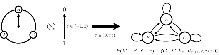
Figure 3: Ratchet schematic adapted from the original Mandal-Jarzynski construction, showing how the dial-and-symbol system is transformed into a three state transducer upon selection of a specific $\epsilon$—determining the energetics of flipping a bit—and $\tau$—determining the interaction interval. For almost every value of $\epsilon$ and $\tau$ every state-to-state transition has positive probability for every input-output symbol combination.

III.2 Mixed-State Presentation

Despite there being no closed-form expression for the entropy rate of the process generated by a finite nonunifilar HMM, there is a way to unifilarize HMMs, introduced by Blackwell [13], using mixed states. A mixed state is the answer to the question: “given that one knows the HMM structure (states and transitions) and has observed a particular sequence, what is the best guess of the internal state probabilities?” More formally, an $N$-state HMM’s mixed states are conditional probability distributions $\eta({x}_{-\ell:0})=\Pr(\mathcal{R}_{0}|{X}_{-\ell:0}={x}_{-\ell:0}$) over the HMM’s internal states $\mathcal{R}$, given all sequences ${x}_{-\ell:0}\in\mathcal{A}^{\ell}$, $\ell=0,1,2,\ldots$.

The collection of mixed states over all of a process’ allowed sequences, i.e., $\ell\to\infty$, induces a (Blackwell) measure $\mu$ on the state distribution $\Pr(\mathcal{R})$ $(N-1)$-dimensional simplex $\bm{\mathcal{R}}$. The mixed states together with the mixed-state transition dynamic (see SM Section A.3) give an HMM’s mixed-state presentation (MSP).

The MSP is unifilar by construction. However, in the typical case, this improvement comes at a heavy cost—the set of mixed states is uncountably infinite. This renders the complexity-measure expressions Eq. 6 and Eq. 7 unusable. Blackwell provided a formal replacement for Eq. 6’s entropy-rate expression [13]. This is an integral expression for the entropy rate over the invariant Blackwell measure $\mu(\eta)$ in the mixed-state simplex $\bm{\mathcal{R}}$:

$$h^{B}_{\mu}=-\int_{\bm{\mathcal{R}}}d\mu(\eta)\sum_{x\in\mathcal{A}}\Pr(x|\eta)\log_{2}\Pr(x|\eta)~{}.$$ (8)

Recently, Ref. [14] introduced a constructive approach to evaluate this integral by establishing contractivity of the simplex maps—the substochastic transition matrices of Def. 1—by showing that the mixed-state process is ergodic. Given this, rather than integrate over the measure $\mu(\eta)$ as required by Blackwell’s Eq. (8), we can then time-average over the series $\eta_{0},\eta_{1},\ldots,\eta_{t}$ of iterated mixed states to obtain the entropy rate:

$$\widehat{h_{\mu}^{B}}=-\lim_{\ell\to\infty}\frac{1}{\ell}\sum_{t=0}^{\ell}\sum_{{x}\in\mathcal{A}}\Pr({x}|\eta_{\ell})\log_{2}\Pr({x}|\eta_{\ell})~{},$$ (9)

where $\Pr({x}|\eta_{\ell})=\eta({x}_{0:\ell})\cdot T^{({x})}\cdot{\mathbf{1}}$, ${x}_{0:\ell}$ is the first $\ell$ symbols of an arbitrarily long sequence ${x}_{0:\infty}$ generated by the mixed-state process, and ${\mathbf{1}}$ is a column-vector of all $1$s. (See SM Section A.3.) Applying Eq. 9 in the present setting means we can now calculate the entropy rate of output processes for arbitrary ratchets and arbitrary inputs.

Characterizing a nonunifilar HMM’s structure is slightly more delicate. Due to the generic uncountability of predictive states for nonunfilar HMMs, $C_{\mu}$ of the set of mixed states diverges. To characterize the divergent memory resource cost of predicting processes with uncountably infinite mixed states, we track the rate of divergence of $C_{\mu}$—the statistical complexity dimension $d_{\mu}$ of the Blackwell measure $\mu$ on $\bm{\mathcal{R}}$ [17]:

$$d_{\mu}=\lim_{\varepsilon\to 0}-\frac{\operatorname{H}_{\varepsilon}[\mathcal{R}]}{\log_{2}\varepsilon}~{},$$ (10)

where $\operatorname{H}_{\varepsilon}[Q]$ is the Shannon entropy of a continuous-valued random variable $Q$, coarse-grained at size $\varepsilon$, and $\mathcal{R}$ is the random variable associated with the mixed states $\eta\in\bm{\mathcal{R}}$. SM Section A.3 develops an upper bound on this that can be accurately determined from the measured process’ entropy rate $\widehat{h_{\mu}^{B}}$ (Eq. 9) and the mixed-state process’ Lyapunov characteristic exponent spectrum $\Lambda$. As discussed in SM A.5, this upper bound is a close approximation to $d_{\mu}$ for broad classes of HMMs, but may be a strict inequality for others.

In this way, the functional thermodynamics of finite-state Maxwellian ratchets can be accurately determined and systematically explored.

IV Mandal-Jarzynski Information Ratchet

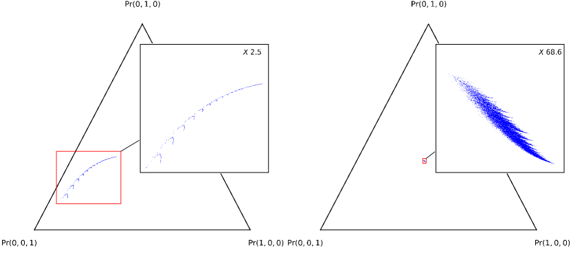
Figure 4: Mixed states $\eta\in\bm{\mathcal{R}}$ of the output process generated by the ratchet driven with memoryless input (Fig. 2(top row)) plotted on the $2$-simplex. Corner labels give the mixed-state probability distributions $\eta=\left(\Pr(A\otimes D),\Pr(B\otimes D),\Pr(C\otimes D)\right)$. Mixed states at the simplex corners correspond to the HMM being in exactly one of its states, while mixed states in the simplex interior are mixtures of the possible HMM states, with $\eta=\left(\frac{1}{3},\frac{1}{3},\frac{1}{3}\right)$ lying at the center. (Left) Ratchet parameters $\delta=-0.98$, $\epsilon=0.01$, and $\tau=0.1$. (Right) Ratchet parameters $\delta=0.4$, $\epsilon=0.5$, and $\tau=0.1$. Insets: Detail of the mixed-state sets, magnified by amount indicated in upper right corner.

To demonstrate the descriptive power of these dynamical-thermodynamic results on ratchet entropy, dimension, mixed states, and function, we apply them to a well-known example of an information engine—the Mandal-Jarzynski ratchet [6]; hereafter, the ratchet. Although initially introduced without reference to HMMs and transducers, following Ref. [7] we translate the original ratchet model into the HMM-transducer formalism outlined in Section II. In these terms, the ratchet is a three-state, fully connected transducer, designed such that only transitions that flip an incoming symbol are energetically consequential. As shown in Fig. 3, the ratchet’s transition probabilities are parametrized by $\tau\in\left[0,\infty\right)$—duration of the ratchet-symbol interaction—and $\epsilon\in\left(-1,1\right)$—the weight parameter. For a given $\tau$ and $\epsilon$, the Mandal-Jarzynski model may be written down as the three-state transducer shown in the center column Fig. 2. See SM Appendix B for how to calculate the transducer, which is based on a rate-transition matrix, and SM Section B.1 for the input-transducer composition method.

Any interaction interval in which the input symbol is unchanged is energetically neutral. Therefore, we measure the average work done by the ratchet by the difference in the probability of reading a $1$ on the input tape cell versus writing a $1$ to the output tape cell:

$$\langle W\rangle=k_{\text{B}}T~{}w\left(\Pr(X^{\prime}=1)-\Pr(X=1)\right)~{},$$

where $w(\epsilon)=\log((1+\epsilon)/(1-\epsilon))$. When $\epsilon=0$, flips $0\to 1$ and $1\to 0$ are both energetically neutral; when $\epsilon\to\pm 1$, symbol flips in one direction are energetically favored over the other. Note that this computation finds the same asymptotic work production as Eq. 1; recalled here as an aid to intuition.

Reference [6]’s initial analysis considered only uncorrelated inputs. That is, their input machine was a single-state HMM—a biased coin, with bias $\delta=\Pr(0)-\Pr(1)$. To identify their ratchet’s thermodynamic functionality, the work bound was approximated via Eq. 3—that is, assuming tape symbols were statistically independent. However, the ratchet is memoryful (due to its three internal states) and, therefore, in general induces correlations in its output, even for uncorrelated inputs. Since the single-symbol entropy only upper-bounds the true Shannon entropy rate—$h_{\mu}\leq H_{1}$—Eq. 3 is suspect when used to identify actual thermodynamic functioning. Using new results here, the following shows that, while approximately correct for uncorrelated input, the single-symbol entropy bound is violated for correlated input. Its incorrect use mischaracterizes thermodynamic functioning and can lead to violations of the Second Law.

In addition, our new methods give insight into how the ratchet processes structural information. Due to its inherent nonunifilarity, even when driven by a finite-state $\epsilon$-machine, the ratchet produces nonunifilar output machines that generate processes with an uncountably-infinite set of mixed states, as Fig. 4 shows. Moreover, the figure also demonstrates that as ratchet parameters vary the mixed-state sets have strikingly different structure.

Previous interpretations of ratchet thermodynamic functioning were limited to considering only transformations of randomness; i.e., for given ratchet parameters and input, what is the sign and magnitude of $k_{B}T\ln 2~{}\Delta h_{\mu}$ and how does this affect $\langle W\rangle$? Such questions ignore the key second dimension of information processing illustrated so vividly by Fig. 4. That is, given the same ratchet, parameters, and input, what is the sign and magnitude of $\Delta C_{\mu}$ and $\Delta d_{\mu}$? Does the ratchet construct new patterns in its output ($\Delta C_{\mu}>0$ or $\Delta d_{\mu}>0$) or deconstruct patterns passed to it from the input ($\Delta C_{\mu}<0$ or $\Delta d_{\mu}<0$)? How do these then affect $\langle W\rangle$? Answering structural questions requires a more thorough taxonomy of thermodynamic functionality than the original engine/dud/eraser categories.

V Randomizing and Derandomizing Behaviors

The ratchet’s previously-identified thermodynamic functions engine, eraser, and dud were identified by comparing the sign and magnitude of $k_{B}T\ln 2~{}\Delta h_{\mu}$ to the asymptotic work production. As such, there are three physically possible orderings:

• Engine: $0<\langle W\rangle\leq k_{B}T\ln 2~{}\Delta h_{\mu}$;

• Eraser: $\langle W\rangle\leq k_{B}T\ln 2~{}\Delta h_{\mu}<0$; and

• Dud: $\langle W\rangle\leq 0\leq k_{B}T\ln 2~{}\Delta h_{\mu}$.

A ratchet randomizing inputs ($\Delta h_{\mu}>0$) can operate as an engine, if it is leveraging the change in entropy rate to do useful work. It may also act as a dud, if the randomization produces no useful work or, worse, if the ratchet is using work. A ratchet derandomizing inputs ($\Delta h_{\mu}<0$) is termed an “eraser” and can only derandomize up to $\langle W\rangle/k_{B}T\ln 2$ bits using $\langle W\rangle$ joules of work. The ordering $k_{B}T\ln 2~{}\Delta h_{\mu}<\langle W\rangle<0$ would imply that the ratchet is derandomizing beyond the physical limitations of Landauer’s principle.

As noted already, Ref. [6] originally identified these functionalities using the entropy-change approximation $\Delta H_{1}$ rather than the exact change $\Delta h_{\mu}$ introduced by Ref. [7]. As previously shown, driving a memoryful ratchet with a memoryful input violates Eq. 3 [12]. In all other cases, Eq. 3 is valid, but may mischaracterize the functional thermodynamic regimes. A natural question, therefore, is how much difference does using the correct entropy rate make in identifying function? To see this, we now compare $\Delta h_{\mu}$ and $\Delta H_{1}$.

There are three possibilities. First, $\Delta H(1)=\Delta h_{\mu}$. In this case, a ratchet does not change the presence of temporal correlations. This occurs when a memoryless ratchet is driven by memoryless input.

Second, $\Delta H(1)>\Delta h_{\mu}$. Here, a ratchet reduces the presence of temporal correlations, which occurs when a memoryless ratchet has been driven by memoryful input. In this regime, the difference in single-symbol entropy is a tighter bound on the correlation change than the difference in entropy rate. Critical to this case, though, recall that our goal is not a tight bound, but rather an accurate measurement of the gap between information processing and asymptotic work. The upshot is that using Eq. 3 in this case may mischaracterize thermodynamic functionality.

Finally, $\Delta H(1)<\Delta h_{\mu}$, which occurs when a memoryful ratchet is driven by memoryless input. In this case, the ratchet increases temporal correlations in the output, so that the difference in entropy rates is a tighter bound on the asymptotic work production. This is the scenario in the first treatment of the Mandel-Jarzynski ratchet [6]. Note that when a memoryful ratchet is driven with memoryful input, the most generic case, all orderings of $\Delta h_{\mu}$ and $\Delta H(1)$ are possible.

Let’s now turn to consider in detail how the ratchet operates in three distinct environments: Memoryless, periodic, and memoryful inputs. This gives more direct insight into the ratchet’s transformational capabilities.

V.1 Memoryless Input

When the ratchet is driven with a memoryless input, as in the original analysis, Eq. 3 is valid, but IPSL always offers a tighter or equal bound on work production than the single-symbol entropy approximation. This holds since the input is memoryless, while the three-state output machine is memoryful and nonunifilar for almost every parameter setting. As such, one cannot calculate the entropy rate $h_{\mu}^{\prime}$ in closed form. However, the new techniques above can determine the mixed-state presentations of the output HMMs and this gives accurate numerical calculation of both the single-symbol and the IPSL work bounds.

Figure 5: Asymptotic work production $\langle W\rangle$, single-symbol $\Delta H_{1}$ bound, and Kolmogorov-Sinai-Shannon $\Delta h_{\mu}$ bound when ratchet is driven by period-2 memoryful input. Since the input has no parameters, the parameter sweeps only over $\epsilon$ with $\tau=10$.

This all being said, for most parameter values of the Mandal-Jarzynski ratchet, in practice we find that $\Delta h_{\mu}\approx\Delta H_{1}$. In other words, when driven with a memoryless input, the ratchet’s functional thermodynamic regions are not significantly changed when identified via the single-symbol entropy—a minor quantitative difference without a functional distinction. (See Fig. S1 for a comparison of the functional thermodynamic regions found by each bound.) Exploring output-machine MSPs shows this arises from the ratchet’s transition topology. As shown in the middle column of Fig. 2, the ratchet’s transducer is fully connected, and all transitions to any other state on any combination of symbols are possible. Therefore, it is impossible to be certain about which state the ratchet is in; or, indeed, to even be sure which states the ratchet is not in. Graphically, this is represented by the fact that the output-machine mixed states $\eta$ always lie deep in the simplex $\bm{\mathcal{R}}$’s interior, as illustrated in Fig. 4 (Right).

Mixed states lying at $\bm{\mathcal{R}}$’s center correspond to an equal belief in each of the output HMM’s three states: $A\otimes D$, $B\otimes D$, and $C\otimes D$. While those on $\bm{\mathcal{R}}$’s border indicate certainty of not being in at least one state. Since the probability distribution over the next symbol is a continuous function over the mixed states (see Section A.3), the diameter of the mixed-state set is a rough measure of the presence of temporal correlations in the ratchet’s behavior. To explicitly illustrate this, the mixed states for two example output processes generated by the ratchet are shown in Fig. 4. On the left, the mixed states are spread out, indicating that at the selected parameters, the ratchet induces stronger temporal correlations than in the next example (right). There, all mixed states lie very close together and very near the simplex center. The mixed-state set has very small diameter. For most parameter values, one finds that the mixed states of the memoryless-driven ratchet’s output process cluster closely in the middle of the simplex. (See Fig. S2 for a broader survey of ratchet MSPs for memoryless input.) So, by giving insight into the mixed states of the output process, our new techniques rather directly explain why $\Delta h_{\mu}\approx\Delta H_{1}$.

V.2 Periodic Input

Now, consider driving the ratchet with a periodic input. The Period-$2$ Process, shown in the middle row of Fig. 2, is memoryful, with two internal states. So, it now is possible that Eq. 3 is violated. Since $H_{1}=1$ and $h_{\mu}=0$, the presence of temporal correlations in the input is maximized. Noting this, and the near-memoryless behavior of the ratchet as discussed in Section V.1, we can see that for almost all parameters, the ratchet decreases the presence of temporal correlations in transforming the input process to the output. The periodically-driven ratchet output HMMs have six states and are nonunifilar for nearly all parameter values; see Fig. 2 (middle, last column). And so, we must calculate the these machine’s mixed-state presentations to estimate $h_{\mu}^{\prime}$. Comparing Eq. 3 and Eq. 5 in Fig. 5 to the asymptotic work production shows that Eq. 3 is not violated. As predicted above, it is a tighter bound on $\langle W\rangle$ than Eq. 5.

Although it may seem desirable to use the tighter bound, the single-symbol and entropy rate bounds identify the ratchet’s thermodynamic functioning differently: Since $\langle W\rangle\leq k_{B}T\ln 2~{}\Delta H_{1}\leq 0$ for all values of $\epsilon$, the single-symbol entropy bound classifies the ratchet as an eraser, dissipating work to reduce the randomness in the input. However, when considering temporal correlations, we see that the ratchet is in plain fact a dud—$\Delta h_{\mu}>0$. That is, the ratchet dissipates work while increasing the tape’s intrinsic randomness. This marked mischaracterization of thermodynamic function by the single-symbol entropy highlights an important lesson: Bounding the asymptotic work production as tightly as possible is not the same as correctly identifying the functional thermodynamics. As Ref. [10] recently showed, rather than merely a bound, Eq. 5 is meaningful only when comparing $k_{B}T\ln 2~{}\Delta h_{\mu}$ to $\langle W\rangle$. The difference in the two quantifies the amount of work the ratchet can do, if it were an optimal, globally-integrated information processor. This shows that even when it may appear to outperform Eq. 5, in general Eq. 3 cannot serve as a reliable bound on asymptotic work production. We return to this in our final example, where applying Eq. 3 implies a violation the Second Law.

V.3 Memoryful Input

Figure 6: Functional thermodynamic regions of the ratchet driven with the Golden Mean Process as a function of parameters $\epsilon\in[-1,1]$ and $s\in[-1,1]$ with $\tau=1$. (Left) Purported functionality identified via by single-symbol entropy bound Eq. 3. (Right) Correct functionality identified via the entropy-rate bound IPSL Eq. 5.

Finally, let’s drive the ratchet with a mixed-complexity memoryful process—partly regular, partly stochastic—the Golden Mean Process. As depicted in Fig. 2 (bottom row), this two-state HMM generates a family of processes parametrized by $s\in[0,1]$. When $s=1$, the process is period-$2$. Decreasing $s$ lets the process emit multiple $1$s in a row. This increases in probability until at $s=0$, where the process emits only $1$s. The driven ratchet’s output HMMs have six states and are nonunifilar for nearly all parameter values; see Fig. 2(bottom, last column). So, again, we must calculate mixed-state presentations to get $h_{\mu}^{\prime}$ and identify functionality.

In Fig. 6, we apply both Eq. 3 and Eq. 5 for the same set of ratchet parameters. For both, we find asymmetry in the functional thermodynamic regions with respect to $\epsilon$, in contrast to the highly symmetric regions found for memoryless input, shown in Fig. S1. This is due to the asymmetry in input. In fact, it is not possible for the Golden Mean Process to produce strings biased towards $0$. Thermodynamically, for $\epsilon>0$, the ratchet is not able to extract work. When applying the single-symbol bound, as shown on the left in Fig. 6, the bound reports large regions of eraser behavior. And, most importantly, between the engine and lower eraser region lies a region where we see that Eq. 3 implies

$$\langle W\rangle>k_{B}T\ln 2~{}\Delta H_{1}~{},$$ (11)

a violation of the Second Law!

Of course, when we apply Eq. 5 in Fig. 6 (Right), the violation region disappears, to be correctly identified as duds. Additionally, the large region of eraser functionality in Fig. 6 (Left) shrinks significantly in Fig. 6 (Right). Figure 6 (Left)’s regions have been mischaracterized similar to the case discussed in Section V.2. It is more subtle here, though, since $h_{\mu}>0$. However, the fundamental problem is the same—by considering only the single-symbol entropy, it appears that the ratchet performs work to make the input less random, since $\Delta H_{1}<0$. In fact, the output is more intrinsically random than the input, and the ratchet dissipates work uselessly. In the violation region on the left, the ratchet is identified as not dissipating sufficient work to reduce the randomness as much as $\Delta H_{1}$ implies it must be. This leads to the Second Law violation. This contradiction is resolved when we take into account that the input’s intrinsic randomness was actually much lower than its single-symbol entropy. And so, the apparent decrease in randomness was in fact an increase.

It is already known that Eq. 3 may be violated in cases of a memoryful ratchet driven by memoryful input. However, the Mandal-Jarzynski ratchet was not designed to find such a violation, as has been done previously [8]. Rather, we find that driving a simple transition-rate based ratchet with a mixed-complexity process creates regions of violation when applying Eq. 3. Since such ratchets are common in application, and any such ratchet will be highly stochastic by nature, for reasons further discussed in Appendix B, we conclude that Eq. 3 is not suitable to be broadly applied. On the positive side, we see that the dynamical-systems techniques introduced here apply broadly, giving consistent and accurate characterizations stochastic-control information engines.

VI Constructing and Deconstructing Patterns

Figure 7: After passing through the information engine, the input process, which has some initial $h_{\mu}$ and $d_{\mu}$, is transformed into an output process with a potentially different $h_{\mu}^{\prime}$ and $d_{\mu}^{\prime}$. By carefully selecting input, an information engine can be induced to act as a randomizer ($\Delta h_{\mu}>0$) or derandomizer ($\Delta h_{\mu}<0$) and a pattern constructor ($\Delta d_{\mu}>0$) or deconstructor ($\Delta d_{\mu}<0$). We show here that all four regions of the $\Delta h_{\mu}$–$\Delta d_{\mu}$ plane are accessible to the Mandal-Jarzynski ratchet by carefully selecting parameters and input. The two insets on the left show the uncountable set of mixed states of an input process that the ratchet transduces to an IID output. The insets on the right show two uncountably-infinite-state output processes produced by running the Mandal-Jarzynski ratchet on a biased coin. The parameters, clockwise from top right: $\delta_{input}=-0.98,\epsilon=0.01,\tau=0.1$; $\delta_{input}=0.3,\epsilon=0.5,\tau=0.1$; $\delta_{output}=0.8,\epsilon=-0.96,\tau=0.75$; $\delta_{output}=0.0,\epsilon=0.9,\tau=0.9$.

Up to this point, we monitored how the ratchet changed the amount of intrinsic randomness present in a symbol sequence and leveraged this to do useful work. When information ratchets are memoryful, they can alter not only the statistical bias of a symbol sequence, but also the presence of temporal correlations. This has thermodynamic consequences, as discussed above. Now, we turn to consider by what mechanisms an information ratchet changes the presence of temporal correlations, which manifests in changes in sequence structure and organization.

By structure and organization, we refer the internal states of the HMM that generates the input symbol sequence, the ratchet states and transitions, and the output sequence. As depicted in Fig. 2, the input and the ratchet each have their own set of internal states. Since the output machine is the composition of the ratchet transducer and input HMM, its states are the Cartesian product of the set of input states and set of output states. In the simplest case, when a memoryless ratchet is driven by memoryless input, there is only ever one state, and no temporal correlations are present at any stage. The only possible action of the ratchet then is to change the statistical bias of individual input symbols and transform this change in Shannon entropy to a change in thermodynamic entropy.

When one or both of the input and ratchet are memoryful, the internal structure of the output will be, in general, memoryful. That is, the ratchet has induced a structural change in processing the input to generate the output. Consider two basic structural-change operating modes [10]: pattern construction, where the output is more structured than the input, and pattern deconstruction, the output is less structured. As before, these modalities are input-dependent—the same ratchet may exhibit either. Note that structural change to the symbol sequence does not uniquely determine the thermodynamic functionality associated with changes in randomness. It is possible for an information engine to act as an engine, eraser, or dud while constructing patterns. The same is true of deconstruction. Rather, transformations of randomness and structure are orthogonal, and a ratchet’s information processing capabilities may lie anywhere in the $\Delta h_{\mu}$—$\Delta d_{\mu}$ plane sketched in Fig. 7.

VI.1 Pattern Construction

Ideal pattern construction occurs when a ratchet takes structureless input—an IID process—to structured output. Therefore, when the ratchet is driven with a biased coin input, it is operating as an ideal pattern constructor. As discussed in Section V.1, driving the ratchet with memoryless input results in an uncountably-infinite set of states in the output HMM for most parameter values. The exception occurs along the line $\delta=\epsilon$ in parameter space, where the ratchet returns the input unchanged, implying $\Delta C_{\mu}=0$. At every other point in ratchet parameter space $\Delta C_{\mu}=+\infty$ and the ratchet acts as a pattern constructor. As can be seen from Fig. S1, this type of structural change can be associated with any thermodynamic behavior.

The resulting divergence of $C_{\mu}$ is a direct consequence of the nonunifilarity induced by the ratchet. The structure generated by any ratchet driven by an IID process is the set of mixed states of the ratchet, given knowledge of the outputs. Due to the ratchet’s topology, there is an uncountable infinity of such mixed states. In this circumstance one uses the statistical complexity dimension—$d_{\mu}$ of Eq. 10—of the set of output mixed states to monitor the rate of the memory-resource divergence. $\Delta d_{\mu}$ distinguishes between output machines with an uncountable infinity of states, and so is able to compare the structural information processing of the ratchet across parameter space.

Figure 7 places two examples of ideal pattern construction on the right side of the $\Delta h_{\mu}$–$\Delta d_{\mu}$ plane with the associated input and output machines, the latter plotted on the 2-simplex. Although it may appear that the more entropic ratchet in the upper half of the plane constructs a more “complex” pattern, this is not so. Refer back to Fig. 4 and compare the dimension of the two sets of mixed states to see the opposite is true. The ratchet operating in the $-\Delta h_{\mu}$ half of the plane produces a much denser set of states, resulting in a larger $\Delta d_{\mu}$. In addition to the structural transformation, the ratchet in the $+\Delta h_{\mu}$ plane randomizes inputs as a dud, while the other derandomizes inputs as an eraser.

VI.2 Pattern Deconstruction

In a complementary fashion, the ratchet can deconstruct patterns. In ideal pattern deconstruction, a ratchet transforms a memoryful input sequence, with $C_{\mu}>0$, to memoryless, IID output, with $C_{\mu}=0$. When taking a ratchet-focused view, as we do here, ideal pattern deconstruction is a more involved task than ideal pattern construction, since we must carefully design inputs that a ratchet will transform into a biased coin. Any correlations in the input must be recognizable by the ratchet so that the ratchet can map them to randomness. Similar to the previous discussion, we consider the induced ratchet mixed states, but now we have knowledge of the inputs. The algorithm to design the required input process, given knowledge of the ratchet, is discussed in Section B.4.

Critically, pattern deconstruction is not possible for all ratchet parameters and desired output. That said, the Mandal-Jarzynski ratchet can perform as an engine, eraser, or dud while deconstructing patterns, as can be seen in Fig. S3. As $\tau$ increases, the parameter-space region in which the ratchet can extract patterns shrinks. At $\tau\to\infty$ pattern extraction may only occur along the line $\delta=\epsilon$. In a mirror of pattern construction, generating the input processes require reference to the uncountably infinite set of mixed states of the ratchet. In general, this implies that an input process which maps to a memoryless output process also has an uncountably-infinite set of states and $\Delta C_{\mu}\to-\infty$. In other words, to properly ensure the output symbols are temporally uncorrelated, the input process must remember its infinite past. Once again, the associated statistical complexity dimension $d_{\mu}$—now of the set of input mixed states—quantifies the rate of the memory-resource divergence.

Two examples of ideal pattern deconstruction are placed on the left side of the $\Delta h_{\mu}$–$\Delta d_{\mu}$ plane in Fig. 7, with the ratchet mixed states—on the 2-simplex—and the output machine. $\Delta d_{\mu}$ is approximate, based on the dimension of the ratchet mixed states, which are conjectured to have the same dimension as the input mixed states.

VI.3 Thermodynamic Taxonomy of Construction and Deconstruction

From its highly stochastic nature and from parameter sweeps like the one shown in Fig. S2, we conclude that for almost all parameters, the Mandal-Jarzynski ratchet is only able to construct patterns with infinite sets of predictive features (mixed states). We conjecture that likewise, it is only able to perfectly deconstruct infinite patterns. An interesting note is that the input and output mixed-state sets and their dimensions are asymmetric. We can visually see the asymmetry in Fig. 7, which sketches the $\Delta h_{\mu}$–$\Delta d_{\mu}$ plane and shows an example of the Mandal-Jarzynski ratchet operating in all four quadrants. Infinite state output constructed by the ratchet may span the simplex, but the mixed states of the ratchet, while acting as a deconstructor, always lie along a line in the simplex. This implies that while the ratchet may construct patterns up to $\Delta d_{\mu}=2.0$, it is only able to deconstruct patterns up to $\Delta d_{\mu}=-1.0$. The difference in $\Delta d_{\mu}$ in these two modalities points to a difference in memory-resource divergence for pattern construction versus pattern deconstruction.

This asymmetry is not necessarily surprising. Recall the asymmetry in the the ratchet’s ability to randomize and derandomize behavior. The combined area of dud and engine region in Fig. 6 consists of the ratchet’s randomizing regime, while the derandomizing regime is the comparatively small eraser region. One interpretation of this asymmetry comes from the thermodynamic limitations on the ordering of $\Delta h_{\mu}$ and $\langle W\rangle$: While an increase in $\Delta h_{\mu}$ is thermodynamically unbounded, $\Delta h_{\mu}$ is constrained by the Second Law to only drop as low as the minimum asymptotic work. This strongly suggests that there is a thermodynamic taxonomy of structural transformation—one that parallels our existing thermodynamic taxonomy of randomness transformation. We must leave finding such a taxonomy and the analysis of more general ratchets with input-dependent structural behavior to future work.

VII Related Efforts

We can now place the preceding methods and new results in the context of prior efforts to identify the thermodynamic functioning of information engines. In short, though, having revealed the challenge of exact entropy calculations and the inherent divergence in structural complexity, the new methods appear to call for a substantial re-evaluation of previous claims. We start noting a definitional difference and then turn to more consequential comparisons.

The framework of information reservoirs discussed here differs from alternative approaches to the thermodynamics of information processing, which include: (i) active feedback control by external means, where the thermodynamic account of the Demon’s activities tracks the mutual information between measurement outcomes and system state [18, 19, 20, 21, 22, 23, 24, 25, 26, 27, 28, 29, 30]; (ii) the multipartite framework where, for a set of interacting, stochastic subsystems, the Second Law is expressed via their intrinsic entropy production, correlations among them, and transfer entropy [31, 32, 33, 34]; and (iii) steady-state models that invoke time-scale separation to identify a portion of the overall entropy production as an information current [35, 36]. A unified approach to these perspectives was attempted in Refs. [37, 38, 39].

These differences being called out, Maxwellian demon-like models designed to explore plausible automated mechanisms that do useful work by decreasing the physical entropy, at the expense of positive change in reservoir Shannon information, have been broadly discussed elsewhere [35, 6, 40, 41, 42, 43, 44]. However, these too neglect correlations in the information-bearing components and, in particular, the mechanisms by which those correlations develop over time. In effect, they account for thermodynamic information-processing by replacing the Shannon information of the components as a whole by the sum of the components’ individual Shannon informations. Since the latter is larger than the former [45], using it can lead to either stricter or looser bounds than the correct bound derived from differences in total configurational entropies. Of more concern, though, bounds that ignore correlations can simply be violated. Finally, and just as critically, the bounds refer to configurational entropies, not the intrinsic dynamical entropy over system trajectories—the Kolmogorov-Sinai entropy. A more realistic model was suggested in Ref. [46]. Issues aside, these designs have been extended to enzymatic dynamics [47], stochastic feedback control [48], and quantum information processing [49, 50].

In comparison, our approach expands on that of Ref. [7] that considers a Demon in which all correlations among the system components are addressed and accounted for. As shown above, this has significant impact on the analysis of Demon thermodynamic functionality. To properly account for correlations, we developed a new suite of tools that allow quickly and efficiently analyzing nonunifilar HMMs and related stochastic controllers, which removes the mathematical intractability of analyzing correlations for arbitrary demons. We note that our approach and results are consistent with the analyses that consider the entropy of the system as a whole, therefore treating correlations in the system implicitly, an approach epitomized by Ref. [51]. Since correlations are not ignored, this approach is fully consistent with our treatment. This being said, insofar as that work does not address specific partitioning of the system, it does not offer an explicit accounting of the system’s internal correlations, as is done here. As previously discussed, one may derive information ratchet-type results from that approach by considering an explicit partitioning [12, 10, 52]. While the results are consistent, leaving the role of correlations implicit does not allow for investigating how to best leverage them. It also does not give a way to analyze internal computational structure. These remarks highlight the importance of explicitly considering information engine-style partitioning.

The dynamical-systems methods additionally allowed us to consider a Demon’s internal structure, which had only previously been investigated for unifilar ratchets in Ref. [10]. From engineering and cybernetics to biology and now physics, questions of structure and how an agent, here understood as the ratchet, interacts with and leverages its environment—i.e., input—is a topic of broad interest [53, 54]. General principles for how an agent’s structure must match that of its environment will become essential tools for understanding how to take thermodynamic advantage of correlations in structured environments, whether the correlations are temporal or spatial. Ashby’s Law of Requisite Variety—a controller must have at least the same variety as its input so that the whole system can adapt to and compensate that variety and achieve homeostasis [53]—was an early attempt at such a general principle of regulation and control. For information engines, a controller’s variety should match that of its environment [12]. Above, paralleling this, but somewhat surprisingly, we showed that for the Mandal-Jarzynski ratchet to extract patterns from its environment, the input must have an uncountably infinite set of memory states synchronized to the ratchet’s current mixed state. One cannot but wonder how such requirements manifest physically in adaptive thermodynamic nanoscale devices and biological agents.

VIII Conclusions

Thermodynamic computing has blossomed, of late, into a vibrant and growing research domain, driven by applications and experiment [2, 27, 55, 18, 56, 57, 31, 35, 38, 48, 47, 58, 59, 60, 51]. As such, it is vital that analytical tools accurately relate information processing and thermodynamic functionality. While the original class of Maxwellian information engines was flexible and well suited to specific applications, accurate analysis and correct functional classifications were previously hampered by the challenge of determining the entropy rate of temporally-correlated sequences—sequences that are inevitably induced by Maxwellian ratchets or are present in their possible environments. Previously useful and seemingly reasonable approximations to the entropy rate are not up to this task. As we demonstrated, they can fail miserably—even lead to incorrect attributions of thermodynamic function and, worse, to violations of the Second Law.

Here, we introduced new techniques from dynamical systems and ergodic theory—dimension theory, iterated function systems, and random matrix theory—that overcome these hurdles and, in the process, constructively solve Blackwell’s long-standing question of the entropy rate of processes generated by hidden Markov models. They allow us to accurately determine the thermodynamic functioning of Maxwellian information engines with arbitrary ratchet design, over all possible inputs. In this way, the results significantly expand the set of analyzable engines. In short, this changes the perspective of the current research program from studying highly constrained toy examples to broadly surveying engine designs. This is a boon to both theory, experiment, and engineering.

Furthermore, these tools allowed us to look under the hood, so to speak, and examine more than quantitative changes in the intrinsic randomness of processes, but also to show how ratchets impact structure and correlation. Most strikingly, we showed that, in general, stochastic ratchets generate outputs that require uncountably infinite sets of predictive features to optimally function, even when driven by trivial (temporally uncorrelated) input.

Supplementary Materials
Functional Thermodynamics of Maxwellian Ratchets:
Randomizing and Derandomizing Behaviors,
Constructing and Deconstructing Patterns
Alexandra Jurgens and James P. Crutchfield
arXiv:2003.00139

Appendix A Stochastic Processes

Several of the tools used here come from the theory of classical stochastic processes, we introduce several definitions and notation for the reader less familiar with it. A classical stochastic process $\bf{{X}}$ is a series of random variables and a specification of the probabilities of their realizations. The random variables corresponding to the behaviors are denoted by capital letters $\ldots{X}_{t-2},{X}_{t-1},{X}_{t},{X}_{t+1},{X}_{t+2}\ldots$. Their realizations are denoted by lowercase letters $\ldots{x}_{t-2},{x}_{t-1},{x}_{t},{x}_{t+1},{x}_{t+2}\ldots$, with ${x}_{t}$ values drawn from a discrete alphabet $\mathcal{A}$, in the present setting. Blocks are denoted as: ${X}_{t:t+l}={X}_{t},{X}_{t+1},\ldots{X}_{t+l-1}$, the left index is inclusive and the right one exclusive.

For our purposes, we consider stationary stochastic processes, in which the probability of observing behaviors is time-translation invariant:

$$\Pr(X_{t:t+\ell}=x_{t:t+\ell})=\Pr(X_{0:\ell}=x_{0:\ell})~{},$$

for all $t$ and $\ell$. We consider processes that have finite or infinite Markov order and that can be generated by either finite or infinite hidden Markov models.

A.1 Hidden Markov Models and Unifilarity

A hidden Markov model (HMM) is a quadruple $(\bm{\mathcal{S}},\mathcal{A},\{T^{x}\},\pi)$ consisting of:

• $\bm{\mathcal{S}}$ is the set of hidden states.

• $\mathcal{A}$ the alphabet of symbols that the HMM emits on state-to-state transitions at each time step.

• $\{T^{x}:{x}\in\mathcal{A}\}$ is the set of labeled transition matrices such that $T^{x}_{ij}=\Pr({x},\sigma_{j}|\sigma_{i})$ with $\sigma_{i},\sigma_{j}\in\bm{\mathcal{S}}$. That is, $T^{x}_{ij}$ denotes the probability of the HMM transitioning from state $\sigma_{i}$ to state $\sigma_{j}$ while emitting symbol ${x}$.

• $\pi$ is the stationary state distribution determined from the left eigenvector of $T=\sum_{{x}\in\mathcal{A}}T^{x}$ normalized in probability.

An HMM property that proves to be essential is unifilarity. An HMM is unifilar if, from each hidden state, the emitted symbol ${x}\in\mathcal{A}$ uniquely identifies the next state. Equivalently, for each labeled transition matrix $T^{x}$, there is at most one nonzero entry in each row. Unifilarity ensures that a sequence of emitted symbols has a one-to-finite correspondence with sequences of hidden-state paths.

In contrast, if an HMM is nonunifilar the set of allowed hidden-state state paths corresponding to a sequence of emitted symbols grows exponentially with sequence length. Nonunifilarity makes inferring the underlying states and transitions directly from the generated output process a computationally-challenging task.

A.2 Measures of Complexity

We consider two complexity measures that have clear operational meanings: a process’ intrinsic randomness and the minimal memory resources required to predict its behavior accurately.

The intrinsic randomness of a classical stochastic process $\bf{{X}}$ is measured by its entropy rate [11]:

$$h_{\mu}=\lim\limits_{\ell\rightarrow\infty}\frac{H(\ell)}{\ell}~{},$$ (S1)

where $H(\ell)=\operatorname{H}[\Pr({X}_{0:\ell-1})]$ is the Shannon entropy for length-$\ell$ blocks. That is, a process’ intrinsic randomness is the asymptotic average Shannon entropy per emitted symbol—a process’ entropy growth rate.

Shannon showed that this is the same as the asymptotic value of the entropy of the next symbol conditioned on the past [61]:

$$h_{\mu}=\lim\limits_{\ell\rightarrow\infty}\operatorname{H}[{X}_{0}|{X}_{-\ell:0}]~{}.$$ (S2)

This can be interpreted as how much information is gained per measurement once all the possible structure in the sequence has been captured.

Determining $h_{\mu}$ is possible only for a small subset of stochastic processes. Shannon [61] gave closed-form expressions for processes generated by Markov Chains (MC), which are “unhidden” HMMs—they emit their states as symbols. Making use of Eq. (S2), he proved that for MC-generated processes the entropy rate is simply the average uncertainty in the next state:

$$h_{\mu}=-\sum\limits_{\sigma\in\bm{\mathcal{S}}}\Pr(\sigma)\sum\limits_{\sigma^{\prime}\in\bm{\mathcal{S}}}T_{\sigma\sigma^{\prime}}\log T_{\sigma\sigma^{\prime}}~{},$$ (S3)

where $T$ is the MC’s transition matrix and $\bm{\mathcal{S}}$ its set of states.

Another special case for which the entropy rate can be exactly computed is for processes generated by unifilar HMMs (uHMMs) [11]. This class generates an exponentially larger set of processes than possible from MCs. Since each infinite sequence of emitted symbols corresponds to a unique sequence of internal states, or at most a finite number, the process entropy rate is that of the internal MC. And so, one (slightly) adapts Eq. (S3) to calculate $h_{\mu}$ for these processes. The expression is presented in Eq. (6).

A process’ structure is most directly analyzed by determining its minimal predictive presentation, its $\epsilon$-machine. A simple measure of structure is then given by the number of internal (causal) states $|\bm{\mathcal{S}}|$ or by the statistical complexity $C_{\mu}$ defined in Eq. (7), which is the Shannon information $\operatorname{H}[\bm{\mathcal{S}}]$ stored in the causal states. Since the set of causal states is minimal, $C_{\mu}$ measures of how much memory about the past a process remembers. Said differently, $C_{\mu}$ quantifies the minimum amount of memory necessary to optimally predict the process’ future.

However, for processes generated by nonunifilar HMMs, both $h_{\mu}$ and $C_{\mu}$ given by Eqs. (6) and (7) are incorrect. The former overestimates the generated process’ $h_{\mu}$, since uncertainty in the next symbol is not in direct correspondence with the uncertainty in the next internal state. In fact, there is no exact general method to compute the entropy rate of a process generated by a generic nonunifilar HMM. One has only the formal expression of Eq. (8) which refers to a abstract measure that, until now, was not constructively determined. For related reasons, the statistical complexity $C_{\mu}$ given by Eq. (7) applied to that abstract measure is useless—it simply diverges.

For processes generated by nonunifilar HMMs one can take a very pragmatic approach to estimate randomness and structure from process realizations (measured or simulated time series) using information measures for sequences of finite-length ($\ell$), such as reviewed in Refs. [62, 63]. This approximates the sequence statistics as an order-$\ell$ Markov process. The associated conditional distributions capture only finite-range correlations: $\Pr({X}_{t:\infty}|{x}_{-\infty:t})=\prod_{i=t}^{\infty}\Pr({X}_{i}|{X}_{i-\ell}\ldots{X}_{i-1})$. This approach is data-intensive and the complexity estimators have poor convergence.

Addressing the shortcomings for processes generated by nonunifilar HMMs requires introducing the fundamental concepts of predictive features and a process’ mixed-state presentation.

A.3 Calculating Mixed States

The finite Markov-order approach seems to make sense empirically. However, one would hope that, if we know the nonunfilar HMM and therefore have a model (states and transitions) that generates the process at hand, we can calculate randomness and structure directly from that model. One hopes to at least do better than using slowly-converging order-$\ell$ Markov approximations. The approach is to construct a unifilar HMM—the process’ $\epsilon$-machine—from the nonunfilar HMM. This is done by calculating the latter’s mixed states.

Each mixed state tracks the probability distribution over the the nonunifilar HMM’s internal states, conditioned on the possible sequences of observed symbols. In other words, the mixed states represent states of knowledge of the nonunifilar HMM’s internal states. This also allows one to compute the transition dynamic between mixed states, forming a unifilar model for the same process as generated by the original nonunifilar HMM.

Explicitly, assume that an observer has an HMM presentation $M$ for a process $\mathcal{P}$ and, before making any observations, has probabilistic knowledge of the current state—the state distribution $\eta_{0}=\Pr(\mathcal{S})$. Typically, prior to observing any system output the best guess is $\eta_{0}=\pi$.

Once $M$ generates a length-$\ell$ word $w={x}_{0}{x}_{1}\ldots{x}_{\ell-1}$ the observer’s state of knowledge of $M$’s current state can be updated to $\eta(w)$, that is:

$$\eta_{\sigma}(w) \equiv\Pr(\mathcal{S}_{\ell}=\sigma|{X}_{0:\ell}=w,\mathcal{S}_{0}\sim\pi)~{}.$$ (S4)

The collection of possible states of knowledge $\eta(w)$ form the set $\bm{\mathcal{R}}$ of $M$’s mixed states:

$$\bm{\mathcal{R}}=\{\eta(w):w\in\mathcal{A}^{+},\Pr(w)>0\}~{}.$$

And, we have the mixed-state (Blackwell) measure $\mu(\eta)$—the probability of being in a mixed state:

$$\Pr(\eta(w)) =\Pr(\mathcal{S}_{\ell}|{X}_{0:\ell}=w,\mathcal{S}_{0}\sim\pi)\Pr(w)~{}.$$

From this follows the probability of transitioning from $\eta(w)$ to $\eta(w{x})$ on observing symbol ${x}$:

$$\Pr(\eta(w{x})|\eta(w)) =\Pr({x}|\mathcal{S}_{\ell}\sim\eta(w))~{}.$$

This defines the mixed-state dynamic $\mathcal{W}$ over the mixed states. Together the mixed states and their dynamic give the HMM’s mixed-state presentation (MSP) $\mathcal{U}=\{\bm{\mathcal{R}},\mathcal{W}\}$ [13].

Given an HMM presentation, though, we can explicitly calculate its MSP. The probability of generating symbol ${x}$ when in mixed state $\eta$ is:

$$\Pr({x}|\eta)=\eta\cdot T^{({x})}\cdot{\mathbf{1}}~{},$$ (S5)

with ${\mathbf{1}}$ a column vector of $1$s. Upon seeing symbol ${x}$, the current mixed state $\eta_{t}$ is updated:

$$\eta_{t+1}(x)=\frac{\eta_{t}\cdot T^{({x})}}{\eta_{t}\cdot T^{({x})}\cdot{\mathbf{1}}}~{},$$ (S6)

with $\eta_{0}=\eta(\lambda)=\pi$ and $\lambda$ the null sequence.

Thus, given an HMM presentation we can calculate the mixed state of Eq. (S4) via:

$$\frac{\pi\cdot T^{(w)}}{\pi\cdot T^{(w)}\cdot{\mathbf{1}}}~{}.$$

The mixed-state transition dynamic is then:

$$\Pr(\eta_{t+1},{x}|\eta_{t}) =\Pr({x}|\eta_{t})$$

$$=\eta_{t}\cdot T^{({x})}\cdot{\mathbf{1}}~{},$$

since Eq. (S6) tells us that, by construction, the MSP is unifilar. That is, the next mixed state is a function of the previous and the emitted (observed) symbol.

Transient mixed states are those state distributions after having seen finite-$\ell$ sequences $w$, while recurrent mixed states are those remaining with positive probability in the limit that $\ell\to\infty$. When their set is minimized, recurrent mixed states exactly correspond to causal states $\bm{\mathcal{S}}$ [64].

Now, with a unifilar presentation one is tempted to directly apply Eqs. (6) and (7) to compute measures of randomness and structure, but another challenge prevents this. With a small number of exceptions, the MSP of a process generated by a nonunifilar HMM has an uncountable infinity of states $\eta$ [17]. Practically, this means that one cannot construct the full MSP, that direct application of Eq. (6) to compute the entropy rate is not feasible, and that $|\bm{\mathcal{S}}|$ diverges and, typically, so does $C_{\mu}$.

A.4 Entropy Rate of Nonunifilar Processes

Fortunately, when working with ergodic processes, such as those addressed here, one can accurately estimate the MSP by generating a word $w_{\ell}$ of sufficiently long length [14]. The main text addresses in some detail how to use this to circumvent the complications of uncountable mixed states when computing the entropy rate. Specifically, with the mixed states in hand computationally, accurate numerical estimation of the entropy rate of a process generated by a nonunifilar HMM is given by using the temporal average specified in Eq. (9). The development of that expression is given in Ref. [14].

This handily addresses accurately estimating the entropy rate of nonunifilar processes. And so, we are left to tackle the issue of these process’ structure with the statistical complexity dimension. This requires a deeper discussion.

A.5 Statistical Complexity Dimension

$C_{\mu}$ diverges for processes generated by generic HMMs, as they are typically nonunifilar and that, in turn, leads to an uncountable infinity of mixed states. To quantify these processes’ memory resources one tracks the rate of divergence—the statistical complexity dimension $d_{\mu}$ of the Blackwell measure $\mu$ on $\bm{\mathcal{R}}$:

$$d_{\mu}=\lim_{\varepsilon\to 0}-\frac{\operatorname{H}_{\varepsilon}[\mathcal{R}]}{\log_{2}\varepsilon}~{},$$ (S7)

where $\operatorname{H}_{\varepsilon}[Q]$ is the Shannon entropy (in bits) of the continuous-valued random variable $Q$ coarse-grained at size $\varepsilon$ and $\mathcal{R}$ is the random variable associated with the mixed states $\eta\in\bm{\mathcal{R}}$.

$d_{\mu}$ is determined by the measured process’ entropy rate $\widehat{h_{\mu}^{B}}$, as given by Eq. (9), and the mixed-state process’ spectrum of Lyapunov characteristic exponents (LCEs). The latter is calculated from an HMM’s labeled transition matrices, which map the mixed states $\eta_{t}\in\bm{\mathcal{R}}$ according to Eq. (S6). The LCE spectrum $\Lambda=\{\lambda_{1},\lambda_{2},\ldots,\lambda_{N}:\lambda_{i}\geq\lambda_{i+1}\}$ is determined by time-averaging the contraction rates along the $N$ eigendirections of this map’s Jacobian. The statistical complexity dimension is then bounded by a modified form of the LCE dimension [65]:

$$d_{\mu}\leq d_{\text{LCE}}~{},$$ (S8)

where:

$$d_{\text{LCE}}=k-1+\frac{\widehat{h_{\mu}^{B}}+\sum_{i=1}^{k}\lambda_{i}}{|\lambda_{k+1}|}$$ (S9)

and $k$ is the greatest index for which $\widehat{h_{\mu}^{B}}+\sum_{i=1}^{k}\lambda_{k}>0$. Reference [14] introduces this bound for an HMM’s statistical complexity dimension, interprets the conditions required for its proper use, and explains in fuller detail how to calculate an HMM’s LCE spectrum.

In short, the set of mixed states generated by a generic HMM is equivalent to the Cantor set defining the attractor of a nonlinear, place-dependent iterated function system (IFS). Exactly calculating dimensions—say, $d_{\mu}$—of such sets is known to be difficult. This is why here we adapt $d_{\text{LCE}}$ to iterated function systems. The estimation is conjectured to be accurate in “typical systems” [66, 65, 67]. Even so, in certain cases where the IFS does not meet the open set condition [67]—the relationship becomes an inequality: $d_{\mu}<d_{\text{LCE}}$. This case, which is easily detected from an HMM’s form, is discussed in more detail in Ref. [14].

Appendix B Mandal-Jarzynski Ratchet

To work with the Mandal-Jarzynski ratchet, we reformulated it in computational mechanics terms, which is explained in Section II. In its original conception, the model was imagined as a single symbol (“bit”) interacting with a dial that may smoothly transition between three positions, as shown on the left in Fig. 3. This results in six possible states of the joint dial-symbol system, $\{A\otimes 0,A\otimes 1,B\otimes 0,B\otimes 1,C\otimes 0,C\otimes 1\}$. The transitions among these six states are modeled as a Poisson process, where $\mathcal{R}_{ij}$ is the infinitesimal transition probability from state $j$ to state $i$, with $i;j\in\{A\times 0,\dots,C\times 1\}$ [6]. The weight parameter $\epsilon$, so named because it is intended to model the effect of attaching a mass to the side of the dial, impacts the probability of transitions among the six states by making $0\to 1$ transitions energetically distinct from $1\to 0$ transitions. This creates a preferred “rotational direction”, since bit flips in one direction will be more energetically beneficial than the other. This is what allows the ratchet to do useful work.

Explicitly, the transition rate matrix $\mathcal{R}$ is:

$$\mathcal{R}=\begin{pmatrix}-1&1&0&0&0&0\\ 1&-2&1&0&0&0\\ 0&1&-2+\epsilon&1+\epsilon&0&0\\ 0&0&1-\epsilon&-2-\epsilon&1&0\\ 0&0&0&1&-2&1\\ 0&0&0&0&1&-1\end{pmatrix}~{}.$$ (S10)

To express the ratchet’s evolution over a single interaction interval of length $\tau$, we calculate $\mathcal{T}(\tau,\epsilon)=\left(e^{\mathcal{R}(\epsilon)\tau}\right)^{\intercal}$, the transition matrix of the six-state Markov model representing the Mandal-Jarzynski model. In turn, this six-state model with the states $\{A\otimes 0,A\otimes 1,B\otimes 0,B\otimes 1,C\otimes 0,C\otimes 1\}$ may be transformed into a three-state transducer, with states $\{A,B,C\}$ and input and output symbols in $\{0,1\}$. To do this, we define the projection matrices:

$$\mathbb{P}_{0}=\begin{pmatrix}\mathbb{I}_{3}\\ \mathbf{0}_{3}\end{pmatrix}~{}\text{and}~{}\mathbb{P}_{1}=\begin{pmatrix}\mathbf{0}_{3}\\ \mathbb{I}_{3}\end{pmatrix}~{}.$$

Then, the transducer input-output matrices $K^{\text{in},\text{out}}(\tau,\epsilon)$ for a given $\mathcal{T}(\tau,\epsilon)$ are given by:

$$K^{\text{in},\text{out}}(\tau,\epsilon)=\left(\mathbb{P}_{\text{in}}\right)^{\intercal}\mathcal{T}(\tau,\epsilon)\mathbb{P}_{\text{out}}~{}.$$

For all $\epsilon\in\left(0,1\right)$ and $\tau\in\left(0,\infty\right]$, all four $K^{\text{in},\text{out}}(\tau,\epsilon)$ are positive definite matrices. This is what is meant by “fully-connected, highly stochastic” controller—all transitions on all combinations of symbols have positive probability. Explicitly, the probability function $f(\ldots)$ referenced in both Fig. 2 and Fig. 3 is given by:

$$\Pr(X^{\prime}=x^{\prime},X=x,R_{N}=r,R_{N+1}=r^{\prime}) =f(x,x^{\prime},r,r^{\prime},\epsilon,\tau)$$

$$=\left(\mathbb{P}_{x}\right)^{\intercal}\mathcal{T}_{R,R^{\prime}}(\tau,\epsilon)\mathbb{P}_{x^{\prime}}~{}.$$ (S11)

B.1 Composing a Ratchet with an Input Process’ Machine

Given an input process generated by an HMM with transition matrices $T^{(x)}$, such that $x\in\{0,1\}$, we may exactly calculate the transition matrices $T^{\prime(x^{\prime})}$ of the output HMM:

$$T^{\prime(x^{\prime})}_{R_{N}\times S_{N},R_{N+1}\times S_{N+1}}=\sum_{x}K^{x,x^{\prime}}_{R_{N},R_{N+1}}T^{(x)}_{S_{N},S_{N+1}}~{},$$

noting that the state space of the output HMM is the Cartesian product of the state space of the transducer $\mathcal{R}$ and the state space of the input machine $\mathcal{S}$. Although presenting this in the setting of the Mandal-Jarzynski ratchet specifically, this method applies for any input machine and transducer, given that the transducer is able to recognize the input [68].

That said, there are several interesting points specific to the Mandal-Jarzynski ratchet we should highlight. As noted in the previous section, the Mandal-Jarzynski transducer matrices are positive definite, guaranteeing that the output machine will be nonunifilar, although disallowed state transitions in input machines are preserved in the output. (Composing the Mandal-Jarzynski ratchet with the Golden Mean Process in Fig. 3 illustrates this effect.) This is characteristic of any transducer defined via the rate transition matrix method outlined above. The conclusion is that the techniques required to analyze nonunifilar HMMs are required in general.

B.2 Biased Coin Parameter Sweep

Figure S1: MJ ratchet functional thermodynamic regions over $\epsilon\in[1,-1]$ and $b\in[0,10$ with $\tau=1$. (Left) Purported functionality identified via by single-symbol entropy bound Eq. 3. (Right) Correct functionality identified via the entropy-rate bound IPSL Eq. 5.

As Section V.1 discusses, we recreated the results from Mandal and Jarzynski’s original ratchet [6] using the techniques outlined in this section and in Appendix A. There, the ratchet is driven by a memoryless Biased Coin and the functional thermodynamic regions are identified via Eq. 3 [6]. These results are shown in Fig. S1, on the left, and demonstrate close agreement with the original results. As previously noted, calculating the thermodynamic regions via Eq. 5 did not significantly change the identified regions, as can be seen by comparison to the figure on the right. Although not shown here, we also recreated the results at $\tau=10$, which again show strong agreement with results reported in Ref. [6].

B.3 Information Ratchet Mixed-State Attractor Survey

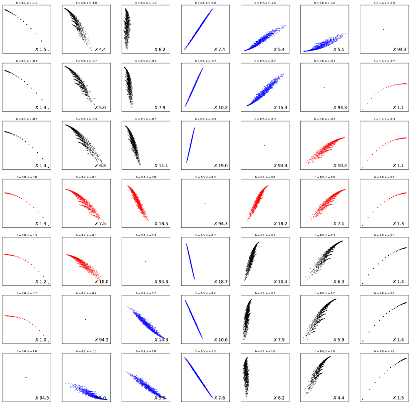
Figure S2: Mixed-state attractors of the output HMMs of the Mandal-Jarzynski ratchet driven by a Biased Coin as a function of $\epsilon$ and input bias $\delta$, given above each square; $(\epsilon,\delta)\in[0,1]\times[-1,1]$. Each plot shows $1,000$ mixed states from the attractor at the magnification noted in the lower right corner. The attractors are color coded according to their thermodynamic functionality, with red being engines, blue representing erasers, and black for duds.

To emphasize how exploring a ratchet’s mixed states elucidates the underlying physics, Fig. S2 presents the attractors of the Mandal-Jarzynski ratchet driven by the Biased Coin, as a function of $\epsilon$ and $b$, in analogy with Fig. S1. Each square in the grid shows the mixed-state attractor for the output HMM produced by the composition of the Mandal-Jarzynski ratchet at the given $\epsilon$ with a Biased Coin at the given bias $\delta$. The grid is laid out identically to the functional thermodynamic plots above, with $\epsilon$ varying on the $y$-axis and the input bias $b$ varying on the $x$-axis. Note that the squares are not at the same scale: each is magnified to show the structure of the attractor; the magnification factor is given in the lower right corner. Compare to Fig. 4 to see the mixed-state attractors in further detail. Additionally, the attractors are color coded to show thermodynamic functionality: red for engines, blue for erasers, and black for duds.

The symmetry of the Mandal-Jarzynski ratchet around $\epsilon=0$ is revealed by how structure of the output HMM attractors is reflected and reversed over the $\epsilon=\delta$ line. Along this diagonal, we see that the mixed-state attractor collapses to a single state—a single point. This reflects the fact that at any $\epsilon=\delta$ the output HMM is the input Biased Coin, so $\langle W\rangle=\Delta H=\Delta h_{\mu}=0$. Furthermore, we see that the structure of the mixed-state attractor does not have a strong effect on the thermodynamic functionality—very similar attractors act as duds and as erasers on each side of the $\epsilon=0$ line. This is as expected since, although thermodynamic functionality appears to change suddenly, the grids in Figs. 6, S1 and S2 actually sweep over output machines with smoothly changing transition probabilities. And, changes in functionality represented by the boundaries of thermodynamic regions are actually due to small, smooth changes in the comparative magnitude of $\langle W\rangle$ and $\Delta h_{\mu}$. Figure S2 illustrates this clearly, as the mixed-state attractor changes smoothly under the parameter sweep.

Note that the construction of Fig. S2 was only possible due to the new dynamical-systems techniques outlined in Sections A.3 and A.4. The recently developed guarantee of ergodicity and quick generation of mixed states allows us to easily plot and investigate the mixed-state attractors of arbitrary HMMs. And, this allows for parameter sweeps of attractors of HMM families and rapid calculation of their entropy rates. The latter was required to determine the thermodynamic functionality color coding in Fig. S2.

B.4 Pattern Deconstruction and Thermodynamic Functionality

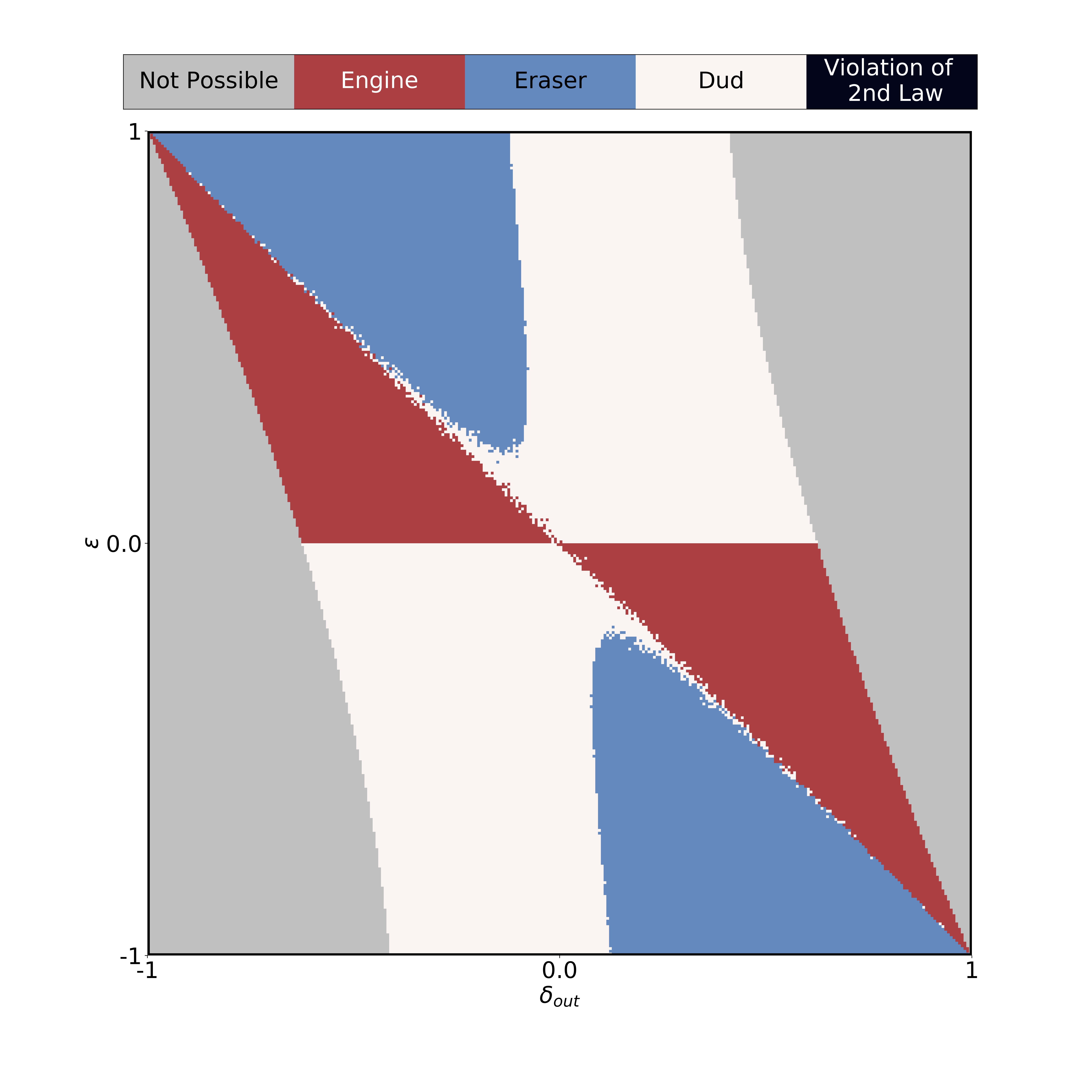
Figure S3: Functional thermodynamic regions of a ratchet pattern deconstructor with an interaction interval of $\tau=0.75$. The $x$-axis sweeps over the output bias $\delta_{out}$, while the $y$-axis sweeps over $\epsilon$. As indicated, there are two parameter regimes where the ratchet is unable to act as a pattern deconstructor. In these regions, the desired output bias is not reachable by the machine at the given $\epsilon$. As $\tau\to\infty$, this region grows, until it encompasses every parameter combination other than $\epsilon=\delta_{out}$, which is always reachable with an input Biased Coin with bias $\delta_{in}=\delta_{out}=\epsilon$.

While it is relatively simple to run the Mandal-Jarzynski ratchet as an ideal pattern constructor, forcing the ratchet to perfectly deconstruct patterns is a more difficult task. As previously discussed in Ref. [10], in order to deconstruct patterns, the input and ratchet must remain synchronized. However, the Mandel-Jarzynski ratchet, being highly stochastic, resists synchronization. Since the input process cannot stay synced to the states of the Mandal-Jarzynski ratchet, it must synchronize to the mixed states instead. To design an input sequence that the ratchet transduces to an IID output process with bias $\delta$ we calculate as follows:

1. Pick a ratchet mixed state;

2. Determine the input-output probability distribution;

3. Calculate the input probability distribution such that $\Pr(X^{\prime}=0)-\Pr(X^{\prime}=1)=\delta$.

4. Step forward, record the input.

5. Use the input to update the ratchet mixed state; and

6. Repeat the procedure starting at Step (1), using the new mixed state.

Note that one must ensure that the output probability distribution remains constant at each time step.

As might be suspected from the algorithm, this is not possible at all parameters. For example, the ratchet may be so heavily biased to flip $0\to 1$ that emitting a sequence of mainly $1$s is mathematically impossible. This is expressed in the algorithm by finding a required input probability distribution with a negative component. This is illustrated in Fig. S3, where the functional thermodynamic regions associated with the Mandal-Jarzynski ratchet acting as a pattern deconstructor are shown. There are two inaccessible regions, where the desired output is not possible for the ratchet at the given value of $\epsilon$. As $\tau\to\infty$ these regions grow in size, until at large $\tau$ the only parameter region capable of pattern deconstruction is $\delta=\epsilon$. This is where the ratchet becomes memoryless, so it is trivially a pattern deconstructor along this line.

References

- [1] J. C. Maxwell. Theory of Heat. Longmans, Green and Co., London, United Kingdom, ninth edition, 1888.
- [2] K. Maruyama, F. Nori, and V. Vedral. Colloquium: The physics of Maxwell’s demon and information. Rev. Mod. Phys., 81, 2009.
- [3] O. Penrose. Foundations of Statistical Mechanics; A Deductive Treatment. Oxford: Pergamon, 1970.
- [4] C. H. Bennet. Thermodynamics of computation—-a review. Int. J. Theor. Phys., 21, 1982.
- [5] R. Landauer. Irreversibility and heat generation in the computing process. IBM J. Res. Develop., 5(3):183–191, 1961.
- [6] D. Mandal and C. Jarzynski. Work and information processing in a solvable model of Maxwell’s demon. Proc. Natl. Acad. Sci. USA, 109(29):11641–11645, 2012.
- [7] A. B. Boyd, D. Mandal, and J. P. Crutchfield. Identifying functional thermodynamics in autonomous Maxwellian ratchets. New J. Physics, 18:023049, 2016.
- [8] A. B. Boyd, D. Mandal, and J. P. Crutchfield. Correlation-powered information engines and the thermodynamics of self-correction. Phys. Rev. E, 95(1):012152, 2017.
- [9] A. B. Boyd, D. Mandal, P. M. Riechers, and J. P. Crutchfield. Transient dissipation and structural costs of physical information transduction. Phys. Rev. Lett., 118:220602, 2017.
- [10] A. B. Boyd, D. Mandal, and J. P. Crutchfield. Thermodynamics of modularity: Structural costs beyond the Landauer bound. Phys. Rev. X, 8(3):031036, 2018.
- [11] T. M. Cover and J. A. Thomas. Elements of Information Theory. Wiley-Interscience, New York, 1991.
- [12] A. B. Boyd, D. Mandal, and J. P. Crutchfield. Leveraging environmental correlations: The thermodynamics of requisite variety. J. Stat. Phys., 167(6):1555–1585, 2016.
- [13] D. Blackwell. The entropy of functions of finite-state Markov chains. In Transactions of the first Prague conference on information theory, Statistical decision functions, Random processes, volume 28, pages 13–20, Prague, Czechoslovakia, 1957. Publishing House of the Czechoslovak Academy of Sciences.
- [14] A. Jurgens and J. P. Crutchfield. Shannon entropy rate and statistical complexity dimension of hidden Markov processes. in preparation, 2020.
- [15] J. P. Crutchfield. Between order and chaos. Nature Physics, 8(January):17–24, 2012.
- [16] J. P. Crutchfield, P. Riechers, and C. J. Ellison. Exact complexity: Spectral decomposition of intrinsic computation. Phys. Lett. A, 380(9-10):998–1002, 2016.
- [17] S. E. Marzen and J. P. Crutchfield. Nearly maximally predictive features and their dimensions. Phys. Rev. E, 95(5):051301(R), 2017.
- [18] L.B. Kish and C. G. Granqvist. Energy requirement of control: Comments on Szilard’s engine and Maxwell’s demon. EuroPhys. Lett., 98, 2012.
- [19] T. Sagawa and M. Ueda. Fluctuation theorem with information exchange: Role of correlations in stochastic thermodynamics. Phys. Rev. Lett., 109, 2012.
- [20] A. Kundu. Nonequilibrium fluctuation theorem for systems under discrete and continuous feedback control. Phys. Rev. E, 86, 2012.
- [21] A. Abreu and U. Seifert. Thermodynamics of genuine nonequilibrium states under feedback control. Phys. Rev. Lett., 108, 2012.
- [22] S. Vaikuntanathan and C. Jarzynski. Modeling Maxwell’s demon with a microcanonical Szilard engine. Phys. Rev. E, 83, 2011.
- [23] D. Abreu and U. Seifert. Extracting work from a single heat bath through feedback. EuroPhys. Lett., 94, 2011.
- [24] L. Granger and H. Krantz. Thermodynamic cost of measurements. Phys. Rev. E, 84, 2011.
- [25] J. M. Horowitz and J. M. R. Parrondo. Thermodynamic reversibility in feedback processes. EuroPhys. Lett., 95, 2011.
- [26] M. Ponmurugan. Generalized detailed fluctuation theorem under nonequilibrium feedback control. Phys. Rev. E, 82, 2010.
- [27] S. Toyabe, T. Sagawa, M. Ueda, E. Muneyuki, and M. Sano. Experimental demonstration of information-to-energy conversion and validation of the generalized Jarzynski equality. Nature Physics, 6:988–992, 2010.
- [28] T. Sagawa and M. Ueda. Generalized Jarzynski equality under nonequilibrium feedback control. Phys. Rev. Lett., 104, 2010.
- [29] F. J. Cao, L. Dinis, and J. M. R. Parrondo. Feedback control in a collective flashing ratchet. 93, Phys.Rev. Lett., 2004.
- [30] H. Touchette and S. Lloyd. Information-theoretic limits of control. Phys. Rev. Lett., 84, 2000.
- [31] S. Ito and T. Sagawa. Information thermodynamics on causal networks. Phys. Rev. Lett., 111, 2013.
- [32] D. Hartich, A. C. A. C. Barato, and U. Seifert. Stochastic thermodynamics of bipartite systems: transfer entropy inequalities and a Maxwell’s demon interpretation. J. Stat. Mech, 2014.
- [33] J. M. Horowitz and M. Esposito. Thermodynamics with continuous information flow. Phys. Rev. X, 4, 2014.
- [34] J. M. Horowitz. Multipartite information flow for multiple Maxwell demons. J. Stat. Mech., 2015.
- [35] P. Strasberg, G. Schaller, T. Brandes, and M. Esposito. Thermodynamics of a physical model implementing a Maxwell demon. Phys. Rev. Lett., 110, 2013.
- [36] M. Esposito and G. Schaller. Stochastic thermodynamics for ‘Maxwell demon’ feedbacks. EuroPhys. Lett., 99, 2012.
- [37] J. M. Horowitz and H. Sandberg. Second-law-like inequalities with information and their interpretations. New J. Phys., 16, 2014.
- [38] A. C. Barato and U. Seifert. Unifying three perspectives on information processing in stochastic thermodynamics. Phys. Rev. Lett., 112, 2014.
- [39] J. M. Horowitz, T. Sagawa, and J. M. R. Parrondo. Imitating chemical motors with optimal information motors. 2013, 111, Phys. Rev. Lett.
- [40] D. Mandal, H. T. Quan, and C. Jarzynski. Maxwell’s refrigerator: An exactly solvable model. Phys. Rev. Lett., 111, 2013.
- [41] A. C. Barato and U. Seifert. Anautonomous and reversible Maxwell’s demon. Europhys. Lett., 101, 2013.
- [42] J. Hoppenau and A. Engel. On the energetics of information exchange. Europhys. Lett., 105, 2014.
- [43] Z. Lu, D. Mandal, and C. Jarzynski. Engineering Maxwell’s demon. Phys. Today, 67, 2014.
- [44] J. Um, H. Hinrichsen, C. Kwon, and H. Park. Total cost of operating an information engine. New J. Phys, 17, 2015.
- [45] T. M. Cover and J. A. Thomas. Elements of Information Theory. Wiley-Interscience, New York, second edition, 2006.
- [46] Z. Lu, D. Mandal, and C. Jarzynski. Engineering Maxwell’s demon. Physics Today, 67(8):60–61, January 2014.
- [47] Y. Cao, Z. Gong, and H. T. Quan. Thermodynamics of information processing based on enzyme kinetics: An exactly solvable model of an information pump. Phys. Rev. E, 91, 2017.
- [48] N. Shiraishi, S. Ito, K. Kawaguchi, and T. Sagawa. Role of measurement-feedback separation in autonomous Maxwell’s demon. New J. Phys., 17, 2015.
- [49] G. Diana, G. B. Bagci, and M. Esposito. Finite-time erasing of information stored in fermionic bits. Phys. Rev. E, 8, 2013.
- [50] A. Chapman and A. Miyake. How can an autonomous quantum Maxwell demon harness correlated information? arXiv:1506.09207, 2015.
- [51] J. M. R. Parrondo, J. M. Horowitz, and T. Sagawa. Thermodynamics of information. Nature Physics, 11, 2015.
- [52] P. M. Riechers. Transforming Metastable Memories: The Nonequilibrium Thermodynamics of Computation. SFI Press, 2019. arXiv:1808.03429.
- [53] W. R. Ashby. An Introduction to Cybernetics, 2nd Edn. Wiley, New York, 1960.
- [54] M. Ehrenberg and C. Blomberg. Thermodynamic constraints on kinetic proofreading in biosynthetic pathways. Biophys. J., 31, 1980.
- [55] A. Berut, A. Arakelyan, A. Petrosyan, S. Ciliberto, R. Dillenschneider, and E. Lutz. Experimental verification of Landauer’s principle linking information and thermodynamics. Nature, 483:187–190, 2012.
- [56] T. Sagawa. Thermodynamics of information processing in small systems. Prog. Theo. Phys., 127(1):1–56, 2012.
- [57] U. Seifert. Stochastic thermodynamics, fluctuation theorems and molecular machines. Rep. Prog. Phys., 75:126001, 2012.
- [58] T. Conte et al. Thermodynamic computing. arxiv:1911.01968, 2019.
- [59] G. Wimsatt, O.-P. Saira, A. B. Boyd, M. H. Matheny, S. Han, M. L. Roukes, and J. P. Crutchfield. Harnessing fluctuations in thermodynamic computing via time-reversal symmetries. arXiv:1906.11973, 2019.
- [60] O.-P. Saira, M. H. Matheny, R. Katti, W. Fon, G. Wimsatt, S. Han, J. P. Crutchfield, and M. L. Roukes. Nonequilibrium thermodynamics of erasure with superconducting flux logic. Phys. Rev. Res., 2:013249, 2020.
- [61] C. E. Shannon. A mathematical theory of communication. Bell Sys. Tech. J., 27:379–423, 623–656, 1948.
- [62] J. P. Crutchfield and D. P. Feldman. Regularities unseen, randomness observed: Levels of entropy convergence. CHAOS, 13(1):25–54, 2003.
- [63] R. G. James, C. J. Ellison, and J. P. Crutchfield. Anatomy of a bit: Information in a time series observation. CHAOS, 21(3):037109, 2011.
- [64] C. J. Ellison, J. R. Mahoney, and J. P. Crutchfield. Prediction, retrodiction, and the amount of information stored in the present. J. Stat. Phys., 136(6):1005–1034, 2009.
- [65] P. Frederickson, J. Kaplan, E Yorke, and J. Yorke. The Lyapunov dimension of strange attractors. J. Diff. Eqs, 49(2):185–207, 1983.
- [66] J. Kaplan and J. Yorke. Chaotic behavior of multidimensional difference equations. In Functional Differential Equations and Approximation of Fixed Points, volume 730 of Lecture Notes in Mathematics, pages 204–227. Springer, 1979.
- [67] D. Feng and H. Hu. Dimension theory of iterated function systems. Comm. Pure App. Math., 62(11):1435–1500, 2009.
- [68] N. Barnett and J. P. Crutchfield. Computational mechanics of input-output processes: Structured transformations and the -transducer. J. Stat. Phys., 161(2):404–451, 2015.